





Introduction
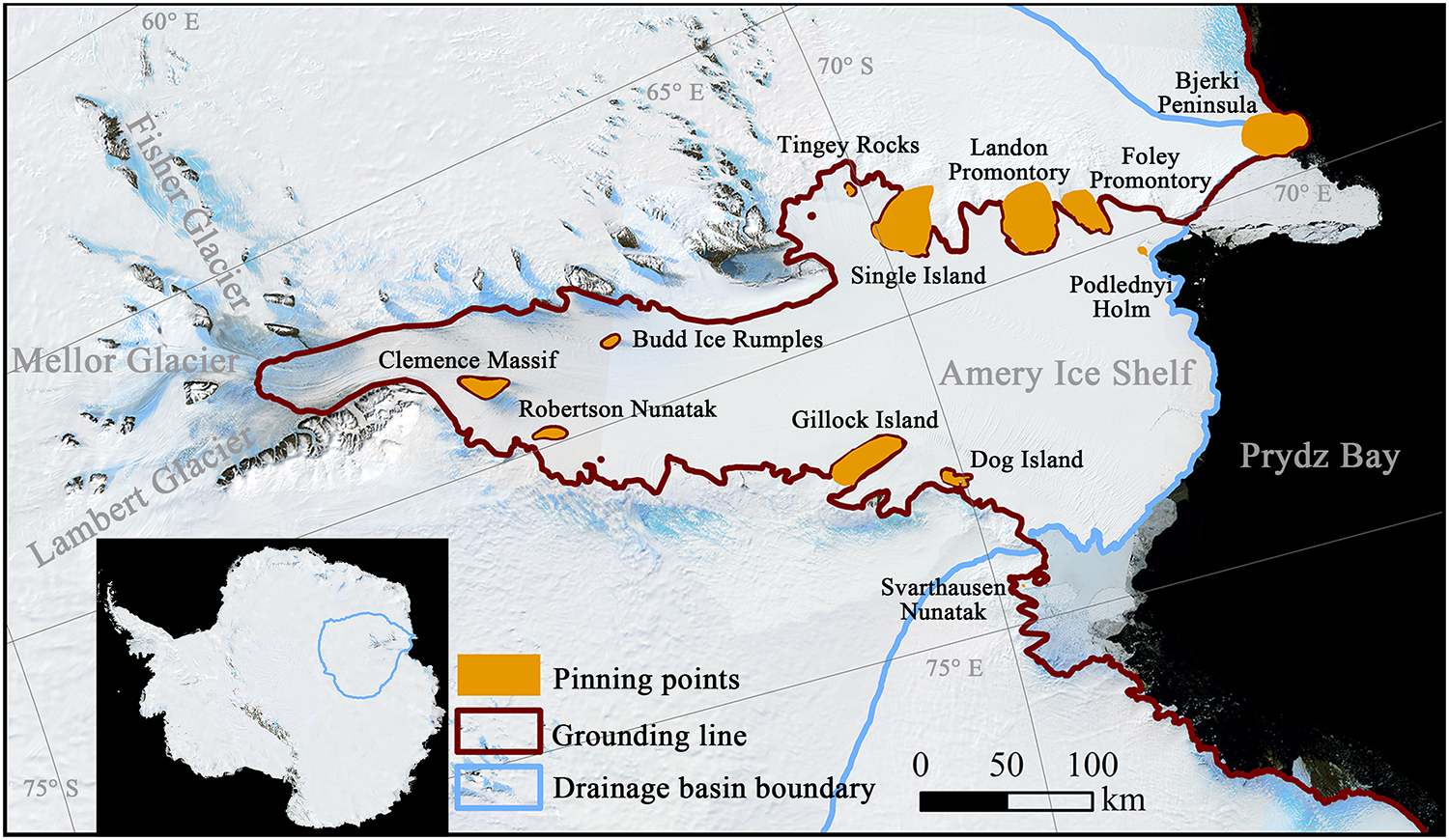
The Lambert–Amery glacial system (LAGS), including the Amery Ice Shelf (AmIS) and its inland drainage (Fig. 1), is one of the largest outlets of the East Antarctic Ice Sheet (EAIS), and its ice-shelf extension provides strong buttressing to inland discharge (Gudmundsson, Reference Gudmundsson2013; Jantre and others, Reference Jantre2024). Although the EAIS is often viewed as comparatively stable, continent-scale syntheses and regional observations reveal marked variability in the mass balance of the EAIS and its fringing East Antarctic ice shelves, underscoring sensitivity to ocean forcing (Shepherd and others, Reference Shepherd2018; Adusumilli and others, Reference Adusumilli, Fricker, Medley, Padman and Siegfried2020; Smith and others, Reference Smith2020). Satellite analyses further document progressive loss or weakening of pinning points (ice rises and rumples) since the 1970s (Miles and Bingham, Reference Miles and Bingham2024), consistent with the hypothesis of an Antarctic ice shelf ‘safety band’, the loss of which would decrease ice shelf buttressing and increase the flux of ice past the grounding line (Fürst and others, Reference Fürst2016). Motivated by these observations, we investigate how ocean-driven changes affect the marine-terminating LAGS and how the persistence or loss of grounded contact at pinning points changes ice discharge under continued ocean warming (Herraiz-Borreguero and others, Reference Herraiz-Borreguero, Coleman, Allison, Rintoul, Craven and Williams2015; Sabu and others, Reference Sabu, Subeesh, Sivakrishnan and Anilkumar2021; Guo and others, Reference Guo, Gao, Shi and Zu2022).
LIMA (Landsat Image Mosaic of Antarctica; Bindschadler and others, Reference Bindschadler2008) mosaic of the Lambert–Amery glacial system (LAGS) and its tributary glaciers (open ocean in black). The grounding line is shown in red (MEaSUREs Antarctic Grounding Line, Version 2; Mouginot and others, Reference Mouginot, Scheuchl and Rignot2017), and the LAGS drainage-basin boundary (coincident with the model domain) is shown in blue (Zwally and others, Reference Zwally, Giovinetto, Beckley and Saba2012). Yellow symbols denote the major named sub-ice-shelf pinning points from the inventory of Matsuoka and others (Reference Matsuoka2015). For clarity, smaller unnamed pinning features are not shown individually in this overview figure; however, the APPs perturbation is applied to all pinning-point polygons within the LAGS basin. Map projection: WGS84 Antarctic Polar Stereographic (EPSG:3031).

Figure 1 Long description
The map depicts the Lambert–Amery glacial system in Antarctica, highlighting key features. The grounding line is marked in red, indicating where the glacier transitions from grounded ice to floating ice. The drainage basin boundary is shown in blue, outlining the area contributing to the glacier's flow. Yellow symbols denote major named sub-ice-shelf pinning points, which are critical for stabilizing the ice shelf. Notable locations include Clemence Massif, Robertson Nunatak and Dog Island. The inset map provides a broader view of Antarctica, with the specific region highlighted. The map includes a scale bar indicating distances in kilometers and a legend explaining the symbols used for pinning points, grounding line and drainage basin boundary.
Recent observations indicate increasing access of relatively warm modified Circumpolar Deep Water (mCDW) to East Antarctic continental shelves and ice-shelf cavities, including the Prydz Bay–Amery sector, with the potential to increase basal melt and promote thinning (Rintoul and others, Reference Rintoul2016; Silvano and others, Reference Silvano2018; Jordan and others, Reference Jordan, Miles, Gudmundsson, Jamieson, Jenkins and Stokes2023). Modeling and process studies highlight efficient on-shelf heat pathways and topographic controls that channel heat toward ice-shelf fronts and grounding zones, with implications for multi-decadal mass loss if intrusions persist (Hirano and others, Reference Hirano2023; Gao and others, Reference Gao2024). Ocean-forced basal melting is now recognized as a dominant driver of Antarctic ice-shelf thinning, with the potential to alter grounding-line position and sea-level contribution (Smith and others, Reference Smith2020).
Ice-shelf geometry shapes how ocean forcing is translated into the spatial pattern and magnitude of basal melt. Basal channels and basal roughness regulate sub-ice circulation and the spatial pattern of basal melt (Cheng and others, Reference Cheng, Jenkins, Holland, Wang, Dong and Liu2024). High-resolution mapping reveals deep troughs and stabilizing ridges beneath Antarctic shelves that influence grounding-zone stability and the emergence of pinning (Morlighem and others, Reference Morlighem2020). These geometric controls make AmIS sensitive to changes that reduce contact at pinning points and weaken buttressing. Buttressing modifies the flux–thickness relationship in a non-monotonic way (Gudmundsson, Reference Gudmundsson2013), and pinning supplies the back-stress that sustains that buttressing. Because buttressing is spatially nonlocal, its magnitude depends not only on how strong each contact is but also on where contacts occur relative to flow and shear margins (Still and others, Reference Still, Campbell and Hulbe2019; Still and Hulbe, Reference Still and Hulbe2021). Consequently, the spatial arrangement of pinning points and the persistence of grounded contact can be as important as the strength of individual contacts.
At the same time, projecting melt at tractable computational cost typically relies on simplified parameterizations of sub-ice-shelf ocean forcing. A further motivation is comparability across Earth system models: parameterizations allow ocean boundary conditions from many CMIP/ISMIP6 AOGCM members to be applied consistently to the same ice-sheet model, providing a controlled way to quantify uncertainty arising from Southern Ocean climate representation. In ISMIP6, basal melt rates are commonly prescribed using quadratic thermal-forcing formulations in a standardized framework (Jourdain and others, Reference Jourdain2020; Nowicki and others, Reference Nowicki2020; Seroussi and others, Reference Seroussi2020). Box-type models such as the Potsdam Ice-shelf Cavity model (PICO) offer an alternative efficient representation of cavity overturning and the translation of basin-scale thermohaline boundary forcing (temperature and salinity) into sub-shelf melt (Reese and others, Reference Reese, Albrecht, Mengel, Asay-Davis and Winkelmann2018), and have been adopted in some ISMIP6 ‘open’ configurations (Seroussi and others, Reference Seroussi2020). Model evaluations indicate that performance is sensitive to unresolved basal geometry. Approaches that account for cavity topography or explicitly represent plumes can substantially alter predicted melt patterns and inferred stability (Lazeroms and others, Reference Lazeroms, Jenkins, Gudmundsson and van de Wal2018; Burgard and others, Reference Burgard, Jourdain, Reese, Favier, Jenkins and Mathiot2022). Together, these uncertainties motivate targeted tests of how loss of grounded contact at AmIS pinning points and unresolved cavity geometry affect buttressing, basal-melt patterns and the sea-level response to ocean forcing.
We quantify how pinning points control basin-scale buttressing and the sea-level contribution of LAGS. We couple Úa to PICO and simulate 2020–2100 under ten SSP5-8.5/RCP8.5 forcings, plus two runs with identical surface mass balance (SMB) and static versus time-evolving basin-mean ocean forcing to isolate ocean effects. To probe the effect of pinning-point/contact geometry, we run a basin-wide ‘all pinning points’ (APPs) case and ten single-point cases. In the APPs case, bed-lowering perturbations are applied to all pinning-point polygons. In each single-point case, the perturbation is applied only to the polygon of one selected pinning point, while all other pinning points are left unmodified, thereby isolating the incremental buttressing contribution of that individual contact. We do not assess how basal melt responds to alternative representations of ice-shelf basal morphology (e.g., channels or roughness). We report the 2100 sea-level contribution, quantify the effect of time-evolving ocean forcing and test how weakening grounded contact at pinning points changes the LAGS response.
Data and methods
Datasets
We use BedMachine Antarctica v3 for bed topography, ice thickness and surface elevation (Morlighem and others, Reference Morlighem2020) (NSIDC-0756), which are interpolated onto the computational mesh (Supplementary Fig. S6). The LAGS drainage-basin mask is taken from the NASA GSFC Cryospheric Sciences Laboratory Antarctic drainage systems (Zwally and others, Reference Zwally, Giovinetto, Beckley and Saba2012).
Large-scale climate forcing is drawn from the ISMIP6 21st Century Forcing Datasets (Nowicki and others, Reference Nowicki, Simon and Team2021), using one simulation each from ten coupled atmosphere–ocean global climate models (AOGCMs) under SSP5-8.5 or earlier-generation RCP8.5 high-emissions scenarios (Jourdain and others, Reference Jourdain2020; Nowicki and others, Reference Nowicki2020). Atmospheric forcing is constructed from the ISMIP6 SMB fields. For each AOGCM member, we add the annual SMB anomaly, defined relative to that member’s 1995–2014 climatology, to the corresponding AOGCM-specific 1995–2014 SMB climatology provided in the forcing dataset. The resulting SMB field is applied as piecewise constant within each year. Thus, the applied SMB forcing retains member-specific differences in both the reference-period SMB climatology and the transient SMB anomaly; this should be considered when interpreting the inter-member spread in the atmospheric forcing contribution.
Basal melt parameterization (PICO)
Sub-ice-shelf basal melt beneath floating ice is computed using the PICO parameterization (Reese and others, Reference Reese, Albrecht, Mengel, Asay-Davis and Winkelmann2018), forced by ISMIP6 ocean temperature and salinity fields in a manner consistent with the ISMIP6 Antarctica experimental framework (including ‘open’ melt configurations) (Seroussi and others, Reference Seroussi2020). Where implementation choices exist in PICO (e.g., the delineation of connected floating regions and the criterion used to identify floating nodes), we use the watershed-based shelf delineation and the GLthreshold floating criterion (Supplementary Table S1); otherwise, we follow the Amery-specific setup described by Reese and others (Reference Reese, Albrecht, Mengel, Asay-Davis and Winkelmann2018). Two parameters are tuned within standard ranges to improve the sub-ice-shelf basal-melt magnitude and spatial pattern across members: the effective turbulent temperature exchange velocity  $\gamma_T^\ast = 1.5\times 10^{-4}~\mathrm{m~s}^{-1}$ and the maximum number of overturning boxes $n_{\max} = 10$. For PICO boundary conditions, we construct a yearly time series by averaging ISMIP6 temperature $T$ and salinity $S$ within a 50 km ocean strip seaward of the Amery front for each basin, which provides a representative shelf-water signal while suppressing local-scale noise. The resulting melt fields are evaluated against the satellite-constrained basal-melt product of Adusumilli and others (Reference Adusumilli, Fricker, Medley, Padman and Siegfried2020) in the following section.
Model setup and initialization
Ice flow is simulated with the SSA-based Úa model coupled to PICO (Reese and others, Reference Reese, Albrecht, Mengel, Asay-Davis and Winkelmann2018; Gudmundsson, Reference Gudmundsson2020). The baseline mesh follows the ‘Amery Ice Shelf grid-sensitivity case’ of Wang and others (Reference Wang, Li, Cheng, Zhao, Zheng and Liang2024) and is refined to 1 km within a  $\pm 30$ km buffer of all grounding-line segments across the domain to resolve grounding-line migration, stress gradients and pinning contacts (Supplementary Fig. S6). The pinning points perturbed here lie predominantly within the main grounding-line-adjacent belt (Supplementary Fig. S11) and are therefore covered by this refinement. Glen’s flow law uses exponent $n = 3$. The depth-averaged rate factor $A$ and the basal slipperiness $C$ are inferred by inverse modeling following Wang and others (Reference Wang, Li, Cheng, Zhao, Zheng and Liang2024) and then held fixed in all forward runs.
To suppress artifacts arising from observational noise and resolution mismatch, we first perform a short relaxation. Starting from the inversion-derived present-day state, we time-integrate the coupled Úa–PICO model for 20 years with  $\Delta t = 0.5~\mathrm{yr}$ under a time-invariant 2020 CCSM4 climate snapshot. During this relaxation, both the atmospheric forcing (SMB) and the PICO ocean boundary conditions ( $T$–
$T$– $S$) are taken from CCSM4-rcp85 at year 2020. The end state of this relaxation is hereafter referred to as the common 2020-relaxed state and is used as the initial condition for all projection experiments. CCSM4 is used only to provide a single internally consistent 2020 forcing snapshot for the relaxation.
From this common 2020-relaxed state, the subsequent ISMIP6 forcings are applied directly, i.e., not as anomalies relative to the CCSM4 relaxation forcing. We then run two types of AOGCM-forced experiments. First, the transient experiments use each AOGCM member’s time-evolving SMB and ocean  $T$–
$T$– $S$ forcing for 2020–2100. Second, to diagnose the adjustment caused by switching from the common 2020-relaxed state to a different member’s 2020 forcing, we run member-specific 2020-constant simulations. In these simulations, the model starts from the same common 2020-relaxed state, but each AOGCM member’s 2020 SMB field and PICO ocean boundary conditions are held constant through 2100. These 2020-constant simulations therefore quantify the fixed-forcing adjustment that would occur without post-2020 forcing evolution (Supplementary Fig. S8).
For the sea-level contribution emphasized here, each transient experiment is paired with its corresponding member-specific 2020-constant simulation. These pairs provide the basis for the transient-minus-2020-constant diagnostic used below to isolate the response to post-2020 forcing evolution (Supplementary Fig. S9).
Experiments and pinning perturbations
We perform twelve projections for 2020–2100: ten experiments forced by distinct ISMIP6 AOGCMs (each using that model’s time-evolving SMB and ocean  $T$,
$T$,  $S$ fields), and two control runs. The AOGCM members are listed and shown with consistent styling in Supplementary Figs. S1–S3. Ctrl-Static prescribes time-invariant 2020 ensemble-mean forcing: SMB is the ten-model ensemble-mean 2020 climatology, and basal mass balance (BMB) is computed with PICO forced by the ensemble-mean 2020 basin $T_0$, $S_0$. Ctrl-OceanAvg keeps SMB identical to Ctrl-Static but drives PICO with the time-evolving ensemble-mean basin $T(t)$, $S(t)$ for 2020–2100, so only BMB varies in time. All experiments share the same mesh, numerical settings and boundary conditions, and all start from the common 2020-relaxed state.
To probe buttressing sensitivity, we apply targeted topographic perturbations strictly within the pinning polygons of Matsuoka and others (Reference Matsuoka2015). The magnitude (500 m bed lowering) follows Still and Hulbe (Reference Still and Hulbe2021); here it is used as a deliberate de-buttressing test rather than a realistic target. We consider (i) a basin-wide ‘all pinning points’ (APPs) case, repeated under every forcing member (the ten AOGCM forcings and both controls), and (ii) ten single-point cases targeting the ten largest pinning points beneath AmIS, run under Ctrl-Static to isolate forcing effects. In each single-point case, the bed is lowered within the polygon of one selected pinning point only, while the rest of the bed, including all other pinning points, is kept unchanged. Thus, these experiments isolate the buttressing contribution of removing contact at one pinning point at a time, rather than retaining only one active pinning point. Of twelve candidates initially identified, BedMachine v3 indicates that Podlednyj Holm is no longer grounded and Svarthausen Nunatak lies outside the LAGS drainage, leaving ten pinning points for the single-point tests. The remaining smaller and/or unnamed pinning polygons are included in APPs but not treated individually; together, they account for only 108.84 km $^2$ out of 4300.80 km $^2$ of the total pinning area within LAGS.
Results
Basal melt: observed pattern vs. PICO ensemble
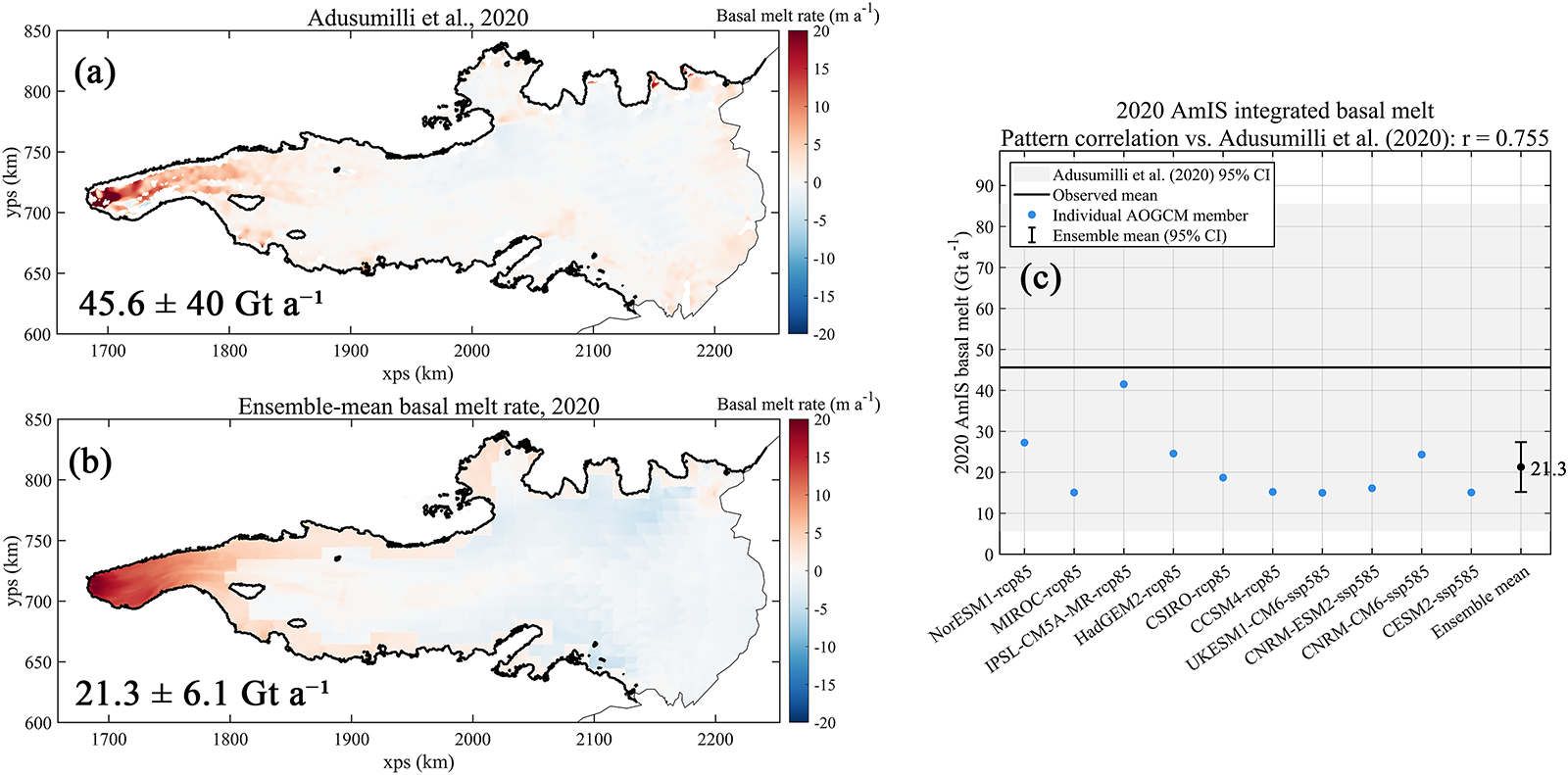
The 2020 basal melt pattern from Adusumilli and others (Reference Adusumilli, Fricker, Medley, Padman and Siegfried2020) (Fig. 2a) shows intense melt concentrated near the southern inlet and at a few shelf–topography interaction sites, with broad areas of weak melt or refreezing elsewhere. The PICO ensemble mean for the ten climate forcings (Fig. 2b) reproduces the large-scale structure of the Adusumilli map, including the high-melt tongue at the western front and the low-melt interior, while smoothing small-scale extremes as expected from the box parameterization.
2020 basal melt of AmIS. (a) Observation-based basal melt rate from Adusumilli and others (Reference Adusumilli, Fricker, Medley, Padman and Siegfried2020) (m a $^{-1}$), with the domain-integrated total and its 95% confidence interval (CI) indicated. (b) PICO 10-member ensemble-mean basal melt rate (m a $^{-1}$), with the corresponding domain-integrated total indicated. (c) Domain-integrated basal melt (Gt a $^{-1}$): the gray band shows the observation-based 95% CI from Adusumilli and others (Reference Adusumilli, Fricker, Medley, Padman and Siegfried2020), and the horizontal black line marks the corresponding observation-based mean. Colored symbols show the integrated melt for individual AOGCM members (single values, no uncertainty range shown); the rightmost black symbol shows the ensemble mean, with error bars indicating the 95% CI of the mean. Inset: pattern correlation between the PICO ensemble mean and the Adusumilli field, $r=0.755$.

Figure 2 Long description
The figure consists of three panels comparing basal melt rates and integrated melt for the Amundsen Sea Ice Shelf (AmIS) in 2020. Panel (a) shows an observation-based basal melt rate map from Adusumilli and others, with values in m a superscript minus 1. The map highlights intense melt near the southern inlet and shelf-topography interaction sites, with a total melt of 45.6 plus or minus 40 Gt a superscript minus 1. Panel (b) displays the PICO 10-member ensemble-mean basal melt rate, also in m a superscript minus 1, showing a similar pattern but with smoother extremes and a total melt of 21.3 plus or minus 6.1 Gt a superscript minus 1. Panel (c) is a scatter plot titled '2020 AmIS integrated basal melt: Pattern correlation vs. Adusumilli et al. (2020), r equals 0.755'. The x-axis lists different AOGCM members and the y-axis represents the integrated basal melt in Gt a superscript minus 1. The plot includes individual member values, a horizontal line indicating the observation-based mean and a shaded band showing the 95 percent confidence interval. The ensemble mean is marked with an error bar, showing a lower melt compared to the observation-based data. This figure illustrates the spatial and quantitative differences between observed and modeled basal melt rates.
Integrated over AmIS, the observation-based estimate is  $45.6 \pm 40~\mathrm{Gt~a^{-1}}$ (95% confidence interval (CI)). The PICO ensemble mean yields $21.3 \pm 6.1~\mathrm{Gt~a^{-1}}$ (95% CI). Thus, the ensemble mean lies within the observation-based 95% confidence interval, but even the upper end of the ensemble remains below the Adusumilli central estimate. A quantitative comparison of spatial structure (Fig. 2c) gives a pattern correlation $r = 0.755$ between the PICO ensemble mean and the Adusumilli field, indicating that the parameterized melt captures most of the observed spatial variability.
The temporal evolution of AmIS-integrated basal melt is summarized in Supplementary Fig. S1 (with the corresponding heat map in Supplementary Fig. S1b). Across most forcings, basal melt increases from  $\sim\!20~\mathrm{Gt~a^{-1}}$ in 2020 to $\sim\!100$– $300~\mathrm{Gt~a^{-1}}$ by 2100. As an upper-end geometric context, Supplementary Fig. S7 shows the 2020–2100 evolution of ice and bed elevation along the flowline (the blue line in Supplementary Fig. S6) for CNRM-ESM2–SSP5-8.5, which produces the strongest sub-shelf melt in our ensemble; even in this case, thinning by 2100 remains limited to $\sim\!600$ m within $\sim\!100$ km downstream of the grounding line. Ctrl-Static remains nearly constant at $\sim\!20~\mathrm{Gt~a^{-1}}$ by design, whereas Ctrl-OceanAvg rises gradually to $\sim\!160~\mathrm{Gt~a^{-1}}$. The ensemble median increases monotonically, and the inter-model spread diverges from $\sim\!15$– $27~\mathrm{Gt~a^{-1}}$ in 2020 to roughly $\sim\!100$– $300~\mathrm{Gt~a^{-1}}$ by 2100. As expected for our PICO set-up with basin-mean ocean boundary conditions, bed-perturbed and unperturbed pairs exhibit nearly indistinguishable shelf-integrated basal melt, so the prescribed bed perturbations do not materially alter the melt forcing over 2020–2100. We therefore interpret the resulting changes in volume above flotation ( $\Delta\mathrm{VAF}$) primarily as a dynamical buttressing response to contact loss.
System-scale evolution and the effect of simultaneous pinning loss
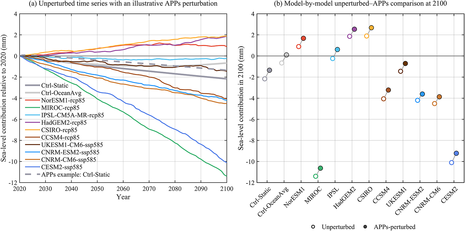
Across the twelve applied forcings, LAGS shows a predominantly negative or near-zero sea-level contribution over 2020–2100 (Fig. 3), equivalent to predominantly positive  $\Delta\mathrm{VAF}$. By 2100, $\Delta\mathrm{VAF}$ spans roughly $-7\times 10^{2}$ to $4\times 10^{3}~\mathrm{Gt}$ (from CSIRO-rcp85 to MIROC-rcp85), corresponding to an SLR contribution of about $-11.4$ to $1.9~\mathrm{mm}$ (Fig. 3b; Supplementary Fig. S3a). Most forcings (7/12) yield negative SLR contributions by 2100, indicating net VAF gain; the remaining forcings are near-zero or slightly positive, including NorESM1-rcp85, HadGEM2-rcp85 and CSIRO-rcp85. These trajectories are therefore interpreted as absolute outcomes under the applied forcing protocol, rather than as drift-corrected estimates of the response to post-2020 forcing evolution alone.
Sea-level contribution of LAGS relative to 2020 in the control and transient experiments initialized from the common 2020-relaxed state. (a) Unperturbed time series for Ctrl-Static, Ctrl-OceanAvg and the ten AOGCM transient-forcing runs. The dashed curve shows an illustrative APPs perturbation under Ctrl-Static, in which all pinning points are weakened. (b) Sea-level contribution in 2100 for each forcing. Open circles show unperturbed simulations, filled circles show the corresponding APPs perturbation experiments and gray lines connect each perturbed–unperturbed pair. Ctrl-Static uses time-invariant ensemble-mean 2020 SMB and ocean forcing for PICO, whereas Ctrl-OceanAvg uses the same SMB but time-evolving ensemble-mean basin  $T$ and $S$. The AOGCM transient trajectories are absolute outcomes relative to the common 2020-relaxed state. Supplementary Fig. S8 quantifies the fixed-forcing adjustment caused by switching from this state to member-specific 2020 forcing, whereas Supplementary Fig. S9 isolates the response to post-2020 forcing evolution using transient-minus-2020-constant differences.

Figure 3 Long description
The figure contains two panels showing the sea-level contribution of the Lambert–Amery glacial system relative to 2020. Panel a is a time-series line plot from 2020 to 2100. The horizontal axis is labelled Year, and the vertical axis is labelled Sea-level contribution in millimetres, with values spanning approximately −12 to +4 mm. All curves start close to zero in 2020 and diverge over time. The solid curves show the unperturbed simulations for Ctrl-Static, Ctrl-OceanAvg and the ten AOGCM transient-forcing experiments. By 2100, some trajectories remain close to zero or become slightly positive, whereas others become increasingly negative, reaching about −11 mm in the most negative case. A dashed curve shows an illustrative APPs perturbation under Ctrl-Static, in which all pinning points are weakened. Panel b is a paired scatter plot showing the 2100 sea-level contribution for each forcing. The horizontal axis lists Ctrl-Static, Ctrl-OceanAvg and the ten AOGCM transient-forcing experiments. The vertical axis again shows sea-level contribution in millimetres, spanning approximately −12 to +4 mm. For each forcing, an open circle represents the unperturbed simulation and a filled circle represents the corresponding APPs perturbation experiment. Grey line segments connect each perturbed–unperturbed pair. The filled circles are generally slightly higher than the corresponding open circles, indicating that weakening all pinning points increases the sea-level contribution relative to the unperturbed case.
To assess the effect of switching from the common 2020-relaxed state to each member’s 2020 forcing, we use the member-specific 2020-constant simulations. For a diagnostic variable  $X$ (e.g., $\Delta\mathrm{VAF}$ or SLR contribution), the member-specific fixed-forcing adjustment is quantified as
 \begin{equation}
X_i^{\mathrm{2020const}}(t)-X_{\mathrm{CCSM4}}^{\mathrm{2020const}}(t),
\end{equation}
\begin{equation}
X_i^{\mathrm{2020const}}(t)-X_{\mathrm{CCSM4}}^{\mathrm{2020const}}(t),
\end{equation}where  $X_i^{\mathrm{2020const}}$ is the 2020-constant simulation for AOGCM member $i$ and $X_{\mathrm{CCSM4}}^{\mathrm{2020const}}$ is the CCSM4 2020-constant continuation. Relative to the CCSM4 2020-constant continuation, the member-specific 2020-constant simulations span $-2.34\times10^{3}$ to $3.95\times10^{3}~\mathrm{Gt}$ in $\Delta\mathrm{VAF}$ by 2100, corresponding to an SLR range of $-10.93$ to $+6.47~\mathrm{mm}$ (Supplementary Fig. S8). This range is comparable to the spread of the absolute transient AOGCM ensemble, indicating that the trajectories in Fig. 3 include a substantial fixed-forcing adjustment from the common 2020-relaxed state.
To further isolate the response to post-2020 forcing evolution, we compare each transient experiment with its corresponding member-specific 2020-constant simulation:
 \begin{equation}
X_i^{\mathrm{transient}}(t)-X_i^{\mathrm{2020const}}(t).
\end{equation}
\begin{equation}
X_i^{\mathrm{transient}}(t)-X_i^{\mathrm{2020const}}(t).
\end{equation} This transient-minus-2020-constant diagnostic removes each member’s own fixed-forcing adjustment and measures the additional response to time-evolving forcing after 2020 (Supplementary Fig. S9). By 2100, this response spans  $-3.84$ to $+4.66~\mathrm{mm}$ SLR across the ten AOGCM members. Thus, post-2020 forcing evolution produces a detectable additional response, while the absolute AOGCM-forced trajectories also retain a substantial member-specific fixed-forcing adjustment from the common 2020-relaxed state. The absolute AOGCM-forced trajectories in Fig. 3 therefore represent combined outcomes of member-specific fixed-forcing adjustment and response to time-evolving climate forcing.
Notably, MIROC-rcp85 and CSIRO-rcp85 have similar AmIS-integrated basal-melt evolution (Supplementary Fig. S1) but opposite-sign 2100 sea-level contributions (Supplementary Fig. S3a), consistent with their contrasting domain-integrated SMB (Supplementary Fig. S2); this underscores that melt-driven changes should be interpreted together with the overall SMB evolution.
The two control runs illustrate the sensitivity to ocean forcing under two contrasting representations, rather than providing a strict upper and lower bound on its contribution. Ctrl-Static (dark-gray solid) shows an almost linear decrease in SLR, reaching  $-2.17$ mm by 2100. Ctrl-OceanAvg (light-gray solid), with PICO forced by time-evolving basin-mean $T$ and $S$, yields a less negative SLR trajectory, reaching $-0.67$ mm by 2100: ocean warming enhances shelf basal melt, weakens buttressing and increases grounded-ice discharge to the shelf, thereby increasing SLR relative to Ctrl-Static. Because SMB is identical in both control runs and the SMB-associated VAF gain remains larger than the ocean-driven dynamic loss, SLR remains negative in Ctrl-OceanAvg. This suggests that, in this SMB-identical control comparison, ocean-driven dynamic loss is insufficient to offset the SMB-associated VAF gain by 2100.
Bed-perturbed experiments, in which all pinning points are weakened simultaneously under the same climate as their corresponding unperturbed runs, shift trajectories toward higher SLR. Comparing the unperturbed and APPs heat maps (Supplementary Fig. S3a,b) shows that bed-perturbed minus unperturbed SLR at 2100 is about  $+0.6$ to $+0.9~\mathrm{mm}$ (mean $0.82~\mathrm{mm}$), indicating a quasi-constant buttressing penalty that is largely independent of the forcing. Notably, the integrated basal-melt rates of perturbed–unperturbed pairs are nearly indistinguishable (Supplementary Fig. S1), implying that the SLR sensitivity mainly reflects reduced buttressing rather than cavity-melt changes, which motivates the single-pinning-point analysis in the following section.
Single-pinning-point contributions to SLR and response timing
All single-pinning-point experiments are run under Ctrl-Static. We define
 \begin{equation}
\Delta\mathrm{SLR}_i(t)
= \mathrm{SLR}_{\mathrm{perturbed},i}(t)
- \mathrm{SLR}_{\textit{Ctrl-Static}}(t),
\end{equation}
\begin{equation}
\Delta\mathrm{SLR}_i(t)
= \mathrm{SLR}_{\mathrm{perturbed},i}(t)
- \mathrm{SLR}_{\textit{Ctrl-Static}}(t),
\end{equation}where  $\Delta\mathrm{SLR}_i(t)$ is the sea-level contribution of perturbation $i$ relative to the Ctrl-Static simulation. For clarity, we denote the 2100 sea-level response of perturbation $i$ as $y_i=\Delta\mathrm{SLR}_i(2100)$, and the corresponding magnitude of the 2100 grounding-area change as $x_i$. Here, $x_i$ is defined as the magnitude of the domain-integrated grounded-area difference between the perturbed and control simulations,
 \begin{equation}
x_i = \left|A_{\mathrm{perturbed},i}(2100)-A_{\textit{Ctrl-Static}}(2100)\right|,
\end{equation}
\begin{equation}
x_i = \left|A_{\mathrm{perturbed},i}(2100)-A_{\textit{Ctrl-Static}}(2100)\right|,
\end{equation}reported in km $^2$. For most perturbations this corresponds to grounding-area loss; for re-grounding cases such as Clemence Massif, it should be interpreted as the magnitude of the grounding-area change. This domain-integrated metric captures the net grounding response attributable to weakening pinning point $i$, including any grounding-line migration that is dynamically triggered by the local reduction in buttressing. The APPs marker (Ctrl-Static) denotes the basin-wide case in which all pinning points are weakened simultaneously.
To quantify local re-grounding at each perturbed pinning point, we track grounded-area changes within the fixed perturbation polygon used to impose the bed perturbation. We define the late-century re-grounding area fraction  $F_{\mathrm{ReGA}}$ as the 2080–2100 mean of the grounded fraction within that polygon in the perturbed simulation, i.e.
 \begin{equation}
F_{\mathrm{ReGA}}=\overline{A_{\mathrm{perturbed}}/A_{\mathrm{poly}}}^{\,2080\text{--}2100},
\end{equation}
\begin{equation}
F_{\mathrm{ReGA}}=\overline{A_{\mathrm{perturbed}}/A_{\mathrm{poly}}}^{\,2080\text{--}2100},
\end{equation}where  $A_{\mathrm{poly}}$ is the area of the perturbation polygon. Time series of grounded area within each perturbation polygon, used to compute $F_{\mathrm{ReGA}}$, are shown in Supplementary Fig. S5. To quantify response timing, we further define an emergence time $t_{50\%}$ for each experiment as the first year when the 3 year running mean of $\Delta\mathrm{SLR}_i(t)$ reaches 50% of its own late-century (2080–2100) mean. This metric captures how rapidly the sea-level signal becomes established while remaining robust to early transient variability.
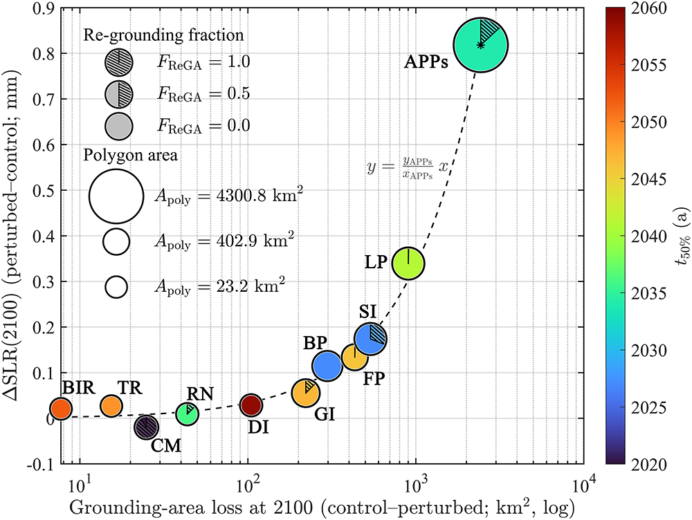
At 2100 the single-point results cluster around the APPs proportionality  $y_i = \beta x_i$ (Fig. 4; $x$-axis logarithmic for visualization only), where $\beta = y_{\mathrm{APPs}}/x_{\mathrm{APPs}}$ and equals $3.36\times 10^{-4}~\mathrm{mm~km^{-2}}$ in this configuration. No regression was fitted; the dashed line is defined by the APPs point. Absolute departures from this proportionality are small ( $\mathrm{MAD}(\mathrm{res}) = 0.017~\mathrm{mm}$; $\mathrm{RMSE}(\mathrm{res}) = 0.019~\mathrm{mm}$). Small losses ( $\lesssim 100~\mathrm{km^2}$) yield near-zero response, consistent with the mesh-limited effective resolution of grounding transitions or with rapid local re-grounding that offsets the initial loss, and the removed contact area is intrinsically too small to appreciably alter shelf-scale buttressing.
Sea-level contribution versus grounding-area loss at 2100 for individual pinning points in LAGS. The  $x$-axis shows $x_i$, the magnitude of the 2100 domain-integrated grounded-area difference between the perturbed and Ctrl-Static simulations (km $^2$; logarithmic scale). The $y$-axis shows the 2100 sea-level contribution, $y_i=\Delta\mathrm{SLR}_i(2100)$, defined as the perturbed-minus-control sea-level contribution difference (mm). Circle area represents the perturbation-polygon area, $A_{\mathrm{poly}}$. The shaded fraction within each circle shows the late-century re-grounding fraction, $F_{\mathrm{ReGA}}$, defined as the mean grounded fraction within the perturbation polygon over 2080–2100. Color shows $t_{50\%}$, the first year when the 3 year running mean of $\Delta\mathrm{SLR}_i(t)$ reaches 50% of its own 2080–2100 mean. The APPs circle denotes the basin-wide perturbation under Ctrl-Static, in which the bed is lowered within all pinning-point polygons. The dashed reference line shows $y =(y_{\mathrm{APPs}}/x_{\mathrm{APPs}})\,x$. The slope $y_{\mathrm{APPs}}/x_{\mathrm{APPs}}$ can be interpreted as the average LAGS shelf-scale buttressing efficiency associated with pinning-contact loss.

Figure 4 Long description
Figure 4 is a scatter plot showing sea-level contribution versus grounding-area loss at 2100 for individual pinning points in the Lambert–Amery glacial system. The horizontal axis shows the magnitude of the 2100 domain-integrated grounded-area difference between the perturbed and Ctrl-Static simulations, (x_i), in km(^2), plotted on a logarithmic scale. The vertical axis shows the 2100 sea-level contribution, (y_i=\Delta \mathrm{SLR}_i(2100)), in millimetres, defined as the perturbed-minus-control sea-level contribution difference. The y-axis spans approximately (-0.1) to (0.9) mm. Each circle represents one perturbation experiment. Circle area indicates the perturbation-polygon area, (A_{\mathrm{poly}}). The size legend shows three example polygon areas: (23.2) km(^2), (402.9) km(^2), and (4300.8) km(^2). The shaded fraction within each circle indicates the late-century re-grounding fraction, (F_{\mathrm{ReGA}}), defined as the mean grounded fraction within the perturbation polygon over 2080–2100. The re-grounding legend shows three example values: (F_{\mathrm{ReGA}}=0.0), (0.5), and (1.0). Circle colour shows (t_{50%}), the first year when the 3-year running mean of (\Delta \mathrm{SLR}_i(t)) reaches 50% of its own 2080–2100 mean; the colour scale ranges from 2020 to 2060. The APPs circle denotes the basin-wide perturbation under Ctrl-Static, in which the bed is lowered within all pinning-point polygons. A dashed reference line shows (y=(y_{\mathrm{APPs}}/x_{\mathrm{APPs}}),x). The slope (y_{\mathrm{APPs}}/x_{\mathrm{APPs}}) represents the average LAGS shelf-scale buttressing efficiency associated with pinning-contact loss.
Landon Promontory (LP) and Single Island (SI) are the largest contributors, with  $\Delta\mathrm{SLR}_{2100}$ of $0.34~\mathrm{mm}$ and $0.17~\mathrm{mm}$, respectively. Foley Promontory (FP) and Bjerki Peninsula (BP) follow ( $\sim\!0.11$– $0.13~\mathrm{mm}$), while Gillock Island (GI) is smaller ( $\sim\!0.06~\mathrm{mm}$). Several features are weak or near-neutral, for example, Robertson Nunatak (RN) ( $\sim\!0.01~\mathrm{mm}$), Dog Island (DI) ( $\sim\!0.03~\mathrm{mm}$) and Tingey Rocks (TR) ( $\sim\!0.03~\mathrm{mm}$). Clemence Massif (CM) yields a small negative response ( $\sim\!-0.02~\mathrm{mm}$). The 500 m lowering produces rapid re-grounding over $\sim\!40\%$ of the polygon. In the baseline (unperturbed Ctrl-Static), CM is a local bed high with little or no shelf-ice cover; once the nunatak is lowered, shelf ice quickly overruns and re-grounds there, so most of the area is grounded by late century, increasing back-stress and slightly reducing discharge (Supplementary Fig. S12).
High-impact points such as LP, FP and BP show low late-century re-grounding fractions ( $F_{\mathrm{ReGA}}$), implying limited local recovery and therefore a sustained sea-level response. By contrast, CM shows strong re-grounding ( $F_{\mathrm{ReGA}} = 0.90$) and a small negative $\Delta\mathrm{SLR}(2100)$, consistent with stabilizing new grounding. RN also has a small overall impact despite low re-grounding, indicating weak leverage on shelf-scale buttressing. GI lies only slightly below the APPs reference slope in Fig. 4; together with its low re-grounding fraction ( $F_{\mathrm{ReGA}} = 0.12$) and small 2100 response ( $\Delta\mathrm{SLR}(2100) = 0.06~\mathrm{mm}$), this suggests a buttressing efficiency that is slightly lower than the APPs average. Additional diagnostics (Supplementary Fig. S10) are broadly consistent with relatively weak local stress transmission and partial interior re-grounding, although the departure from the APPs reference slope is small. By comparison, BP and LP lie slightly above the APPs reference slope, indicating somewhat higher-than-average buttressing efficiency. SI provides an illustrative intermediate case: it loses a large grounding area ( $\sim\!537~\mathrm{km^2}$) but shows moderate re-grounding ( $F_{\mathrm{ReGA}} = 0.31$), yielding a modest 2100 contribution ( $\Delta\mathrm{SLR}(2100) = 0.17~\mathrm{mm}$). Its proximity to the APPs reference slope is consistent with quasi-linear scaling of $\Delta\mathrm{SLR}(2100)$ with grounding-area loss, with the muted magnitude explained mainly by partial re-grounding rather than unusually weak buttressing.
The simple sum of the ten single-point contributions at 2100 is  $0.88~\mathrm{mm}$, whereas the APPs response is $0.82~\mathrm{mm}$, a difference of $0.06~\mathrm{mm}$ (about $7\%$). By comparison, the summed grounding-area loss across the ten single-point experiments is $2586.72~\mathrm{km^2}$, close to the APPs value of $2434.04~\mathrm{km^2}$, with a difference of $152.68~\mathrm{km^2}$ (about $6\%$). Although the APPs experiment includes all pinning points within LAGS, whereas the single-point set samples only the ten major named features, the similar fractional differences in sea-level response and grounding-area loss are nevertheless consistent with a near-linear relation between $\Delta\mathrm{SLR}_{2100}$ and grounding-area loss, with only modest departures from perfect additivity among the dominant contacts.
Discussion
Across the ten SSP5-8.5/RCP8.5 forcings, the absolute basin-scale sea-level contribution of LAGS by 2100 remains close to zero under the applied forcing protocol. The two control runs illustrate the ocean role: with SMB held fixed, replacing a static basin-mean temperature–salinity series with a time-evolving one changes 2100 SLR by  $1.50~\mathrm{mm}$, corresponding to $-2.17~\mathrm{mm}$ (Ctrl-Static) versus $-0.67~\mathrm{mm}$ (Ctrl-OceanAvg) by 2100. Ocean forcing therefore matters in our set-up but is not decisive at century scale.
The geometry tests isolate buttressing. When all pinning points are weakened together, the 2100 SLR penalty is  $0.82~\mathrm{mm}$ and is nearly independent of forcing (Fig. 3; Supplementary Fig. S3b). Single-point experiments show that the 2100 $\Delta\mathrm{SLR}$ for a site increases with its grounding-area loss, and the points cluster about a reference proportionality $y_i = \beta x_i$, where $\beta$ is an average shelf-scale buttressing efficiency for AmIS in this configuration with units of mm SLR per km $^2$ grounding-area loss (Fig. 4). The APPs response is $0.06~\mathrm{mm}$ (about 7%) below the linear sum of the ten single-point contributions, indicating a collective response that is close to linear; absolute departures are small (MAD $= 0.017~\mathrm{mm}$; RMSE $= 0.019~\mathrm{mm}$).
Quasi-linear scaling follows from where contacts act and how weakly they interact. Ice-shelf buttressing modifies the flux–thickness relation at the grounding line and depends on the spatial distribution of back-stress (Gudmundsson, Reference Gudmundsson2013). Maps of Antarctic ‘safety bands’ identify the belt adjacent to the grounding line as the region where loss of contact most strongly increases grounded-ice discharge (Fürst and others, Reference Fürst2016). In our AmIS geometry, most pinning points fall within this grounding-line-adjacent belt (Supplementary Fig. S11). This focus on the first  $\sim$20 km downstream of the grounding line is also consistent with independent buttressing diagnostics for AmIS (Wang and others, Reference Wang, Li, Cheng, Zhao, Zheng and Liang2024), which indicate that the dominant share of buttressing is concentrated within this near-grounding-line zone. To first order, if we ignore strong stress overlap among neighboring contacts, substantial re-grounding, threshold-type grounding-line transitions and large melt-pattern reorganizations, the sea-level response scales with total grounding-area loss. This yields the observed near-linear relation $y_i = \beta x_i$. The small shortfall between APPs and the linear sum is consistent with modest interaction among nearby contacts and a slowly varying grounding-line sensitivity within the belt (Gudmundsson, Reference Gudmundsson2013; Fürst and others, Reference Fürst2016). Case studies that weaken individual contacts generally find a first-order, size-controlled response with second-order, site-dependent variations in the impact (e.g., due to along-grounding-line variations in sensitivity and partial stress-overlap among nearby contacts); under similar near-grounding-line settings, this often yields approximately additive behavior (Still and Hulbe, Reference Still and Hulbe2021; Wild and others, Reference Wild, Alley, Muto, Truffer, Scambos and Pettit2022). Our AmIS results are consistent with this picture, with the magnitude of effective contact loss explaining most of the variance and only a few cases deviating from additivity.
Site-to-site differences primarily reflect the magnitude of the buttressing effect. Landon Promontory and Single Island are most influential; Foley Promontory and Bjerki Peninsula follow; Gillock Island is modest. For GI, additional diagnostics (Supplementary Fig. S10) are broadly consistent with relatively weak local stress transmission and partial interior re-grounding ( $F_{\mathrm{ReGA}}=0.12$), which may help explain both its modest overall buttressing effect and why its buttressing efficiency is slightly lower than the APPs reference slope $y_i = \beta x_i$. Clemence Massif is stabilizing because bed-lowering there induces early re-grounding that persists where baseline thickness is near zero (high $F_{\mathrm{ReGA}}$), increasing contact area and back-stress. Two diagnostics account for most of the spread: the late-century re-grounding area fraction $F_{\mathrm{ReGA}}$ (persistence) and the emergence time $t_{50\%}$ (timing). High-impact sites tend to have low $F_{\mathrm{ReGA}}$ and respond early; high $F_{\mathrm{ReGA}}$ damps the response (Fig. 4).
Perturbed–unperturbed pairs have nearly identical shelf-integrated basal melt (Supplementary Figs. S1a and S4a) but different SLR trajectories (Supplementary Fig. S3), indicating that century-scale differences are driven primarily by changes in buttressing rather than by changes in melt forcing. This behavior is expected for the PICO configuration adopted here: melt is computed under prescribed basin-mean ocean boundary conditions in a coarse, box-based framework, so small, localized geometric perturbations at individual pinning points are not anticipated to substantially reorganize the melt pattern or alter the shelf-integrated melt when the ocean forcing is held fixed. Within this scope, the ensemble reproduces the observed large-scale melt structure with good pattern skill (pattern correlation  $r=0.755$), although the integrated magnitude is lower than the observation-based central estimate (Fig. 2; Reese and others Reference Reese, Albrecht, Mengel, Asay-Davis and Winkelmann2018; Adusumilli and others Reference Adusumilli, Fricker, Medley, Padman and Siegfried2020; Jourdain and others Reference Jourdain2020). We note that at finer spatial scales, geometry-aware and plume-based schemes can reshape melt distributions and associated stress transmission (Lazeroms and others, Reference Lazeroms, Jenkins, Gudmundsson and van de Wal2018; Burgard and others, Reference Burgard, Jourdain, Reese, Favier, Jenkins and Mathiot2022), and circulation-resolving ocean models including tides and channelized flows may increase the sensitivity of integrated melt to contact loss. Accordingly, our experiments should be interpreted as isolating the dynamical response to pinning-point weakening under a controlled melt forcing, with melt–geometry feedbacks beyond the representation of PICO deferred to future work.
Because  $\Delta\mathrm{SLR}$ scales approximately with grounding-area loss, three metrics are potentially useful: (i) grounding-area loss at high-impact sites, (ii) $F_{\mathrm{ReGA}}$ as a persistence indicator and (iii) early evolution of $t_{50\%}$ as a timing indicator. Operational mapping of contact extent and thickness near Landon Promontory, Single Island, Foley Promontory and Bjerki Peninsula would improve early detection of de-buttressing. Additional observable proxies include grounding-line length change and along-flow strain-rate trends near these sites. Our experiments remove natural buttressing through targeted topographic perturbations to quantify how flux regulation depends on specific contacts; this baseline can inform evaluation of proposals to add artificial sills or pinning points, subject to site-specific feasibility and risk (Moore and others, Reference Moore, Gladstone, Zwinger and Wolovick2018; Li and others, Reference Li, Liu and Cheng2020).
Our century-scale results accord with earlier studies that found Amery to be broadly stable while remaining sensitive to geometric controls. Gong and others (Reference Gong, Cornford and Payne2014) used a high-resolution regional set-up with ocean/atmosphere forcing and showed limited grounding-line retreat under most scenarios, with pronounced change only when a key shelf contact south of Clemence Massif was removed. Pittard and others (Reference Pittard, Galton-Fenzi, Watson and Roberts2017) conducted 500 year experiments with a regional PISM configuration and likewise emphasized that a narrow, laterally constrained shelf can maintain buttressing, provided that narrow passages and local pinning features near the grounding line are adequately resolved. This interpretation is also broadly consistent with the continent-scale experiments of Martin and others (Reference Martin, Cornford and Payne2019), which suggested that under regional ice-shelf-collapse forcing the strongest dynamic vulnerability is concentrated in marine sectors of West Antarctica, whereas responses elsewhere are comparatively localized. Although that study used older geometry and idealized collapse forcing on millennial timescales, its qualitative picture is compatible with our finding that the Amery sector shows no imminent dynamic instability by 2100.
More recently, Jantre and others (Reference Jantre2024) presented Bayesian-calibrated probabilistic projections of the Amery sector using a regional MPAS-Albany Land Ice (MALI) configuration extended to 2300. Despite the longer horizon and different modeling framework, their near-term results are broadly consistent with ours: under their high-emissions SSP5 scenario, the mean sea-level contribution remains negligible by 2100 (about  $-0.7$ mm) and is still small by 2150 ( $\sim 1.6$ mm). In their projections, however, rapid ocean warming after 2100 leads to a marked increase in mass loss, with the SSP5 posterior mean rising to $\sim 21$ mm by 2200 and $\sim 79$ mm by 2300. These findings support our conclusion that AmIS/LAGS shows no imminent dynamic instability by 2100 under the forcings considered here, while also underscoring that ocean-forcing differences and long-term threshold behavior can become increasingly important beyond 2100, which is outside the scope of our 2020–2100 experiments.
Complementary ocean-focused projections for the AmIS cavity suggest that late-century changes in sub-shelf circulation could further amplify melt forcing. Jin and others (Reference Jin, Payne and Bull2025) project a strong melt increase and a circulation regime shift, with area-mean basal melt rising from  $\sim\!0.7~\mathrm{m~a^{-1}}$ ( $\sim\!38~\mathrm{Gt~a^{-1}}$) today to $\sim\!8~\mathrm{m~a^{-1}}$ ( $\sim\!440~\mathrm{Gt~a^{-1}}$; low-emission) or $\sim\!17~\mathrm{m~a^{-1}}$ ( $\sim\!930~\mathrm{Gt~a^{-1}}$; high-emission) by 2100, and an abrupt jump in the 2060s as currents reverse due to salinity-driven density changes (Jin and others, Reference Jin, Payne and Bull2025). In contrast, our basin-mean PICO ensemble shows a gradual, scenario-dependent increase; a subset steepens after $\sim\!2060$, but no common step change or discrete regime transition is apparent (Supplementary Fig. S1). Because basin-mean forcing cannot capture current reversals or localized intrusions, the 1.50 mm difference between our SMB-identical controls likely represents a conservative estimate of the ocean-forcing effect in our basin-mean PICO framework, rather than a formal bound on all possible ocean-driven impacts. Despite methodological differences, both studies concur on a key point: no imminent dynamic instability of AmIS by 2100 under their respective scenarios/forcings. Nevertheless, differences in ocean forcing may yield increasingly divergent trajectories beyond 2100 and thus substantially affect the committed ice loss; our conclusions are therefore limited to the 2100 horizon.
Relative to these previous studies, our analysis adds two quantitative elements. First, we separate ocean-forcing effects from the dynamical effects of pinning-point/contact loss using two control runs with identical SMB, combined with targeted pinning-localized perturbations, and show that the APPs penalty ( $\sim\!0.82~\mathrm{mm}$) is nearly forcing-invariant. Second, we introduce a proportional scaling: $\Delta\mathrm{SLR}(2100)$ scales with grounding-area loss, and single-point results cluster around the APPs-defined slope $\beta$. These diagnostics complement the multi-century perspective of Pittard and others (Reference Pittard, Galton-Fenzi, Watson and Roberts2017) and the targeted geometry stress tests in Gong and others (Reference Gong, Cornford and Payne2014), while staying within a 21st-century, scenario-driven frame.
We also note differences that bound our conclusions. Gong and others (Reference Gong, Cornford and Payne2014) used ocean models to drive spatially variable melt and designed extreme shelf-removal experiments to probe geometric thresholds, while Pittard and others (Reference Pittard, Galton-Fenzi, Watson and Roberts2017) explored multi-century adjustment and emphasized bathymetric uncertainties in narrow passages. Consequently, our set-up likely underestimates sensitivity to localized intrusions of warm water (mCDW/CDW) onto the continental shelf and into the ice-shelf cavity, as well as long-term threshold behavior (Gong and others, Reference Gong, Cornford and Payne2014; Pittard and others, Reference Pittard, Galton-Fenzi, Watson and Roberts2017). More generally, SLR envelopes inherit uncertainties from SMB forcing, ocean forcing, initialization and the switch from the common 2020-relaxed state to member-specific 2020 forcing. The member-specific 2020-constant simulations show that the absolute AOGCM-forced trajectories include a fixed-forcing adjustment from the common 2020-relaxed state, and therefore should not be interpreted as drift-corrected responses to post-2020 forcing evolution alone. In addition, because our atmospheric forcing retains AOGCM-specific 1995–2014 SMB climatologies, the spread among AOGCM-forced trajectories reflects both reference-period climatological differences and projected SMB anomalies. A complementary experiment applying all SMB anomalies to a single common reference SMB field would be needed to isolate the anomaly-only atmospheric contribution. However, because each perturbed–unperturbed pair uses the same member-specific SMB and ocean forcing, the pinning-point sensitivity diagnosed from paired differences should be affected only weakly by this choice. PICO is a simplified cavity scheme with basin-mean boundary conditions; intrusions of warm water into the cavity, tides and plume dynamics are not resolved (Reese and others, Reference Reese, Albrecht, Mengel, Asay-Davis and Winkelmann2018; Burgard and others, Reference Burgard, Jourdain, Reese, Favier, Jenkins and Mathiot2022). Rheology and basal friction are fixed after inversion, and the experiments do not include hydrofracture/damage, calving-front migration, thermomechanical coupling or time-evolving bed and friction properties. These modeling choices are expected to affect the magnitude of projected mass loss and may also alter the sensitivity to de-buttressing (e.g., by modifying stress transmission, grounding-line mobility and the propensity for sustained contact loss); quantifying these effects requires targeted tests beyond the present scope.
Pinning-point impact depends not only on the magnitude of contact loss but also on location relative to the grounding line and the main flow pathways. At the shelf scale, contacts situated close to the grounding line are expected to exert a stronger buttressing influence than similarly sized contacts located farther downstream toward the ice-shelf front. In the AmIS system, however, most of the major pinning points lie within  $\sim$20 km of the grounding line (Supplementary Fig. S11), i.e., within the same grounding-line-adjacent sensitivity band. This geometry helps explain why the responses of the major pinning points are broadly similar in scaling with grounding-area loss: once a contact lies within this near-grounding-line belt, the first-order control on its impact appears to be the magnitude and persistence of contact loss, while location and local flow configuration provide additional site-to-site variation. Additional normalization diagnostics in Supplementary Fig. S13 support this interpretation: normalization by mapped polygon area indicates that size alone does not explain the dominant western response, whereas normalization by grounding-area loss yields a more uniform scaling across the major pinning points. A related unresolved issue is whether neighboring pinning points act approximately additively or instead exhibit partial overlap or interaction when weakened together. This may be particularly relevant for closely spaced contacts such as LP and FP, which may buttress partly overlapping flow sectors.
The imposed 500 m bed lowering is a deliberate de-buttressing perturbation adapted from prior practice and is not intended as a realistic target (Still and Hulbe, Reference Still and Hulbe2021). We identify three priorities for follow-up work. First, run two-pinning-point interaction experiments, i.e., paired perturbation runs in which two pinning points are weakened simultaneously, and compare the combined response with the sum of the corresponding single-point responses to quantify departures from additivity (e.g.,  $\delta_{ij}=\Delta \mathrm{SLR}_{ij} - [\Delta \mathrm{SLR}_i + \Delta \mathrm{SLR}_j]$). Such tests are particularly motivated for neighboring contacts that may influence overlapping flow sectors. Second, include explicit ocean variability and higher-resolution grounding-line physics to test the proportionality. Third, extend simulations to multi-century horizons to bridge toward the 500 year behavior emphasized by Pittard and others (Reference Pittard, Galton-Fenzi, Watson and Roberts2017).
Conclusions
Across the ten SSP5-8.5/RCP8.5 forcings, the Lambert–Amery system’s absolute 2100 sea-level contribution remains close to zero, spanning small negative to small positive values, with most scenarios slightly negative ( $\Delta\mathrm{VAF} \gt 0$). These absolute trajectories include both member-specific fixed-forcing adjustment from the common 2020-relaxed state and the response to post-2020 forcing evolution; the transient-minus-2020-constant diagnostics show that the latter spans $-3.84$ to $+4.66~\mathrm{mm}$ SLR by 2100. In the SMB-identical control comparison, using time-evolving rather than static basin-mean ocean conditions makes 2100 SLR $1.50~\mathrm{mm}$ higher; ocean forcing matters but is not decisive for LAGS over this century. The geometry and persistence of grounded contact help determine the de-buttressing contribution: weakening all pinning points adds a nearly forcing-invariant $+0.82~\mathrm{mm}$. Across single-point tests, $\Delta\mathrm{SLR}(2100)$ scales with grounding-area loss, and departures from additivity are small ( $\sim\!7\%$). Paired runs show similar integrated melt but different SLR, identifying buttressing as the primary driver. Practically, monitoring grounding-area loss and re-grounding at high-impact sites and using the proportional scaling as a first-order diagnostic may help track emerging de-buttressing. Overall, within the applied forcing protocol, LAGS remains close to mass balance over this century, while time-evolving ocean forcing and pinning-point weakening provide secondary but dynamically meaningful contributions to the 2100 sea-level response.
Supplementary material
The supplementary material for this article can be found at https://doi.org/10.1017/jog.2026.10175
Data availability statement
All datasets used in this study are publicly available. The Lambert–Amery drainage basin was obtained from the NASA GSFC Cryospheric Sciences Laboratory (https://earth.gsfc.nasa.gov/cryo/data/polar-altimetry/antarctic-and-greenland-drainage-systems). Bed topography is from BedMachine Antarctica v3 (NSIDC-0756; DOI: 10.5067/FPSU0V1MWUB6). ISMIP6 atmospheric surface-mass-balance anomalies and basin-mean ocean temperature–salinity forcings were retrieved from the GHub ‘ISMIP6-Forcing’ collection via Globus (DOI: 10.5281/zenodo.11176009). The inventory of Antarctic ice rises and rumples (pinning points) was taken from the Norwegian Polar Institute inventory (DOI: 10.21334/npolar.2015.9174e644). The Úa ice-flow model source code is open source and archived on Zenodo (DOI: 10.5281/zenodo.3706624). No new observational data were generated in this study. Analysis scripts for the pinning-point sensitivity experiments are available at https://doi.org/10.5281/zenodo.17705566.
Acknowledgements
This study was supported by the Discipline Breakthrough Precursor Project of the Ministry of Education of China (JYB2025XDXM803), the National Natural Science Foundation of China (42206249, 42306256, 42422606) and the Innovation Group Project of Southern Marine Science and Engineering Guangdong Laboratory (Zhuhai) under grant 311021008. The authors are grateful to D. Martin, the anonymous reviewers, Scientific Editor Till Wagner and Associate Chief Editor Alexander Robel for their constructive comments, which helped improve the manuscript. The authors also thank Lynsey Rowland for editorial handling and support.






 Open access

