


1. Introduction
Rheological features of strain rate and stress have proven useful in evaluating the accuracy of velocity fields (Scherler and others, Reference Scherler, Leprince and Strecker2008; Zheng and others, Reference Zheng2023) and in analysing the dynamic behaviour of glacier flow (van der Veen, Reference van der Veen2013; Jennings and Hambrey, Reference Jennings and Hambrey2021; Clayton and others, Reference Clayton, Duddu, Siegert and Martínez-Pañeda2022). In particular, a deeper understanding of underlying rheological variables provides a comprehensive explanation of the fundamental causes of rapidly changing glacier movement by observing changes in both ice-surface strain rate and glacier flow (van der Veen, Reference van der Veen2013). These variables effectively capture and interpret dynamic phenomena that occur on progressively shorter timescales, such as monthly (Howat and others, Reference Howat, Joughin, Tulaczyk and Gogineni2005), daily (Sugiyama and Gudmundsson, Reference Sugiyama and Gudmundsson2003) and even hourly (Nettles and others, Reference Nettles2008) scales. Taken together, the combination of strain rate and stress plays an important role in monitoring of ice-sheet dynamics and underscores the need for more accurate measurements of both.
Under Glen’s flow law, the strain-rate and stress tensors can be converted into one another given the temperature field and creep parameters (Glen, Reference Glen1958). In this way, measurement of either quantity is sufficient, and strain rate is usually the preferred target (Nye, Reference Nye1953; Harper and others, Reference Harper, Humphrey and Pfeffer1998). Therefore, this study focuses on strain rate and provides a theoretical discussion of stress in Text S1. Estimates of strain rate date back to the 1950s, when discrete point measurements were obtained by tracking the motion of wooden stakes emplaced on glacier surfaces (Nye, Reference Nye1959). The advent of satellite-borne remote sensing has enabled the construction of extensive gridded velocity datasets (Alley and others, Reference Alley, Scambos, Anderson, Rajaram, Pope and Haran2018). These data have, in turn, facilitated large-area, continuous strain-rate retrievals (Grinsted and others, Reference Grinsted, Rathmann, Mottram, Solgaard, Mathiesen and Hvidberg2024), thereby markedly enhancing the spatial coverage and practical utility of strain-rate estimates.
In error analyses, strain rate derived from remote sensing is typically not treated as an independent variable but rather as a derivative of velocity (Rolstad and others, Reference Rolstad, Whillans, Hagen and Isaksson2000). Therefore, the assessment of remote-sensing-derived strain rate commonly relies on the results of velocity error analysis. A straightforward approach is to relate the strain-rate uncertainty qualitatively to velocity uncertainty (Cassotto and others, Reference Cassotto, Burton, Amundson, Fahnestock and Truffer2021). Classical error-propagation theory also permits the quantitative estimation of strain-rate error based on the error bounds of the measured velocity (van der Veen, Reference van der Veen2013). However, these approaches treat strain-rate error as a mere by-product of velocity error without explicitly examining its dependence on other technical or environmental factors.
Among the techniques used to derive the velocity fields that serve as inputs for strain-rate estimation, the Normalised Cross-Correlation (NCC) method is widely applied (Heid and Kääb, Reference Heid and Kääb2012; Van Wyk de Vries and Wickert, Reference Van Wyk de Vries and Wickert2020) and has demonstrated significant advantages in glacier-velocity monitoring research (Racoviteanu and others, Reference Racoviteanu, Williams and Barry2008; Dirscherl and others, Reference Dirscherl, Dietz, Dech and Kuenzer2020). Its low susceptibility to decorrelation (Heid and Kääb, Reference Heid and Kääb2012) and high processing efficiency (Schubert and others, Reference Schubert, Faes, Kääb and Meier2013) make it particularly well-suited for long-term glacier monitoring. By tuning key hyperparameters (window size, kernel size, stride, search distance, etc.) and applying appropriate post-processing filtering, NCC can achieve high ice-velocity accuracy, with the root-mean-square error (RMSE) reduced to  $\sim$ 10 m a $^{-1}$ compared with the in-situ measurements (Mouginot and others, Reference Mouginot, Rabatel, Ducasse and Millan2023). Time-series-based evaluation and optimisation methods have also been successfully applied to optical imagery to further enhance the performance of NCC (Zheng and others, Reference Zheng2023).
Extraction at high spatio-temporal resolution remains a challenge for strain-rate retrieval in fast-flowing glaciers. Differential Synthetic Aperture Radar Interferometry (D-InSAR) has been recommended for velocity extraction on sub-monthly timescales (Scherler and others, Reference Scherler, Leprince and Strecker2008; Leinss and Bernhard, Reference Leinss and Bernhard2021). However, phase decorrelation can preclude reliable measurements in fast-moving ice, even with a temporal baseline of only several days (Forster and others, Reference Forster, Jezek, Koenig and Deeb2003; Scherler and others, Reference Scherler, Leprince and Strecker2008; Andresen and others, Reference Andresen2012; Zhang and others, Reference Zhang2021; Li and others, Reference Li, Chen, Mao, Yang, Chen and Cheng2024). Although NCC incurs substantial errors at short baselines (Mouginot and others, Reference Mouginot, Rabatel, Ducasse and Millan2023), it can still yield valuable velocity and rheological information and remain particularly useful for fast-moving glaciers. Accordingly, quantifying the NCC performance in such glaciers is essential.
This study developed a quantitative framework for assessing satellite-derived strain-rate estimates at sub-monthly timescales, grounded in the algorithmic diagnostics and tunable parameters of NCC. We first selected Helheim Glacier as the study area and used Sentinel-2A/B remote-sensing data and a revised NCC algorithm to derive the glacier surface velocity and strain rate. Then, the extraction errors of these variables were evaluated for Helheim Glacier. In addition, we analysed the sources of error in strain-rate retrieval and, for the first time, summarised them in a closed-form expression. Finally, we provided practical guidance for retrieval workflows and for reanalyses of strain rate across polar glaciers.
2. Study area
Helheim Glacier is a substantial marine-terminating glacier in Greenland, characterised by a primary trunk measuring  $\sim$ 8 km in width and two tributary branches (Andresen and others, Reference Andresen2012; Murray and others, Reference Murray2015; Williams and others, Reference Williams, Gourmelen, Nienow, Bunce and Slater2021). The valleys converge before terminating in Helheim Fjord, with parallel valley walls present along both the trunk and its branches. The direction of surface velocity over Helheim Glacier is also found to be parallel to the glacier margin, increasing from upstream towards the ocean and reaching a maximum of $\sim$ 30 m day $^{-1}$ near the calving front (Kehrl and others, Reference Kehrl, Joughin, Shean, Floricioiu and Krieger2017; Ultee and others, Reference Ultee, Felikson, Minchew, Stearns and Riel2022). In addition, the velocity of Helheim Glacier varies greatly, with a seasonal fluctuation of $\sim$ 4 m day $^{-1}$ (Kehrl and others, Reference Kehrl, Joughin, Shean, Floricioiu and Krieger2017; Cheng and others, Reference Cheng, Morlighem, Mouginot and Cheng2022; Ultee and others, Reference Ultee, Felikson, Minchew, Stearns and Riel2022). This renders it one of the fastest-flowing glaciers in Greenland and one that undergoes the most rapid changes. The dynamics of Helheim Glacier also exhibit marked fluctuations at both seasonal (Howat and others, Reference Howat, Joughin, Tulaczyk and Gogineni2005) and hourly (Nettles and others, Reference Nettles2008) timescales, thereby indicating an increase in mass loss. In this case, a systematic interpretation of these phenomena for Helheim Glacier can be provided by strain rate (Voytenko and others, Reference Voytenko, Stern, Holland, Dixon, Christianson and Walker2015).
The geographical area under investigation is delineated by longitudes ranging from 38.0 to 38.6 $^{\circ}$ W and latitudes extending from 66.3 to 66.5 $^{\circ}$ N (Fig. 1). Further details pertaining to this domain can be found in the supplementary material 3. This region encompasses the glacier’s main trunk extending $\sim$ 20 km inland, its two principal tributaries and $\sim$ 8 km of the adjacent fjord. This area is sufficient to capture the dominant flow regime near the terminus.
Geographic overview and physical characteristics of Helheim Glacier, including Sentinel-2A/B products of (a) true-colour image (September 2, 2024), Band 4 (Red, 665nm) images in (b) spring (April 1, 2018), (c) summer (July 11, 2018) and (d) autumn (October 28, 2018), (e) ice surface velocity data (MEaSUREs Greenland Annual Ice Sheet Velocity Mosaics from SAR and Landsat, Version 5; 2018) (Joughin and others, Reference Joughin, Smith, Howat, Scambos and Moon2010, Reference Joughin, Smith and Howat2018; Joughin, Reference Joughin2023), (f) surface elevation data (ArcticDEM Version 4.1) (Porter and others, Reference Porter2023), (g) subglacial topography (IceBridge BedMachine Greenland V005) (Morlighem and others, Reference Morlighem2022) and (h) average ice surface temperature data in April, 2018 (MODGRNLD V1) (Hall and DiGirolamo, Reference Hall and DiGirolamo2019). The inset in (a) shows the location of Helheim Glacier within Greenland (red within black frame). Red boxes (a–c) delineate stable-terrain areas used for surface-speed error analysis; the green poly-line marks the strain-rate analysis transects, profile upstream (PU) and profile downstream (PD), which are discussed in Section 5.2.

3. Data
The raw satellite data from Sentinel-2A/B and the complete Greenland surface-velocity field from the Making Earth System Data Records for Use in Research Environments (MEaSUREs) project are used, respectively, as the primary source for strain-rate analysis and as an independent benchmark for evaluation.
3.1. Sentinel-2A/B data
Sentinel-2A and Sentinel-2B are multispectral imaging satellites developed and operated by the European Space Agency (ESA) under the Copernicus Programme. They were launched in 2015 and 2017, respectively, with each carrying a multispectral imager to collect surface optical images and monitor global surface changes (Drusch and others, Reference Drusch2012; Spoto and others, Reference Spoto2012; Phiri and others, Reference Phiri, Simwanda, Salekin, Nyirenda, Murayama and Ranagalage2020). In this study, the red band (Band 4, 665 nm) of Sentinel-2A/B L1C products was utilised, encompassing the entire series of Helheim Glacier images from 2018 to 2020. The images captured by Sentinel-2A/B were manually screened in order to avoid cloud interference in glacier feature matching. A total of 616 image pairs were formed for velocity and velocity-derived strain-rate extraction and evaluation, with temporal baseline lengths ranging from 1 to 32 days.
3.2. MEaSUREs data
The MEaSUREs Greenland Ice Velocity: Selected Glacier Site Velocity Maps from Optical Images, Version 3, which integrates data from Landsat and Terra, provides ice surface velocity over Greenland with good physical reliability (Howat, Reference Howat2021). In this study, the velocity dataset from this version was converted into strain rate and then used as the reference to evaluate the strain rate derived from Sentinel-2A/B satellite data for Helheim Glacier. To facilitate comparison in our research, the spatial resolution of the MEaSUREs-derived strain rate functioned as the standard to which the Sentinel-2A/B-derived velocity was re-gridded before strain-rate calculation. In addition, velocity products acquired on specific dates were selected to ensure that each validation pair shared an overlapping temporal baseline with the corresponding Sentinel-2A/B-derived result.
4. Method
This section delineates the procedures employed to extract strain rates and quantify their uncertainties over Helheim Glacier, with particular emphasis on the velocity fields that underpin the calculations. The step-by-step extraction workflow is shown in Fig. 2 and detailed in the following sections.
Flowchart of the error extraction and assessment over Helheim Glacier. NCC represents Normalised Cross-Correlation.

4.1. Velocity extraction
Velocity is extracted using Fourier-based subpixel NCC in this study owing to its high computational efficiency (Debella-Gilo and Kääb, Reference Debella-Gilo and Kääb2011). In theory, NCC calculates the two-dimensional displacement between two images for each grid cell based on automatic feature tracking, representing the accumulated displacement over the time interval (Scambos and others, Reference Scambos, Dutkiewicz, Wilson and Bindschadler1992). Specifically, the pixel displacement of each grid node  $(x,y)$ is obtained by finding the displacement that maximises the cross-correlation index (CI):
 \begin{align}
&(\mathrm{d} x, \,\mathrm{d} y)_{(x,y)} = \mathrm{argmax}_{(\mathrm{d} x, \,\mathrm{d} y)} \, \text{CI}_{(x,y)}(\mathrm{d} x, \,\mathrm{d} y) \nonumber\\
&\quad= \mathrm{argmax}_{(\mathrm{d} x, \,\mathrm{d} y)}\nonumber \\ & \qquad\quad\frac{\sum_{x,y}^{wx,wy}(r(x,y)-\mu_r)(s(x-\mathrm{d} x,y-\mathrm{d} y)-\mu_s)}{\sqrt{\sum_{x,y}^{wx,wy}(r(x,y)-\mu_r)^2}\sqrt{\sum_{x,y}^{wx,wy}(s(x-\mathrm{d} x,y-\mathrm{d} y)-\mu_s)^2}}\end{align}
\begin{align}
&(\mathrm{d} x, \,\mathrm{d} y)_{(x,y)} = \mathrm{argmax}_{(\mathrm{d} x, \,\mathrm{d} y)} \, \text{CI}_{(x,y)}(\mathrm{d} x, \,\mathrm{d} y) \nonumber\\
&\quad= \mathrm{argmax}_{(\mathrm{d} x, \,\mathrm{d} y)}\nonumber \\ & \qquad\quad\frac{\sum_{x,y}^{wx,wy}(r(x,y)-\mu_r)(s(x-\mathrm{d} x,y-\mathrm{d} y)-\mu_s)}{\sqrt{\sum_{x,y}^{wx,wy}(r(x,y)-\mu_r)^2}\sqrt{\sum_{x,y}^{wx,wy}(s(x-\mathrm{d} x,y-\mathrm{d} y)-\mu_s)^2}}\end{align}where  $r$ and $s$ denote the digital number matrices of the reference and secondary image windows, $wx$ and $wy$ define the size of the search window in the x and y directions, respectively, $\mu_r$ and $\mu_s$ represent the average digital number of each window and $(\mathrm{d} x,\mathrm{d} y)$ means possible displacement. In this study, $(\mathrm{d} x,\mathrm{d} y)$ is constrained to a $201\times 201$ (pixel) range, defined as the maximum search range and $wx\times wy$ is assigned as $45\times 45$ pixels for completeness and efficiency (Yang and others, Reference Yang, Yan, Liu and Ruan2013). The convolution stride (Mouginot and others, Reference Mouginot, Rabatel, Ducasse and Millan2023) used in this study is 1 pixel. Computational efficiency is enhanced by computing the CI matrix in the Fourier frequency domain as described by Alliney and Morandi (Reference Alliney and Morandi1986); De Castro and Morandi (Reference De Castro and Morandi1987). Subpixel precision for $(\mathrm{d} x, \mathrm{d} y)$ is obtained by fitting a paraboloid to the eight points near the maximum value of the CI matrix and calculating the vertex coordinates, as described by Steger (Reference Steger1998). The physical variable, velocity $(u_x,u_y)$, and the technical variable, pixel displacement $(\mathrm{d} x,\mathrm{d} y)$, can then be converted into one another by the following formula, with the time baseline $\Delta t$ and spatial resolution $l$:
$l$:
 \begin{equation}
(u_x,u_y) = \frac{l}{\Delta t}(\mathrm{d} x, \mathrm{d} y)
\end{equation}
\begin{equation}
(u_x,u_y) = \frac{l}{\Delta t}(\mathrm{d} x, \mathrm{d} y)
\end{equation}After raw-data acquisition, velocities are systematically offset so that the mean speed over stable terrain is set to 0 (see Section 6.1.3). In addition, two mandatory data cleaning procedures are then applied to all outputs to ensure that the velocity field is free from conspicuous artefacts:
(1) Removal of speed outliers. Given the maximum observed ice speed of $\sim$ 30 m day
$^{-1}$ (Kehrl and others, Reference Kehrl, Joughin, Shean, Floricioiu and Krieger2017; Ultee and others, Reference Ultee, Felikson, Minchew, Stearns and Riel2022) on Helheim Glacier, any velocity magnitude exceeding this threshold is discarded.
$\sim$ 30 m day
$^{-1}$ (Kehrl and others, Reference Kehrl, Joughin, Shean, Floricioiu and Krieger2017; Ultee and others, Reference Ultee, Felikson, Minchew, Stearns and Riel2022) on Helheim Glacier, any velocity magnitude exceeding this threshold is discarded.(2) Identification of extraction failures. To minimise abnormal matches and ensure data quality over Helheim Glacier, a threshold for extraction failure is defined. In the CI matrix, if the sum of distances from the top five values (excluding the maximum) to the maximum exceeds 150 pixels, the data point is flagged as not a number, and the extraction is considered failed. The extraction failure rate is defined as the ratio of the number of extraction failures at a specific grid point to the total number of image pairs within the defined time range.


Additional pre-processing steps, including Sobel and Laplace operators, a high-pass filter, the near-anisotropic orientation filter (NAOF) (Van Wyk de Vries and Wickert, Reference Van Wyk de Vries and Wickert2020) and histogram equalisation, are employed exclusively to quantify their influence on strain-rate retrieval (Section 5.2.3). These steps are not employed in the processing of the primary dataset. Several post-processing steps are also performed outside the main workflow, including median filtering, reference-based filtering on both magnitude (mag-refer) and direction (direct-refer), as well as magnitude-based quantile thresholding (mag-distri). We use the MEaSUREs Greenland Annual Ice Sheet Velocity Mosaics from SAR and Landsat, Version 5 (Joughin and others, Reference Joughin, Smith, Howat, Scambos and Moon2010, Reference Joughin, Smith and Howat2018; Joughin, Reference Joughin2023) and average the 2018-20 products as the reference velocity. Detailed parameter settings for these options are provided in Text S2.
4.2. Strain rate extraction
Two different existing approaches are used for calculating strain rate  $\dot{\varepsilon}$, which are the nominal strain rate (Howat and others, Reference Howat, Tulaczyk, Waddington and Björnsson2008) and the logarithmic strain rate (Burgess and others, Reference Burgess, Forster, Larsen and Braun2012). The nominal strain rate $\dot{\varepsilon}_n$ relies on finite-difference or related techniques, computing the gradient of surface velocity $\Delta u$ over Helheim Glacier (Cuffey and Paterson, Reference Cuffey and Paterson2010; van der Veen, Reference van der Veen2013; Cassotto and others, Reference Cassotto, Burton, Amundson, Fahnestock and Truffer2021), and is expressed mathematically as:
 \begin{equation}
\dot{\varepsilon}_n= \frac{\Delta X/X}{\Delta t} = \frac{\Delta u}{X}
\end{equation}
\begin{equation}
\dot{\varepsilon}_n= \frac{\Delta X/X}{\Delta t} = \frac{\Delta u}{X}
\end{equation}where  $\Delta X$ and $X$ denote the length change and original length of a one-dimensional ice parcel, and $\Delta t$ is the temporal baseline. Following Alley and others (Reference Alley, Scambos, Anderson, Rajaram, Pope and Haran2018), this expression is equivalent to taking the velocity difference over a prescribed distance and dividing it by the offset distance. Two implementations of the nominal strain rate are employed: (i) a one-dimensional numerical differentiation via the numpy.gradient function, and (ii) a two-dimensional convolution with a 3 $\times$3 pixel Sobel operator (Zheng and others, Reference Zheng2023). The analysis area lies along PU or PD profiles, as shown in Fig. 1a, where the strain-rate direction is adjusted towards the profile.
The logarithmic strain rate  $\dot{\varepsilon}_l$, an integral-based approach that offers superior error suppression, has been validated in observation-based tests (Alley and others, Reference Alley, Scambos, Anderson, Rajaram, Pope and Haran2018). Its theoretical expression is:
 \begin{equation}
\dot{\varepsilon}_l = \frac{1}{\Delta_m t}\ln\frac{L_f}{L_0},
\end{equation}
\begin{equation}
\dot{\varepsilon}_l = \frac{1}{\Delta_m t}\ln\frac{L_f}{L_0},
\end{equation}where  $\Delta_m t$ denotes the duration of the measurement interval (independent of the NCC temporal baseline $\Delta t$), $L_0$ the initial parcel length and $L_f$ the length after $\Delta_m t$. To derive Cartesian components from remote-sensing gridded velocities, we adopt Nye’s framework (Nye, Reference Nye1959), implemented via Alley’s refined procedure (Alley and others, Reference Alley, Scambos, Anderson, Rajaram, Pope and Haran2018); implementation details are given in Text S3.
We invoke statistical theory to quantify how NCC precision propagates into the retrieved strain-rate field. The following derivation process is applicable to any method with CI-matrix search as the core step, including the Fourier-based NCC used in this paper, NCC in the spatial domain (Scambos and others, Reference Scambos, Dutkiewicz, Wilson and Bindschadler1992) or orientation correlation (Haug and others, Reference Haug, Kääb and Skvarca2010). Assuming  $X$ and $\tilde{X}$ are the real and measured displacements of one grid over the glacier surface, they are linked through the grid-dependent distinguishing capacity $d$ in units of pixel displacement as:
 \begin{equation}
\tilde{X} = \left( d\left[\frac{X}{d}\right]+e \right)l
\end{equation}
\begin{equation}
\tilde{X} = \left( d\left[\frac{X}{d}\right]+e \right)l
\end{equation}where square brackets denote the rounding operator and  $e$ represents the random measurement error with the same order of magnitude as $d$ at that point. The distinguishing capacity $d$ is defined in this study as a special resolution in signal sampling that reflects the quantisation accuracy of the extracted velocities. It stems from the limitation of extraction approach (Gersho, Reference Gersho1978; Gray and Neuhoff, Reference Gray and Neuhoff1998), the pixel resolution capability of NCC with paraboloid fitting, which is theoretically 0.1-0.3 pixels in the glacier region (Dietrich and others, Reference Dietrich, Maas, Baessler, Rülke, Richter, Schwalbe and Westfeld2007; Ahn and Howat, Reference Ahn and Howat2011) by analysing the steepness of the parabola.
Using the expectation equation described in Text S4 in detail, measured  $\dot{\varepsilon}_n$ has a theoretical approximate relationship with $\Delta t$ and the real strain rate as:
 \begin{equation}
\mathrm{E}(\dot{\varepsilon}_n^2) = \mathrm{E}(\dot{\varepsilon}^2)+a\left(\frac{d}{\Delta t}\right)^2
\end{equation}
\begin{equation}
\mathrm{E}(\dot{\varepsilon}_n^2) = \mathrm{E}(\dot{\varepsilon}^2)+a\left(\frac{d}{\Delta t}\right)^2
\end{equation}where a correction factor  $a$ can be adjusted to compensate for $e$ and other ideal assumptions. Its specific value may be related to the surface condition of Helheim Glacier (Section 6.1.3).
Uncertainty in the measurement of the logarithmic strain rate is also propagated from the velocity error described in Equation (5). An idealised derivation, outlined in Text S5, shows that its error matches that of the nominal estimator in the worst case, whereas in the best case the error vanishes and the true strain rate is recovered. In addition, the derivation reveals a systematic tendency for the logarithmic estimator to converge towards zero error.
In this study, we focus on the nominal strain rate  $\dot{\varepsilon}_n$. Its lower accuracy (Alley and others, Reference Alley, Scambos, Anderson, Rajaram, Pope and Haran2018) heightens the requirement for precise error quantification and for identifying the limits of applicability. Furthermore, a subtle yet important application concerns the computation of the spatial derivative within finite-element models. As demonstrated in Text S6, the derivative stencil of the common linear finite-element method (Latychev and others, Reference Latychev, Mitrovica, Tromp, Tamisiea, Komatitsch and Christara2005) is mathematically equivalent to a finite-difference approximation. This equivalence allows us to directly transfer our nominal strain-rate assessment to velocity field selection in observation-based finite element inversions, e.g., within Ua (Gudmundsson and others, Reference Gudmundsson, Krug, Durand, Favier and Gagliardini2012; De Rydt and others, Reference De Rydt, Gudmundsson, Rott and Bamber2015). Unless otherwise stated, ‘strain rate’ refers to the nominal strain rate herein.
5. Results
5.1. Evaluation on NCC-derived velocity
5.1.1. Change patterns of velocity over stable terrain against
$\Delta t$

When the temporal baseline is less than 25 days, velocity measurements over stable terrain display nearly constant mean value and variance patterns within a narrow range. The mean values are generally constrained within 10 m, though a few exceed this limit. These measurements also display no clear seasonal pattern (Fig. 3e–h). On the other hand, the standard deviations mostly fall between 1 and 4 m. Seasonally, the spatial standard deviation of speed over stable terrain  $\sqrt{\mathrm{D}(u_{st})}$ exhibits almost no dependence on the temporal baseline and remains consistent during summer. In contrast, the $\sqrt{\mathrm{D}(u_{st})}$ shows a slight increase with the temporal baseline in spring and autumn (Fig. 4f–h).
Variation of the spatially-averaged speed over stable terrain  $\mathrm{E}(u_{st})$ with $\Delta t$, including 616 image pairs: (a) from 2018 to 2020, (b) in spring (March to May), (c) in summer (June to August) and (d) in autumn (September to November). The range of $\Delta t$ increases up to 32 days. Panels (e)–(h) show subsets with a maximum $\Delta t$ range of no more than 25 days and a reduced horizontal-to-vertical axis ratio. Every green box contains data with a certain $\Delta t$ and spans the interquartile range (IQR; 25th to 75th percentiles), including a line at the median and a green rhombus at the average. Whiskers extend to 1.5 $\times$ IQR and red dots denote outliers. The red dashed vertical line in Panels (a)–(d) refers to the maximum temporal baseline, i.e., 25 days, that causes the abnormal data. The black dashed horizontal line in Panels (e)–(h) denotes the approximate boundary, i.e., 10 m, of the data with $\Delta t \lt 25$ days. The ‘MV-type speed error’ in the y-axis label represents $\mathrm{E}(u_{st})$.

Variation of the spatial standard deviation of speed over stable terrain  $\sqrt{\mathrm{D}(u_{st})}$ with $\Delta t$. The overall figure setting is the same as that in Figure 3, but the black dashed horizontal line in Panels (e)–(h) denotes the approximate boundary, i.e., 4 m, of the data with $\Delta t \lt 25$ days. The blue dashed line around the data in Panels (f) and (g) demonstrates the increase trend of different seasons, with the significance level in the legend. The ‘SD-type speed error’ in the y-axis label represents $\sqrt{\mathrm{D}(u_{st})}$.

The two-dimensional orientation of the mean offset vector does not show any significant clustering (Fig. 5). After normalisation that removes the magnitude information, no meaningful physical trends in the directional relationships are discerned. This randomness persists across different seasons (Fig. 5c), years (Fig. 5d) and orbit pairs (Fig. S1).
Two-dimensional, stable-terrain-referenced mean-value-type speed error quantification through static area analysis, comprising (a) original vector magnitudes from 111 image pairs and (b-d) normalised velocity fields by dividing their two-dimensional length. Panel (b) presents spatial distributions of all 111 available results, with colour variations corresponding to different time baselines, and seasonal subsets for (c1) spring (March–May), (c2) summer (June–August) and (c3) autumn (September–November). Annual cohorts are shown for (d1) 2018, (d2) 2019 and (d3) 2020 acquisition years. The constrained data set derives from temporally continuous acquisition sequences and excludes multi-span image matching. All vector normalisations preserve proportional scaling relative to the baselines in panel (a). Only 111 pairs were used because direction estimates were sensitive to overlapping and uneven temporal baselines. See Text S7 for further details.

When the temporal baseline exceeds 25 days, both speed error metrics increase sharply compared with those when  $\Delta t \lt 25$ days, masking previously observed patterns such as seasonal variations in $\sqrt{\mathrm{D}(u_{st})}$. This phenomenon is termed ‘abnormal data’ in the subsequent discussion. Spatially, it is also reflected in large unsuccessful velocity extraction areas (Fig. 6a) and in more frequent velocity extraction failures near the glacier shear margin (Fig. 7).
Velocity and strain-rate fields for different  $\Delta t$ over Helheim Glacier. Panels (a)–(c) represent the velocity maps, with unidirectional arrows indicating the direction of glacier flow, while panels (d)–(f) represent the strain-rate maps, with bidirectional arrows indicating the direction of maximum principal strain rate. Panels (a) and (d) show the results for a large $\Delta t$ period (May 19–June 18, 2018; 30 days). Panels (b) and (e) illustrate the results for a moderate $\Delta t$ period (April 1–17, 2018; 16 days). Panels (c) and (f) present the results for a small $\Delta t$ period (August 4–5, 2018; one day).

Frequency of extraction failure for each grid point in the velocity field, categorised by  $\Delta t$. Panel (a) shows the overall frequency of extraction failure across all image pairs for the entire range of $\Delta t$ values. Panels (b)–(d) depict the frequency of extraction failure for image pairs with large $\Delta t$ ( $ \gt $ 18 days), moderate $\Delta t$ (10–18 days) and small $\Delta t$ ( $ \lt $ 10 days), respectively. The black line in each panel indicates the outline of the glacier and the fjord, especially the area with non-zero velocity.

5.1.2. Spatial characteristics of extraction failures
Extraction failures, as defined in Section 4.1, are not rare and exhibit spatial clustering characteristics over Helheim Glacier as shown in Fig. 7. Specifically, these failures are primarily concentrated at the downstream boundary between the glacier and bedrock, the confluence of tributaries, and the ice mélange. Additionally, some extraction failures occur over bedrock, where the frequency is higher than that on the glacier itself. The spatial distribution of extraction failure rates over Helheim Glacier remains consistent under different time baselines, though magnitudes vary slightly. Areas prone to extraction failure consistently show higher rates across all cases. However, with time baselines over 18 days, these high-failure regions expand, and average failure rates increase with longer time baselines.
Areas of abnormal velocity, either high or low, over Helheim Glacier are usually accompanied by extraction failure. On bedrock, these abnormal data, often significantly offset from 0 m day $^{-1}$, stand out against near-zero surroundings. These areas, which overlap failure-prone regions, show increased frequency under larger time baselines. This finding echoes the analysis in Section 5.1.1. The two kinds of areas are intermingled, forming a mixed assemblage (Fig. S2).
The CI matrices of extraction failures and abnormal data points differ from those of successfully matched areas (Table S1). Typically, the optimal CI peak is at least twice the surrounding noise, ensuring stable extraction and passing threshold tests. In contrast, in abnormal cases, the dominant peak diminishes or disappears, resulting in noise peaks being mistakenly extracted.
5.2. Evaluation on NCC-derived strain rate
5.2.1. General variation under temporal baselines of 1–32 days
In both profiles PU and PD over Helheim Glacier, the root mean square of  $\dot{\varepsilon}_n$ shows an excellent quasi-inverse proportionality and smooth transition under short and moderate time baselines ( $\le$ 18 days; Fig. 8). The root mean square of $\dot{\varepsilon}_n$ ( $\sqrt{\mathrm{E}(\dot{\varepsilon}_n^2)}$), which is influenced theoretically and directly by pixel distinguishing capacity $d$ as shown in Equation (6), represents the average strain rate ( $\overline{\dot{\varepsilon}_n}:=\sqrt{\mathrm{E}(\dot{\varepsilon}_n^2)}$) of concern in the subsequent discussion. As shown in Fig. 8, shorter time baselines ( $ \lt $ 10 days) result in elevated noise floors, with the average strain rate along profiles PU and PD exceeding 0.01 day $^{-1}$ in localised regions. This is also reflected in Fig. 6, where non-edge regions show higher strain-rate magnitudes, i.e., the effective shear strain rate in Fig. 6e and f. At this stage, the relationship between measured strain rate and $\Delta t$ is well approximated by the fitting curve from Equation (6), yielding a Pearson coefficient (R) value of $\sim$ 0.81 for all data (Table S2). This result represents strong validation of our proposed error theory for strain rate.
Variation of  $\overline{\dot{\varepsilon}_n}$ in the x-direction along profile PU and PD (Figure 1) as a function of $\Delta t$, based on 616 image pairs (a) along profile PU ( $\Delta t$ range: 32 days), (b) along profile PD ( $\Delta t$ range: 32 days) and (c) with a constrained $\Delta t$ of 18 days (profile PU) from 2018 to 2020. Seasonal analyses are presented for (d) spring (March–May), (e) summer (June–August) and (f) fall (September–November) along profile PU, all with a $\Delta t$ threshold of 18 days. Empirical curves (black) represent the fitted results of Equation (6) applied to the raw data, while red bands indicate the mean values for time baselines greater than 10 days. The ‘speed gradient” in the y-axis of the plot represents the calculated strain rate, implying the equality of the velocity derivative and the strain rate.

For moderate time baselines (10–18 days),  $\overline{\dot{\varepsilon}_n}$ stabilises below 0.008 day $^{-1}$ (Table 1) with a correlation independent of $\Delta t$, reflecting the intrinsic strain rate $\dot{\varepsilon}$ of Helheim Glacier surface. The value at which this stable line lies closely matches the parameter of the fitting equation for short time baselines, with a standard deviation of $\sim$ 0.002 day $^{-1}$ (Table 1).
Fitting metrics of Equation (6) and  $\overline{\dot{\varepsilon}_n}$ stable average with the time baseline exceeding 10 days.

a The data in all three columns should be multiplied by  $10^{-3}$ to obtain the actual values. All the parameters in this table exhibit a significance level $p \lt 0.01$ under the non-linear regression Student’s t-test.
b ad represents the fitting parameter  $ad^2$.
c vg represents the fitting parameter  $\overline{\dot{\varepsilon}}:=\sqrt{\mathrm{E}(\dot{\varepsilon}^2)}$ described by Equation (6).
Under large  $\Delta t$ conditions ( $ \gt $ 18 days), different $\overline{\dot{\varepsilon}_n}$ trends emerge in different regions of Helheim Glacier. The measured $\overline{\dot{\varepsilon}_n}$ along profile PU (Fig. 8a) shows erratic fluctuations, while that along profile PD (Fig. 8b) largely follows the relationship described by Equation (6). For the former, the transition from a stable to a decorrelated $\overline{\dot{\varepsilon}_n}$ regime occurs at $\Delta t$ = 18 days, which is lower than the threshold for abnormal data observed in speed error analyses (Section 5.1.1). Notably, these divergent trends remain consistent when the velocity field in the y-direction is used to calculate $\overline{\dot{\varepsilon}_n}$. Spatially, this is also shown in Fig. 8d, with higher strain rates at the edges and lower rates near the glacier middle streamline.
5.2.2. Fitting metrics of error equation with the temporal baseline less than 18 days
The fitting relationship between  $\overline{\dot{\varepsilon}_n}$ and $\Delta t$ based on Equation (6) holds true for all moderate and short $\Delta t$ durations ( $\le$ 18 days) in different seasons and directions, and along different profiles. Further validation is provided by the fitting performance metrics calculated (Table S2). The R values under various conditions are no lower than 0.65 and exceed 0.8 in over half of the cases, with low scatter in the fitted data (RMSE and standard deviation of stable average). In all cases, the p-values of the t-test for the two fitting parameters, $\overline{\dot{\varepsilon}}:=\sqrt{\mathrm{E}(\dot{\varepsilon}^2)}$ and $ad^2$, are less than 0.01.
The variations in fitting parameter  $\overline{\dot{\varepsilon}}$ are most significantly influenced by changes in profile location over Helheim Glacier, whereas seasonal variations and source velocity directions exert relatively minor effects (Table 1). Specifically, for profile PU, the fitted value of $\overline{\dot{\varepsilon}}$ remains $\sim$ 0.007, whereas for profile PD, it drops to a range of 0.001–0.004. $\overline{\dot{\varepsilon}}$ in profile PD shows a systematic deviation of $\sim$ 0.001 with changes in the source velocity direction, exhibiting a slightly lower amplitude of variation, while $\overline{\dot{\varepsilon}}$ in profile PU remains stable. There are also oscillations in $\overline{\dot{\varepsilon}}$ with an amplitude of $\sim$ 0.001 in the fitted results with seasonal changes, with patterns contingent on the location. For profile PD, values are lower in summer and higher in spring and autumn, whereas for profile PU, the values in summer and autumn are relatively lower than those in spring.
The parameter  $ad^2$ manifests different patterns from $\overline{\dot{\varepsilon}}$, with more stability. Under most circumstances, it maintains a value of $\sim$ 0.001. However, when calculating $\overline{\dot{\varepsilon}_n}$ from the x-direction velocity for profile PD, the value of $ad^2$ rises to 0.003, accompanied by more pronounced seasonal variability.
5.2.3. Impact of additional processing
Additional pre-processing of images generally impairs the extraction of strain rates (Fig. 9). Sobel and high-pass filters increase nominal strain rate magnitudes at short time baselines. The equalisation process also leads to an overestimation of strain rates at long time baselines. Laplace and NAOF yield a consistent overestimation of strain rates across all time baselines, rendering the original fitting formula invalid.
Variation of  $\overline{\dot{\varepsilon}}_n$ in the x-direction along profile PU (Figure 1) as a function of $\Delta t$, based on 616 image pairs with the additional pre-processing of (a) default, which means no extra pre-processing, (b) Sobel, (c) Laplace, (d) high-pass, (e) equalise and (f) NAOF. The number of the panels suggests the temporal baseline boundary shown in the plot, of which the number 1 includes all the available $\Delta t$, and the number 2 includes the $\Delta t$ within 18 days. When the data trends fit the Equation (6), the corresponding panel will be added with a black fitting line and a red stable line, using the same fitting function as in Figure 8.

Post-processing does not degrade or improve strain-rate extraction significantly (Fig. 10). The fitting formula for  $\Delta t \lt $ 18 days performs well under all post-processing scenarios. At moderate time baselines (10–18 days), strain rates remain largely unchanged by post-processing. While post-processing does not significantly suppress the overestimation of strain rates at short time baselines, except for a slight reduction with the median filter, three of the four post-processing methods mitigate overestimation under long time baselines ( $ \gt $ 18 days). The exception is the magnitude-distribution-based filter.
Variation of  $\overline{\dot{\varepsilon}}_n$ in the x-direction along profile PU (Figure 1) as a function of $\Delta t$, based on 616 image pairs with the extra post-processing of (a) default, which means no extra post-processing, (b) median, (c) mag-refer, (d) mag-distri and (e) direct-refer. Other plot details are set as the same as Figure 9.

The two finite-difference methods for nominal strain rate exhibit nearly identical patterns (Fig. 11). Both the Sobel (2-D convolution) and numpy.gradient (1-D finite-difference) methods yield large strain rates at moderate  $\Delta t$ (10–18 days). However, the Sobel method slightly reduces the magnitude of short- $\Delta t$ results.
Variation of  $\overline{\dot{\varepsilon}}_n$ or $\overline{\dot{\varepsilon}}_l$ in the x-direction along profile PU (Figure 1) as a function of $\Delta t$, based on 616 image pairs with the strain-rate calculation method of (a) np, which is the default finite-difference method used across this study, (b) Sobel and (c) Nye, which is the logarithmic strain rate. Other plot details are set as the same as Figure 9.

The logarithmic strain rate produces stable estimates when  $3 \lt \Delta t \lt 10$ days (Fig. 11c). Although it overestimates strain rates for $\Delta t \lt $ 3 days, it stabilises at $\Delta t$ = 3 days, suggesting the minimum $\Delta t$ for moderate strain rates can be reduced from 10 to 3 days. At long time baselines, i.e., $\Delta t \gt 18$ days, logarithmic strain rates increase with $\Delta t$. Notably, between 3 and 18 days, the logarithmic method yields higher strain rates on average compared with the nominal approach.
5.2.4. Independent evaluation for Sentinel-2A/B-derived strain rate
Sentinel-2A/B-derived strain rates differ in both magnitude and direction from those of MEaSUREs over Helheim Glacier (Fig. S3). The smallest differences occur at moderate temporal baselines (10–18 days; Fig. 12). The comparison of strain-rate magnitude and direction between two datasets under moderate time baselines shows the closest alignment compared with other scenarios. When time baselines exceed 18 days, significant deviations in strain-rate magnitude emerge, though directional coherence remains for most measurement points. In contrast, time baselines below 10 days result in slightly less pronounced magnitude deviations but complete directional disorder (Table 2).
Comparison of Sentinel-2A/B-derived strain rate and MEaSUREs-derived strain rate. Panels (a1)–(a3) depict the deviation in strain rate magnitude, i.e., effective strain rate, for large  $\Delta t$ (May 19–June 18, 2018; 30 days), moderate $\Delta t$ (April 1–17, 2018; 16 days) and small $\Delta t$ (August 4–5, 2018; one day), respectively. Panels (b1)–(b3) illustrate the deviation in strain-rate direction, i.e., direction of the first principal strain-rate vector, between the two datasets under three $\Delta t$ conditions as described above. Panels (c1)–(c3) depict the spatial differences in strain-rate magnitude, while Panels (d1)–(d3) illustrate the spatial differences in strain-rate direction accordingly.

Statistical differences in strain-rate direction compared with the MEaSUREs product and the three Sentinel-2A/B-derived products.

a Mann–Whitney U test (McKnight and Najab, Reference McKnight and Najab2010) is used to obtain the p-value in this table, in order to check the equality of the two datasets, which is the null hypothesis; a p  $ \gt $ 0.05 indicates that this hypothesis cannot be rejected.
Differences in strain rate across temporal baselines and the reference MEaSUREs data are also reflected in the spatial distribution, with the same matching features as in the plot comparison. At moderate time baselines, the difference in strain rate over the glacier is more consistent, with deviations of less than 0.001 day $^{-1}$, except in areas of high strain rate, e.g., near the shear margin. The strain-rate direction confirms this consistency, showing physical similarity between the two datasets. Strain-rate differences increase in adjacent stable terrain, i.e., high strain-rate locations at larger time baselines, along with strain-rate direction offsets in these regions. Smaller time baselines cause strain-rate direction fluctuations of a higher magnitude, with a distinct pattern of strain rate increase compared with other cases.
6. Discussion
6.1. Impact factor of NCC-derived strain rate
6.1.1. Surface deformation induces extraction failure
The magnitude of glacier-surface deformation, controlled by effective strain rate (Alley and others, Reference Alley, Scambos, Anderson, Rajaram, Pope and Haran2018), is a major cause of glacial landform changes and underlies the extraction failures and abnormal data (Fig. 13). The performance of NCC assumes local morphological invariance (Fonseca and Manjunath, Reference Fonseca and Manjunath1996). Specifically, greater deformation reduces the image similarity of image pairs, leading to lower CI values, which accounts for the observations in Section 5.1.2. Glacier regions with high extraction failure rates (Fig. 7) coincide with areas of large strain-rate magnitudes (Fig. 6e). Statistically, the two variables are strongly correlated (R = 0.83) (Fig. 10a), and their spatial correspondence is evident in Fig. 10b.
Relationship between effective strain-rate magnitude and extraction failure rate. Panel (a) shows the joint distribution of effective strain-rate magnitude and extraction failure rate in logarithmic scales, with a logarithmic linear regression fit indicated by a red line segment. Panel (b) illustrates the difference between the predicted extraction failure rate based on the regression model derived from panel (a) and the actual extraction failure probability denoted in Figure 7, which can be used to assess the goodness of fit and correlation between the two variables in a two-dimensional context. The data combined for effective strain rate originating from image pairs of April 1-17, 2018, July 23-August 7, 2018 and September 29-October 14, 2018, featuring different seasons and moderate temporal baseline, i.e.,  $\sim$ 16 days.

The plasticity of glacier deformation implies that larger temporal baselines are prone to induce errors in strain-rate retrievals and make deformation the dominant contributor to velocity estimation error. Over the glacier surface, plastic deformation accumulates with increasing  $\Delta t$, reorienting crevasses and reducing inter-image similarity between remote-sensing images, thereby lowering the maximum CI. As $\Delta t$ increases, deformation accumulates and commonly exceeds the tolerance of the NCC algorithm, thereby leading to widespread extraction anomalies (Fig. 7a and 7e) and increasing strain-rate extraction results (Fig. 8). This effect is further amplified by elevated ambient strain rates, particularly in shear margins, as illustrated by profile PU compared with the more stable profile PD. When the temporal baseline extends beyond $\sim$ 25 days, the effect becomes destructive in these regions and can also be captured by traditional velocity uncertainty analysis methods, such as stable terrain velocity analysis. It significantly enlarges the mean and variance of velocities over stable terrain and masks subtle errors that manifest only at smaller $\Delta t$, such as subpixel geographic misalignment errors.
6.1.2. Pixel distinguishing capacity correlates with velocity spatial smoothness
As introduced in Section 4.2, the NCC used in this study has a pixel resolution of approximately 0.1-0.3 pixels in glacial regions. We define this resolution as the velocity resolution for discussion. This definition is reasonable because it characterises the discontinuous sampling of velocity measurements, similar to how temporal and spatial resolutions describe discrete time and space sampling. The true velocity field, in the time and space domains, tends to be continuous and smooth. Nevertheless, limitations of NCC restrict it to displacement measurements with an accuracy of 0.1-0.3 pixels. Thus, velocity resolution quantifies the discontinuity of velocity measurements. The unit is retained as pixels because the cost function of NCC is performed natively in gridded pixel space, indicating its inherent characteristics and invariant nature. When it acts on the stable terrain, we assume that it induces the main uncertainty, multiply it by the spatial resolution and then characterise it as  $\sqrt{\mathrm{D}(u_{st})}$ in metres. This definition provides a physical explanation of the assumption about the form of error in Section 4.2.
Velocity resolution significantly contributes to strain-rate error, particularly at short time baselines ( $ \lt $ 10 days), causing the measured strain rate to exceed the real strain rate $\dot{\varepsilon}$. This arises from the average effect of poor velocity resolution. It manifests as a previously continuous velocity field modulated into discontinuous, random stair-steps with similar strides. Under the gradient algorithm, these discontinuities are converted into sharp noise. As shown in Fig. S4, for larger $\Delta t$, the velocity field is smoother, resulting in smaller overall velocity gradients. At a $\Delta t$ of 1 day, velocity equals displacement numerically; hence, the spatial difference in the velocity field corresponds to the spatial discontinuity in pixel displacement extraction. The frequent occurrence of single-peak values of 0.1 indicates displacement extraction differences of 0.1 pixels, aligning with the theoretical velocity resolution of the NCC method used here. Such sharp strain-rate changes over short periods are unrealistic. This error is endogenous and difficult to suppress. After averaging, it is quantified as $a\left(\frac{d}{\Delta t}\right)^2$ in Equation (6). It should be noted that subpixel enhancement may fail to improve velocity resolution, particularly in regions characterised by large velocity components, thereby explaining the anomalous increase in the fitted parameter $ad^{2}$ for the x-component of profile PD in Table 1.
This phenomenon also offers a new consideration for velocity extraction, even when strain-rate analysis is not the aim: smaller temporal baselines may not yield more reasonable results, even if higher image similarity obtained under short temporal baselines reduces the risk of extraction failure. Our analysis indicates that excessively small time baselines distort velocity gradients, producing physically implausible patterns. In such cases, the extracted velocity results may be artefacts induced by velocity resolution limitation. However, conventional velocity analysis that focuses on mean, variance or anomaly probabilities cannot detect this issue, as these statistical methods obscure internal order problems. In addition, it is critical to recognise that exclusive reliance on statistical or time-series analysis methods to reduce speed error is insufficient to enhance velocity resolution and reduce the discontinuity effect. Only by simultaneously reducing the temporal and improving velocity resolutions can we obtain satisfactory results.
6.1.3. Other secondary sources
Errors inherited from the satellite-image acquisition chain can distort the extracted strain-rate field, but they can be diagnosed and removed. These errors mainly comprise orbit-related orthorectification biases and additional systematic artefacts (Chudley and others, Reference Chudley, Howat, Yadav and Noh2022). Orthorectification errors, stemming from inaccuracies in the digital elevation model that induce lateral shifts in the satellite images, produce coherent displacements between image pairs that share the same relative orbit combination (Altena and Kääb, Reference Altena and Kääb2017a). These displacements depend exclusively on the orbit number and are independent of the temporal baseline (Chudley and others, Reference Chudley, Howat, Yadav and Noh2022). Over stable terrain, such displacements are not evident in our research, possibly due to the lack of elevation changes (Chudley and others, Reference Chudley, Howat, Yadav and Noh2022; Wang and others, Reference Wang, Voytenko and Holland2022). Further verification shows that this effect can be identified through the logarithmic strain rate analysis presented in Text S8. Specifically, the impact of orbital errors on strain rates is confined to temporal baselines of 3 days or less (Fig. 5), well below the minimum temporal baseline of 10 days used for finite-difference methods. Hence, this effect does not materially affect the conclusions of this study.
The residual velocity field over stable terrain is treated as a systematic bias. In this study, the mean speed bias remains steady at  $\sim$ 0–10 m per image pair, except for a few outliers (Fig. 3e–h), and exhibits spatial coherence (Fig. S5) with isotropic direction patterns (Section 5.1.1). This magnitude is consistent with the single-pixel spatial resolution of Sentinel-2A/B imagery. This suggests that the bias originates from subpixel geolocation misalignment imposed by the sensor’s spatial-resolution limit (Kääb and others, Reference Kääb, Winsvold, Altena, Nuth, Nagler and Wuite2016). Under these conditions, the error introduces a constant offset into the global velocity field, which can be removed by calibration over stable terrain without affecting strain-rate retrieval, as implemented by Chudley and others (Reference Chudley, Howat, Yadav and Noh2022).
Seasonal snow accumulation and ablation, which are annual periodic processes occurring on the bedrock surface, shape the trend of  $\sqrt{\mathrm{D}(u_{st})}$ at moderate and short $\Delta t$ scales ( $\le$ 18 days), indicating that this error is influenced by surface processes. As shown in Fig. 4f–h, the $\sqrt{\mathrm{D}(u_{st})}$ extracted over stable terrain in spring and autumn increases with $\Delta t$, while it remains stable in summer. This behaviour reflects snow accumulation in autumn and ablation in spring, whereas bedrock remains exposed for prolonged periods in summer. The addition or removal of snow markedly alters the optical signature and reduces surface similarity due to the albedo contrast between snow and rock (Wang and others, Reference Wang, Voytenko and Holland2022). Consequently, this effect primarily alters the measurement of velocity errors, which in turn influences the determination of velocity resolution, as they are assumed to be equivalent (Section 6.1.2).
6.2. Different improvement capacities among extraction techniques
Compared with the straightforward finite-difference approach, dedicated strain-rate estimators yield substantially higher-quality results. The Sobel operator, still within the finite-difference framework, likely suppresses local anomalies by exploiting increased data redundancy. The logarithmic strain-rate estimator is superior, confining velocity resolution errors to 3 days and markedly extending the usable range of temporal baselines. Notably, the larger results with  $3 \lt \Delta t \lt 18$ days could be due to the logarithmic method capturing non-linear velocity effects (Alley and others, Reference Alley, Scambos, Anderson, Rajaram, Pope and Haran2018), particularly given that our measurement region lies near the glacier shear margin.
Increasing the search distance is crucial for mitigating abnormal data at large temporal baselines. As shown in Figs. S6 and S7, extending the maximum search range by 24 pixels raises the velocity error threshold from 25 to 30 days. Despite the elevated error threshold, glacier velocity vectors do not approach the search boundary; calculations indicate a safe margin. It may relate to reduced effectiveness of the Fourier-based NCC near search boundaries (Haug and others, Reference Haug, Kääb and Skvarca2010), which exacerbates morphological similarity degradation effects. In addition, increasing the search distance boosts velocity uncertainty at small temporal baselines ( $ \lt $ 25 days), raising stable terrain velocity standard deviations by 73%. This might be due to the fact that a larger search window introduces more noise and possibilities of error, thus possibly reducing velocity resolution. To reconcile the need for an expanded search scope with the necessity of improving precision under small $\Delta t$, the adoption of a variable or anisotropic search window (Jeong and others, Reference Jeong, Howat and Ahn2017) constitutes a promising solution.
Switching the core feature tracker to NCC in the spatial domain (Scambos and others, Reference Scambos, Dutkiewicz, Wilson and Bindschadler1992) or to orientation correlation (Haug and others, Reference Haug, Kääb and Skvarca2010) would, in principle, not change the general strain-rate trends across different temporal baselines, because each method maximises the gridded CI matrix as done by Fourier-based NCC in this study. The principal difference is a delay in the onset of retrieval anomalies and extraction failures owing to different matching tolerances (Heid and Kääb, Reference Heid and Kääb2012), freed from the boundary constraints of our implementation (Haug and others, Reference Haug, Kääb and Skvarca2010). This effect primarily refines retrieval at large  $\Delta t$ (Section 6.1.1). Likewise, common pre- or post-processing mainly shifts the retrieval curve at large time baselines or introduces an overall bias in extraction failure rate under all $\Delta t$ (Section 5.2.3), possibly due to information loss (Sonka and others, Reference Sonka, Hlavac and Boyle1993) or alteration (Millan and others, Reference Millan, Mouginot, Rabatel, Jeong, Cusicanqui, Derkacheva and Chekki2019; Van Wyk de Vries and Wickert, Reference Van Wyk de Vries and Wickert2020). Consequently, for common CI searching pipelines, such as auto-RIFT (Gardner and others, Reference Gardner2018) or COSI-Corr (Leprince and others, Reference Leprince, Ayoub, Klinger and Avouac2007), the extracted strain rates may change predominantly at large $\Delta t$ compared with this study (See derivation details in Text S9). Owing to potential differences in velocity resolution, these methods may change the overall magnitude of the extracted strain rates at small temporal baselines, but the trend with different $\Delta t$ remains within the present framework. Further validation based on new observations and extraction projects is welcome. Methods that abandon gridded correlation, e.g., least-squares matching (Kaufmann and Ladstädter, Reference Kaufmann and Ladstädter2003) or optical flow (Altena and Kääb, Reference Altena and Kääb2017b), rely on different assumptions, therefore lying outside the present discussion.
6.3. Recommended temporal baseline informed by strain-rate analysis
The present findings enable a novel temporal-baseline selection scheme guided by strain-rate accuracy. Drawing on Equation (6), a minimum  $\Delta t$ constraint is derived from the strain-rate error budget:
 \begin{equation}
a\frac{d^{2}}{\Delta t^{2}}\le w^{2}\,\mathrm{E}(\dot\varepsilon^{2}) \quad\Rightarrow\quad \Delta t\ge\frac{\sqrt{a}\,d}{w\,\sqrt{\mathrm{E}(\dot\varepsilon^2)}}
\end{equation}
\begin{equation}
a\frac{d^{2}}{\Delta t^{2}}\le w^{2}\,\mathrm{E}(\dot\varepsilon^{2}) \quad\Rightarrow\quad \Delta t\ge\frac{\sqrt{a}\,d}{w\,\sqrt{\mathrm{E}(\dot\varepsilon^2)}}
\end{equation}which ensures that the strain-rate error remains within  $w$ times the true value. The relaxation factor $w$ is chosen according to the precision required by the user. $\sqrt{\mathrm{E}(\dot\varepsilon^2)}$ is the square root mean of real strain rate in a research area. If we consider the limitation of the velocity (Mouginot and others, Reference Mouginot, Rabatel, Ducasse and Millan2023) and the different selection of the spatial resolution $l$ of the satellite images and the difference scale $\tilde{l}$ (set equal to $l$ in this study), the complete temporal baseline selection equation is given by:
 \begin{equation}
\Delta t\ge\max\{\frac{\sqrt{a}\,d}{w\,\sqrt{\mathrm{E}(\dot\varepsilon^2)}}\frac{l}{\tilde{l}},\frac{d\,l}{v_{\min}}\}, \qquad \Delta t\le\frac{r\,l}{v_{\max}},
\end{equation}
\begin{equation}
\Delta t\ge\max\{\frac{\sqrt{a}\,d}{w\,\sqrt{\mathrm{E}(\dot\varepsilon^2)}}\frac{l}{\tilde{l}},\frac{d\,l}{v_{\min}}\}, \qquad \Delta t\le\frac{r\,l}{v_{\max}},
\end{equation}where  $v_{\min}$ and $v_{\max}$ delimit the range of retrievable velocities and $r$ is the effective search radius, which is possibly smaller than the nominal NCC parameter in this study. The second yields the maximum $\Delta t$, consistent with the anomaly observed with the large $\Delta t$ in this study (18 days).
To apply this formula quantitatively without dealing with a large dataset as done in this study, two additional parameters must be specified: the coefficient  $a$ and the real strain-rate magnitude $\dot\varepsilon$. As discussed in Text S3, the season-dependent empirical factor $a$ compensates for the environment (Section 6.1.3), subpixel algorithm discontinuities (Section 6.1.2) and departures from strict normality (Text S3). Through fitting, this approach bypasses intricate analyses and directly yields empirical coefficients, with context-specific selections summarised in Table 3. The result of $a$ may extend beyond Helheim Glacier and other feature tracking methods, but the mathematical formulation of $a$ may be changed due to the possible variation in the probability distribution of $\epsilon$ mentioned in Text S3. Therefore, any further validation is welcome.
Consistency between the two error terms and ranges of the empirical coefficients.

a The units of the velocity resolution,  $ad^2$, $a$ are the pixel, the square of pixel and the dimensionless, respectively.
Determining the real strain rate  $\dot\varepsilon$ is more challenging, as it tightly couples to glacier forcing and varies temporally and spatially (Sugiyama and Gudmundsson, Reference Sugiyama and Gudmundsson2003; Howat and others, Reference Howat, Joughin, Tulaczyk and Gogineni2005; Nettles and others, Reference Nettles2008). Since a fixed empirical value is inadequate, two pragmatic strategies are proposed: (i) inferring $\dot\varepsilon$ from external priors, such as physical models and historical glacier data, or (ii) fitting a small subset of strain-rate data separately. (see examples in Table S3)
To illustrate the use of the equation, suppose we wish to resolve the annual strain-rate variability near profile PU over Helheim Glacier, where the velocity is large enough to be distinguished. We insert two prior coefficients  $\sqrt{\mathrm{E}(\dot\varepsilon^2)}=0.0073\ \mathrm{day}^{-1}$, $a=0.018$ (Table 1), and the measured velocity resolution based on the stable terrain velocity average $d=0.257$ (Table 3) into Equation (8). Then we set $l=\tilde{l}$ and impose a relative error bound of $w\le50\%$. A minimum temporal baseline of 9.4 days (rounded up to 10 days) is obtained.
When logarithmic strain rates are employed, the minimum  $\Delta t$ for Helheim Glacier can be relaxed to 3 days. Its small $a$ (
$a$ ( $a=0.2\times 10^{-2}$, Fig. 11) confirms reduced sensitivity to velocity error. Thus, when finite-difference methods are inadequate, logarithmic strain rates may provide a valuable alternative.
6.4. Recommended NCC quality criteria for velocity extraction
Although the conclusions in this study are framed around strain-rate fidelity, they also complement velocity-field assessment. As noted by Zheng and others (Reference Zheng2023), high-quality velocity fields exhibit smaller velocity gradients than their low-quality counterparts. Our results, both theoretical and statistical, corroborate this observation and crucially quantify the magnitude of the gradient error for time baselines less than 10 days. Consequently, anomalously large strain rates at these short time baselines flag the underlying low-quality velocity data.
We contend that strain-rate evaluation should not be viewed as an optional adjunct but a criterion on a par with stable terrain velocity analysis (Zheng and others, Reference Zheng2023), especially when in-situ validation data are scarce or the database is insufficient for extensive relative error statistics. Section 6.1.2 demonstrates that, for  $\Delta t \lt $ 10 days, stable terrain velocity analysis falsely indicates low velocity error; without strain-rate scrutiny, this artefact remains undetected and propagates into subsequent research. Therefore, any newly released NCC evaluation framework or software should include strain-rate analyses analogous to those presented in Zheng and others (Reference Zheng2023).
7. Conclusion
In this study, we proposed a new method based on error propagation theory to quantify the error in strain rate (the main component of rheological variables) under the limitations of velocity extraction over Helheim Glacier, with the aim of evaluating the quality of strain rate derived from Sentinel-2A/B data. The evaluation was validated through fitting analysis, physical realism and independent data comparison. The main findings are described below:
(1) Time baselines of 10–18 days minimise nominal strain rate errors in Helheim Glacier, whereas the logarithmic estimator intrinsically improves accuracy at small time baselines. The workflow proposed in this study can be applied to other regions or different NCC pipeline selections to determine optimal time baseline ranges.
(2) Longer time baselines introduce higher likelihood of extraction failure due to cumulative plastic deformation, while shorter time baselines result in subtle disorder in velocity distribution caused by more significant velocity resolution limitations, both of which hinder accurate dynamical analysis.
(3) Strain rate error analysis across different time baselines facilitates the direct quantitative inversion of velocity uncertainty, circumventing stable-terrain-related issues. This offers a new physically grounded assessment method for velocity studies.
The present findings enhance confidence in using Sentinel-2A/B imagery for monthly-scale velocity analyses, yet the minimum baseline of roughly ten days remains insufficient for higher temporal resolution scenarios over Helheim Glacier, such as resolving sub-daily dynamic events. Other optical platforms are more restricted, primarily by their revisit cadence: the Landsat-8/9, for example, imposes a minimum temporal baseline of eight days (Qiao and others, Reference Qiao, Li, Guo and Ye2020). This limitation confines our empirical validation to Sentinel-2A/B. Terrestrial radar interferometry offers comparable spatial resolution while delivering markedly finer temporal sampling for fast-flowing glaciers. Operating on the principle of radar interferometry at a minutely time scale (Caduff and others, Reference Caduff, Schlunegger, Kos and Wiesmann2015), it has already contributed to both vertical (Voytenko and others, Reference Voytenko2017) and horizontal (Wang and Holland, Reference Wang and Holland2022) assessments of glacier motion. Future work should therefore extend the strain-rate framework to such multi-source remote sensing velocity products, thereby further testing the universality of the proposed theory.
In the future, this framework could sharpen early warning systems for ice avalanches and glacial-lake outburst floods, tune climate and sea-level projections and calibrate future sensors. Standardised, correlation-based speed error metrics give the community a new quality control tool and tighter constraints for ice dynamics analysis. Extending the methods to other glaciers and multi-sensor archives is the logical next step.
Data availability
(1) Images from Sentinel-2A/B are available from the Copernicus project (Copernicus Sentinel-2 (processed by ESA), 2021). DOI: 10.5270/S2_-742ikth.
(2) MEaSUREs Greenland Ice Velocity: Selected Glacier Site Velocity Maps from Optical Images, Version 3 used for independent evaluation in this study can be downloaded from National Snow and Ice Data Center (NSIDC) (Howat, Reference Howat2021). DOI: 10.5067/RRFY5IW94X5W.
(3) MEaSUREs Greenland Annual Ice Sheet Velocity Mosaics from SAR and Landsat, Version 5 used for post-processing in this study can be downloaded from NSIDC (Joughin and others, Reference Joughin, Smith, Howat, Scambos and Moon2010; Reference Joughin, Smith and Howat2018; Joughin, Reference Joughin2023). DOI: 10.5067/USBL3Z8KF9C3.
(4) Codes of NCC method developed in this study are available on GitHub: https://github.com/RTC0Ritchie/NCC_glacier. (last accessed: Aug. 11, 2025)
Supplementary material
The supplementary material for this article can be found at https://doi.org/10.1017/jog.2025.10108.
Acknowledgements
This study was supported by the Distinguished Young Scholars Program of the National Natural Science Foundation of China (Overseas), the National Natural Science Foundation of China under Grant No. 42276237, the Oceanic Interdisciplinary Program of Shanghai Jiao Tong University (project numbers SL2022PT205 and SL2022ZD107), the Shanghai Science and Technology Committee (project number 24DZ3100500), the Shanghai Frontiers Science Center of Polar Science (SCOPS), and the Chun-Tsung Program of Shanghai Jiao Tong University (project number 2024-05-05). The authors would like to thank the ESA for providing us with Sentinel-2A/B data free of charge. We would also like to express our sincere gratitude to the MEaSUREs Research Program of NSIDC for providing us with the free Greenland Ice Sheet Velocity database.

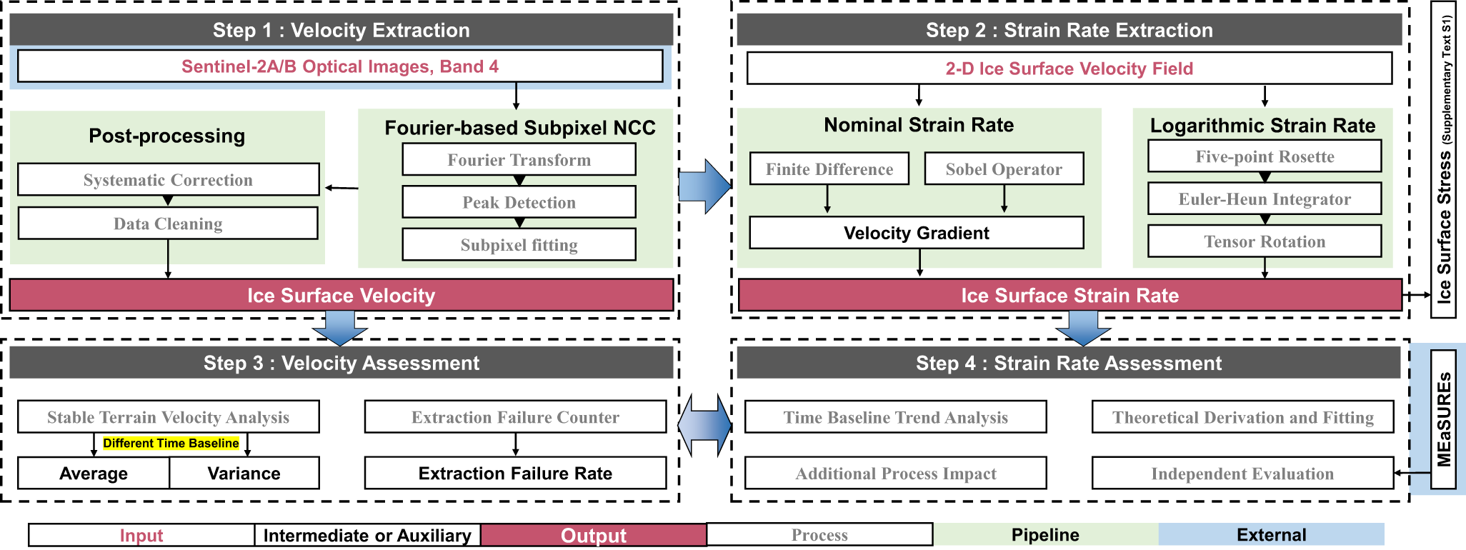
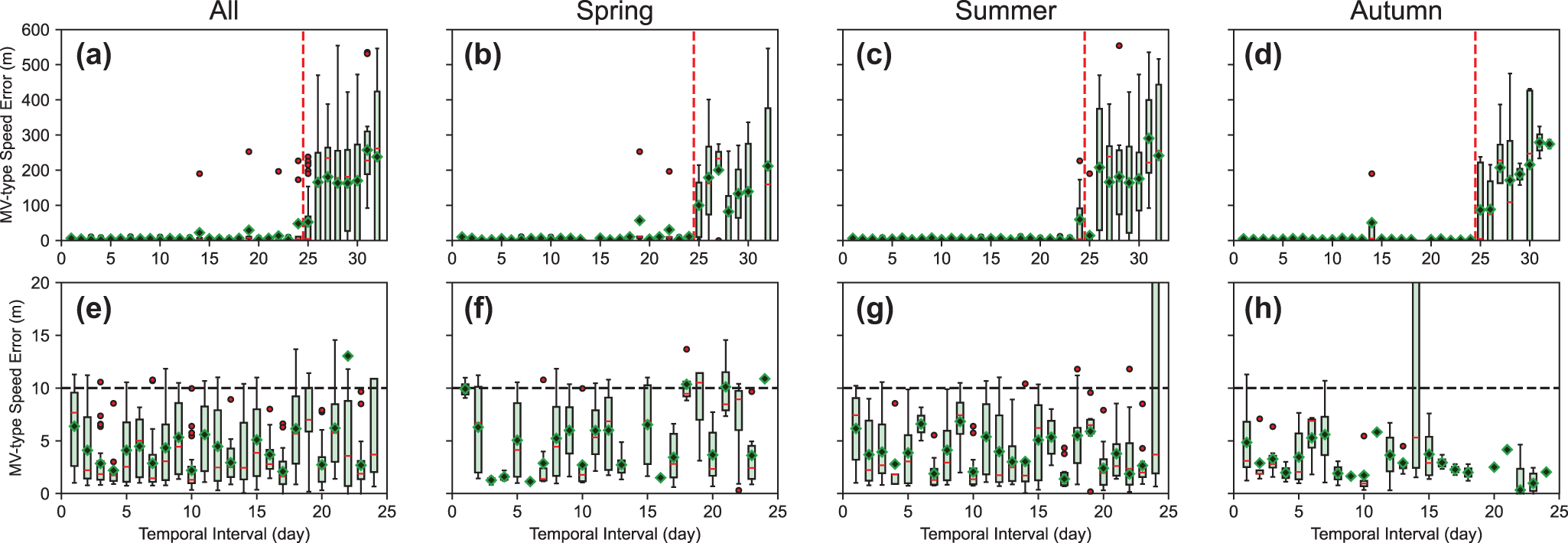


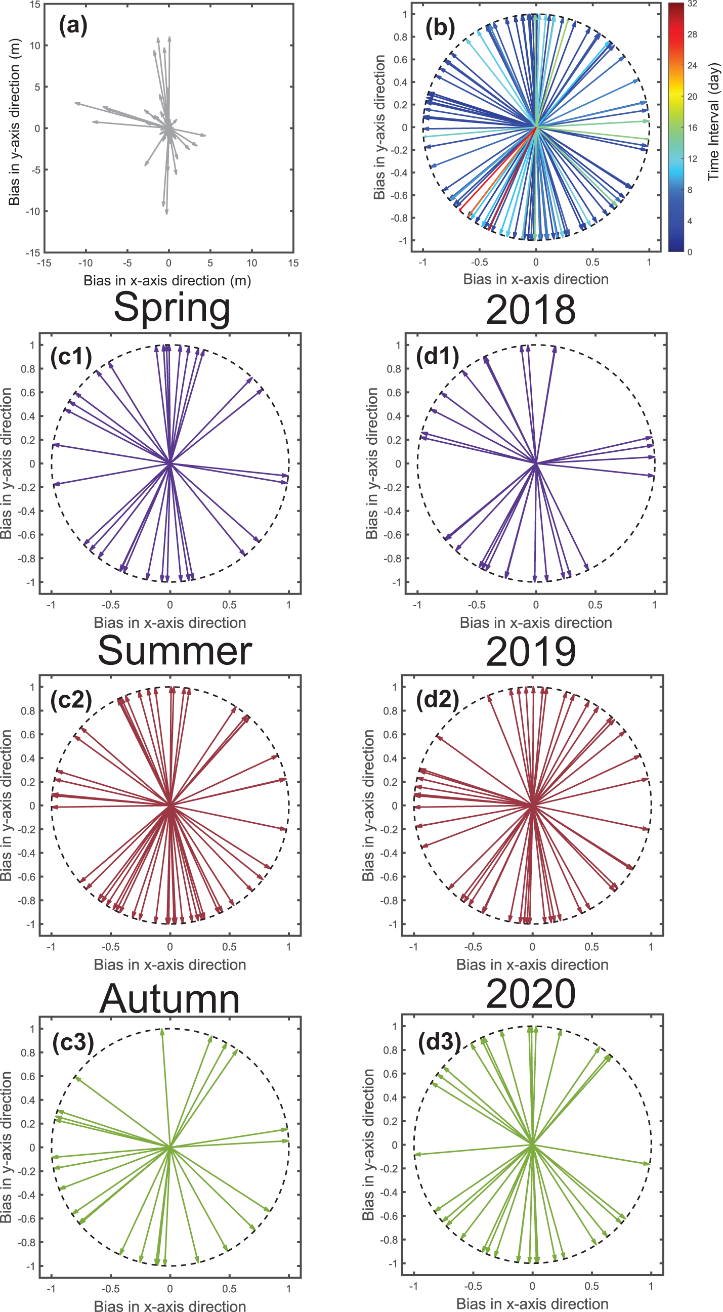
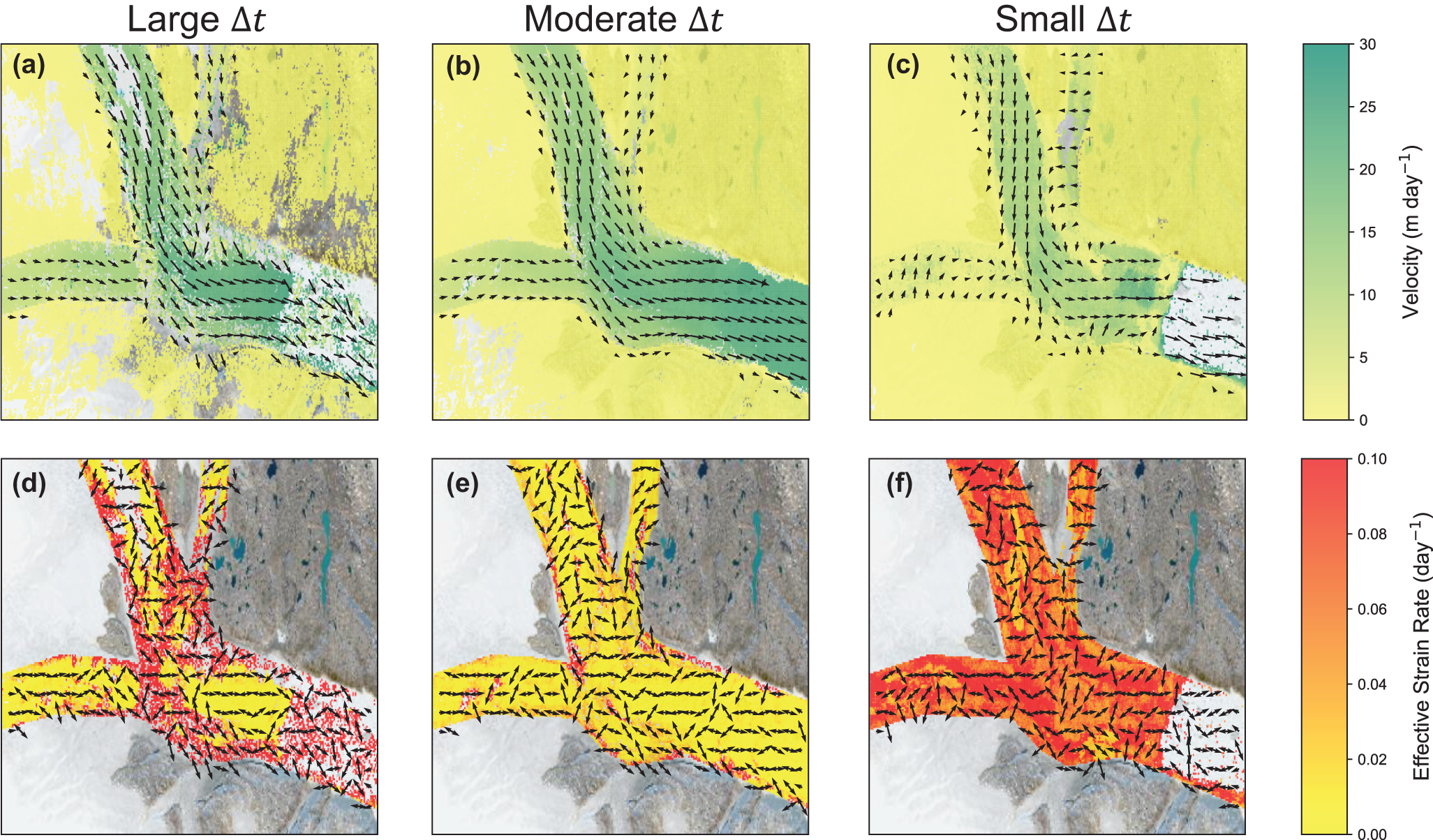


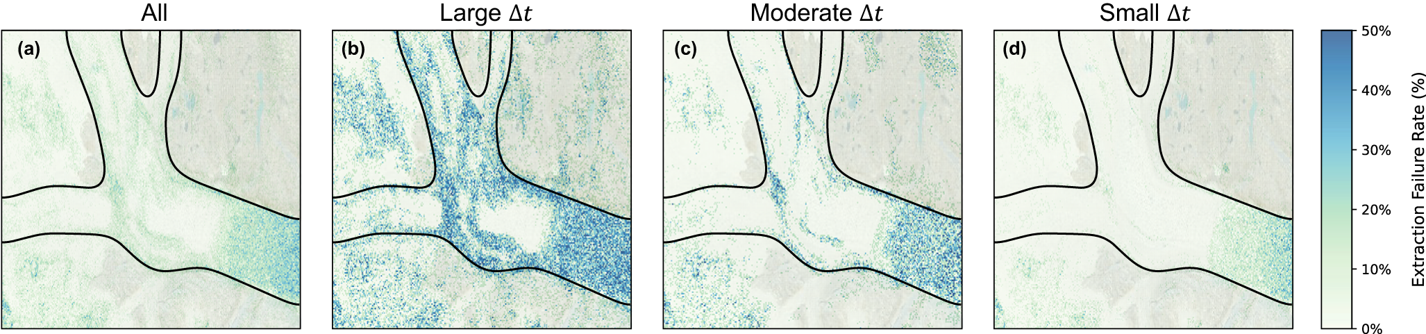


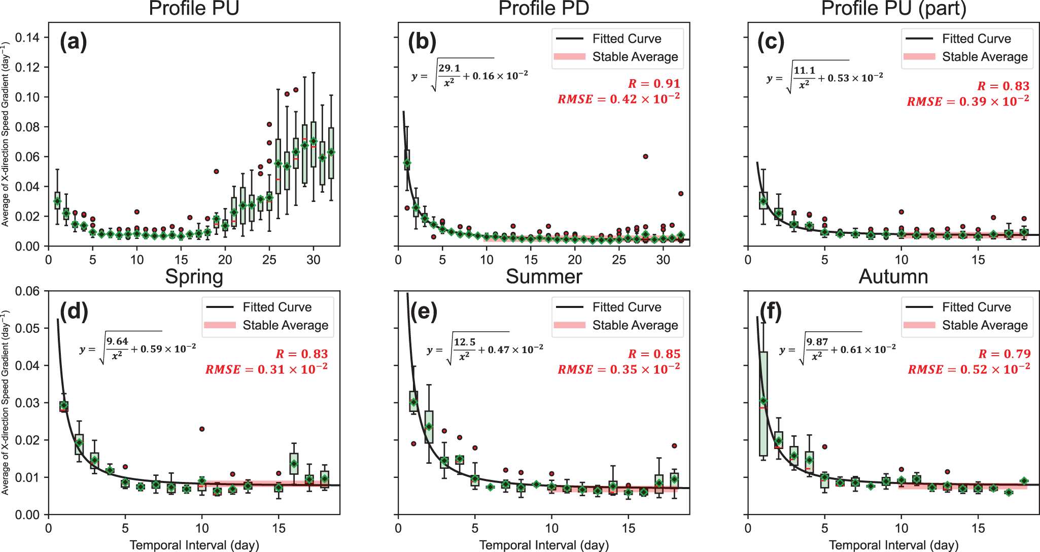


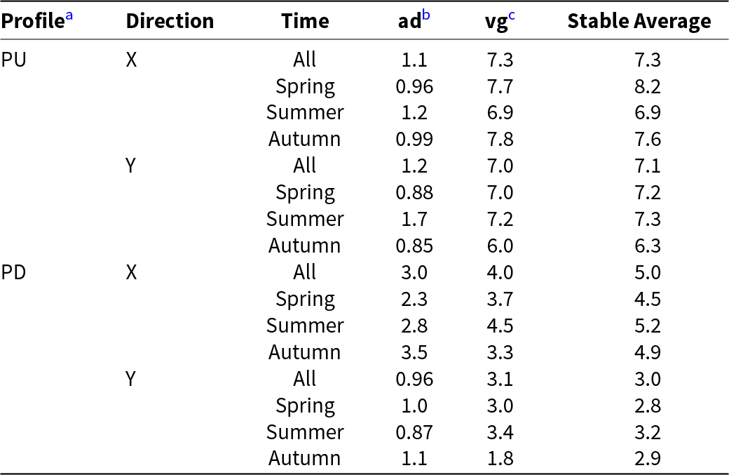

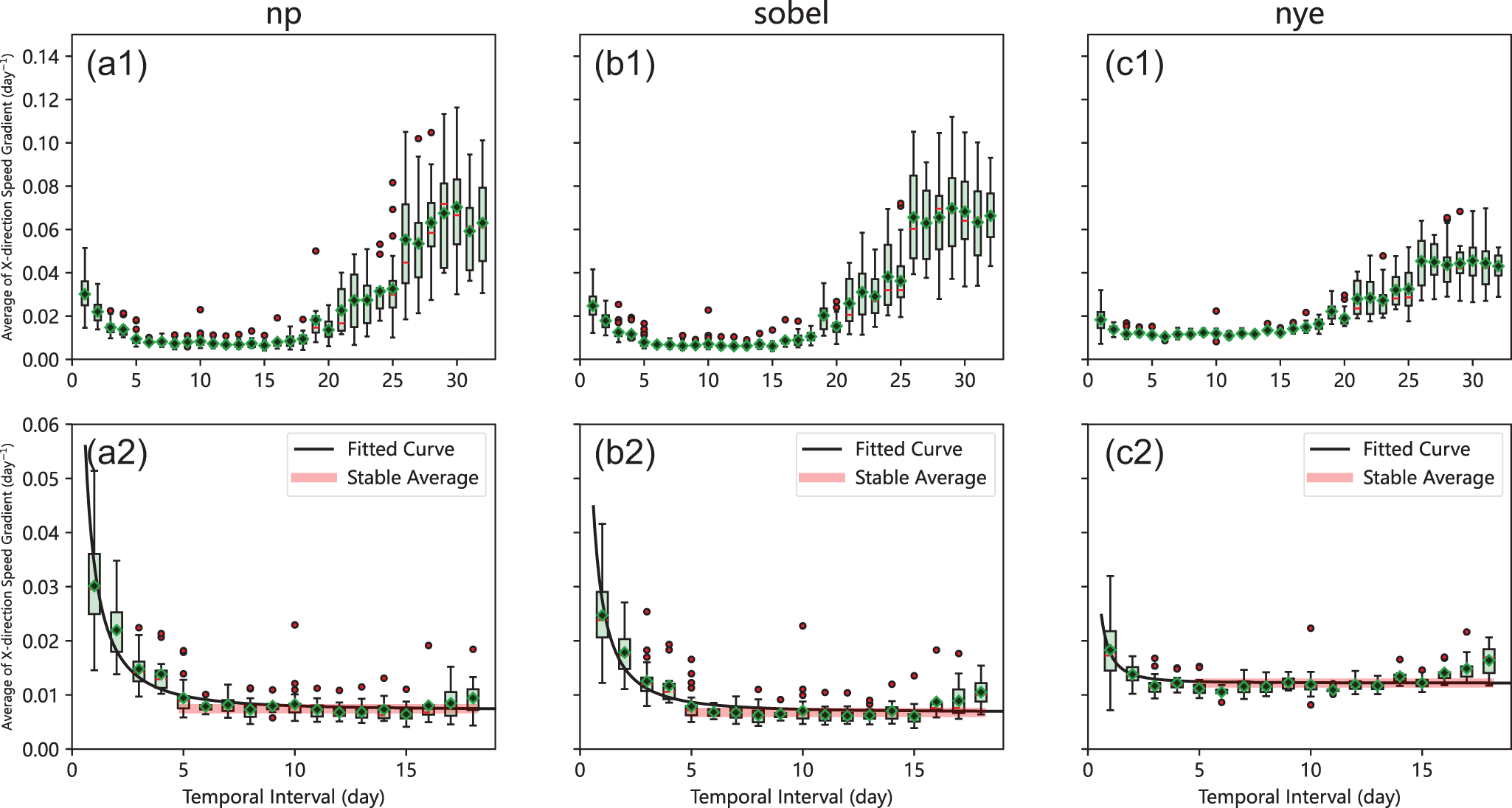


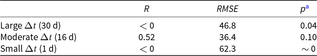


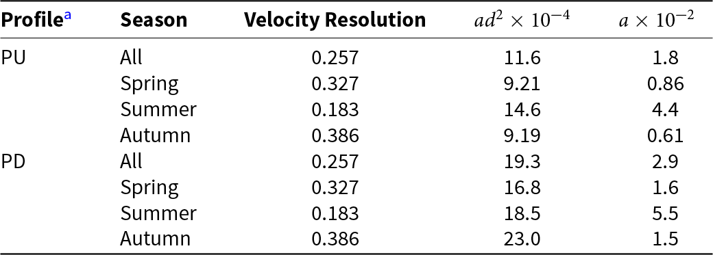


 Open access