


1 Introduction
Dry-snow slab avalanche release is a complex critical phenomenon covering a wide range of scales (Schweizer and others, Reference Schweizer, Jamieson and Schneebeli2003). Across these scales, a sequence of fracture processes results in avalanche release. Dynamic crack propagation through a weak snowpack layer at the slope scale is one of these fundamental processes. Dynamic crack propagation has to be self-sustaining, so that the crack propagates below the slab across the slope; the slab will detach and an avalanche is released, if the slope angle is steep enough that gravitational pull overcomes frictional resistance. In other words, once dynamic crack propagation has started, slope topography and/or crack arrest will determine avalanche release size. Avalanche size is key in estimating the avalanche danger level (Meister, Reference Meister1995; Statham and others, Reference Statham2018; Techel and others, Reference Techel, Müller and Schweizer2020). Reasons for crack arrest can be manifold. From a theoretical point of view, crack arrest occurs when the instantaneous dynamic energy release rate G falls below the dynamic fracture energy Γ (e.g. Freund, Reference Freund1990, p. 394):

Here, G accounts for effects of loading, geometry, bulk material properties, current crack length r, time t and depends explicitly on the crack speed $c = \dot{r}$ (Freund, Reference Freund1990). The dynamic fracture energy Γ, a property characterising the resistance to crack growth, may also depend on crack speed. Analytical solutions providing a dynamic energy release rate for crack propagation in weak snowpack layers are not available, and many of the required material properties remain unknown. What remains, from a theoretical point of view, is the suggestion that crack speed is an important factor which might be related to crack propagation distance.
Deriving an analytical solution for dynamic crack propagation in snow is a far cry, especially since the crack propagation mode is still debated. The crack propagation phase can be seen as a pure shear fracture process (McClung, Reference McClung1979; McClung, Reference McClung1981; Bazant and others, Reference Bazant, Zi and McClung2003; McClung, Reference McClung2021), whereas other studies suggested a mixed-mode anti-crack propagation process (Heierli and others, Reference Heierli, Gumbsch and Zaiser2008; Gaume and others, Reference Gaume, Gast, Teran, van Herwijnen and Jiang2018; Mulak and Gaume, Reference Mulak and Gaume2019; Rosendahl and Weissgraeber, Reference Rosendahl and Weissgraeber2020b). So far, the debate is still open since there is no conclusive experimental evidence for either approach. Moreover, the fracture mode may depend on slope angle (Gaume and others, Reference Gaume, van Herwijnen, Gast, Teran and Jiang2019, Trottet and others, Reference Trottet2021), the orientation of the crack relative to the slope, or possibly snowpack properties. The common fracture modes I–III are well defined for cracks in homogeneous materials, yet snow is a layered material. In snow, cracks generally propagate in thin weak layers, yet the energy required to create new crack surfaces (in the weak layer) stems from the slab layers above the weak layer. Although Eqn (1) defines the balance between energy release (mainly in the slab, source of energy) and energy consumption (mainly in the weak layer, sink of energy), the energy has to be transferred from the source to the sink. Hence, there is an energy flux from the stress–strain field in the slab to the moving crack tip in the weak layer (Broberg, Reference Broberg1999).
The relative magnitude of the strain components in the slab defines the fracture mode and gives rise to the associated wave which transfers the energy through the slab to the crack tip. A crack propagation mode is therefore linked to an elastic wave, and the speed of the crack tip is therefore bounded by the speed of the associated type of wave (Broberg, Reference Broberg1996). Crack speed measurements are therefore crucial, as these may provide an indication of the fracture mode.
Prior to 2000, no field measurements on crack propagation in snow were available. A few observations on whumpfs and firn quakes were published, and these phenomena were described as collapsing waves which can travel over large distances with speeds ranging from 6 m s−1 to slightly slower than the speed of sound in air (Benson, Reference Benson1962; Truman, Reference Truman1973; DenHartog, Reference DenHartog1982). The first crack speed measurement in snow was reported by Johnson and others (Reference Johnson, Jamieson and Stewart2004), who used seismic sensors to measure the snow surface displacement during an artificially triggered, propagating crack in flat terrain, a so-called whumpf. They needed 3 d and numerous field experiments to obtain a single-speed estimate, showing how challenging such in situ measurements are. The mean propagation speed was 20 ± 2 m s−1 over a propagation distance of ~8 m. Since then, numerous studies estimated crack speeds using high-speed photography of propagation saw tests (PST, Fig. 1, upper left), a fracture mechanical field experiment for snow (Gauthier and Jamieson, Reference Gauthier and Jamieson2006; Sigrist and Schweizer, Reference Sigrist and Schweizer2007). Analysing displacements with particle tracking velocimetry provided new insight into weak layer fracture and crack propagation (van Herwijnen and Jamieson, Reference van Herwijnen and Jamieson2005; van Herwijnen and others, Reference van Herwijnen, Schweizer and Heierli2010; Schweizer and others, Reference Schweizer, van Herwijnen and Reuter2011; van Herwijnen and others, Reference van Herwijnen2016b). Reported crack speeds range from 10 to 50 m s−1 (van Herwijnen, Reference van Herwijnen2005; van Herwijnen and Birkeland, Reference van Herwijnen and Birkeland2014; van Herwijnen and others, Reference van Herwijnen2016b). Recently, high-resolution crack speed estimates were obtained with a digital image correlation (DIC) method, highlighting variations in crack speed along a PST and pronounced edge effects (Bergfeld and others, Reference Bergfeld, van Herwijnen, Dual, Schweizer, Fischer, Adams, Dobesberger, Fromm, Gobiet, Granig, Mitterer, Nairz, Tollinger and Walcher2018, Reference Bergfeld2021b).
Overview of methods and scales used to investigate crack speed. Top row: The experimental methods to measure crack speed consisted of a PST, a whumpf and an artificially triggered avalanche, covering distances from <1 m to >400 m. Bottom row: The numerical models used to reproduce these experiments were based on the DEM, the MPM and the FEM.

At scales larger than the typically 2–3 m long PST experiments, van Herwijnen and Schweizer (Reference van Herwijnen and Schweizer2011) derived a speed of 42 ± 4 m s−1 over a distance of 60 m using seismic sensors deployed in an avalanche starting zone. To estimate crack speed, they determined the time between the first arrival of the P-wave and the avalanche release signal and assumed the propagation distance to be the width of the avalanche. Based on videos of avalanches, Hamre and others (Reference Hamre, Simenhois, Birkeland and Haegeli2014) reported several widely varying estimates ranging from 18 to 428 m s−1. For the uncertainty of their speed estimates, they assumed an overall uncertainty on travel distance and travel time but distinct parameters (e.g. image resolution and propagation distance projected onto the terrain) of the individual experiments were not considered. Moreover, uncertainty is reported for a few speed estimates only. Hence, both studies suffer from methodological shortcomings, affecting the reliability of these crack speed estimates.
Overall, the most abundant and reliable data come primarily from PST measurements, raising the question whether the small-scale, rather 1-D PST experiment is representative of the 2-D, large-scale dynamic crack propagation that precedes slab avalanche release.
Performing experiments in avalanche terrain is challenging and often not possible due to safety concerns, so it is a good idea to apply numerical models to simulate this process. Recently, models based on the discrete element method (DEM; Gaume and others, Reference Gaume, van Herwijnen, Chambon, Birkeland and Schweizer2015; Gaume and others, Reference Gaume, van Herwijnen, Chambon, Wever and Schweizer2017; Bobillier and others, Reference Bobillier2020, Reference Bobillier2021) and the material point method (MPM; Gaume and others, Reference Gaume, Gast, Teran, van Herwijnen and Jiang2018, Reference Gaume, van Herwijnen, Gast, Teran and Jiang2019) were developed to investigate crack propagation in snow. Both methods were validated against PST experiments, showing their ability to reproduce crack propagation processes at the scale of a PST. Although these numerical studies also provide new insight into crack propagation at scales beyond the PST scale, validation against slope scale experiments as well as an inter-comparison of both models using the same field experiment is missing.
As outlined before, the speed of cracks propagating in different fracture modes is limited by the speed of different elastic waves (Broberg, Reference Broberg1996) which can be computed from elastic properties and density of the snow. However, the layered snowpack, necessary for crack propagation acts as a waveguide that alters the speed and type of elastic waves travelling within. The finite element method (FEM) can be used to study characteristics of guided wave propagation (Moreau and others, Reference Moreau, Castaings and Hosten2006; Castaings and Lowe, Reference Castaings and Lowe2008; Moreau and Castaings, Reference Moreau and Castaings2008). Such analysis is of great importance for non-destructive testing or health monitoring of engineering structures or the interpretation of seismic signals (e.g. Zhu and Rizzo, Reference Zhu and Rizzo2012; Moreau and others, Reference Moreau2020). Hence, it seems also suitable for investigating wave modes in a layered snowpack.
Given the relevance of crack speed, our aim is to measure crack speed at a range of scales. To this end, we analyse three crack propagation events covering propagation distances from less than a metre up to >400 m. On the snowpack scale, we performed a PST experiment, where a 30 cm wide column is isolated and an artificial cut is introduced within a weak snow layer until crack propagation starts when the critical cut length r c is reached. Close to the PST, we triggered a whumpf, which is essentially a slab avalanche on flat terrain. At the whumpf, we measured crack speed with accelerometers placed on the snow surface. At the largest scale, we analysed a movie of an explosive-triggered avalanche that released at approximately the same time we performed the whumpf and the PST experiments but ~190 km away. Where possible, we reproduced these field experiments with numerical models based on DEM and MPM. To assess the upper limit of crack speeds for different propagation modes and the influence of slab layering, we determined speeds of purely elastic, guided waves with a FE model.
2 Methods
The propagation events we analysed to derive crack speed consisted of a PST, a whumpf and an artificially triggered avalanche, covering distances from <1 m to >400 m and were recorded on 15 January 2019. For each of the events, we subsequently describe the analysis methods and estimate the snowpack properties since these serve as input for the numerical models (Fig. 1).
2.1 Field measurements
At each experimental site, the snowpack was characterised with a manual snow profile following Fierz and others (Reference Fierz2009) (Fig. 2). At the avalanche site, the manually observed profile was taken 2 d after the event and 200 m north of the avalanche in a slope of similar elevation, aspect and slope angle as the avalanche slope.
Manual snow profile showing hand hardness index (width of bars), grain type (colours, see legend) and layer density (black line) for (a) PST, (b) whumpf and (c) avalanche site. Layer density was either measured with a density cutter (black solid line) or was estimated using grain type and hand hardness index (black-dashed line). The depth of the crack in the weak snowpack layer is indicated with the red-dashed lines.

For the PST, the crack propagated in a weak layer consisting of surface hoar (![]() , 10–15 mm) buried at a depth of 1.09 m (Fig. 2a, red-dashed line) below a slab mainly consisting of decomposing and fragmented precipitation particles (
, 10–15 mm) buried at a depth of 1.09 m (Fig. 2a, red-dashed line) below a slab mainly consisting of decomposing and fragmented precipitation particles (![]() ) and rounded grains (
) and rounded grains (![]() ). The crack at the whumpf site propagated at the top and near the avalanche site at the bottom of the weak layer that consisted in both cases of faceted crystals (
). The crack at the whumpf site propagated at the top and near the avalanche site at the bottom of the weak layer that consisted in both cases of faceted crystals (![]() , 1–2 mm, Figs 2b, c; red-dashed lines). Slab thickness was 0.91 and 0.88 m for the whumpf and avalanche, respectively.
, 1–2 mm, Figs 2b, c; red-dashed lines). Slab thickness was 0.91 and 0.88 m for the whumpf and avalanche, respectively.
To investigate variations in snow properties, we also performed snow micro-penetrometer (SMP) measurements at the PST and whumpf site. Generally, the heterogeneity within the PST was small (Fig. 3a) and the SMP measurements were in good agreement with the manual profile. A rather similar snowpack structure was observed at the whumpf site, where we took an SMP measurement at each sensor location; the main differences were a crust just above the weak layer at the whumpf site and the type of weak layer (surface hoar crystals vs faceted crystals). The slab layering, identified in the manual profile (Fig. 2b), was manually transferred to the penetration resistance profiles to track snowpack changes along the crack propagation path (Fig. 3b, background colours).
(a) Penetration resistance measured with the SMP along the PST experiment (blue lines plotted on an image of the speckled side wall of the PST). (b) Penetration resistance measured at each acceleration sensor (indicated by colour as shown in Fig. 4) after triggering the whumpf. The background colours indicate the grain type (top right) of the corresponding layer in the manual profile. Measurements are restricted to the slab to the top of the melt-freeze crust (red layer in Fig. 2b).

(a) Arrangement of the accelerometer sensors at the whumpf site. (b) Measured downward acceleration with time. The time difference Δt of the onsets of acceleration (black dots) between sensor pairs in combination with their spacing Δx were used to compute crack speed.

2.1.1 Propagation saw test
We performed a 5.35 m long PST experiment on a flat and uniform site close to Davos, Switzerland. The experiment resulted in crack propagation till the far end of the beam and had a critical cut length r c = 38 cm. The exposed side wall of the PST was speckled with black ink (Indian Ink, Lefranc & Bourgeois) before the weak layer was cut with a 2 mm thick snow saw. A high-speed camera (Phantom, VEO710) was used to record the speckled wall with an image resolution of 1280 pixel by 352 pixel at a rate of 7000 frames per s (lens aperture: f 2.8, focal length: 24 mm). Camera distortion correction and DIC analysis were performed as described in Bergfeld and others (Reference Bergfeld2021b).
The DIC analysis (subset size: 12 pixels, step size: 3 pixels, smoothing window: 181 frames) of the PST experiment provided us with displacement fields with time. In a post-processing step, we applied a threshold value of 0.05 mm (≈5 times the std dev. of the noise in z-displacement before crack propagation) to the z-displacement to locate the crack tip at each time step (video frame) to derive crack speed, as the slope of linear fits in beam sections, along the PST (beam section width: 50 cm, step size: 5.3 cm). A detailed description of the applied methodology, including uncertainty estimates, is given in Bergfeld and others (Reference Bergfeld2021b).
Snowpack properties: For the PST experiment, slab, weak layer and substratum thicknesses were measured in the manual profile (Fig. 2a). Density of the slab was measured in the field using a 100 cm3 cylindrical density cutter (38 mm diameter) and a vertical resolution of 4 cm (Figs 2a, b; black solid lines). Slab density is given in Table 1 as the mean of all layers attributed to the slab. Uncertainty is assumed to be 5% (Proksch and others, Reference Proksch, Rutter, Fierz and Schneebeli2016). Since density was not measured down to the ground, mean density of the substratum was estimated using a parametrisation on hand hardness index and grain type suggested by Geldsetzer and Jamieson (Reference Geldsetzer and Jamieson2001).
Measured or estimated snowpack properties for the PST, whumpf and avalanche

The columns D, M and F indicate if the property is used as input for the DEM, MPM or FEM simulations, respectively.
The collapse height Δh and the effective elastic moduli of the slab E sl and weak layer E wl were estimated from DIC analysis. Collapse height was taken as the mean of the settlement of the slab measured after crack propagation. For the elastic moduli, 220 displacement fields with an increasing crack length prior to crack propagation were used to compare to displacement fields predicted by the mechanical model established by Rosendahl and Weissgraeber (Reference Rosendahl and Weissgraeber2020a). The optimal set of E sl and E wl was estimated by minimising the residual, with E sl and E wl as free-fitting parameters. Uncertainty is estimated as the std dev. of the scatter over the different cut lengths. For a more detailed description see Bergfeld and others (Reference Bergfeld2021b). Since we did not have direct elastic measures of the substratum, its mean density was used to estimate the elastic modulus. To do so, the density parametrisation of Gerling and others (Reference Gerling, Löwe and van Herwijnen2017) was scaled to fit with our PST measurement:

with the scaling parameter $A = E_{{\rm sl}}^{{\rm PST}} /\rho _{{\rm sl}}^{{\rm PST}}$ . In other words, we forced the density parametrisation to fit our elastic modulus $( E_{{\rm sl}}^{{\rm PST}} )$
 – density $( \rho _{{\rm sl}}^{{\rm PST}} )$
 data point, determined for the slab in the PST experiment. Finally, we used a fixed Poisson's ratio of 0.25 (±0.05) for the slab, weak layer and substratum (Reuter and others, Reference Reuter, Schweizer and van Herwijnen2015).
2.1.2 Whumpf
Crack propagation also occurs on slopes not sufficiently steep to release an avalanche, a phenomenon called a whumpf (Johnson and others, Reference Johnson, Jamieson and Stewart2004). To measure crack speeds in whumpfs, we used custom-designed wireless time-synchronised accelerometers (ADXL362, cut-off frequency: 100 Hz), with a resolution of 10-3g (with g beeing the standard gravity) and a sampling rate of 400 Hz, placed on the snow surface. These sensors measure the acceleration of the slab when a crack in the weak layer passes by (Fig. 4). Although triggering whumpfs is difficult and unpredictable, we performed a successful experiment with seven sensors placed over a distance of 25 m on the same day we performed the PST experiment, and at a distance of 400 m from the PST site.
We aligned the sensors in a straight line and triggered a whumpf by jumping on the snow surface with skis. After the whumpf, we measured the distances between the trigger point and each sensor using a tape measure. With the assumption of circular crack propagation, the crack propagation distance between two sensors Δx was taken as the difference in distance to the trigger point (Fig. 4b). To determine the onset of the acceleration in the ith sensor $t_i^{{\rm onset}}$ (dots in Fig. 4b), we used the Akaike information criterion (AIC; Kurz and others, Reference Kurz, Grosse and Reinhardt2005). The time difference Δt = $t_{i + 1}^{{\rm onset}} -t_i^{{\rm onset}}$
 between two sensors was then used to compute crack propagation speed as c i,i+1 = (Δx/Δt). Uncertainty was assessed by Gaussian error propagation and the contributions from the distance measurement (ux = 0.1 m) and the onset determination. For the latter, a systematic uncertainty was assigned by visually inspecting each AIC automatic onset time on the waveform and comparing it to a manual onset estimate.
The frequency content of the acceleration signals was computed with consecutive Fourier transforms (100 samples each, overlap 90%) using SciPy 1.5.0 (Virtanen and others, Reference Virtanen2020) (Fig. 5). Most of the energy was below 50 Hz, and the median central frequency over all seven recorded whumpf signals was 7.6 Hz.
(a) Downward acceleration (blue line) and displacement obtained by double integration (orange line) with time for sensor 4 at the whumpf site (see Fig. 4). (b) Corresponding spectrogram showing the energy (colours) per frequency band with time.

Snowpack properties: Slab, weak layer and substratum thickness were measured in the manual profile (Fig. 2b) and shown in Table 1. For density, we used a cylindrical density cutter and sampled the slab layers every 4 cm. There were no density measurements for the weak layer and substratum. We thus again used the approach of Geldsetzer and Jamieson (Reference Geldsetzer and Jamieson2001) to estimate its mean density. Since we cannot measure elasticity in the field, mean density of the substratum and slab was used to estimate the elastic modulus using Eqn (2). Values of elastic moduli of weak layers are very scarce in the literature, and we had no possibility to measure it directly. Instead, we assumed the elastic properties to be the same as estimated in the PST experiment. The displacement of the slab was assessed by integrating the acceleration signal twice and forcing the velocity signal (after first integration) to be zero after collapse (Fig. 5a, orange line). The collapse amplitude of the whumpf Δh = 2.2 ± 0.6 mm was taken as the mean of the end displacements of sensors three to seven, since those signals were not influenced by the triggering.
2.1.3 Avalanche
We analysed a video of an explosive-triggered avalanche that released the day we performed the other two experiments. The avalanche released on a steep slope (~40°) above the ski resort of Grimentz, Switzerland (WGS84: 46.1752° N, 7.5200° E), located ~190 km from the field site in Davos. The avalanche was filmed at 30 frames per s and an image resolution of 1920 × 1080 pixel2. For georeferencing surface cracks and avalanche outlines, we analysed selected movie frames with the Monoplotting tool (Bozzini and others, Reference Bozzini, Conedera and Krebs2012) to obtain georeferenced vector data by drawing directly on the image (Fig. 6, left and middle). Transferring the vector data to a GIS system, we then estimated the crack propagation path by taking the line of sight between the trigger point (location of the bombing) and the location where the surface crack opened, whereby visible rocks were bypassed. Crack propagation distance was then computed by projecting the path onto the terrain and computing the distance from the trigger point to the surface crack. The time the crack needed to propagate this distance was estimated from the movie as the lag time between the detonation frame and the frame in which the associated surface crack became visible. Uncertainty of the crack propagation speed u c was computed with Gaussian error propagation and originated from an uncertainty in distance ux = 0.05x (5% of the distance, and at least 5 m) and time ut = 5 frames = 0.17 s.
Schematic diagram showing the work flow for the crack speed estimation based on the movie. (Left) Selected frames from the movie were exported to analyse the position of tensile cracks. (Middle) The Monoplotting tool was used for geo-referencing cracks in the frame. (Right) These geodata were transferred to a map for estimating crack paths and the corresponding projected crack propagation distances (map source: Federal Office of Topography swisstopo).

For each crack propagation path, we further derived slope angle and crack orientation relative to the slope aspect from a digital elevation model (5-m resolution, source: Swiss Federal Office of Topography swisstopo, Berne, Switzerland). A mean slope angle of every crack path was estimated by extracting the slope angle every 3 m along the path. Every 3 m along the path, we also took the azimuths of the crack orientation and the slope aspect. The difference between these two angles was normalised to show if the crack propagated down-, cross- or upslope.
Snowpack properties: Slab, weak layer and substratum thickness are shown in Table 1 and were taken from the manual profile (Fig. 2c). Layer densities were estimated using the approach presented by Geldsetzer and Jamieson (Reference Geldsetzer and Jamieson2001). Applying Eqn (2), we estimated the elastic modulus using mean density of the substratum and slab. Concerning the weak layer, the elastic modulus was again assumed the same as in the PST experiment, and the collapse height Δh = 4 mm was taken as the median collapse height from 192 experiments reported by van Herwijnen and others (Reference van Herwijnen and Greene2016a).
2.2 Numerical models
2.2.1 Discrete element method
Bobillier and others (Reference Bobillier2020) presented a 3-D DEM model to reproduce failure in a layered snow sample. DEM, first introduced by Cundall and Strack (Reference Cundall and Strack1979), is composed of a large number of discrete connected and interacting particles. The PST system was generated using commercial DEM software; PFC3D (v5) (http://www.itascacg.com). For a detailed description of the DEM model for snow, and in particular how particle (and particle contact) parameters relate to macroscopic snow parameters, refer to Bobillier and others (Reference Bobillier2020). Recently, Bobillier and others (Reference Bobillier2021) modelled the PST design and showed that crack propagation in weak snow layers can be reproduced with their DEM model (Fig. 7a). They simulated a 3-D PST consisting of three layers: a basal layer, a weak layer and a uniform slab layer on top. Where available, we used the snow parameters measured in the field (Table 1), otherwise we used the values proposed by Bobillier and others (Reference Bobillier2021) (see Appendix A), obtained by matching simulation and experimental results.
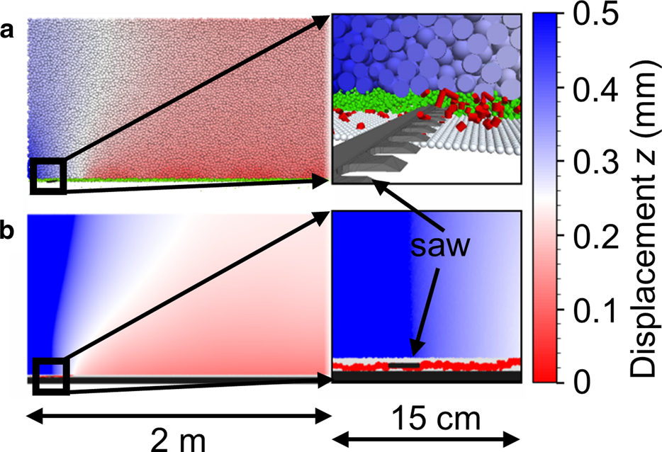
PST setup of the (a) DEM and (b) MPM modelling while sawing the PST. The colouring in the slab indicates the vertical displacement. The insets (15 cm × 15 cm) show a close-up around the saw. The DEM inset (a) shows slab and weak layer particles in blue and green, respectively. Around the saw particles are clipped and bonding damage in the weak layer is highlighted in red. In the MPM inset (b), the crack (red) started propagating and is already ahead of the snow saw.
To derive crack propagation speed, Bobillier and others (Reference Bobillier2021) compared different methods, based on weak layer stress, weak layer bonding damage and slab displacements. They concluded that all methods provide comparable results. In accordance with our field measurement, we used their method based on slab displacements to estimate crack propagation speed in the DEM simulation of the PST. Due to computational limitations the PST is the only field experiment which could be reproduced with the DEM.
2.2.2 Material point method
The MPM method is a continuum and hybrid Lagrangian–Eulerian numerical technique (Sulsky and others, Reference Sulsky, Chen and Schreyer1994), making it particularly well-suited to handle processes involving large deformations and fractures. Snow constitutive models based on critical state soil mechanics (Roscoe and Burland, Reference Roscoe, Burland, Heyman and Leckie1968) were developed to simulate the mechanical behaviour of snow slab and weak snow layers (Stomakhin and others, Reference Stomakhin, Schroeder, Chai, Teran and Selle2013; Gaume and others, Reference Gaume, Gast, Teran, van Herwijnen and Jiang2018). Gaume and others (Reference Gaume, Gast, Teran, van Herwijnen and Jiang2018) reproduced results from different PST experiments, and then applied their model to simulate slab avalanche release on an ideal slope. Here, the numerical setup consisted of a PST with a uniform slab and a weak layer. Particles at the bottom of the weak layer were fixed in position (Dirichlet boundary condition). Details about the constitutive models can be found in Gaume and others (Reference Gaume, Gast, Teran, van Herwijnen and Jiang2018) and Trottet and others (Reference Trottet2021). Where available, we used the snow parameters measured in the field (Table 1), otherwise we used the values which were proposed for snow by Gaume and others (Reference Gaume, Gast, Teran, van Herwijnen and Jiang2018) (see Appendix B), obtained by matching simulation and experimental results. To initiate crack propagation in the simulation, an initial crack of length r was generated in the weak layer by setting the elastic modulus of the associated particles to zero. Quantities of interest, such as the position x or the volumetric plastic strain, were stored for each particle. The crack length was then tracked by defining the crack tip as the location of the furthest plasticised particle, and crack speed c was directly obtained from the temporal evolution of the crack tip position.
2.3 Elastic limits and crack speed estimates
2.3.1 Crack speed estimates
The speed of propagating cracks in snow was estimated by Heierli (Reference Heierli2005) and McClung (Reference McClung2005). Heierli (Reference Heierli2005) proposed an analytical model, suggesting that the crack in the weak layer occurs in the form of a localised disturbance zone (crack tip to the trailing point where the slab rests on the substratum again) propagating as a flexural wave with constant speed $\;c_{{\rm fw}} = \root 4 \of {( g/2h) \;( D/\rho H) }$ where D is the flexural rigidity D = (E slH 3/12(1 − ν 2)), g is the gravitational acceleration, h is the collapse height, ρ is the mean slab density, H is the slab thickness and ν is the Poisson's ratio (0.25 ± 0.05). Basically, Heierli (Reference Heierli2005) followed Johnson and others (Reference Johnson, Jamieson and Stewart2004) who reported a measurement of crack propagation speed in flat terrain and suggested that their measurement should be explained as a flexural wave in the slab. McClung (Reference McClung2005) proposed an alternative explanation for the measurement of Johnson and others (Reference Johnson, Jamieson and Stewart2004) and estimated empirical terminal crack speeds to be in the range c sc = (0.7–0.9)c s where c s is the shear wave speed: $c_{\rm s} = \sqrt {E_{{\rm sl}}/( 2( 1 + \nu ) \rho ) }$
 . Uncertainties for the crack speed estimates are consequently propagated from the uncertainties of the required snowpack parameters (Table 1).
2.3.2 Elastic wave speeds
Calculating the energy flux into the crack tip region leads to upper crack speed limits (Broberg, Reference Broberg1996). For mode I and mode II cracks, the Rayleigh wave speed $c_{\rm r} = (0.87 + \;1.12\nu) {\rm /( }1 + \nu ) \; \cdot \; c_{\rm s}$ is the upper limit (Chi Vinh and Malischewsky, Reference Chi Vinh and Malischewsky2007). If the forbidden subsonic super-Rayleigh region is bypassed in mode II cracking, then the upper limit is the longitudinal wave velocity $c_{\rm l} = \sqrt {E_{{\rm sl}}/\rho }$
 (Broberg, Reference Broberg1996). A mode III crack is limited by the shear wave speed c s. Again, uncertainties are propagated from input parameters. However, the above expressions are valid for waves travelling in an elastic full or half space, whereas the natural snowpack is a layered medium and acts as waveguide.
2.3.3 Finite element method
A snowpack associated with slab avalanche release consists of at least three layers: slab, weak layer and substratum (Fig. 8d). Due to the limited thickness of these layers, the entire system acts as waveguide, affecting wave modes, propagation speed and damping. To investigate which wave modes travel at what speed along the length of the layered slab, FE simulations of wave propagation in a PST-like setup were made with the commercially available software COMSOL Multiphysics. The extent of the model in the x direction was set to 300 m, in order to avoid interferences between the direct wave and unwanted boundary reflections, which would cause resonances of the entire structure. The domain was meshed with squared elements of 1 m in size. The source was defined as a vertical force located at the free surface of the slab, at x = 0 m (Fig. 8a). The source was modelled as 2-cycle Gaussian tone burst with central frequency of 50 Hz. From the energy of the wavefield, different modes can be distinguished (Fig. 8c, e.g. red and blue boxes). In a homogeneous waveguide with only one layer, instead of three, the wavefield consists of a superposition of the so-called Lamb modes. When the frequency is higher than the cut-off frequency of the higher order modes, many modes can propagate at the same time, and the energy of the wavefield splits between the modes, with a distribution that depends on the frequency. When the frequency remains under the cut-off frequencies, only the two fundamental modes propagate in the waveguide. At very low frequencies, the asymptotic behaviour of these two modes can be approximated by a flexural and a longitudinal wave.
Setup of the FEM simulations. (a) The propagation of guided waves in the slab of a PST-like arrangement was simulated by inducing a pulse at x = 0 m and using (b) an elastic modulus profile for the slab layer. (c) The dispersion relations of the different wave modes were used to compute their propagation speeds. (d) Side view of the PST-like FEM configuration consisting of the substratum, weak layer and slab.

In the present case of a waveguide with three layers, however, each layer may act as a waveguide of its own that is coupled with the other two layers. As such, there is co-existence of more than two modes, even from an asymptotic point of view. There is energy exchange between the modes, with a distribution that depends not only on the frequency, but also on the variations of acoustic impedance between the layers. This can be seen for example in Figure 8c, in the region marked with a red box. The frequency-wavenumber branch in this box looks like a flexural mode with a discontinuity ~5 Hz, but the energy of the wavefield is actually split between two co-existing flexural-like modes. The same goes for co-existing longitudinal-like modes, which can be seen in the blue box. The figure also shows branches of higher order modes, with a cut-off frequency ~50 Hz.
For simplicity, we will associate in the following the branches in the red and blue boxes, in Figure 8c, as one flexural and one longitudinal mode, respectively. This approximation can be justified by the motion of these branches, which is flexural and longitudinal. The nonlinearity between the wavenumber and the frequency (Fig. 8c) indicates that the modes are dispersive. Hence different frequencies travel at different velocities. A consequence of this dispersion is that a wave packet centred around a given frequency travels with a group velocity defined by C g = ∂ω/∂k, where ω is the angular frequency and k is the wavenumber. To calculate the group velocity from the frequency-wavenumber spectrum, we proceed in two steps: For each frequency, f n, we find the corresponding wavenumber, k n, by extracting the value of k where the spectrum amplitude is maximum. The group velocity, C g(f n) around the nth point (f n, k n) in the spectrum, is finally approximated numerically such that

In most models, also in the DEM and MPM models, the slab is treated as a uniform layer with an isotropic effective elastic modulus and a mean density. In nature, the slab generally has a pronounced layering. In the density profile (Fig. 8b), we visually identified six sections where density approximately changed linearly with depth (black line in Fig. 8b), and converted those into a section-wise elastic modulus profile using Eqn (2) (red line in Fig. 8b).
To highlight the influence of slab layering on wave speed, we performed two simulations, one with a uniform slab and one with a layered slab. In addition, we investigated the influence of weak layer properties on crack speed by varying the elastic modulus of the weak layer (0.4, 0.6 and 1 MPa). In total, we performed six FEM simulations.
3 Results
We derived crack propagation speeds from three crack propagation events recorded on the same day. These experimental values were compared to results of numerical models established to reproduce crack propagation in weak snow layers (DEM and MPM) or to assess elastic wave speeds in the slab (FEM).
3.1 Field measurements
In the PST, crack propagation started with an initial speed of 17 m s−1 in the first metre and increased thereafter (Fig. 9a, blue line). Crack speed peaked at x = 4.5 m with 58 m s−1, and overall the mean speed was 39 ± 13 m s−1. In the whumpf experiment, crack speed was computed for different sensor combinations. The two sensors closest to the trigger point could not be used, as the signal also contained noise from jumping on the snow (Fig. 4b, blue and orange lines). Also, we did not compute the speed between sensors 6 and 7, as these were at a very similar distance from the trigger point (Fig. 4a, brown and violet sensors). In total, we thus had nine pairs to calculate crack speed (Fig. 9a, orange dots), with a mean speed of 49 ± 5 m s−1. In the avalanche movie, we analysed 14 crack paths, resulting in crack propagation speeds between 23 and 44 m s−1 (mean: 36 ± 6 m s−1) covering distances from 26 to 440 m (Fig. 9a, green squares). Crack propagation paths were located on slopes with mean slope angles between 32° and 42° and there was no link between slope angle and crack speed (Pearson's r = −0.51, p = 0.05; Fig. 9b). Since the explosive was placed near the ridge, there was only one upslope crack path, whereas all others were cross-slope or downslope. Again, there was no clear link between propagation path and crack speed (Pearson's r = −0.13, p = 0.63; Fig. 9c).
(a) Crack speed with propagation distance for the PST (blue), the whumpf (orange) and the avalanche (green). For the PST, the red area behind the blue curve indicates the uncertainty. For whumpf and avalanche, the uncertainty is given with red error bars. The grey horizontal lines behind the whumpf speeds indicate the distance range used to compute the respective data point. (b) Crack propagation speed for the avalanche with mean slope angle and (c) with crack orientation relative to the slope aspect. Each dot represents a speed estimate from a cracking path while the bars show the uncertainty.

3.2 Numerical modelling
Both the DEM and the MPM simulations reproduced the right order of magnitude as well as the overall trend in crack speed along the PST experiment. Although values obtained with the DEM model underestimated crack speed compared to the experiment, the MPM model overestimated crack speed. Away from the PST beam ends (2 m < x <4 m), where edge effects are small (Bergfeld and others, Reference Bergfeld2021b), mean speeds were 44 ± 6, 31.6 ± 2.1 and 63 ± 3 m s−1 for the experiment, DEM and MPM, respectively.
At the whumpf scale, we used two different MPM geometries. First, we modelled a 3-D PST-like beam configuration (width: 0.3 m, length: 25 m, labelled as ‘MPM-beam’ in Fig 11a). Second, we modelled a 3-D flat area of 25 m by 25 m (MPM-areal in Fig. 11a). Model geometry had no influence on crack propagation speeds, as mean speeds were 54 ± 2.2 and 56 ± 1.6 m s−1 for the areal and beam configuration, respectively, in good accordance with the field measurements (49 ± 5 m s−1).
The avalanche was also modelled using two different MPM configurations. First, we simulated a cross-slope PST-like beam configuration (width: 0.3 m, length: 25 m, slope angle: 40°, labelled as ‘MPM-beam’ in Fig. 11b). Second, we modelled a tilted area (40°) of 25 m by 25 m and computed the cross-slope crack propagation speed (MPM-areal in Fig. 11b). The beam configuration resulted in a fairly constant speed of $\bar{c}$ = 48 ± 4 m s−1, in the same range as the speeds derived from the movie. The slope simulation showed a steady increase in speed (Fig. 11b, purple solid line), without reaching a steady state within the 25 m of the model domain.
3.3 Elastic limits and crack speed estimates
Elastic wave speeds were in the range of 103 ± 6 to 224 ± 35 m s−1 (Table 2). As expected, they were generally much higher than the experimental crack propagation speeds. McClung (Reference McClung2005) estimated a realistic range for weak layer crack speeds to be c sc = (0.7–0.9)c s which would lead to c sc ∈ [79, 127] m s−1 and therefore around double the experimentally estimated crack propagation speeds. The estimate for crack speed c fw as suggested by Heierli (Reference Heierli2005), agreed well with the experimental crack propagation speeds c exp (Table 2).
Theoretical wave speeds for the PST, whumpf and avalanche

The longitudinal wave speed cl, the shear wave speed cs and Rayleigh wave speed cr of the slab was computed from snow properties. The three columns on the right show crack propagation speed estimates. To calculate csc and cfw, the formulations by McClung (Reference McClung2005) and Heierli (Reference Heierli2005), respectively, were used. In the last column, the experimental crack speeds cexp are listed for comparison.
In our FEM analysis, the PST-like beam configuration, consisting of slab, weak layer and substratum, acts as a waveguide with multiple layers. We determined the group velocity of the flexural and the longitudinal wave modes for different weak layer elastic moduli, as well as with and without slab layering. The flexural wave speed c f increased up to ~30 Hz (120 m s−1), and decreased thereafter (Fig. 12a). At higher frequencies (f > 35 Hz), the decrease was more pronounced for a layered slab (compare dashed and dotted lines in Fig. 12a). In the region of interest, at a dominant frequency of 7.5 Hz, group velocities for the flexural mode ranged from c f = 95 to 105 m s−1, indicating that the elastic modulus of the weak layer as well as slab layering had little influence on flexural wave speeds.
Overall, longitudinal wave speeds were much higher at low frequencies (f < 35 Hz) than flexural wave speeds. Weak layer elastic modulus did not influence the longitudinal wave mode. However, longitudinal wave speeds were somewhat sensitive to slab layering in the lower frequency range. Longitudinal wave speeds at 7.5 Hz were in the range of 370–380 m s−1 for the layered slab and 440–470 m s−1 for the uniform slab.
4 Discussion
We presented crack speed measurements from three crack propagation events covering a wide range of scales and compared these to theoretical wave speed limits and results of numerical simulations. Overall, our measurements of crack speed from the PST, whumpf and avalanche slope provided similar values, although there were some differences between the different propagation events (Fig. 9). We did not observe a dependence of crack speed on propagation distance, suggesting that crack propagation in the whumpf experiment and the avalanche had a fairly constant speed, ~49 and ~36 m s−1, respectively.
Determining crack speed always requires tracking the crack tip. Hence, any method to estimate the crack tip potentially affects crack speed estimates. In our flat field experiments, PST and whumpf, we estimated the location of the crack tip using vertical displacement and acceleration, respectively. The main source of energy for crack propagation stems from the vertical displacement of the slab, since horizontal displacement does not free any energy (e.g. gravitational potential energy or mechanical energy stored in the slab). Hence, the crack tip speed has to be in line/synchronous with the speed the vertical displacement travels along the slab. Therefore, crack speed estimates derived from vertical displacement and acceleration in flat field experiments provide accurate estimates, even if the tracked location does not necessarily coincide with the exact location of the crack tip. Hence, the methods to determine crack speed are robust in the case of the PST and whumpf, the crack speed in the avalanche, however, could be greater than our methodology revealed. It remains an open question if slab fractures, visible at the snow surface, are good proxies for the location of the crack tip in the weak layer. Indeed, it is entirely possible that the crack in the weak layer has already propagated further before a crack in the slab becomes visible on the images. We considered three possible processes (Appendix C) that could result in a delay between the appearance of slab fractures and the passing of the crack tip in the weak layer, resulting in lower crack speed estimates. However, as the processes are presumably constant, the influence on crack speed decreases with increasing propagation distance. By accounting for these delays, we more accurately estimated the terminal crack speed (45 ± 5 m s−1), which was still close to the uncorrected estimate (36 ± 6 m s−1).
Since similar experimental crack speeds were observed throughout the three crack propagation events, it can be assumed that crack propagation processes observed in the PST were similar to those in the whumpf and the cross-slope propagation in the avalanche. The increase of crack speed in the first 2 m of the PST beam highlights the need for long PST experiments, at least longer than the so-called touchdown distance, which is typically 2–3 m (Bair and others, Reference Bair, Simenhois, van Herwijnen and Birkeland2014; Bergfeld and others, Reference Bergfeld2021b). If this is fulfilled, our results suggest that crack propagation in a PST is representative for larger 2-D crack propagation occurring in whumpfs and for the cross-slope direction in our avalanche movie. Long PST experiments may thus be well suited to investigate self-sustained crack propagation.
On the PST scale, the numerical simulations (MPM and DEM) reproduced the initial increase in crack speed well. In general, the DEM method underestimated crack speed compared to the experiment, whereas the MPM method resulted in higher values (Fig. 10). The discrepancy of the crack speeds between the MPM and DEM methods could stem from the different implementations how damping is realised in the models. In MPM, no explicit numerical damping is used at the level of the balance equations and the constitutive model is rate-independent. A small amount of damping is introduced during the interpolation between the grid and the particles (see Gaume and others (Reference Gaume, Gast, Teran, van Herwijnen and Jiang2018) for more details) but does not affect the presented results. In contrast, in DEM, a global damping coefficient of 0.6 (Cundall and Strack, Reference Cundall and Strack1979) was used in Newton's equations.
Crack speed estimates for the PST. The DEM (brown line), the MPM (purple-dashed line) and the field experiment (blue) showed a strong increasing crack speed at the beginning of crack propagation before crack speed increased less in the centre part of the PST beam.

Crack speed with propagation distance for (a) the whumpf and (b) the avalanche. The orange (whumpf) and green (avalanche) dots show the experimental values. MPM simulations were either performed using a PST-like beam configuration (MPM-beam, purple-dashed line) or for a 3-D area of 25 m by 25 m (MPM-areal, purple solid line).

Group velocities of (a) the flexural wave mode and (b) the longitudinal wave mode with frequency. Simulations with a uniform effective elastic modulus for the slab are shown as dashed lines, whereas the crosses indicate a layered slab with varying elastic modulus as shown in Figure 8b. Different values for the elastic modulus of the weak layer are depicted in black, red and blue.

The DEM method is computationally very costly (the PST took ~1 d on a 14 cores Intel Xeon CPU with 256 GB RAM) and is therefore currently limited to the PST scale. The MPM method, in contrast, can also be used to perform simulations for geometries larger than the PST, provided certain requirements are fulfilled. Currently, the mesh size has to be the same for the modelled system containing slab and weak layer. Resolving processes in the weak layer therefore requires a mesh size smaller than the weak layer thickness. Reducing the mesh size was computationally too costly. Instead we modelled the weak layer with a thickness of 45 cm rather than the 1.5 cm observed in the manual profile (see Appendix B). Since the thickening of the weak layer affects the stiffness of the weak layer, we scaled the elastic modulus of the weak layer accordingly to keep the stiffness constant. Doing so, the measured crack propagation speed in the whumpf was fairly well reproduced, independent of the MPM model geometry (Fig. 11a). This MPM result further suggests that the PST-like configuration, which is rather 1-D, is representative of 2-D crack propagation in flat terrain as observed in whumpfs.
For the avalanche slope, we again tested two MPM model configurations, with very different outcomes. Here, the crack speed of the areal configuration increased with propagation distance and did not reach a terminal speed within the 25 m (Fig. 11b, purple solid line). Hence, in the areal configuration the MPM model predicted a different crack propagation speed behaviour than derived from the avalanche video, probably, because the crack in the areal MPM simulation propagated in Mode III. In contrast, an increasing crack speed with propagation distance was not observed for the cross-slope, beam like MPM configuration (Fig. 11b, purple-dashed line), which resulted in similar crack speeds as derived from the avalanche video. Most likely this is due to the downside support of the beam, which we added to force the cracking in a pure flexural mode similar to in the whumpf and PST experiment, where mode III does not occur.
Therefore, we assume that the cross-slope crack propagation observed in our avalanche movie is not influenced by the slope angle, which potentially could change crack propagation into pure mode III. Possibly, consecutive slab fractures behind the crack tip hinder this transition into mode III. In the areal MPM simulation, the slab is not allowed to fracture and consequently showed this transition, indicated by the increasing crack speed. Another factor which may have prevented the transition into mode III in our avalanche movie could be the natural supporting effect from the foot of the slope. Gaume and others (Reference Gaume, van Herwijnen, Gast, Teran and Jiang2019) used MPM to simulate crack propagation in a full slope, which reached flatter areas as well, and did not report an increasing crack speed in the cross-slope direction. In contrast, our areal MPM configuration had a uniform slope angle and was truncated at the model boundaries; hence, downside support was not possible for geometrical reasons. The mismatch between crack speeds from the avalanche movie and our MPM simulation suggests that more research is needed to understand the influence of slope angle in the MPM model, and similarly, more field data are needed to see whether our single measurement is representative.
With the exception of the latter mismatch, we can say that the MPM- and DEM-derived crack speeds are in reasonable agreement with the measurements. However, given the large number of input parameters in the models, and that some of these parameters cannot (or only imprecisely) be measured in the field, a sensitivity study would be required to add some uncertainty to the model results, but this is beyond the scope of the present study.
Furthermore, we compared our experimental crack speeds to the speed of body waves in infinite media and to two models predicting crack speed in relation to slab avalanche release (Table 2). Only the formulation suggested by Heierli (Reference Heierli2005) agreed well with experimental values, whereas the crack speed range suggested by McClung (Reference McClung2005) and the body wave speeds were substantially higher. Of course, the latter is expected since typical maximum crack speeds of other materials are typically <60% of the corresponding wave speed (Broberg, Reference Broberg1996).
As crack propagation preceding avalanche release occurs in a layered medium, we also performed FEM simulations to identify speeds of different wave modes as elastic limits for crack propagation in snow. Such a system can be seen as a waveguide which introduces geometric dispersion. In that case, the group velocity carries most of the energy and is dispersive (i.e. frequency dependent). A spectral analysis of the observed whumpf signal showed that most of the energy of the propagating crack was below 50 Hz (Fig. 5), with a median peak in the spectrum ~7.5 Hz. This is in good agreement with the spectral content of seismic signals generated by crack propagation before slab avalanche release (van Herwijnen and Schweizer, Reference van Herwijnen and Schweizer2011). Evaluating the FEM simulated group velocities at 7.5 Hz, the measured crack speed was ~0.4 times the flexural wave speed, whereas it was only 0.1 times the longitudinal wave speed.
It has been known for a long time that cracks tend to accelerate to a constant (terminal) speed (Schardin, Reference Schardin, Averbach, Felbeck, Hahn and Thomas1959), which is lower than the elastic wave speed that corresponds to the crack propagation mode (Broberg, Reference Broberg1996), i.e. the elastic wave speed is an upper limit. This restriction originates from the energy flux into the dissipative region, namely the crack tip. The energy flux decreases with increasing crack speed, and it goes down to zero at the limiting speed (Freund, Reference Freund1990; Broberg, Reference Broberg1996). In the avalanche case, the available energy stems from the work of gravity released by the slab, then the energy is transferred by the slab to the moving crack tip within the weak layer. Therefore, the crack propagation speed is limited by an elastic wave mode of the slab. Since the PST and whumpf experiments were performed on flat terrain, we assume that the energy available for crack propagation stems from flexural slab bending due to weak layer collapse. Since for self-sustained crack propagation the crack tip cannot propagate faster than the energy source, we suggest that the flexural wave speed is an upper bound for the crack speed on flat terrain. This also explains why the formulation of Heierli (Reference Heierli2005) agreed very well with our measurements, as it is essentially a formulation for a flexural wave. In other words, if the fracture mode is a mixed mode anticrack (Heierli and others, Reference Heierli, Gumbsch and Zaiser2008), its limiting speed is given by the flexural wave speed in the slab c f. In our experiments, the speeds were c ≈ 0.4c f.
The similarity of the crack speed measured in the avalanche experiment suggests that crack propagation on the slope did not change the mode of propagation, whereas tilting the model geometry changed the mode in the MPM simulation. That the fracture mode did not change is also supported by the fact that we found neither a dependence of crack speed on crack orientation nor on slope angle (Fig. 9). However, these observations are based solely on the results from one single avalanche. We do not demonstrate that other fracture modes do not exist in nature. In particular, for distant triggering through steep slopes, gravitational tensile stress might favour the crack propagation in modes II and III, and crack propagation at greater speeds than observed in our single measurement might occur as suggested by recent modelling results (Gaume and others, Reference Gaume, van Herwijnen, Gast, Teran and Jiang2019; Trottet and others, Reference Trottet2021). Clearly, future measurements are needed to confirm this interpretation.
Our FEM analysis further revealed that slab layering did not overly influence the flexural wave speed and therefore, probably had a little effect on the crack propagation speed. This is of particular interest since the slab is most often treated as homogeneous. Another parameter hard to determine in the field is the weak layer elastic modulus, and its influence on the flexural wave speed was also very limited.
5 Conclusions
We presented three examples of crack speeds in weak snowpack layers determined from field experiments and observations, and compared these to results from numerical models and elastic wave speeds. Crack propagation speed is a highly relevant driver of dry-snow slab avalanche release size.
The three propagation events (PST, whumpf and avalanche) occurred on the same day in similar snowpacks and cover a range of distances from <1 m to >400 m, hence the scales relevant for slab avalanche release. The speeds ranged from 39 to 49 m s−1, which are remarkably close in view of the natural variations in the different parameters, e.g. the slab thickness. The similar speeds obtained for different distances and geometries allow the assumption that crack speed measurements obtained from PST experiments may be representative of slope scale crack propagation, provided the columns are long enough, ideally >5 m. Crack speeds modelled with DEM and MPM were in the same range as the experimental values. The MPM simulation for a tilted area of 25 m × 25 m revealed a steadily increasing crack speed, which was not observed in our single avalanche event. The comparisons also showed some discrepancies, demonstrating the need to better understand the link between model results, model input parameters and how these relate to snowpack properties.
Using an FEM model, we determined the dispersive speeds of different guided wave modes. The crack speeds we obtained corresponded to ~0.4 times the flexural wave speed at 7.5 Hz, the dominant frequency in signals measured during crack propagation with wireless accelerometers. The FEM results further suggest that slab layering and weak layer elastic properties may have little influence on wave speeds at this frequency.
Our measurements of crack speed at various scales are limited, yet they are consistent with the assumption that crack propagation in weak snowpack layers, at least in flat terrain, is linked to the flexural wave mode in the slab in the same way that a mode II crack in other materials is generally linked to elastic shear or longitudinal waves. Measurements on steep slopes and in different snowpacks, as well as comprehensive modelling approaches, are still needed for solid conclusions on the dominant fracture modes in dry-snow slab avalanche release.
Data
Underlying data are available on EnviDat: 10.16904/envidat.250. (Bergfeld and others, Reference Bergfeld2021a).
Acknowledgements
We thank Laurent Crettenand for capturing the video of the avalanche. We are also grateful to Augustin Rion and Armand Salamin who recorded the corresponding snow profile. Furthermore, we thank the reviewers, Pascal Hagenmuller and Karl Birkeland for their positive and constructive comments that helped to improve the manuscript. BB and GB were supported by a grant from the Swiss National Science Foundation (200021_169424).
Author contributions
JS, AH and BB designed the research before BB and AH conducted the field experiments. GB performed the DEM simulations, BT and JG made the MPM simulations and LM together with EL did the FEM analyses. JC helped to geo-reference the avalanche movie. JD and JS contributed to all parts of the project. The manuscript was written by BB with input from all co-authors.

Appendix B: Input parameters for MPM simulations
See Table 4 on the next page.
MPM input parameters

Appendix C: Error assessment for the crack speed estimates obtained from the avalanche video
Crack speed estimates from the avalanche video may be subject to systematic errors. To estimate crack speed, we tracked slab fractures that progressively became visible on the video images. With this method, we thus assumed that slab fractures are a good proxy for the location of the crack tip in the weak layer. However, there are three processes that can result in a lag between the appearance of the slab fracture and the actual location of the crack tip, and thus consistently lower crack speed estimates. First, at the trigger point, the explosive likely destroys the weak layer over an area that extends several metres beyond the explosion. Thus, crack propagation does not start at x = 0 m but rather at x = x 0 (a). Second, a slab fracture may only start to form when the crack in the weak layer has already propagated a distance x 1 further. Third, there is a delay between the formation of the slab fracture and the first time it becomes visible on the images (x 2).
Since the contributions x 0 and x 1 are unknown, we assumed these to be constant and combined them x ′ = x 0 + x 1 (Fig. 13). To estimate x 2, we assume that a slab fracture becomes visible when it reaches a size of one full pixel on the image x vis = 1 pixel. The time t vis needed for a slab fracture to open this distance can be estimated as:

with g the gravitational acceleration, $\theta = 39^\circ$ the mean slope angle and μ = 0.57 the frictional resistance (van Herwijnen and Heierli, Reference van Herwijnen and Heierli2009) after weak layer cracking.
(a) Estimating the crack tip location may include systematic errors due to the explosive (x 0), a potential difference between slab fracture formation and crack tip (x 1) and the time a slab fracture needs to become visible (represented with the distance x 2). (b) Crack speed measures from the avalanche movie (green squares) and the interpretation of these data with the simple model from Eqn (C1) (solid lines). In orange we forced the unknown xʹ to be xʹ = 0 m, and estimated true crack speed c, whereas in blue we estimated both parameter from the measurements.

Once the slab fracture opening time t vis is estimated, the error x 2 is estimated as x 2 = c t vis, where c is the crack speed in the weak layer. Finally, we assume constant crack speed in the weak layer and interpreted our measured data pairs t m, x m with a simple model accounting for the uncertainties x 2 and x ′:

where t m and x m are the initial estimates for crack propagation time and distance leading to the crack speed measures (green squares in Fig. 13). First, we neglected the contributions of x ′, and just optimised (in a least squares manner) crack speed c in Eqn (C1) with our data pairs t m, x m (Fig. 13b, orange line). This results in a weak layer crack speed of c = 43 ± 8 m s−1. Second, we also accounted for the error x ′ (Fig. 13b, blue line). This additional degree of freedom in the model had a little influence on the crack speed (c = 45 ± 5 m s−1) and x ′ was estimated to be ${x}^{\prime}\;\approx 15\,{\rm m}$ .
.
This simple model provides a plausible explanation for the observed initial increase in crack speed. However, the assumption of a terminal crack speed cannot be validated. For larger distances, this assumption is supported by our data, as crack speed estimates were relatively constant, and this is the range where the relative influence introduced by the error contributions becomes negligible (e.g. relative deviation against terminal speed c(x > 200 m) ⩽5%).


 Open access