2.1. Generality and description of the event

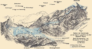
The Altels (Berner Oberland, Switzerland) summit is 3629 m a.s.l. and has a pyramidal shape. The northwestern flank is 1500 m high with a 35–40° slope (Fig. 1). It consists of relatively smooth malm limestone (see Fig. 3). In the mid-19th century, this face was largely covered with an unbalanced ramp glacier (i.e. the snow accumulation is mostly compensated by break-off; Reference Pralong and FunkPralong and Funk, 2006), located between 3629 and 3000 m a.s.l. In the early morning of 11 September 1895, a large part of the glacier broke off and tumbled down. This icefall lasted ∼1 m in and the accompanying thunder could be heard in Kandersteg (∼10 km away). Many people thought it was an earthquake. This catastrophic break-off was carefully described and reported by Reference ForelForel (1895), Reference HeimHeim (1895) and Reference Du PasquierDu Pasquier (1896) and, later, by Reference Röthlisberger and KasserRöthlisberger (1981).

Fig. 1.

Overview of Altelsgletscher, 25 November 1894, 10 months before the glacier broke off. (Photograph: P. Montandon from Englistliggrat, 2665 m a.s.l.)

The volume of the break-off was estimated as 4 × 10⁶ m³, which is the largest known glacial fall in the Alps. The resulting ice avalanche ravaged the high mountain pasture situated underneath (the Spittelmatte) and killed six people and 170 cattle. Due to its high velocity (430 kmh⁻¹ (Reference HeimHeim, 1895; Reference Röthlisberger and KasserRöthlisberger, 1981)), the avalanche piled up to 300 m on the opposite slope, towards the Üschinengrat (Fig. 2). An area of ∼1 km² of the pasture was buried under an ice layer 3–5 m thick. As Reference ForelForel (1895) reported, a similar event had occurred at the same place in 1782, killing four people and hundreds of domestic animals (Reference Raymond, Wegmann and FunkRaymond and others, 2003). Reference ForelForel (1895) pointed out that the 1895 summer was warmer than usual. The event is unlikely to occur again, because Altelsgletscher has almost disappeared (a tongue remains on its left side, which will melt away in the near future; Fig. 3a).

Fig. 2.

General overview of the event (after Reference HeimHeim, 1895).

Fig. 3.

(a) Side glacier remaining in 1979. Bedrock consists of malm limestone. (Photograph: H. Röthlisberger.) (b) Side view of the bedrock after the 1895 break-off (Reference HeimHeim, 1895).

2.2. Rupture and probable causes

The crown crack was a huge regular parabolic-like arch with a width of ∼580 m (Figs 3b and 4b). The ice thickness was ∼40 m at the crown crack and 20 m at the glacier terminus (Fig. 3b). The final rupture took place and propagated along the bedrock.

Fig. 4.

Altelsgletscher (a) before and (b) after its break-off. (Photograph: P. Montandon, 25 November 1894 and 15 September 1895; Archiv des Alpinen Museums Bern.) Black arrows in (a) indicate opened crevasses on the side glacier.

Reference ForelForel (1895) analyzed the causes of the rupture. He suggested the extremely hot previous summers may have been linked to this event. This could explain why the glacier was no longer mostly frozen at the bed and lost adhesion, due to a thin film of water between the bedrock and the ice.

Reference Röthlisberger and KasserRöthlisberger (1981) reanalyzed the documented field observations of Reference ForelForel (1895), Reference HeimHeim (1895) and Reference Du PasquierDu Pasquier (1896) to infer the thermal conditions of Altelsgletscher before its break-off (Fig. 5). On the basis of Figures 3b and 4b, Reference Röthlisberger and KasserRöthlisberger (1981) concluded that: (1) The central part of the glacier was temperate, as the bedrock was completely ice-free in this area after the break-off. This is an indication that the glacier could slip off in this area. Therefore the glacier was not frozen to the bedrock there. (2) Above the bergschrund, the glacier was frozen to its bedrock, as well as at the margins near the terminus, where some remaining ice (likely still frozen to the bedrock) can be recognized (white spots). He argued that the glacier geometry is likely to explain such thermal conditions at the bedrock. In the central part, a large snow-covered zone can be recognized. In this moderately steep area, surface meltwater could percolate into the cold glacier and refreeze. The release of latent energy leads to an increase in englacial temperatures. If this process is strong enough, it could explain why the glacier bed became temperate in this part. The margins (above the bergschrund and near the terminus) are much steeper and mostly snow-free, so meltwater can hardly penetrate into the glacier and there is no warming by release of latent energy.

Fig. 5.

Schema of the supposed thermal conditions at the bedrock and in the glacier before its break-off (after Reference Röthlisberger and KasserRöthlisberger, 1981).

Reference Röthlisberger and KasserRöthlisberger (1981) analyzed the retaining forces of the hanging glacier and the possible causes of the break-off. He found:

2.3. Temperature and precipitation before 1895

As Reference ForelForel (1895), Reference HeimHeim (1895) and Reference Röthlisberger and KasserRöthlisberger (1981) pointed out, very warm summers (generating much more meltwater than usual) are suspected to have favored the instability, so we investigated the evolution of climatic conditions at Altelsgletscher before its 1895 break-off. A database with homogenized continuous daily time series of temperature and precipitation since 1865 is available at the Federal Office of Meteorology and Climatology MeteoSwiss. The time series are corrected for systematic biases (e.g. due to the relocation of weather stations or changing measurement techniques (Reference Begert, Schlegel and KirchhoferBegert and others, 2005)). A total of 12 MeteoSwiss stations are available; we used the two closest stations, one located in Sion (35 km southwest) and the other in Bern (60 km north).

Air temperature is known to be relatively well correlated over large distances (Reference Begert, Schlegel and KirchhoferBegert and others, 2005) and can therefore be extrapolated with confidence. We evaluated the temperature at 3000 m a.s.l. by applying a temperature gradient of −6°C km⁻¹ per 1000 m on the daily mean values from the two meteorological stations. The extrapolation of solid precipitation is more problematic. As a first approximation, we computed the mean precipitation from the two stations and considered it to be solid when the extrapolated temperature at 3000 m was <0°C.

Daily snow and ice melt rates can be assumed proportional to the positive degree-day (PDD) (Reference HockHock, 2003). Because the albedo of ice is lower than that of snow, the melting rate will be higher after the annual snow cover has disappeared. Total solid precipitation and the sum of the PDDs are indications of the annual mass balance of the glacier, i.e. low annual solid precipitation rates will lead to an earlier disappearance of the snow cover and therefore to higher melt rates, because of a longer time with low albedo.

Time series of PDDs since 1870 (Fig. 6) indicate higher values in the 1870s and an increasing trend over the 5 years before 1895. Moreover, solid precipitation decreased during this period, indicating less snow accumulation. Five years before the break-off, the glacier experienced smaller annual mass balances (decrease of solid precipitation combined with a larger PDD). These results are compatible with the descriptions of Reference HeimHeim (1895) and Reference Röthlisberger and KasserRöthlisberger (1981).

Fig. 6.

Three-year running mean of positive degree-days (solid black curve) and solid precipitation (dashed curve) between 1870 and 1895 at 3000 m a.s.l. at the location of the 1895 Altels break-off. Annual values are also indicated (circles for PDD and crosses for solid precipitation).

3.1. Model description

We use a model describing the progressive maturation of a mass towards a gravity-driven instability, which combines basal sliding and cracking. Our hypothesis is that gravity-driven ruptures in natural heterogeneous materials are characterized by a common triggering mechanism, resulting from the competition between frictional sliding and tension cracking. Heterogeneity of material properties and dynamical interaction of damage and cracks along the sliding layer seem to have a significant influence on the global behavior.

This numerical model is based on the discretization of the natural medium in terms of blocks and springs forming a two-dimensional network sliding on an inclined plane. Each block, which can slide, is connected to its four neighbors by springs that can fail, depending on the history of displacement and damage. We develop physically realistic models describing the frictional sliding of the blocks on the supporting surface, and the tensile failure of the springs between blocks acts as a proxy for crack opening. Frictional sliding is modeled with a state- and velocity-weakening friction law with a threshold. This means that solid friction is not used as a parameter but as a process evolving with the concentration of deformation and properties of sliding interfaces. Crack formation is modeled with a time-dependent cumulative-damage law with thermal activation, including stress corrosion. In order to reproduce cracking and dynamical effects, all equations of motion (including inertia) for each block are solved simultaneously.

This model improves the multi-block model of Reference Andersen, Sornette and LeungAndersen and others (1997) and Reference Leung and AndersenLeung and Andersen (1997) in two ways. First, we use the state- and velocity-weakening friction law instead of a constant (or just state- or velocity-weakening) solid friction coefficient. Second, rather than a static threshold for spring failures, we model the progressive damage accumulation via stress corrosion and other thermally activated processes aided by stress. Both improvements make the numerical simulations significantly longer, but have the advantage of embodying, rather well, the known empirical phenomenology of sliding and damage processes. Adding the state- and velocity-dependent friction law and time-dependent damage processes allows us to model the interplay between sliding and cracking between blocks and the overall self-organizing of the system of blocks (Reference Faillettaz, Sornette and FunkFaillettaz and others, 2010).

The geometry of the system of blocks interacting via springs and with a basal surface is shown in Figure 7. In summary, the model includes the following characteristics:

1. Frictional sliding on the ground.

2. Heterogeneity of basal properties.

3. Possible tension rupture by accumulation of damage.

4. Dynamical interactions between cracks or damage along the sliding layer.

5. Geometry and boundary conditions.

6. Interplay between frictional sliding and cracking.

Fig. 7.

Illustration of the model consisting of springs and blocks resting on an inclined plane. The blocks lie on an inclined curved surface and gravity is the driving force. Only a small subset of the spring–block system is shown here.

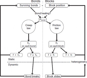
The steps describing how the development of the instability is modeled are shown in Figure 8. As explained above, two phases have to be distinguished:

1. A quasi-static (quiescent) phase corresponding to the nucleation of block sliding and bond rupture.

2. A dynamical (active) phase corresponding to the sliding phase of the blocks and the failure of the bonds.

Fig. 8.

Flow-chart of the modified spring–block model.

3.2. Geometric parameters

We first have to consider the geometric input parameters for modeling the Altelsgletscher. The glacier is discretized into a system of regular cubic blocks. The application of this model to the time evolution of an unstable glacier implies that snow accumulation at the surface of the glacier is neglected, corresponding to a timescale of 1–2 years. This assumption seems to be justified for Altelsgletscher, as its northwestern face has a steep slope (35–40°) and is subjected to strong winds, drifting snow away. In addition, typical snow and ice accumulation rates are low compared with the overall thickness (∼30 m) of the glacier.

In order to obtain a realistic description of the damage and fragmentation process that may develop in the ice mass, we need a sufficient number of blocks. As a compromise between reasonable sampling and numerical speed, we use a model composed of 70 × 70 blocks for this example. It is possible to evaluate the size of the unstable part from analysis of Figure 4 and from direct observations. Accordingly, the glacier surface area was chosen to be ∼4 km², with a mean ice depth of 30 m. As we consider a model composed of 70 × 70 blocks, each block corresponds to a discrete mesh 30 m thick, 30 m long and 30 m wide. The weight of each block is ∼24.75 × 10⁶ kg (density 917 kgm⁻³).

The slope of the bedrock, 𝜙, ranges from 35° (lower part) to 40° (upper part) (Fig. 9). To account for the curvature of the bedrock slope, we used a digital elevation model (DEM) supporting the blocks described above (Fig. 10).

Fig. 9.

Distribution of the slope of the bedrock at the position of the blocks.

Fig. 10.

DEM of the Altels.

We now describe the two key processes in the model, the friction and damage laws, applied to blocks and bonds, respectively.

3.3. Friction law between the discrete blocks and the basal surface

Figure 3 and the discussion in section 2.2 suggest that the central part of the glacier was temperate at the time of its destabilization. The rupture developed and propagated within the ice (on the margin) as well as above the bedrock (central part). These two zones need to be considered here, depending on where the modeled discrete ice blocks lie (either on ice or on the bedrock). The friction law between the discrete blocks and the basal surface should also capture both cases, ice/ice friction and ice/bedrock friction. Guided by the rate and state friction character of rock (Reference DieterichDieterich, 1994) and ice (Reference Fortt and SchulsonFortt and Schulson, 2009; Reference Lishman, Sammonds and FelthamLishman and others, 2011), a rate- and state-dependent friction law seems to be adequate to describe both ice/ice friction and ice/bedrock friction. The version of the rate/state-variable constitutive law, currently most accepted as being in reasonable agreement with experimental data on solid friction, is known as the Dieterich–Ruina law (Reference DieterichDieterich, 1994):

(1)

where the state variable, θ, is usually interpreted as proportional to the surface of contact between asperities of the two surfaces. The constant μ ₀ is the friction coefficient for a sliding velocity and a state variable θ ₀. A and B are coefficients that depend on material properties.

The time evolution of the state variable, θ, is described by

(2)

where D _c is a characteristic slip distance, usually interpreted as the typical size of asperities. The friction law, Equation (1), with Equation (2), accounts for the fundamental properties of a broad range of surfaces in contact, namely that they strengthen (age) logarithmically when ageing at rest, and tend to weaken (rejuvenate) when sliding.

The primary parameter that determines stability, A - B, is a material property. Physically, A- B indicates the sensitivity of the friction coefficient to velocity change: a negative value indicates velocity-weakening leading to an unstable slip; a positive value indicates velocity-strengthening leading to a stable slip. Reference Faillettaz, Sornette and FunkFaillettaz and others (2010) showed that the case A = B is of special interest because it retrieves the main qualitative features of the two classes, and also because, empirically, A is very close to B. Assuming A = B is therefore reasonable and ensures more robust results. The critical time, t _f, signaling the transition from subcritical sliding to dynamical inertial sliding is given in this case (Reference Faillettaz, Sornette and FunkFaillettaz and others, 2010) by

(3)

for μ > μ ₀. (Details of how this equation is obtained are given in the Appendix.) Note that t _f → ∞ for μ ≤ μ ₀, where t _f is the time when the block starts sliding, μ ₀ is a constant friction coefficient, A is a constant parameter depending on material properties and θ ₀ is the state parameter at steady state. The parameter μ is evaluated for each block with the definition of the solid friction, μ = T/N, where T is the tangential force determined from the positions of its connected neighbors and N is the normal component of the weight of the block. The state parameter, θ ₀ in Equation (3), is given by (see Appendix)

(4)

where is generally interpreted as the initial low velocity of a sliding mass, before it starts to accelerate towards its dynamical instability and where D _c can be interpreted as a characteristic slip distance over which different asperities come in contact.

Three parameters have to be correctly evaluated to model the frictional processes within the glacier: μ ₀, A and θ ₀. An increasing friction coefficient with increasing sliding velocity (velocity-strengthening) at low velocities has been observed for polished ice-on-ice (Reference Kennedy, Schulson and JonesKennedy and others, 2000; Reference Montagnat and SchulsonMontagnat and Schulson, 2003), ice-on-granite (Reference Barnes, Tabor and WalkerBarnes and others, 1971) and ice-on-ice along a Coulombic fault (Reference Fortt and SchulsonFortt and Schulson, 2009). A decreasing friction coefficient with increasing sliding velocity (velocity-weakening) at high velocities has also been observed (Reference Barnes, Tabor and WalkerBarnes and others, 1971; Reference Kennedy, Schulson and JonesKennedy and others, 2000). The transition between these two regimes occurs at a velocity of 10⁻⁵ m s⁻¹ (Reference Fortt and SchulsonFortt and Schulson, 2009). These two different behaviors are generally explained by two physical mechanisms, depending on the sliding velocity regimes:

By analogy with rock physics, a rate- and state-dependent friction model for fresh and sea ice was proposed recently (Reference Fortt and SchulsonFortt and Schulson, 2009; Reference Lishman, Sammonds and FelthamLishman and others, 2011). Such a model enables us to explain the change in the friction coefficient when varying sliding velocity along Coulombic shear faults or slip histories. The experiments performed by Reference Fortt and SchulsonFortt and Schulson (2009) at −10°C on sliding along Coulombic shear faults in ice suggest that the ice/ice friction coefficient is velocity-dependent and varies between 0.6 and 1.4, depending on the applied sliding velocity along the fault. As these last results are the closest to our case, we used a mean value of in our calculation.

Once the block slides, the dynamics is controlled by a kinetic friction coefficient, which is in general smaller than the static coefficient, . At low temperatures, Reference Kennedy, Schulson and JonesKennedy and others (2000) and Reference Fortt and SchulsonFortt and Schulson (2009) found a relatively constant friction coefficient around 0.6 for sliding velocities less than 10⁻⁴ m s⁻¹, and rapidly decreasing values down to 0.1 at velocities more than 10⁻⁴ m s⁻¹. As velocities more than 10⁻⁴ m s⁻¹ are not expected in our model describing the nucleation phase of the catastrophic rupture, we assume a kinetic friction coefficient, μ _d = 0.6.

Next, we turn to the evaluation of coefficient A (and B, since we have made the simplifying assumption that B = A) in the rate- and state-dependent friction law (Equation (1)). Laboratory experiments suggest that A is smaller than μ ₀ by typically one and sometimes up to two orders of magnitude for rock (Reference ScholzScholz, 1998, Reference Scholz2002; Reference Ohmura and KawamuraOhmura and Kawamura, 2007), ranging from 0.01 to 0.2. A recent experiment on saline ice suggests that A could be significantly higher for ice (A ≈ 0.3; Reference Lishman, Sammonds and FelthamLishman and others, 2011). As we do not have access to strong experimental constraints and since the friction law should be valid for both ice/ice and ice/bedrock friction, we choose A ≈ 0.1, corresponding to one-tenth of the static friction coefficient, which is the upper limit given by Reference Ohmura and KawamuraOhmura and Kawamura (2007) for rock. This choice seems reasonable for both cases.

The last parameter to be determined is θ ₀ in Equation (4). In the case of a glacier, the sliding velocity is typically of the order of centimeters per day. Therefore a roughly correct estimate is . D _c can be interpreted as a characteristic slip distance over which different asperities come in contact. It is difficult to decide this value. Recent seismological literature reports that D _c lies in the range of tens of centimeters to meters for earthquakes (Reference Mikumo, Olsen, Fukuyama and YagiMikumo and others, 2003; Reference Zhang, Iwata, Irikura, Sekiguchi and BouchonZhang and others, 2003). We arbitrarily choose D _c ≃ 1 m. Inserting this value in Equation (4), we obtain θ ₀ = 100 days.

To account for the heterogeneity and roughness of the sliding surface, the state variable θ _i is reset to a new random value once the dynamical sliding stops. This random value should not be chosen too low, so a block which just stopped sliding does not switch immediately into a new dynamical phase (i.e. t _f = 0). Thus, we assign θ _i = νθ ₀, with ν uniformly distributed between 0.5 and 1.5.

Finally, the possible water lubrication of the bedrock leading to a progressive decrease of the ice/rock frictional resistance is modeled using a progressive decrease of the friction coefficient, μ ₀, at the interface between the simulated ice block and the basal surface. In this way, we account for the progressive onset of the temperate central zone by changing only one parameter.

3.4. Creep law

As discussed in section 3.1, bonds are modeled as linear springs in parallel with an Eyring dashpot. The springs transmit the forces associated with the relative displacements of the blocks. The spring stiffness has also to be evaluated in order to reflect the elastic property of the bulk ice mass. In continuous elasticity, Hooke’s law of elasticity relates stress, σ, and strain, ϵ, via Young’s modulus, E: σ = Eϵ. This leads to the expression: σ _bulk = E _ice(δL/L). This stress is applied to a side surface of the block, S = HL (where H is the height and L the length of the surface), leading to an equivalent force in the bulk, F _bulk = E _ice(δL/L)S. A linear spring is subjected to forces given by F _bond = K _bond δL. In order to find an equivalent behavior, these two forces have to be of the same order, leading to a spring stiffness given by K _bond = E _ice H. Usually values for E _ice are reported to be 9 GPa (Reference Petrenko and WhitworthPetrenko and Whitworth, 1999; Reference PetrovichPetrovich, 2003). However, there is a disagreement of an order of magnitude between measurements of E in the laboratory (9 GPa) and field observations (∼1 GPa), as argued by Reference VaughanVaughan (1995).

Depending on the applied stress, ice has either linear viscous or nonlinear viscous behavior. In glaciers, ice creep is usually described by a nonlinear viscous rheology, called Glen’s flow law (Reference HutterHutter, 1983, and references therein). This law relates strain rate and stress in the secondary creep regime under steady-state conditions. It is thus not possible to use this law to describe tertiary creep and the rupture of a bond. However, Reference HutterHutter (1983) states that the so-called Prandtl–Eyring flow model shows behavior compatible with Glen’s flow law at low stresses. Nonlinear viscous behavior is introduced in our model with an Eyring dashpot in parallel with a linear spring of stiffness, K _bond (which is analogous to the Prandtl–Eyring flow model), following Reference Nechad, Helmstetter, El Guerjouma and SornetteNechad and others (2005). Its deformation, e, is governed by the Eyring dashpot dynamics:

(5)

where the stress in the dashpot, s _dashpot, is given by

(6)

Here s is the total stress applied to the bond and P(e) is the damage accumulated within the bond during its history leading to a cumulative deformation, e. P(e) can be equivalently interpreted as the fraction of representative elements within the bond which have broken, so the applied stress, s, is supported by the fraction, 1 − P(e), of unbroken elements. Following Reference Nechad, Helmstetter, El Guerjouma and SornetteNechad and others (2005), we postulate the following dependence of the damage, P(e), on the deformation, e:

(7)

where e ₀₁ , e ₀₂ and ξ are constitutive properties of the bond material.

Finally, by combining the previous equations, Reference Faillettaz, Sornette and FunkFaillettaz and others (2010) found a creep model that computes the critical time (i.e. failure of the bond) as a function of the stress experienced by the bond, s, given by:

(8)

where

(9)

and

(10)

Creep properties are defined by the parameters K, β, e ₀₁, e ₀₂ and ξ, that we need to fix for our simulations.

We need to find the most appropriate parameters to describe the creep behavior of ice. The ice of natural glaciers has a complex polycrystalline structure composed of crystals of different sizes. From Equation (7), a fraction, 1 – (e ₀₁/e ₀₂) ^ξ , of all the representative elements present undergo abruptfailure immediately after the stress is applied. Since ice does not show significant damage immediately after being loaded, a reasonable assumption is e ₀₁ = e ₀₂. The relative heterogeneity of the material is introduced with the parameter ξ. Despite its complex structure, ice is a fairly homogeneous material compared to a fiber matrix composite. The more homogeneous a material, the greater ξ. In the following, we set ξ = 10 which means that ice is not very heterogeneous; e.g. Reference Nechad, Helmstetter, El Guerjouma and SornetteNechad and others (2005) used ξ ≈ 2 for a fiber matrix composite. Moreover, as e ₀₁ = e ₀₂, it is ξ that influences parameter s ^⋆, i.e. the critical stress above which damage starts. The change in s ^⋆ values is small compared with that of ξ (e.g. ξ = 2 =>. s ^⋆ = 7.5 × 10⁻⁴ E, ξ = 5 => s^* = 2.4 × 10⁻⁴ E, ξ = 10 =>. s ^⋆ = 1.4 × 10⁻⁴ E).

The other parameters describing the deformation of the Eyring dashpot under an applied stress are β for the nonlinear term and K for the linear term. It is difficult to infer such parameters for ice. Reference Nechad, Helmstetter, El Guerjouma and SornetteNechad and others (2005) used β = 50 × 10⁻⁹ Pa⁻¹ and K = 10⁵ s⁻¹ for a fiber matrix composite. As ice is significantly weaker, we arbitrarily choose β = 10⁻⁷ Pa⁻¹ and K = 10⁻³ s⁻¹. With a tensile strength of ice of 1 MPa, we obtain, from Equation (5), de/dt = 10⁻⁴ s⁻¹, which is coherent with the behavior of polycrystalline ice (Reference Schulson and DuvalSchulson and Duval, 2009).

4.1. Description of the simulation

Blocks are distributed in a regular mesh on the inclined plane, so bonds are initially stress-free. At each time-step we evaluate, for each block, the local bed slope from the DEM of the Altels area (Fig. 10). This aims to mimic the real topography of Altelsgletscher. To determine the causes of the glacier collapse, we test the different contributions described by Reference Röthlisberger and KasserRöthlisberger (1981) (section 2.2).

Table 1 summarizes the parameters used in our simulations.

Table 1.

Parameters used for the simulation. n is the linear dimension of the lattice of blocks, which has a total of n × n blocks

4.2. Qualitative results

Is the 1895 Altels collapse solely due to glacier thickening?

To answer this question, we tested the case of a constant friction coefficient in the presence of a progressive increase of block weight. This means that mass is added at a constant rate on each block. In all the simulations performed, results show that an instability starts from the upper part of the glacier, in contradiction to the observations (Fig. 11). This could be explained by the bedrock topography; the slope is indeed steeper in the upper part, inducing an initial sliding of the upper blocks. Then this instability propagates downwards and the whole glacier collapses.

Fig. 11.

Six snapshots describing the rupture progression and sliding instability in the block lattice with a constant friction coefficient, μ ₀, for all blocks, due to an increase of the weight of the blocks (simulating a positive mass balance). The blocks are presented as points at the nodes of the square lattice. The color of each bond indicates the time remaining to rupture: red (close to rupture) to blue (far from rupture). Bonds in compression are drawn as thick black lines. Bonds without unstable tertiary creep damage are represented as thin black lines. Similar results are obtained by progressively decreasing the friction coefficient for all blocks

The progressive thickening is therefore not the cause of the 1895 Altels break-off event.

Is the 1895 Altels collapse due to a local decrease in the friction coefficient?

We now show that the most likely scenario to reproduce the geometry of the observed rupture is to progressively modify the basal properties in a restricted zone, corresponding to the likely temperate area at the bedrock (Reference Röthlisberger and KasserRöthlisberger, 1981).

In the following, the friction coefficient is decreased at different rates, δμ/δt, on three different surface areas (Fig. 12), corresponding to the assumed temperate bedrock zone. This simulates water penetrating the glacier and lubricating the ice/bedrock interface.

Fig. 12.

Zones where the basal friction coefficient is decreased. Their extension was determined according to Reference Röthlisberger and KasserRöthlisberger (1981) (see Fig. 5).

Figure 13 shows the evolution of the set of blocks in the regime where the instability develops. Different phases can be distinguished during this simulation:

Fig. 13.

Six snapshots showing the rupture progression and sliding instability in the block lattice for the largest zone where the basal friction coefficient was progressively reduced. The blocks are presented as points at the nodes of the square lattice. The color of each bond encodes the time remaining to rupture: red (close to rupture) to blue (far from rupture). Bonds in compression are drawn as thick black lines. Bonds without unstable tertiary creep damage are represented as thin black lines.

In the following, the value of μ ₀ is set larger than arctan(max(𝜙)), where 𝜙 is the slope evaluated from the DEM of the glacier bed. In this way, the glacier is assumed to be stable when the simulation starts. At each numerical time-step, the friction coefficient, μ ₀, is decreased by δμ/δt.

1. 1. Initially, blocks situated in the zone where the friction coefficient is decreased start sliding where the bedrock slope is largest. Sliding of these blocks leads to a change in stress experienced by the bonds. This internal bond deformation propagates upstream (Fig. 13a).

2. 2. Then the glacier starts accommodating its new stress state, resulting in a quiet phase. The number of sliding blocks progressively increases, leading to stronger interactions and to synchronization of the sliding blocks (Fig. 13d and e).

3. 3. After a certain time (depending on δμ/δt) the lattice starts fracturing. A large crack appears perpendicular to the main slope around the middle of the lattice (Fig. 13b and c). This corresponds to the opening of the crevasse just below the bergschrund (Fig. 4b).

4. 4. The final instability develops. The blocks located below the upper crevasse start to accelerate and a fracture of side bonds propagates in the bedrock slope direction, forming an unstable slab, which finally slides off (Fig. 13f).

Initiation of the instability

For each of the three process zones (i.e. the area where the friction coefficient is decreased) and for different rates of decrease of the friction coefficient (RDFCs), δ(μ)/δ(t), we show the number of sliding blocks at each time-step in Figure 14. It appears that, in all cases, the instability evolves rapidly, typically within 1–2 days. Two different regimes can be distinguished: a first quiescent one, in which isolated blocks slide, and a second active one, in which blocks start to slide in clusters, leading to the final collapse.

Fig. 14.

Fraction of sliding blocks within the glacier for different δμ/δt as a function of time, for the three different process zones (minimum, medium and maximum corresponding to Figure 12a, b and c, respectively).

The number of sliding blocks after the onset of the instability depends on the RDFC. The greater the RDFC, the larger the number of sliding blocks. When the RDFC is small, the glacier has time to adapt to changes in basal conditions. In this case, the size of the initial unstable cluster is strictly given by the size of the process zone.

Damage evolution within the glacier

In order to measure the damage evolution within the glacier, we count the number of surviving bonds during each simulation. Figure 15 shows the number of surviving bonds within the lattice at each time-step for different process zones and different RDFCs. A rapid increase in the damage a few days after the initiation of the instability can be observed for all simulations. Moreover, this increase does not seem to depend on the RDFC. Results show that, once the behavior enters the active regime, bonds start to fail, leading to the opening of the crown crevasse. That the crevasse opens very rapidly, typically within a few days, was observed by Reference HeimHeim (1895).

Fig. 15.

Fraction of the surviving bonds within the glacier for different RDFCs, δμ/δt, as a function of time, for the three different process zones (minimum, medium and maximum corresponding to Figure. 12a, b and c, respectively).

Energy analysis

In order to detect precursors to the rupture, we investigated the evolution of the energy stored in the bonds, the kinetic energy (corresponding to the flow velocity) and the radiated energy (i.e. energy released by the rupture of bonds) during the destabilization process (Fig. 16).

Fig. 16.

Evolution of the energy stored in the bonds, E _b, of the kinetic energy, E _k, and of the radiated energy, δE _r, during the destabilization process.

Six phases can be distinguished. (1) The glacier remains in a stable phase. (2) Initiation of the instability. (3) The number of sliding blocks drastically increases. (4) The number of sliding blocks reaches a maximum and the energy stored in the bonds increases. Note that the increase of kinetic and radiated energies starts to be visible. (5) The energy stored in the bonds drops because the crown crevasse opens. The number of sliding blocks remains unchanged and the instability is now established. Both the kinetic and radiated energies increase. (6) After an increase of the energy stored in the bonds, clusters of bonds fail.

These results show that no precursor to the instability can be inferred from the time evolution for the energies considered earlier than a few days before the break-off.

4.3. Quantitative results

The results obtained with the spring–block model are summarized in the following.

Occurrence of the instability as a function of δ(μ)/δ(t) To assess whether the RDFC, δ(μ)/δ(t)), influences the final time of rupture, we performed independent runs with different rates and evaluated their respective rupture times. The results show that the rupture occurs earlier for greater RDFC, which is not surprising (Fig. 17). However, the time of rupture does not depend linearly on RDFC but follows a power law with an exponent, b, of −0.82. The exponent was estimated using the maximum-likelihood fitting method with goodness-of-fit tests based on the Smirnov test (e.g. Reference Clauset, Shalizi and NewmanClauset and others, 2009). This means that for small RDFC the glacier has time to adapt to these changes and the final instability arises later than in the case of large RDFC.

Fig. 17.

Time of rupture, t _i, as a function of the RDFC, δμ/δt, for the medium process zone. The dotted line plots the equation: t _i ∼ (δμ/δt)^−0.82.

The influence of the surface area of the process zone, S, on the time of rupture, t _i, was tested and we found an inverse effect compared with the RDFC. Specifically, a glacier for which a large RDFC acts on a small process zone becomes unstable after the same time as a glacier subjected to a small RDFC applied to a large process zone. This can be summarized by plotting the reduced variable t _i S ^0.78 as a function of (δμ/δt)^−0.82, as shown in Figure 18.

Fig. 18.

Time of rupture, t _i, as a function of δμ/δt. The dotted line plots the equation: t _i S ^0.78 ∼ 116(δμ/δt)^−0.82.

The determination of these two parameters is not yet possible, especially for the area of the process zone. The collapse of three power laws shown in Figure 18 can be rewritten as t _i ∼ [S(δμ/δt)] ^−ν , where ν ≈ 0.8. This law expresses a combined ‘size’ effect (through the term S) and a rate-dependence effect (through the term δμ/δt). Similar behavior is found in most heterogeneous mechanical systems going to failure (Reference CollinsCollins, 1993; Reference CarpinteriCarpinteri, 1996). Interestingly, the combined dependence of the failure time, t _i, on the unstable area, S, and on the rate, δμ/δt, is through their product, suggesting that the driving mechanism for the failure time is the total shear force applied to the unstable area.