2.1 Setup

The following notations are used throughout the article. We use lowercase letters x, boldface lowercase letters $\boldsymbol {v}$ , and boldface capital letters $\boldsymbol {X}$ to represent scalars, vectors, and matrices, respectively. 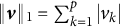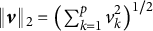Additionally, for any vector $\boldsymbol {v}^T = (v_1 , \ldots , v_p)$ , $\Vert \boldsymbol {v} \Vert _1 = \sum _{k=1}^p |v_k| $ denotes the $\ell _1$ vector norm and $\Vert \boldsymbol {v} \Vert _2 = \left ( \sum _{k=1}^p v_k^2 \right )^{1/2}$ denotes the $\ell _2$ vector norm. For any matrix $\boldsymbol {A} = (a_{kl})$ , $\Vert \boldsymbol {A} \Vert _{1,1} = \Vert \mathrm {vec}(\boldsymbol {A}) \Vert _{1} = \sum _{k}\sum _{l} | a_{kl}|$ denotes the element-wise $\ell _1$ vector norm of the matrix, $\Vert \boldsymbol {A} \Vert _{\infty ,\infty } = \max _{k,l} | a_{kl}|$ denotes the element-wise $\ell _\infty $ vector norm of the matrix, and $\Vert \boldsymbol {A} \Vert _F = \Vert \mathrm {vec}(\boldsymbol {A}) \Vert _{2} = \left ( \sum _{k}\sum _{l} a_{kl}^2 \right )^{1/2}$ denotes the Frobenius norm, which corresponds to the $\ell _2$ norm of the vectorized matrix.

Let $\boldsymbol {X}$ be an $n \times p$ matrix of data that contains n realizations of p variables. We denote the corresponding sample correlation matrix as $\boldsymbol {R}$ . The singular value decomposition of the correlation matrix, respectively, called eigendecomposition, can be written as follows:

$$ \begin{align*} \boldsymbol{R} = \boldsymbol{V} \boldsymbol{L} \boldsymbol{V}^T, \; \boldsymbol{V}^T \boldsymbol{V} = \boldsymbol{I}_p, \; l_1 \geq \cdots \geq l_p \geq 0 , \end{align*} $$

where $\boldsymbol {L}$ contains the eigenvalues (singular values) of $\boldsymbol {R}$ on the diagonal, and $\boldsymbol {V} = (\boldsymbol {v}_1,\ldots ,\boldsymbol {v}_p)$ are the eigenvectors (singular vectors).

As will be discussed below, our goal is to identify two distinct submatrices $\boldsymbol {X}_j$ ( $n \times p_{j}$ ) and $\boldsymbol {X}_{j'}$ ( $n \times p_{j'}$ ) of $\boldsymbol {X}$ , with $p =p_{j} + p_{j'}$ , which exhibit the smallest average correlation between them for the purpose of computing Revelle’s beta. $\boldsymbol {X}_j$ and $\boldsymbol {X}_{j'}$ can be considered as clusters that identify $p_j$ and $p_{j'}$ many variables.

Although the exact submatrices are currently unknown, we can still assume the convenient order $\boldsymbol {X} = (\boldsymbol {X}_{j},\boldsymbol {X}_{j'})$ 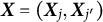without loss of generality, since any such ordering can be obtained using column permutation. The sample correlation matrix can thus be written as

(1) $$ \begin{align} \boldsymbol{R} = \begin{pmatrix} \boldsymbol{R}_j & \boldsymbol{R}_{jj'} \\ \boldsymbol{R}_{jj'}^T & \boldsymbol{R}_{j'} \end{pmatrix} , \end{align} $$

where $\boldsymbol {R}_j$ ( $p_j \times p_j$ ) is the correlation matrix of $\boldsymbol {X}_{j}$ , $\boldsymbol {R}_{j'}$ ( $p_{j'} \times p_{j'}$ ) is the correlation matrix of $\boldsymbol {X}_{j'}$ , and $\boldsymbol {R}_{jj'}$ ( $p_{j} \times p_{j'}$ ) contains the correlations between these two submatrices, that is, the between-test correlations.

Revelle (Reference Revelle1979) proposed a reliability measure based on the worst split-half of a test, commonly known as Revelle’s beta. For a split of $\boldsymbol {X}$ into the two halves $\boldsymbol {X}_j$ and $\boldsymbol {X}_{j'}$ , this split-half reliability estimate is defined as the average between-half correlations $\Vert \boldsymbol {R}_{jj'} \Vert _{1,1} / (p_j p_{j'})$ times the total number of items squared $p^2$ , and scaled by the total correlation $\Vert \boldsymbol {R} \Vert _{1,1}$ . Thus, the coefficient can be written as

(2) $$ \begin{align} \frac{ p^2 \Vert \boldsymbol{R}_{jj'} \Vert_{1,1} / (p_j p_{j'}) }{ \Vert \boldsymbol{R} \Vert_{1,1} } = \frac{\Vert \boldsymbol{R}_{jj'} \Vert_{1,1} / (p_j p_{j'}) }{\Vert \boldsymbol{R} \Vert_{1,1} / p^2} . \end{align} $$

Consequently, this estimate scales the average of absolute components of $\boldsymbol {R}_{jj'}$ by the average of absolute components of $\boldsymbol {R}$ , yielding a value between zero and one.

Although split-half reliability can also be formulated in terms of the covariance matrix, the present manuscript focuses on correlation matrices and therefore on standardized tests. This focus stems from an assumption in Bauer (Reference Bauer2025b), whose methodology underlies the proposed computation of Revelle’s beta. In particular, the assumption ensures that individual items remain distinguishable. A brief overview of the methodology is provided later.

This restriction should be kept in mind when interpreting the coefficient. Since the use of correlations removes differences in item variances, the resulting value is Revelle’s beta for the standardized item scores, rather than necessarily for a raw-score total. This distinction is expected to be minor when items are measured on the same response scale and have similar variances, but it may matter when items have different response formats, substantially different variances, or are intentionally weighted differently. In such cases, standardization may affect both the value of beta and the split identified as the worst split-half.

2.2 Computation of the worst split-half reliability

In practice, when $\boldsymbol {X}_j$ and $\boldsymbol {X}_{j'}$ are unknown, for example, when they represent underlying latent factors, we aim to find these by minimizing Equation (2). This minimum is the worst split-half reliability, known as Revelle’s beta. Consequently, to identify the disjoint submatrices $\boldsymbol {X}_j$ and $\boldsymbol {X}_{j'}$ , we solve the following optimization problem:

(3) $$ \begin{align} \beta = \min\limits_{\boldsymbol{X}_j,\boldsymbol{X}_{j'}} \frac{\Vert \boldsymbol{R}_{jj'} \Vert_{1,1} / (p_j p_{j'}) }{\Vert \boldsymbol{R} \Vert_{1,1} / p^2} . \end{align} $$

We note that identifying the submatrices with the worst split-half reliability is conceptually identical to identifying the submatrices with the lowest average absolute between-test correlations.

Remark 2.1. The arguments $\boldsymbol {X}_j$ and $\boldsymbol {X}_{j'}$ that minimize the optimization problem in (3) are identical to the ones of the optimization problem

$$ \begin{align*} \min\limits_{\boldsymbol{X}_j,\boldsymbol{X}_{j'}} \frac{\Vert \boldsymbol{R}_{jj'} \Vert_{1,1} }{ p_{j} p_{j'} } . \end{align*} $$

This optimization problem is known as average linkage clustering in clustering contexts, and computation of Revelle’s beta is therefore conceptually identical to a divisive (“top-down”) clustering task: we iteratively split $\boldsymbol {X}$ into subsequently smaller subtests using average linkage, until each variable is contained in a single subtest. Consequently, we start by splitting $\boldsymbol {X}$ into $\boldsymbol {X}_j$ and $\boldsymbol {X}_{j'}$ , then splitting $\boldsymbol {X}_j$ as well as $\boldsymbol {X}_{j'}$ , and so on.

However, a drawback of divisive clustering is its computational cost: when splitting p variables, there are $2^{p-1}-1$ candidate combinations which cannot all be checked for large p. In the context of clustering, however, a recent approach reduces this exponential problem to a quadratic one. The idea is to find the best block-diagonal approximation of the correlation matrix from a set of block-diagonal matrices comprising two blocks, with respect to some function $f:\mathbb {R}^{p\times p} \to \mathbb {R}$ 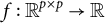via

(4) $$ \begin{align} \min\limits_{\boldsymbol{X}_j,\boldsymbol{X}_{j'}} f\left( \begin{pmatrix} \boldsymbol{R}_j & \boldsymbol{R}_{jj'} \\ \boldsymbol{R}_{jj'}^T & \boldsymbol{R}_{j'} \end{pmatrix} - \begin{pmatrix} \boldsymbol{R}_j & \boldsymbol{0} \\ \boldsymbol{0} & \boldsymbol{R}_{j'} \end{pmatrix} \right) . \end{align} $$

For clustering using average linkage, this corresponds to the optimization problem in Equation (4) with $f(\boldsymbol {A}) \mapsto \Vert \boldsymbol {A} \Vert _{1,1}/(2p_j p_{j'})$ given as

$$ \begin{align*}\min\limits_{\boldsymbol{X}_j,\boldsymbol{X}_{j'}} \frac{1}{2p_{j} p_{j'}} \Vert \begin{pmatrix} \boldsymbol{R}_j & \boldsymbol{R}_{jj'} \\ \boldsymbol{R}_{jj'}^T & \boldsymbol{R}_{j'} \end{pmatrix} - \begin{pmatrix} \boldsymbol{R}_j & \boldsymbol{0} \\ \boldsymbol{0} & \boldsymbol{R}_{j'} \end{pmatrix} \Vert_{1,1} , \end{align*} $$

or, equivalently,

$$ \begin{align*}\min\limits_{\boldsymbol{X}_j,\boldsymbol{X}_{j'}} \frac{1}{p_{j} p_{j'}} \Vert \boldsymbol{R}_{jj'} \Vert_{1,1} , \end{align*} $$

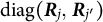
where the approximation is with respect to the average absolute matrix components of $\boldsymbol {R}_{jj'}$ . Bauer (Reference Bauer2025b, Reference Bauer2025c) demonstrated that sparse eigenvectors of the correlation matrix, which are sparse approximations of the eigenvectors $\boldsymbol {V}$ that contain many zeros, identify the correlation matrix $\boldsymbol {R}_{jj'}$ that minimizes the split-half in (3). Specifically, the sparse eigenvectors mirror the block diagonal matrix approximation $\mathrm {diag}(\boldsymbol {R}_{j},\, \boldsymbol {R}_{j'})$ of the correlation matrix $\boldsymbol {R}$ in (1), thereby identifying $\boldsymbol {X}_j$ and $\boldsymbol {X}_{j'}$ .

We now give a recap of this method, named hierarchical clustering using singular vectors (HC-SVD), and refer to Bauer (Reference Bauer2025b) for an elaborate introduction to HC-SVD. First, we note that if the correlation matrix $\boldsymbol {R}$ in (1) was a block diagonal matrix, that is, if $\boldsymbol {R}_{jj'} = \boldsymbol {0}$ , then its eigenvectors $\boldsymbol {V}$ exhibit also a block diagonal structure that mirrors this block diagonal shape (Bauer, Reference Bauer2025b; Bauer & Drabant, Reference Bauer and Drabant2021). 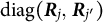If however $\boldsymbol {R}_{jj'} \neq \boldsymbol {0}$ , which is commonly the case in real-world application, the eigenvectors are perturbed and do not mirror the underlying block diagonal structure $\mathrm {diag}(\boldsymbol {R}_{j},\, \boldsymbol {R}_{j'})$ . In HC-SVD, sparse eigenvectors are computed by shrinking these perturbations back toward zero, thereby revealing again the block diagonal structure of the eigenvectors which aligns with the block diagonal structure of the correlation matrix. According to the Eckart–Young theorem (Eckart & Young, Reference Eckart and Young1936), the best rank-one approximation of a symmetric matrix in the Frobenius norm is determined by its first eigenvector and eigenvalue. This can be formulated as

$$ \begin{align*}\min_{l,\, \boldsymbol{v}} \Vert \boldsymbol{R} - l \boldsymbol{v} \boldsymbol{v}^T \Vert_F^2 \;\; \mathrm{subject \; to} \;\; \Vert \boldsymbol{v} \Vert_2^2 = 1 . \end{align*} $$

Building on this, sparse eigenvectors are computed using the following optimization problem (Shen & Huang, Reference Shen and Huang2008):

(5) $$ \begin{align} \min\limits_{\boldsymbol{v}, \tilde{\boldsymbol{v}}} \Vert \boldsymbol{R} - \tilde{\boldsymbol{v}} \boldsymbol{v}^T \Vert_F^2 \;\; \mathrm{subject \; to} \;\; \Vert \boldsymbol{v} \Vert_2^2 = 1, \; \Vert \boldsymbol{v} \Vert_1 \leq c . \end{align} $$

This formulation yields the first sparse eigenvector $\check {\boldsymbol {v}}_1$ with $\Vert \check {\boldsymbol {v}}_1 \Vert _2^2 = 1$ subject to the $\ell _1$ sparsity constraint c. $\tilde {\boldsymbol {v}}$ is allowed to vary and absorbs the corresponding “eigenvalue” $\check {l}_1$ , which means that the optimal $\tilde {\boldsymbol {v}}$ corresponds to the scaled vector $ \check {l}_1 \check {\boldsymbol {v}}_1$ . The remaining sparse eigenvectors $\check {\boldsymbol {v}}_k$ for $k>1$ can be calculated iteratively where the correlation matrix $\boldsymbol {R}$ must be replaced by the residual matrices of the sequential matrix approximations.

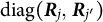
The approach underlying HC-SVD is then computing p sparse eigenvectors, each with $s \in \{1, \ldots , p-1\}$ components shrunk toward zero, to identify $\mathrm {diag}(\boldsymbol {R}_{j},\, \boldsymbol {R}_{j'})$ . This reduces the number of candidate splits to check from $2^{p-1}-1$ to $p(p-1)$ , resulting in a quadratic problem that is computationally feasible even for large p. Checking a reduced subset of candidate splits carries the theoretical risk that the split (argument) minimizing (3) is missed. However, we can establish a regime in which the procedure is guaranteed to identify the minimum. Bauer (Reference Bauer2025b) derived a bound on the off-diagonal block $\boldsymbol {R}_{jj'}$ that ensures the optimal split is perfectly recovered by HC-SVD. For completeness, we restate this recovery guarantee below. However, when only $p(p-1)$ instead of all $2^{p-1}-1$ candidate splits are checked, there is a risk that the split (argument) minimizing Equation (3) is not considered. However, Bauer (Reference Bauer2025b) provides a bound on $\boldsymbol {R}_{jj'}$ that guarantees that the optimal split is recovered by HC-SVD. For completeness, we restate the corresponding result below.

Theorem 2.2 (From Theorem 1 of Bauer, Reference Bauer2025b)

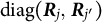
Consider a correlation matrix as in (1). The sparse eigenvector $\check {\boldsymbol {v}}$ with eigenvalue $\check {l}$ computed using the optimization problem in (5) mirrors the block diagonal matrix $\mathrm {diag}(\boldsymbol {R}_{j} ,\, \boldsymbol {R}_{j'})$ if

(6) $$ \begin{align} \frac{1}{p} \Vert \boldsymbol{R}_{jj'} \Vert_{\infty , \infty}\leq \max \{ |\check{\boldsymbol{v}}|_{(p_j)} , |\check{\boldsymbol{v}}|_{(p_{j'})} \}. \end{align} $$

Here, $|\check {\boldsymbol {v}}|_{(p)}$ denotes the p-th largest absolute component of the vector $\check {\boldsymbol {v}}$ .

When this condition holds, the method is guaranteed to identify the true worst split-half partition. Bauer (Reference Bauer2025b) further argues that detection of the block diagonal matrix can be improved by computing the sparse eigenvectors of $\boldsymbol {R}^{\circ h}$ instead of $\boldsymbol {R}$ . Here, $\odot $ denotes the Hadamard (element-wise) product, and $\boldsymbol {R}^{\circ h} = \underbrace { \boldsymbol {R} \odot \cdots \odot \boldsymbol {R} }_{h \text { times}} = (r_{kl}^h)$ 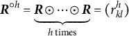defines the Hadamard power of order h. Since $|r_{kl}| \leq 1$ , the intuition is that taking the Hadamard powers shrinks most correlation coefficients toward zero. Importantly, the off-block coefficients in $\boldsymbol {R}_{jj'}$ shrink faster than the within block coefficients in $\boldsymbol {R}_j$ and $\boldsymbol {R}_{j'}$ , because $\Vert \boldsymbol {R}_{jj'}\Vert _{1,1}$ minimizes the between-test correlation. This allows for better detection according of the optimal split, as the bound in (6) from Theorem 2.2 is more likely to be satisfied.

2.3 Visualization of Revelle’s beta

Let us now denote $\beta _j$ as Revelle’s beta of any matrix $\boldsymbol {X}_j$ with correlation matrix $\boldsymbol {R}_j$ , and $\beta $ be the corresponding measure of $\boldsymbol {X}$ as in (3). The result of hierarchical clustering methods is interpretable without inversions via a dendrogram if the resulting distance matrix is ultrametric (Hartigan, Reference Hartigan1967; Johnson, Reference Johnson1967). However, Revelle’s beta satisfies the ultrametric property only under restrictive assumptions.

Theorem 2.3. Consider a correlation matrix as in (1), and let $\boldsymbol {X}_j$ and $\boldsymbol {X}_{j'}$ be the arguments that yield the worst split-half reliability in (3). Revelle’s beta is ultrametric, meaning that $\beta \leq \min \{\beta _{j},\, \beta _{j'}\}$ , if

$$ \begin{align*} \frac{\Vert \boldsymbol{R}_{j} \Vert_{1,1}}{p_{j}^2} \leq \frac{\Vert \boldsymbol{R} \Vert_{1,1}}{p^2} \quad \text{ and } \quad \frac{\Vert \boldsymbol{R}_{j'} \Vert_{1,1}}{p_{j'}^2} \leq \frac{\Vert \boldsymbol{R} \Vert_{1,1}}{p^2} . \end{align*} $$

Consequently, if the average absolute correlation coefficients of $\boldsymbol {X}$ are larger than the average absolute correlation coefficients within its two subtests, Revelle’s beta is ultrametric. However, since $\boldsymbol {R}$ includes the submatrix $\boldsymbol {R}_{jj'}$ , which contains the correlations between the two subtests $\boldsymbol {X}j$ and $\boldsymbol {X}{j'}$ , these conditions are not necessarily satisfied in practice.

In contrast, HC-SVD using average linkage produces an ultrametric distance matrix (Bauer, Reference Bauer2025b). As discussed above, the worst-split half aligns with the splits identified by HC-SVD using average linkage. Consequently, all splits according to Revelle’s beta can be hierarchically visualized using a dendrogram, where the heights of this dendrogram are computed via average linkage. While the heights of this dendrogram do not correspond to the actual values of Revelle’s beta, its hierarchical structure is identical to that implied by Revelle’s beta and thus accurately represents all splits.

2.4 Comments on ICLUST

Revelle (Reference Revelle1978) introduced the item cluster analysis (ICLUST) procedure to identify subtests exhibiting the worst split-half reliabilities. This “bottom-up” approach iteratively merges subtests using agglomerative clustering with complete linkage to form candidate clusters. A candidate cluster $\boldsymbol {X} = (\boldsymbol {X}_j,\, \boldsymbol {X}_{j'})$ 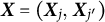is constructed by merging $\boldsymbol {X}_j$ and $\boldsymbol {X}_{j'}$ if two internal consistency criteria are satisfied. Specifically, the merged cluster $\boldsymbol {X}$ must yield a higher Cronbach’s alpha than either subtest ( $\alpha> \min \{\alpha _j,\, \alpha _{j'}\}$ ), and a higher Revelle’s beta than the average of the corresponding betas ( $\beta> (\beta _j + \beta _{j'})/2$ ).

Nowadays, alternative combinations of these internal consistency tests are also considered. For Cronbach’s alpha, the conditions may take one of the forms

$$ \begin{align*}\alpha> \min\{\alpha_{j},\, \alpha_{j'}\} \,, \,\,\, \alpha > (\alpha_{j} + \alpha_{j'})/2 \,, \text{ or } \alpha > \max\{\alpha_{j},\, \alpha_{j'}\} ,\end{align*} $$

and analogously for Revelle’s beta,

$$ \begin{align*}\beta> \min\{ \beta_{j},\, \beta_{j'}\} \,, \,\,\, \beta > ( \beta_{j} + \beta_{j'})/2 \,, \text{ or } \beta > \max\{ \beta_{j},\, \beta_{j'}\} .\end{align*} $$

Implementations of these consistency tests are discussed in Section 3 and in the corresponding part of the Supplementary Material.

Among these, the conditions $\alpha> \min \{\alpha _{j},\, \alpha _{j'}\}$ and $\beta> \min \{\beta _{j},\, \beta _{j'}\}$ are the most relaxed, as they are satisfied whenever any of the other conditions hold. Consequently, if these relaxed conditions are not met, none of the stricter ones will hold either. However, these conditions align with Revelle’s beta only under restrictive assumptions, as can be concluded from the following theorem.

Theorem 2.4. Consider a correlation matrix as in (1), and let $\boldsymbol {X}_j$ and $\boldsymbol {X}_{j'}$ be the arguments that yield the worst split-half reliability in (3). The condition $\alpha> \min \{\alpha _{j},\, \alpha _{j'}\}$ is satisfied if

(7) $$ \begin{align} \frac{\Vert \boldsymbol{R}_{j} \Vert_{1,1}}{p_{j}} \geq \frac{\Vert \boldsymbol{R} \Vert_{1,1}}{p} \quad \text{ and } \quad \frac{\Vert \boldsymbol{R}_{j'} \Vert_{1,1}}{p_{j'}} \geq \frac{\Vert \boldsymbol{R} \Vert_{1,1}}{p}. \end{align} $$

Using the identity $\Vert \cdot \Vert _{1,1} = \Vert \cdot \Vert _{1,1}^{1/2} \Vert \cdot \Vert _{1,1}^{1/2} $ , the left condition in Equation (7) can be rewritten as

(8) $$ \begin{align} \left( \frac{\Vert \boldsymbol{R}_{j} \Vert_{1,1}}{p_{j}^2} \right)^{1/2} \Vert \boldsymbol{R}_{j} \Vert_{1,1}^{1/2} \geq \left( \frac{\Vert \boldsymbol{R} \Vert_{1,1}}{p^2} \right)^{1/2} \Vert \boldsymbol{R} \Vert_{1,1}^{1/2} . \end{align} $$

The right condition can be rewritten analogously and is omitted here for brevity.

In the context of Theorem 2.3, we argued that $\Vert \boldsymbol {R}_{j} \Vert _{1,1}/p_{j}^2 \geq \Vert \boldsymbol {R} \Vert _{1,1}/p^2 $ , and therefore also $( \Vert \boldsymbol {R}_{j} \Vert _{1,1}/p_{j}^2)^{1/2} \geq ( \Vert \boldsymbol {R} \Vert _{1,1}/p^2 )^{1/2}$ , might generally be valid. However, regarding the remaining terms $\Vert \boldsymbol {R}_{j} \Vert _{1,1}^{1/2} $ and $\Vert \boldsymbol {R}\Vert _{1,1}^{1/2} $ on the left- and right-hand sides of Equation (8), we note that $\Vert \boldsymbol {R} \Vert _{1,1} = \Vert \boldsymbol {R}_{j} \Vert _{1,1} + \Vert \boldsymbol {R}_{j'} \Vert _{1,1} + 2\Vert \boldsymbol {R}_{jj'} \Vert _{1,1}> \Vert \boldsymbol {R}_{j} \Vert _{1,1} $ , which imposes restrictions on the terms in Equation (8) and thus also in (7). Below, we discuss an example in which the ICLUST conditions are not satisfied, meaning that the procedure stops identifying the worst split-half reliability.

To the best of our knowledge, the conditions about Revelle’s beta cannot be simplified further. Nevertheless, the following statement follows directly from Theorem 2.3.

Corollary 2.5. Consider a correlation matrix as in (1), and let $\boldsymbol {X}_j$ and $\boldsymbol {X}_{j'}$ be the arguments that yield the worst split-half reliability in (3). The condition $\beta> \min \{\beta _{j},\, \beta _{j'}\}$ is not satisfied if

$$ \begin{align*} \frac{\Vert \boldsymbol{R}_{j} \Vert_{1,1}}{p_{j}^2} \leq \frac{\Vert \boldsymbol{R} \Vert_{1,1}}{p^2} \quad \text{ and } \quad \frac{\Vert \boldsymbol{R}_{j'} \Vert_{1,1}}{p_{j'}^2} \leq \frac{\Vert \boldsymbol{R} \Vert_{1,1}}{p^2} . \end{align*} $$

We now consider an example where none of the ICLUST conditions are satisfied, implying that the algorithm fails to identify the worst split-half reliability by construction.

Example 2.6. Consider the correlation matrices $\boldsymbol {R}$ , $\boldsymbol {R}_j$ , and $\boldsymbol {R}_{j'}$ as in (1) with

$$ \begin{align*}\boldsymbol{R} = \begin{pmatrix} 1 & 0.9 & 0.8 && 0.4 & 0.4 & 0.4 \\ 0.9 & 1 & 0.8 && 0.4 & 0.4 & 0.4 \\ 0.8 & 0.8 & 1 && 0.4 & 0.4 & 0.4 \\[0.3cm] 0.4 & 0.4 & 0.4 && 1 & 0.9 & 0.8 \\ 0.4 & 0.4 & 0.4 && 0.9 & 1 & 0.8 \\ 0.4 & 0.4 & 0.4 && 0.8 & 0.8 & 1 \end{pmatrix} \,, \,\, \boldsymbol{R}_j = \boldsymbol{R}_{j'} = \begin{pmatrix} 1 & 0.9 & 0.8 \\ 0.9 & 1 & 0.8 \\ 0.8 & 0.8 & 1 \end{pmatrix}. \end{align*} $$

Then, $\alpha \approx 0.89 \not> \min \{\alpha _j,\, \alpha _{j'}\} \approx 0.94$ and $\beta \approx 0.62 \not> \min \{\beta _j,\, \beta _{j'}\} = 0.9$ , and consequently none of the ICLUST conditions are satisfied and the procedure stops.

Code to replicate this example is available in the Supplementary Material.

2.5 Comments on the computation of Guttman’s lambda four

Guttman (Reference Guttman1945) introduced a series of lower bounds for reliability. Similar to Revelle’s beta, the fourth of these bounds, commonly referred to as Guttman’s lambda four, considers a split of the test into two parts. Although originally defined for an arbitrary split-half, it is nowadays typically interpreted as the greatest split-half reliability (Jackson & Agunwamba, Reference Jackson and Agunwamba1977; Revelle & Zinbarg, Reference Revelle and Zinbarg2009). Thus, as with Revelle’s beta, for a data matrix comprising p items, there are $2^{p-1}-1$ candidate splits.

However, the greatest split-half reliability cannot be computed using the same approach as that used for identifying the worst split-half. To elaborate, Guttman’s lambda four is defined as

(9) $$ \begin{align} \lambda_4 = \max\limits_{\boldsymbol{X}_j,\boldsymbol{X}_{j'}} \frac{4 \Vert \boldsymbol{R}_{jj'}\Vert_{1,1} }{\Vert \boldsymbol{R} \Vert_{1,1}} . \end{align} $$

Similar as for Revelle’s beta, we note that identifying the submatrices with the greatest split-half reliability is conceptually identical to identifying the submatrices that exhibit the largest sum of between-test correlation in absolute terms.

Remark 2.7. The arguments $\boldsymbol {X}_j$ and $\boldsymbol {X}_{j'}$ that minimize the optimization problem in (9) are identical to the ones of the optimization problem

(10) $$ \begin{align} \max\limits_{\boldsymbol{X}_j,\boldsymbol{X}_{j'}} \Vert \boldsymbol{R}_{jj'}\Vert_{1,1} . \end{align} $$

However, this optimization problem does not align with Equation (4) as it corresponds to finding the worst instead of best block diagonal matrix approximation with respect to the function $f(\boldsymbol {A}) \mapsto 2 \Vert \boldsymbol {A} \Vert _{1,1}$ .

Moreover, to the best of our knowledge, it is not possible to transform the optimization problem in Equation (10) into the form of Equation (4). Such a transformation would require mapping large (absolute) values of $\boldsymbol {R}$ to small (absolute) ones, and vice versa, effectively turning a maximization problem into a minimization problem. This transformation would not necessarily preserve positive definiteness, as shown, for example, in Theorem 2.1 of FitzGerald et al. (Reference FitzGerald, Micchelli and Pinkus1995), which is however a requirement for the approach proposed by Bauer (Reference Bauer2025b).

3.1 Preliminaries

All computational results in Section 3 and 4 were conducted in R 4.1.3 (R Core Team, 2022) on a PC running macOS Sequoia 15.6.1. with $8$ GB of RAM. Code to replicate the simulations and examples of these sections alongside details about computational implementations are provided in the Supplementary Material. Furthermore, computing Revelle’s beta using HC-SVD has been implemented specifically for this research project in the R package blox (Bauer, Reference Bauer2025a).

3.2 Methods to compare

We compare our approach to ICLUST, which is implemented in the R package psych (Revelle, Reference Revelle2023). Revelle (Reference Revelle1979) suggested that agglomerative (“bottom-up”) hierarchical clustering using average linkage could be employed to identify the worst split-halves. However, he noted that agglomerative clustering does not always find the true worst split. Bauer (Reference Bauer2025b) elaborates on this argument and showcases the differences between agglomerative and divisive clustering. Nonetheless, given that agglomerative hierarchical clustering with average linkage is a well-established method that exhibits fast computation times, we include it in our simulation study for comparison in the context of identifying Revelle’s beta. Furthermore, an ad-hoc procedure is to consider only a randomly chosen subset of candidate splits. However, such a procedure cannot guarantee to find the worst split-half by construction.

There are also other non-agglomerative clustering methodologies like divisive analysis clustering (DIANA) introduced by Kaufman and Rousseeuw (Reference Kaufman and Rousseeuw1990) or an approach by Bottazzi Schenone et al. (Reference Bottazzi Schenone, Cavicchia, Vichi and Zaccaria2025) and Cavicchia et al. (Reference Cavicchia, Vichi and Zaccaria2020) that aims to identify hierarchical clusters by finding a so-called ultrametric correlation matrix that fits the underlying data. However, their performances are less robust compared to HC-SVD (see Bauer, Reference Bauer2025b for a comparison) and are therefore not considered in this work.

3.3 Simulation designs

We consider two simulation designs to evaluate the performance of the different methods. In both designs, we construct a correlation matrix $\boldsymbol {R}$ from a data matrix $\boldsymbol {X}$ ( $n\times p$ ) of rank k. Specifically, the data matrix is generated as $\boldsymbol {X} = \boldsymbol {U} \boldsymbol {D} \boldsymbol {V}^T + \boldsymbol {E}$ , where $\boldsymbol {U}^T \boldsymbol {U} = \boldsymbol {I}_k$ , $\boldsymbol {V}^T \boldsymbol {V} = \boldsymbol {I}_k$ , $\boldsymbol {D} = \mathrm {diag}(d, \ldots , d)$ ( $k \times k$ ), and $\boldsymbol {E}$ is a noise matrix with components drawn independently from an $N(0, 0.5^2)$ distribution. To ensure orthonormality of $\boldsymbol {U}$ , we generate it as the left orthonormal matrix of a QR decomposition of a matrix with independently $N(0,1)$ components. Across both simulation designs, we set $n = 5p$ . Thus, the matrix $\boldsymbol {E}$ introduces noise to the factor structure, while general sample noise is added by observing n realizations. The two simulation designs A and B differ in how the matrix $\boldsymbol {V}$ is constructed.

1. A. In design A, the data matrix $\boldsymbol {X}$ is generated by two underlying factors ( $k = 2$ ) as

   $$ \begin{align*} \boldsymbol{V} = \begin{pmatrix} \tilde{\boldsymbol{v}}_1 & \boldsymbol{0} \\ \boldsymbol{0} & \tilde{\boldsymbol{v}}_2 \end{pmatrix} \; (p \times 2) , \end{align*} $$
   with column vectors $\tilde {\boldsymbol {v}}_1$ ( $5 \times 1$ ) and $\tilde {\boldsymbol {v}}_2$ ( $(p-5) \times 1$ ) whose components are drawn independently from a uniform $U(0.2, 0.8)$ distribution. Afterward, $\boldsymbol {V}$ is scaled to have unit-length columns. Thus, $\boldsymbol {V}^T\boldsymbol {V} = \boldsymbol {I}_2$ holds by construction. We consider $d \in \{0.5, 1, 1.5\}$ , where smaller values of d reduce the latent factor structure. A visualization is provided in Figure A.1 in the Supplementary Material.

2. B. In design B, the factor structure is randomly generated. First, we construct a symmetric and positive semi-definite matrix

   $$ \begin{align*} \boldsymbol{S} = \boldsymbol{F} \boldsymbol{F}^T \; (p \times p) , \end{align*} $$
   where $\boldsymbol {F}$ ( $p \times 2$ ) is a matrix with all components drawn independently from an $N(0, 1)$ distribution. The matrix $\boldsymbol {V}$ is then constructed by first $k = 2$ eigenvectors of $\boldsymbol {S}$ . Thus, the factor structure is randomly generated. We consider $d \in \{1, 2, 4\}$ . Note that the correlation matrix converges toward the identity matrix for smaller values of d. A visualization is provided in Figure A.1 in the Supplementary Material.

For both designs, the true worst split is unknown a priori and must therefore be identified by exhaustively evaluating all possible split-halves. This restricts the number of variables due to the computational constraints, as the number of candidate splits grows exponentially with the number of variables. For example, evaluating all splits for $p = 30$ required approximately 4 hours computation time per simulation iteration. As a result, the simulation study consists of two parts: of evaluating the total performance and of evaluating the relative performance. For the total performance, the simulation study was conducted for $p \in \{10, 15, 20, 25\}$ with $500$ simulation iterations performed for each design. For $p = 30$ , we ran $100$ simulation iterations due to the computational cost. For the relative performance, we compare ICLUST and agglomerative clustering for identifying Revelle’s beta to the HC-SVD-based approach. Since we compare relative performances, we do not evaluate all $2^{p-1}-1$ candidate splits. This avoids the exponentially increasing computational costs by exhaustive search and we run the simulation study for $p\in \{50, 60, 70, 80 ,90, 100\}$ . The complete code used to run the simulation study is available in the Supplementary Material.

3.4 Simulation results

First, we report the accuracy of the three methods, defined as the percentage of correctly identified worst split-halves. In addition, we provide the average computation times in seconds.

The simulation study highlights the limitations of using agglomerative clustering or ICLUST for identifying the worst split-half. For both designs A and B, the accuracy of these two methods declines as the number of variables increases (top in Figure 1). Intuitively, as these methods are “bottom-up” approaches, they rely on identifying the correct hierarchical merging “path” from the bottom to the top-level structure. As the number of variables grows, the space of possible merge paths becomes increasingly complex and nested, reducing the likelihood of identifying this path and thus the correct worst split.

Figure 1

Simulation results for finding the worst split-half by agglomerative clustering using average linkage (AGG, green), HC-SVD (blue), and ICLUST (pink) when $p \in \{10, 15, 20, 25, 30\}$ . For both simulation designs A (left) and B (right), we give the accuracy, defined as the percentage of correctly identified worst split-halves, (top) and average computation times in seconds (bottom).

.

Figure 1 Long description

The figure consists of two rows of six line graphs each. The top row shows Accuracy from 0 to 100, and the bottom row shows Average Computation Time in Seconds from 0.0 to 0.5. The x-axis for all graphs ranges from 10 to 30. Three methods are compared: A G G in light green, H C dash S V D in dark teal, and I C L U S T in pink.

Top Row: Design A and Design B Accuracy. * Design A Accuracy: At d equals 0.5, H C dash S V D maintains near 100 accuracy while A G G and I C L U S T drop sharply after x equals 10. At d equals 1, A G G and I C L U S T show a late decline after x equals 20. At d equals 2, all three methods maintain near 100 accuracy. * Design B Accuracy: At d equals 1, A G G and I C L U S T show a steady linear decrease. At d equals 2, they remain stable until x equals 25. At d equals 4, they show a U-shaped dip around x equals 15 to 20 before recovering. H C dash S V D remains near 100 in all Design B cases.

Bottom Row: Design A and Design B Average Computation Time. * Across all panels for both Design A and Design B, computation times remain very low near 0.0 until x equals 25. * At x equals 30, H C dash S V D shows a sharp exponential increase in time, reaching between 0.1 and 0.2 seconds. * A G G and I C L U S T remain consistently near 0.0 seconds across all x-values and d-values.

Design A supports this intuition. Both agglomerative clustering and ICLUST perform well when the factor structure is strong ( $d = 2$ ), but their performance drops substantially under weaker signal conditions ( $d = 0.5$ ). This difference in signal strength also explains the performance drop observed from Design A to Design B. In Design A, the data matrix is driven by two underlying factors, which facilitates the hierarchical clustering process. Conversely, Design B exhibits a randomly generated correlation structure, providing less bottom-up guidance for agglomerative approaches.

In contrast to the agglomerative clustering and ICLUST baseline methods, HC-SVD consistently achieves substantially higher accuracy across all simulation settings. In most conditions, its accuracy relative to the exhaustive search is at or very close to 100%, indicating that the proposed method almost perfectly recovers the optimal worst split-half solution. Although HC-SVD exhibits a slight decrease in accuracy in the more challenging Design B scenarios, its performance remains high and clearly superior to the competing approaches. These small deviations from 100% accuracy arise in settings where the condition stated in Equation (6) of Theorem 2.2 is not satisfied. When this condition holds, the procedure is theoretically guaranteed to reproduce the exhaustive solution, that is, to recover the exact worst split-half partition.

Second, we report the relative performance of identifying the worst split-half reliability using agglomerative clustering $\beta _{\text {AGG}}$ , ICLUST $\beta _{\text {ICLUST}}$ , and random search $\beta _{\text {Random}}$ compared to HC-SVD via the ratios $\beta _{\text {HC-SVD}}/\beta _{\text {AGG}}$ , $\beta _{\text {HC-SVD}}/\beta _{\text {ICLUST}}$ , and $\beta _{\text {HC-SVD}}/\beta _{\text {Random}}$ . Consequently, a ratio of one indicates that both approaches identified the same split. A ratio greater than one means the respective approach found a smaller Revelle’s beta, while a ratio less than one indicates it found a larger beta. Thus, values below one favor HC-SVD in identifying the worst split-half. For the random search, $2^{20-1}-1$ random candidate splits were evaluated. For larger number of candidates, computation times strongly increased without showing substantially better performance. In addition, we provide the average computation times in seconds.

Figure 2 (top) presents these results. Excluding minor outliers, ratios remain mostly below one across all designs and values of p, demonstrating that HC-SVD consistently outperforms both agglomerative clustering and ICLUST. The performance margin is smallest for design A ( $d = 2$ ), aligning with the generally high accuracy of all methods observed in Figure 1. Overall, random search (yellow) yields the weakest performance.

Figure 2

Simulation results for the relative performance by agglomerative clustering using average linkage (AGG, green), ICLUST (pink), and random search (yellow) compared to HC-SVD using the ratios $\beta _{\text {HC-SVD}}/\beta _{\text {AGG}}$ , $\beta _{\text {HC-SVD}}/\beta _{\text {ICLUST}}$ , and $\beta _{\text {HC-SVD}}/\beta _{\text {Random}}$ (first two rows) when $p\in \{50, 60, 70, 80, 90, 100\}$ . For both simulation designs A and B, we also give the average computation times in seconds (bottom).

Figure 2 Long description

The figure consists of three main rows of data.

Row 1: Design A beta Ratios. Three box plot charts for d equals 0.5, 1, and 2. The x axis shows values from 50 to 100. The y axis shows beta ratios from 0.2 to 1.0. A G G (green) and I C L U S T (pink) maintain high ratios near 0.9, while Random (brown) stays lower, around 0.4 to 0.5. As d increases to 2, Random drops to 0.2.

Row 2: Design B beta Ratios. Three box plot charts for d equals 1, 2, and 4. A G G remains high near 0.9. I C L U S T and Random show a significant decrease in beta ratios as d increases, dropping from approximately 0.8 at d equals 1 to below 0.4 at d equals 4.

Row 3: Average Computation Time in Seconds. Six line graphs arranged in two groups (Design A and Design B). The x axis represents sample size from 50 to 100, and the y axis represents time from 0 to 30 seconds. * Random (brown dashed line) shows a steady linear increase, reaching approximately 15 seconds at x equals 100. * H C S V D (dark teal line) shows an exponential increase, particularly visible in Design A d equals 2, where it surpasses Random at x equals 100. * A G G (light green dashed) and I C L U S T (pink solid) remain near zero seconds across all panels.

Computation times for identifying the worst split-half reliability using HC-SVD remain within a range we consider feasible for application (see bottom in Figure 1 and bottom in Figure 2). Specifically, for $p\leq 30$ and for $p = 100$ , the methods complete in under 0.3 seconds and under 24 seconds on average, respectively. Figure 2 indicates the quadratic grow in computational complexity of HC-SVD with increasing p. As shown in Bauer (Reference Bauer2025b), computational time of HC-SVD could further be reduced by evaluating fewer candidate splits. The increase of computation time by the random search approach is caused by our implementation and is discussed in the Supplementary Material.