


1. Introduction
The long-term evolution of a neutron star (NS) can be driven by spin-down, accretion of matter, or external forces, like the tidal force due to the presence of a close companion or electromagnetic strains arising from strong internal magnetic fields. According to the current understanding of matter properties at supra-nuclear densities, NS structure involves a superfluid core surrounded by a floating hard crust (see, e.g., Chamel & Haensel Reference Chamel and Haensel2008, for a comprehensive review). All the aforementioned processes may lead to deformation of the crust, measured by considering the displacement with respect to an initial equilibrium state (usually assumed to be a stationary fluid configuration, Love Reference Love1959).
Stellar crust breaking is thought to be a key aspect for understanding several phenomena linked to the astrophysical phenomenology of NSs. In fact, starquakes are promising candidates as trigger mechanism for both glitches in radio pulsars (Baym et al. Reference Baym, Pethick, Pines and Ruderman1969; Ruderman Reference Ruderman1991) and flares in magnetars (Thompson & Duncan Reference Thompson and Duncan1995; Cheng et al. Reference Cheng, Epstein, Guyer and Young1996). The crust breaking hypothesis is also studied for its possible role on NSs precession (Link et al. Reference Link, Franco and Epstein1998; Cutler et al. Reference Cutler, Ushomirsky and Link2003) and on gravitational waves emission (Ushomirsky et al. Reference Ushomirsky, Cutler and Bildsten2000; Haskell et al. Reference Haskell, Jones and Andersson2006). For all of these phenomena, the crust acts as an elastic layer that can store stress during time (Baym & Pines Reference Baym and Pines1971), until it reaches a critical threshold defined by the breaking strain value of the material (see, e.g., Christensen Reference Christensen2013, for a extensive discussion on failure criteria).
Since the seminal work of Love on the theory of the elastic response of a homogeneous, self-gravitating body of nearly spherical shape (Love Reference Love1959), only two analytic models describing deformations of an NS have been presented to date: in order to investigate the qualitative features of the growth of strain in an NS as it spins down under its external torque, Baym & Pines (Reference Baym and Pines1971) modelled the star as a self-gravitating, incompressible, homogeneous elastic sphere of constant shear modulus. This model allowed Link et al. (Reference Link, Franco and Epstein1998) to conclude that the failure of the crust is likely to occur near the equator, with interesting consequences on the magnetic field and the evolution of the electromagnetic braking torque of pulsars. Later, Franco et al. (Reference Franco, Link and Epstein2000) refined the model of Baym and collaborators by considering a star composed of a fluid (i.e. a substance of null shear modulus) core and a solid crust with the same constant densities, finding that the introduction of the fluid core does not affect the conclusion that the crust is likely to break near the equator. We will refer to this model, with discontinuous shear modulus at the core–crust interface, as FLE model.
In this paper, we study the behaviour of FLE-like models by considering a realistic equation of state of dense matter in NSs, that makes the stellar parameters, like radius, crust thickness, and mass self-consistently linked among each other. Given the widespread use of the Cowling approximation in the literature, in Section 3.2 we also perform the interesting comparison between the FLE displacement and the one obtained in that approximation.
In Section 4, we introduce a more refined analytic model that is based on the set of ideas presented in Sabadini et al. (Reference Sabadini, Yuen and Boschi1982) and Vermeersen et al. (Reference Vermeersen, Sabadini and Spada1996) for the study of the viscoelastic Earth, here adapted to the NS scenario in the elastic limit. Our new model incorporates the gravitational potential in a fully consistent way and allows us to solve exactly the problem of an auto-gravitating, incompressible, rotating body with a fluid interior and an elastic envelope, with two different densities. A comparison is made between the original FLE model and the two-density one by studying the spin-down of a pulsar between two glitches, in terms of the calculated strains in the crust.
The important effects due to the finite compressibility and stratification of matter, not included in these models, are considered in the more general approach described in Giliberti et al. (Reference Giliberti, Cambiotti, Antonelli and Pizzochero2018). However, compressible and self-gravitating models are considerably more complex and need a certain amount of numerical work to be solved, so that the kind of two-density models studied here represent an improvement of the approach pioneered by Baym & Pines (Reference Baym and Pines1971), without losing the possibility to obtain closed solutions for the displacement field ready to be used for astrophysical estimates.
2. Elasticity
Let us consider non-rotating, non-magnetised, unstrained NS of radius R and core radius R’. This will be our initial configuration.
We define  ${\boldsymbol{x}}$ to be the position of a portion of matter in the initial configuration, ${\boldsymbol{r}}({\boldsymbol{x}})$ the new position of the same portion of matter in the configuration of the rotating body, and the local displacement ${\boldsymbol{u}}$ as the difference of the previous two, that is,
 \begin{equation}
{\boldsymbol{r}}({\boldsymbol{x}}) = {\boldsymbol{x}} + {\boldsymbol{u}}({\boldsymbol{x}}).\end{equation}
\begin{equation}
{\boldsymbol{r}}({\boldsymbol{x}}) = {\boldsymbol{x}} + {\boldsymbol{u}}({\boldsymbol{x}}).\end{equation}
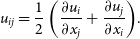
Since the centrifugal force has azimuthal symmetry, the displacement cannot depend on the azimuthal angle, so that  ${\boldsymbol{u}}={\boldsymbol{u}}(r,\theta)$, where r is the usual radial distance from the centre of the star and $\theta$ is the colatitude angle. The deformation of the star with respect to the initial configuration can be described by the strain tensor $u_{ij}$ (Love Reference Love1959), defined as
 \begin{equation}
u_{ij} = \frac{1}{2}\left(\frac{\partial u_{i}}{\partial x_{j}}+\frac{\partial u_{j}}{\partial x_{i}}\right)\!.\end{equation}
\begin{equation}
u_{ij} = \frac{1}{2}\left(\frac{\partial u_{i}}{\partial x_{j}}+\frac{\partial u_{j}}{\partial x_{i}}\right)\!.\end{equation}
This tensor accounts for the non-diagonal part of the relative deformation of the object, namely the shear, due to loading. The eigenvectors of the strain tensor form an orthonormal local basis, while the three associated eigenvalues represent the amount of deformation in the direction of the principal axis (Landau & Lifshitz Reference Landau and Lifshitz1970). Moreover, the strain tensor is very useful also for the determination of the crust breaking, via the use of the Tresca criterion (Christensen Reference Christensen2013): introducing the strain angle  $\alpha$ as the difference between the local maximum ( $\epsilon_{max}$) and minimum ( $\epsilon_{min}$) eigenvalues of the strain tensor,
 \begin{equation}
\alpha(r,\theta)=\epsilon_{Max}(r,\theta)-\epsilon_{Min}(r,\theta) ,\end{equation}
\begin{equation}
\alpha(r,\theta)=\epsilon_{Max}(r,\theta)-\epsilon_{Min}(r,\theta) ,\end{equation}
the material response to strains ceases to be elastic first in the regions of the crust where  $\alpha$ overcomes a certain threshold. According to the Tresca criterion, the material locally fails around the zone where the strain angle is peaked and this happens when
 \begin{equation*} \alpha_{Max}=\frac{\sigma_{Max}}{2} ,\end{equation*}
where  $\alpha_{Max}$ is the maximum of the function $\alpha(r,\theta)$ in the range $R'\leq r \leq R$ and $0 \leq\theta\leq\pi$, and $\sigma_{Max}$ is a property of the material called breaking strain (see, e.g., Christensen Reference Christensen2013).
To date, the value of the breaking strain in an NS crust is poorly known. Estimates of  $\sigma_{Max}$ span from values of the order of $10^{-2}\div10^{-1}$ (Horowitz & Kadau Reference Horowitz and Kadau2009; Baiko & Chugunov Reference Baiko and Chugunov2018) found by means of microscopic calculations to the much lower values of $10^{-5}\div 10^{-3}$ used in macroscopicaFootnote a models of glitches and flares (Ruderman Reference Ruderman1991; Thompson & Duncan Reference Thompson and Duncan1995). Because of these theoretical uncertainties, we will assume that a realistic value $\sigma_{Max}$ for a macroscopic portion of crustal matter is in the range ${10^{-5}\div 10^{-1}}$.
Since crustal matter is likely to be an isotropic bccPlease spell out “bcc” if needed. polycrystal, a single effective shear modulus  $\mu$ and the bulk modulus $\kappa$ are expected to be sufficient to express stresses in terms of strains via Hooke’s law (see Chamel & Haensel Reference Chamel and Haensel2008, and references therein).
The shear modulus, in particular, can be calculated as a function of the crustal composition (Ogata & Ichimaru Reference Ogata and Ichimaru1990; Horowitz & Hughto Reference Horowitz and Hughto2008). More recently, Caplan et al. (Reference Caplan, Schneider and Horowitz2018) performed classical molecular dynamics simulations where a sample of nuclear pasta at the bottom of the inner crust is deformed; they simulate idealised samples of nuclear pasta and describe their breaking mechanism, finding that nuclear pasta may be the strongest layer of an NS, with a shear modulus of  $\mu \sim 10^{30}$ erg s−1.
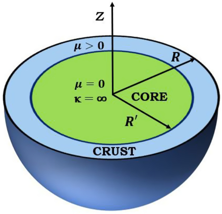
If matter is at equilibrium, the crustal composition can be thought as a function of the total density  $\rho$, and thus $\mu=\mu(\rho)$. However, continuous stratification introduces a considerable complication that can be dealt with the more refined approach proposed in Giliberti et al. (Reference Giliberti, Cambiotti, Antonelli and Pizzochero2018), which has to be solved numerically (see also Ushomirsky et al. Reference Ushomirsky, Cutler and Bildsten2000; Cutler et al. Reference Cutler, Ushomirsky and Link2003). Therefore, in order to obtain exactly solvable analytic models, in the following we will study only idealised incompressible stellar structures with homogeneous layers, implying also constant shear modulus, as sketched in Figure 1. In particular, the shear modulus is constant in the crust but zero in the core.
Sketch of the idealised non-rotating NS structure used in the present study (not in scale). The spherical configuration of radius R consists of two regions separated at  $r=R'$: the core, where the shear modulus $\mu$ is null, and the crust, where $\mu>0$. Since all the models discussed in the present work are incompressible, the bulk modulus $\kappa$ is infinite everywhere.
In the present paper, we assume that the stellar deformation can be described by the linearised theory of elasticity (Landau & Lifshitz Reference Landau and Lifshitz1970), consistently with the fact that the displacement  ${\boldsymbol{u}}$ is small. This is a reasonable assumption, since the modulus of the force acting on the body is typically very small compared to the gravitational one. As we will see in the following, in our case, the linearity assumption can be justified in retrospect by the results of Section 3. The equilibrium equation is given by
 \begin{equation} \boldsymbol{\nabla}\cdot{\boldsymbol{T}}+{\boldsymbol{F}}=0,\end{equation}
where  ${\boldsymbol{F}}$ are the external forces acting on the object and ${\boldsymbol{T}}$ is the Cauchy stress tensor, defined by Link et al. (Reference Link, Franco and Epstein1998), Franco et al. (Reference Franco, Link and Epstein2000), and Zdunik et al. (Reference Zdunik, Bejger and Haensel2008).
 \begin{equation} T_{ij} = -p \, \delta_{ij} \, + \, \sigma_{ij} = -p \, \delta_{ij} \, + \, \mu \, u_{ij}.\end{equation}
Here, p is the local pressure and  $\sigma_{ij}$ is the material incremental stress, where we made use of the incompressibility assumption $u_{ii}=0$.
3. FLE model
In this section, we study in detail the FLE model (Franco et al. Reference Franco, Link and Epstein2000), where the star is described as a homogeneous body, with a fluid core and an elastic crust of the same density. Here we present briefly only the main characteristic of the model; for the complete derivation, we refer to the original paper by Franco et al. (Reference Franco, Link and Epstein2000).
We are interested in calculating the displacement field  ${\boldsymbol{u}}$ between a configuration rotating with velocity $\Omega$ and one rotating at $\Omega-\delta \Omega$, where $\delta\Omega\,>0$ for a spinning down pulsar. The non-rotating configuration is known for our elastic star, since it coincides with the one given by the usual hydrostatic equilibrium for a fluid. Thanks to the assumed linearity of the problem, we calculate the displacements ${\boldsymbol{u}}_\Omega $ due to the spin-up of a spherical configuration to a rotating one having centrifugal potential proportional to $\Omega^2$; then, the desired displacement between the two rotating configurations is given by
 \begin{equation}{\boldsymbol{u}} = {\boldsymbol{u}}_\Omega - {\boldsymbol{u}}_{\Omega-\delta \Omega}
\,\propto \,\delta \Omega \, \Omega .\end{equation}
\begin{equation}{\boldsymbol{u}} = {\boldsymbol{u}}_\Omega - {\boldsymbol{u}}_{\Omega-\delta \Omega}
\,\propto \,\delta \Omega \, \Omega .\end{equation}
Clearly this procedure gives results identical to the method described by Franco et al. (Reference Franco, Link and Epstein2000), according to which the displacement field  ${\boldsymbol{u}}$ up to the linear order in $\delta\Omega$ is
 \begin{align}\begin{split} u_{r} (r,\theta) & = \left(a r-\frac{1}{7}Ar^{3}-\frac{1}{2}\frac{B}{r^{2}}+\frac{b}{r^{4}}\right) P_{2}\equiv f(r)P_{2}, \\ u_{\theta}(r,\theta) & = \left(\frac{1}{2}a r-\frac{5}{42}Ar^{3}-\frac{1}{3}\frac{b}{r^{4}}\right)\frac{dP_{2}}{d\theta} , \end{split}\end{align}
where  $P_{2}=\frac{1}{2}\left(3 \cos^{2}\theta-1\right)$ is the second Legendre polynomial of argument $\cos \theta$ and we have defined the function f(r). The four coefficients a, b, A, and B are fixed by four boundary conditions, two at the core–crust transition radius $r=R'$ and two at the star’s surface $r=R$. At both these interfaces, we have to require the continuity of radial stresses, $T_{rr}=-p+\mu u_{rr}$, and that $\sigma_{r\theta}=0$, since both the fluid core and the vacuum outside the star cannot support shears. It is useful to introduce the sound speed in the crust of transverse waves, $c_{t}=\sqrt{\mu/\rho}$, and the usual Keplerian velocity, $v_{K}=\sqrt{GM/R}$, so that the four boundary conditions read
 \begin{align}\begin{split} & a-\frac{8}{21} A R^{2} - \frac{B}{2R^{3}}+\frac{8}{3}\frac{b}{R^5} = 0, \\ & a-\frac{8}{21}A R'^{2} - \frac{B}{2R'^{3}}+\frac{8}{3}\frac{b}{R'^5} = 0, \\ & \frac{df}{dr}(R) +\frac{1}{5}\frac{v_{K}^{2}}{c_{t}^{2}}\frac{f(R)}{R}-\frac{1}{3}\frac{\Omega\delta\Omega}{c_{t}^{2}}R^{2} = -\frac{A R^{2}}{2}+\frac{B}{R^3},\\ & \frac{df}{dr}(R') = -\frac{1}{2}\left(A R'^2 + \frac{B}{R'^{3}}\right) , \end{split}
\end{align}
\begin{align}\begin{split} & a-\frac{8}{21} A R^{2} - \frac{B}{2R^{3}}+\frac{8}{3}\frac{b}{R^5} = 0, \\ & a-\frac{8}{21}A R'^{2} - \frac{B}{2R'^{3}}+\frac{8}{3}\frac{b}{R'^5} = 0, \\ & \frac{df}{dr}(R) +\frac{1}{5}\frac{v_{K}^{2}}{c_{t}^{2}}\frac{f(R)}{R}-\frac{1}{3}\frac{\Omega\delta\Omega}{c_{t}^{2}}R^{2} = -\frac{A R^{2}}{2}+\frac{B}{R^3},\\ & \frac{df}{dr}(R') = -\frac{1}{2}\left(A R'^2 + \frac{B}{R'^{3}}\right) , \end{split}
\end{align}
Using the definition (7) and the boundary conditions (8), the four coefficients a, b,A, and B are obtained with straightforward algebra.
It is useful to rewrite the displacement (7) as
 \begin{align} \begin{split} u_{r} & = \frac{\Omega \, \delta\Omega\,R^{3}}{Q(c_{t},v_{K},L)} \, \left(\frac{\skew4\tilde{a} r}{R}-\frac{\skew2\tilde{A} r^{3}}{7 R^{3}}-\frac{\skew4\tilde{B} R^{2}}{2 r^{2}}+\frac{\skew2\tilde{b} R^{4}}{r^{4}}\right) P_{2}, \\ u_{\theta} & = \frac{\Omega \, \delta\Omega\,R^{3}}{Q(c_{t},v_{K},L)} \, \left(\frac{\skew4\tilde{a} r}{2 R}-\frac{5 \skew2\tilde{A} r^{3}}{42 R^{3}}-\frac{\skew2\tilde{b} R^{4}}{3 r^{4}}\right) \frac{dP_{2}}{d\theta}, \end{split} \end{align}
where the tilde superscript indicates that now the coefficients are dimensionless: all the dependence on the physical parameters has been included into the pre-factors. In particular, in the above expressions the parameter Q, which has the dimension of a squared velocity, is a complicated function of the physical parameters of the problem (see equation (10) and Appendix B for its explicit form). On the other hand, the coefficients  $\skew4\tilde{a}$, $\skew2\tilde{A}$, $\skew2\tilde{b}$, and $\skew4\tilde{B}$ are functions of the parameter $ L = R' / R $ only, where the limits $L=0$ and $L=1$ describe a completely solid star and a completely fluid star, respectively. Since the parameter L spans from about $0.86$ to $0.95$ when realistic EoS Please spell out “EoS” at first use, if needed.are used, the parameter $q=1-L$ is sufficiently small to consider the expansion of the coefficients $\skew4\tilde{a}$, $\skew2\tilde{b}$, $\skew2\tilde{A}$, $\skew4\tilde{B}$, and Q only up to the second order in q. The boundary conditions (8) fix the form of the dimensionless coefficients in (9), that turn out to be
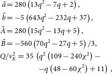 \begin{align} \begin{split}\skew4\tilde{a}& = 280 \left( 13 q^2 - 7 q + 2 \right),\\ \skew2\tilde{b}& = -5 \left( 643 q^2 - 232 q + 37 \right),\\ \skew2\tilde{A}& = 280 \left( 15 q^2 - 13 q + 5 \right),\\ \skew4\tilde{B}& = - 560 \left( 70 q^2 - 27 q + 5 \right) / 3, \\ Q & / v_K^2 = 35 \, \left( q^2 \left(109-240 \chi^{2} \right) - \right. \\ & \qquad \qquad \left. - q \left( 48 - 60 \chi^2 \right) +11 \right) , \end{split}\end{align}
where  $\chi$ is defined as the ratio between the sound speed in the crust $c_t$ and the star’s Keplerian velocity $v_K$,
 \begin{equation} \chi\, = \, \frac{c_t}{v_K} \, \ll \, 1 . \end{equation}
We interpret the parameter  $\chi$ as an indicator of the relative importance of the elastic forces with respect to the unperturbed gravitational one: in this sense, this ratio gives an estimation of the goodness of the linear perturbation theory. According to current estimates of $\mu \sim 10^{28}$ erg cm−3, $\chi$ is expected to be much less than unity in the whole crust (see, e.g., Figure 7 of Zdunik et al. Reference Zdunik, Bejger and Haensel2008). Interestingly, as noted by several authors (see, e.g., Haskell et al. Reference Haskell, Jones and Andersson2006; Bastrukov et al. Reference Bastrukov, Chang, Takata, Chen and Molodtsova2007), the speed of transverse elastic shear waves $c_t \sim 10^{8}\,$cm/s is rather constant (within a factor of 2) throughout the crust, so that we expect $\chi \sim 10^{-2}$.
3.1. Parametric study of the FLE model
In their original work, Franco et al. (Reference Franco, Link and Epstein2000) considered only a ‘standard’ NS of mass  $M=1.4 M_{\odot}$, $R=10\,$km and $R'=0.95\,R$ (i.e. $L=0.95$ according to the present notation), as benchmark stellar configuration. Here, we extend their analysis investigating the behaviour of the FLE model as a function of the star’s parameters: radius, mass, and crust thickness.
First, we consider the displacement (9). We define a dimensionless weight factor W that quantifies the displacement at a given radial coordinate for a given amount of spin-down  $\delta\Omega$, namely
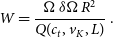 \begin{align} W=\frac{\Omega \, \delta\Omega\,R^{2}}{Q(c_t,v_K,L)}.\end{align}
To gain some physical understanding of how W scales with the stellar parameters, we use the smallness of the  $\chi$ and q parameters in equation (10), which gives a rough estimate of Q as
 \begin{equation} Q \approx 385 \, v_K^{2} .\end{equation}
Moreover, to remove the dependence of the numerator on a particular set of rotational parameters, we can fix  $\Omega$ and $\delta\Omega$ to some constant value. In this way, all the remaining contributions to W will depend on the structural properties of the star. Hence, using the approximation (13) into (12) immediately gives that the displacements in (9) are expected to scale with the inverse of the average density of the star,
 \begin{equation}W \propto \frac{R^{2}}{v_K^{2}}= \frac{R^3}{GM} \propto \frac{1}{\rho} .\end{equation}
This tells us that the FLE model predicts smaller displacements for dense stellar configurations.
For a better understanding of this behaviour, the strain angle  $\alpha$ may be calculated changing the parameters one by one, keeping fixed all the others. For comparison purposes, we set the relative extension of the core to be $L=0.95$, the same used in the original FLE study. The procedure used to calculate the strain angle is as follows. First, the relations in (9) are used to obtain the components of the strain tensor in spherical coordinates. At this point, for a fixed value of the coordinates r and $\theta$, we calculate numerically the eigenvalues of the strain tensor, so that the definition in (3) can be locally applied.
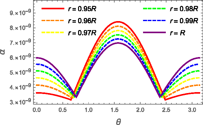
Since the displacements, and thus the strain, are proportional to the actual spin-down between the two configurations, we set the pre-factor  $\Omega\delta\Omega$ equal to one for simplicitybFootnote b. Therefore, to calculate the deformation for a certain star, it is just sufficient to multiply the desired quantities for the actual parameter $\Omega \, \delta\Omega$. The strain angle, being a local quantity, depends on the position inside the crust; for given mass, radius, and crust thickness of the star, it is shown in Figure 2, where it is possible to observe that $\alpha$ is a decreasing function of r. Hence, we expect that, if the crust breaks, the failure threshold will be reached first at the crust–core interface, near the equatorial plane (i.e. $\theta \approx \pi/2$ in our coordinates). However, the value obtained with this test configuration is by far smaller than the smallest breaking strain theoretically expected of $10^{-5}$. As we will see, this kind of behaviour is scarcely influenced by the model used.
Strain angle as a function of the colatitude  $\theta$ for the FLE model and fixed benchmark values $M=1.4M_{\odot}$, $R=10\,$km, and $L=0.95$. The strain angle is calculated for different values of the radius: $r=R$ (purple), $r=0.99 R$ (blue), $r=0.98 R$ (green), $r=0.97 R$ (yellow), $r=0.96 R$ (orange), and $ r=0.95R$ (red). In particular, we indicate with a solid line the innermost (red) and outermost (purple) value of $\alpha$, and a dashed line for the others. We used $\Omega\delta\Omega =1\,$rad2 s−2.
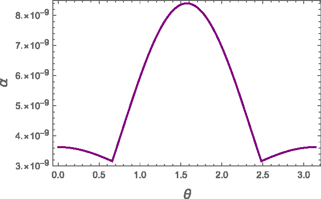
Moreover, by looking at equations (9) and (14), we see that deformations depends mainly on the radius and on the mean density of the star. In this sense, it is interesting to compare the strains of stars all having the same average density  $ \rho \, = \, 3 M/(4\pi R^{3}), $ but different radii and masses. We find that, as long as the density is taken constant but the mass and the radius vary, the strain is nearly unchanged. An example of this is shown in Figure 3, where we fixed $\rho$ to be the average density of a star of $1.4 \, M_\odot$ and $R=10\,$km: different choices of the mass and of the radius that are consistent with the fixed density value do not move the estimated strains, providing a numerical check of the goodness of the approximation made in equation (14). This result indicates that, in the original FLE model, the strain developed by a spinning-down pulsar (for a given value of $\Omega\delta\Omega$) depends essentially only on the average density of the star and on L: the independent choice of both M and R implies a degeneracy in the results.
Strain angle  $\alpha$ of the FLE model restricted to the spherical shell $r=R'$ as a function of the colatitude $\theta$. The crust thickness parameter is fixed to $L=0.95$, but we consider two extreme values of the stellar radius: $R=10\,$km and $R=20\,$km. The corresponding two masses M are fixed by the constraint that the average density of both configurations is $\rho=6.6\times10^{14}\,$g cm−3. The two curves appear to be superimposed in the graph.
From the M–R relation of realistic equations of state, we know that more massive stars typically have smaller radii, implying a larger average density and smaller W, as can be seen in equation (14). In this sense, we can say that in the original FLE model, heavier stars develop smaller strains during the spin-down, which is the expected behaviour considering that the centrifugal force is less effective on more compact stellar configurations.
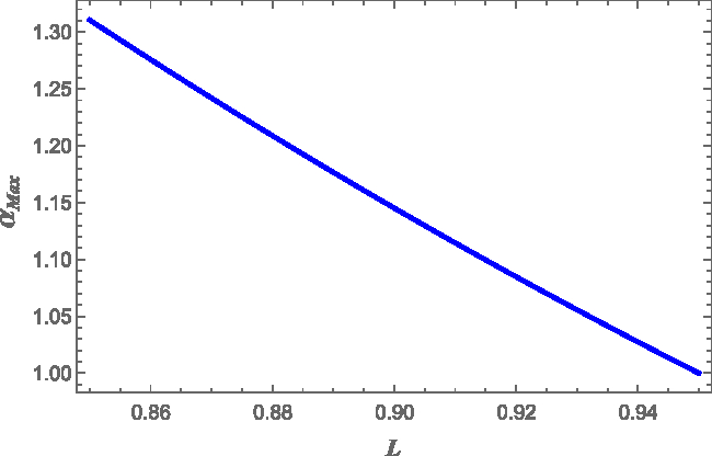
Finally we can study also how the value of L affects  $\alpha$. We find that the strain angle is a weakly increasing function of the crustal thickness, that is, a decreasing function of L in the range $0.85\leq\, L\,\leq0.95$. This can be seen in Figure 4, where we computed the maximum value of $\alpha(L)$ over $\theta$, for $r=R'$ and $M=1.4M_{\odot}$ and $R=10$ km (in particular $\alpha_{Max}(L = 0.85) \simeq 1.3 \alpha_{Max}(L = 0.95)$). Figure 4 shows clearly that a thick crust can support larger deformations with respect to a thinner one (as expected), but the dependence is not so strong. The reason is that the elastic restoring force is small compared to the gravitational one (11).
The maximum strain angle as a function of the thickness parameter  $L=R'/R$ for the FLE model. The fixed benchmark values $M=1.4M_{\odot}$ and $R=10\,$km have been used. The strain angle is normalised at the value reached for $L=0.95$ and calculated at the core–crust interface $r=R'$. We used $\Omega\delta\Omega =1\,$rad2 s−2.
3.2. Cowling approximation
It is possible to exploit the FLE model as a tool to estimate the impact of the Cowling approximation (Cowling 1941), according to which the perturbation of the star’s gravitational potential is neglected. This kind of approach has been widely used in the literature, especially for the study of the oscillation modes of NSs (McDermott et al. Reference McDermott, Van Horn and Hansen1988), but also for static deformations (Ushomirsky et al. Reference Ushomirsky, Cutler and Bildsten2000; Johnson-McDaniel & Owen Reference Johnson-McDaniel and Owen2013). In fact, this approximation has the advantage to simplify considerably the momentum equations and to avoid the need to solve the perturbed Poisson equation. However, it has a large impact on the estimation of elastic deformations, as we show in the following.
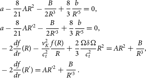
The Cowling approximation can be easily implemented by setting  $\delta\phi=0$ in the perturbed equations of the original FLE model [in particular in equations (12) and (31) of Franco et al. (Reference Franco, Link and Epstein2000)]. Assuming this further simplification, we can now rewrite the boundary conditions in (8) as
 \begin{align}\begin{split} & a-\frac{8}{21} A R^2 - \frac{B}{2 R^3} + \frac{8}{3} \frac{b}{R'^5} =0, \\ & a-\frac{8}{21} A R'^{2} - \frac{B}{2 R'^3} + \frac{8}{3} \frac{b}{R'^5} =0, \\ & -2 {\frac{df}{dr}(R)} - \frac{ v_K^2 }{ c_t^2 } \frac{ f (R) }{R}+\frac{2}{3}\frac{ \Omega \delta \Omega }{c_t^2} R^2 = A R^2+\frac{B}{R^3}, \\ & -2 {\frac{df}{dr}(R')} = AR'^2+\frac{B}{R'^3} .\end{split}\end{align}
Using definition (7), together with the solutions of the above equations, we obtain the corresponding displacement introduced in (9). The explicit form of the coefficients is given in Appendix B; see (57). The simplest way to estimate the net effect of the perturbed gravitational potential is to neglect the terms containing the ratio  $\chi$ and compare the displacement obtained with and without the Cowling approximation, indicated as ${\boldsymbol{u}}^{C}$ and ${\boldsymbol{u}}$, respectively. In the limit $\chi \, =\,0$, we find that
 \begin{equation} \frac{u_{r}}{u_{r}^{C}} = \frac{u_\theta}{u_{\theta}^{C}} = \frac{5}{2} \, + \, O\left( \, \chi^2 \,(1-L) \, \right) .\end{equation}
Therefore, in the FLE scheme, the displacements calculated with the Cowling approximation are 40% of the ones calculated by considering also the gravitational potential perturbation (see also Appendix B).
3.3. FLE model with M–R relation from realistic equations of state
In the previous section, we analysed the main physical properties of the FLE model by using only benchmark values for R,L, and M. In this section, instead, we will study the strain developed in rotating NSs by using the mass–radius relation of two very different equations of state, the soft SLy (Douchin & Haensel Reference Douchin and Haensel2001) and the stiff GM1 (Glendenning & Moszkowski Reference Glendenning and Moszkowski1991).
This use of realistic EoSs, albeit still quite approximate in this case of uniform density, links all the parameters of the star (i.e. R, L, and  $\rho$) to its mass M. Given the EoS, by solving the hydrostatic equilibrium equations (namely, the Tolman–Oppenheimer–Volkoff (TOV) equations), we obtain the mass–radius relation R(M). At this point, the star is continuously stratified, but to use the FLE model, we choose the average uniform density $\rho(M)$ as
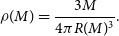 \begin{equation}\rho(M)=\frac{3M}{4\pi R(M)^3}. \end{equation}
Furthermore, also the parameter L can be determined for a given EoS and total stellar mass: solving the TOV equations, we find the radius R´(M) corresponding to the crust–core density transition of the particular EoS under study, so that we can fix  $L(M) = R'(M)/R(M)$.
This approach simplifies our parametric study, since once the stellar mass is chosen the same applies self-consistently for all the other parameters and, at the same time, it gives a better estimate of what we might expect in an astrophysical scenario.
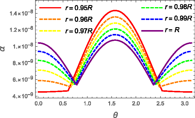
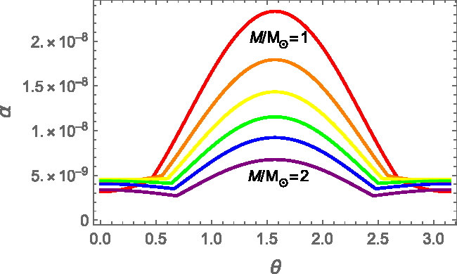
In Figures 5 and 6, we show, respectively, the strain angle  $\alpha(r,\theta)$ calculated for a $1.4M_{\odot}$ NS at different radii and the one calculated at $r=R'$ for different stellar masses by using the relation given by the EoSs. As expected from the previous analysis, the strain is a decreasing function of the radius and of the mass.
Strain angle  $\alpha$ as a function of the colatitude for the original FLE model. The strain is calculated for $M=1.4M_{\odot}$, with the SLy EoS, at different evenly spaced values of r, from $r=R'$ (red) to R (purple). In particular, we indicate with a solid line the innermost and outermost values of $\alpha$, and a dashed line for the others. Again, the maximum strain occurs at the core–crust interface on the equatorial plane.
Strain angle  $\alpha$ as a function of the colatitude for the original FLE model on a spherical shell of radius $r=R^{'}$, that is, where the strain angle reaches its maximum value. The structural parameters have been fixed by considering the SLy EoS, for different stellar masses: $M=1M_{\odot}$ (red), $M=1.2M_{\odot}$ (orange), $M=1.4M_{\odot}$ (yellow), $M=1.6M_{\odot}$ (green), $M=1.8M_{\odot}$ (blue), and $M=2M_{\odot}$ (purple).
On the other hand, it is interesting to compare the maximum strain angle  $\alpha_{Max}$ calculated with different EoSs. In Figure (7), we compare the relatively soft SLy Eos with the stiffer GM1, which leads us to conclude that a stiffer equation of state gives larger maximum values of $\alpha_{Max}$. Again, this is has to be expected from (14); for the same stellar mass, a stiffer EoS gives a larger stellar radius, and thus a smaller compactness. Therefore, the numerical analysis confirms the qualitative picture that is expected from equation (14); however, from the quantitative part of view, the use of more realistic combination of parameters, given by the use of the EoS, give larger strains with respect with the standard configuration ( $M=1.4M_{\odot}$, $R=10$ km) chosen by Franco et al. (Reference Franco, Link and Epstein2000).
Comparison of the maximum values of the strain angle  $\alpha_{Max}$ (which always occurs at $r=R^{'}$ and $\theta=\pi/2$), obtained with the original FLE model, as function of the stellar mass. A comparison between the SLy EoS (blue) and GM1 EoS (red) is made for our benchmark value $\Omega\delta\Omega=1\,$rad2 s−2. The green star indicates the maximum strain value obtained for the standard configuration used in Franco et al. (Reference Franco, Link and Epstein2000) with $M=1.4M_{\odot}$, $R=10$ km, and $L=0.95$ (red curve of fig:STRAIN TUTTO VARIABILE DIVERSI RAGGI). The curves approach for higher masses as the crust thickness decreases and R’ gets closer to R; the GM1 line remains always well above SLy because a stiffer equation of state gives a thicker crust for the same mass.
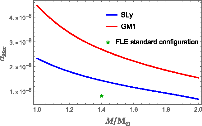
The most important information that can be extracted from Figure 7 is that the maximum strain value (of the order of  $\alpha_{Max} \sim 10^{-8}$) is three orders of magnitude smaller than the lowest allowed breaking strain ( $\sigma_{Max} \sim 10^{-5}$), when $\Omega\delta\Omega=1 \mathrm{rad^2~s^{-2}}$. Therefore, according to the FLE model, it’s unlikely that the spin-down between two subsequent glitches could deform the crust enough to break it: the only viable possibility is that the crust is always in a stressed state, near the failure threshold. This result accords with the observational finding of a lack of correlation between glitch sizes and waiting times: although this may seem counterintuitive if glitches are threshold-triggered events (as in theories involving starquakes or superfluid vortex avalanches), the lack of correlation can emerge naturally when a threshold mechanism is combined with the secular stellar braking, as shown by Melatos et al. (Reference Melatos, Howitt and Fulgenzi2018).
It is possible to give a rough estimate of the average spin-down  $\delta\Omega$ that occurs between two glitches in a pulsar: given the spin-down rate $\dot \Omega<0$ and the average waiting time between glitches $\delta t$, we set $\delta\Omega\, =\, |\dot \Omega|\,\delta t$.
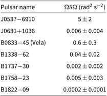
In Table 1, the specific values of  $\Omega\delta\Omega$ are reported for a selection of pulsars with at least 10 recorded events. Clearly, the most interesting pulsars for the present analysis are the ones with large values of the product $\Omega\, |\dot \Omega|\,\delta t $; the record holder is J0537-6910, followed by the Vela pulsar. As we can see, except for the Vela and J0537-6910, the actual rotational parameters can only decrease the values for the strain amplitude discussed above (that were all calculated for $\Omega\delta\Omega=1\,$rad2 s−2). The strain remains well below the critical threshold even in the limit of very light stars with stiff equation of state. Furthermore, if we consider the highest current estimate of the breaking strain value $\sigma_{max} \sim 0.1$, we generally will not expect the crust to break via the spin-down mechanism in the whole star life, as has been recently proposed by Fattoyev et al. (Reference Fattoyev, Horowitz and Lu2018).
The rotational parameter  $\Omega\delta\Omega$ that sets the actual value of the average stress developed in between two glitches is given for a selection of pulsars with at least 10 glitches. Data are taken from the Jodrell Bank Glitch Catalogue (www.jb.man.ac.uk/pulsar/glitches.html, see also Espinoza et al. Reference Espinoza, Lyne, Stappers and Kramer2011).
Finally, we can also compare the maximum strain angle using the original FLE approach ( $\alpha_{FLE}$) with the one obtained by using the homogeneous model of Baym and Pines ( $\alpha_{BP}$), where the star is described as an elastic, rotating, homogeneous spheroid: this is simply obtained by considering the limit $R'=0$ of the FLE model. We choose $M=1M_{\odot}$, and calculate all the other quantities according to the SLy equation of state, since the use of a light and soft star emphasises differences (however, we observe that the same analysis can be done with the GM1 EoS or using some fiducial values for the stellar configuration, with analogous results). Both $\alpha_{FLE}$ and $\alpha_{BP}$ are evaluated for the same radius r, that is the one of core–crust transition for a star obtained with the SLy EoS ( $\rho_{core-crust}=1.3\times 10^{14}\mathrm{g~cm^{-3}}$), and $\theta=\pi/2$, where the strain angle is maximum. In this case, we obtain very similar values for the two models:
 \begin{align*}& \alpha_{BP}=2.33\times10^{-8}, \\ & \alpha_{FLE}=2.55\times10^{-8}. \end{align*}
This result leads us towards another further step: the study of an FLE-like model in which the crust and the core can have different average densities.
4. Two-densitymodel
The original FLE model provides a useful tool to estimate the deformation of a rotating NS in Newtonian gravity, but it is based on the strong assumption that the star must have the same constant density everywhere. In this section, we show how to overcome this limitation, by using a self-consistent approach, where the NS is divided in two homogeneous layers representing the fluid core and the crust, with densities  $\rho_{f}$ and $\rho_{c}$, respectively. As we will show, the self-consistency of the model becomes manifest in two additional conditions for the gravitational potential. Note, in fact, that contrary to the FLE model here one cannot use the knowledge of the gravitational potential of a perturbed homogeneous spheroid, but has to calculate it self-consistently by solving the perturbed Poisson equation.
The present analysis is based on the more general result discussed by Vermeersen et al. (Reference Vermeersen, Sabadini and Spada1996), where it is shown that it is possible to develop and build analytical models containing a large number of layers as a description of auto-gravitating rocky planets. Here this set of ideas is adapted to the rotating NS problem. In particular, the present approach takes inspiration from the two-layer model firstly developed by Sabadini et al. (Reference Sabadini, Yuen and Boschi1982) in the context of viscoelastic planets (like Earth).
In this section, we only discuss the general features of the model. Detailed derivation of the model and of the main equations are summarised in Appendix A, while more technical details can be found in Sabadini et al. (Reference Sabadini, Vermeersen and Cambiotti2016) and in the recent description of a class of more realistic (i.e. continuously stratified and auto-gravitating) NS models (Giliberti et al. Reference Giliberti, Cambiotti, Antonelli and Pizzochero2018).
In our two-density model, we find that the displacement  ${\boldsymbol{u}}$ still has the same analytic form of the displacement given in equation (7); this is not surprising as the main difference with respect to the original FLE model lies in the treatment of the boundary conditions. In fact, at $r=R'$ we have a finite density discontinuity between the core and the crust, a detail which has to be carefully incorporated into the analysis of the crust–core interface. As a consequence, if we write down the displacement ${\boldsymbol{u}}$ in the form of equation (9), the four coefficients $\skew4\tilde{a}$, $\skew2\tilde{b}$, $\skew2\tilde{A}$, and $\skew4\tilde{B}$ will be functions not only of the thickness L and of $\chi$, but also of the density ratio
 \begin{equation} d=\frac{\rho_{c}}{\rho_{f}}<1. \end{equation}
As for the previous model, a simplified form for the coefficients  $\skew4\tilde{a}$, $\skew2\tilde{A}$, $\skew2\tilde{b}$, and $\skew4\tilde{B}$ is given in Appendix B (the complete and exact form of the coefficients turns out to be much more complex with respect to the previous cases).
4.1. A first comparison with the original FLE model
We start by pointing out that the original FLE model can be obtained as a trivial limit  $d = 1$ of our two-density model. In fact, imposing $d=1$ in our model, we calculate the resulting displacement ${\boldsymbol{u}}$ and the analogous one (i.e. by using the same values of L, R, M, and $\chi$) with the FLE model, ${\boldsymbol{u}}^{FLE}$. The ratio between the two gives
 \begin{equation}\frac{u_r}{u^{FLE}_r}\, =\,\frac{u_\theta}{u^{FLE}_\theta}\, =\, 1 \,\,\mathrm{for}\,\,d=1 .\end{equation}
In other words, our model can be seen as a complete generalisation of FLE approach, accounting in a self-consistent way for two different density in the NS core and crust.
We now follow the same analysis done for the FLE model in the previous section, varying in turn one parameter while keeping the others fixed. Since the parameter space is rather large, we will vary several parameters at the same time by using a realistic EoS in the next subsection. However, as a preliminary example, we make a comparison with the FLE model by studying a situation similar to the one described in Figure 2, which corresponds to a star with  $R=10$ km and mass $M=1.4M_{\odot}$: in Figure 8, we plot the strain at different radii for the two density model, using some fiducial values of the parameters involved, with $\rho_f\approx 6.6\times10^{14}\,$g cm−3 and $d=0.1$, such that the total mass is still of $1.4\,M_\odot$. Firstly, we note that the strain angle in this case is larger with respect to the FLE one. Furthermore, as the radial dependence of $\alpha(r,\theta)$ shows, the strain angle reaches its maximum value $\alpha_{Max}$ at the crust–core interface. However, differently with respect to the FLE model, in this case the value of the strain is highest at the poles.
(Top) Strain angle as a function of the colatitude  $\theta$ for the two-density model and fixed benchmark values $M=1.4M_{\odot}$, $R=10\,$km, $L=0.95$, $\rho_f=6.6\times10^{14}$, and $\rho_c=\rho_f/10$. The strain angle is calculated for different values of the radius: $r=R$ (purple), $r=0.99 R$ (blue), $r=0.98 R$ (green), $r=0.97 R$ (yellow), $r=0.96 R$ (orange), and $ r=0.95R$ (red). In particular, we indicate with a solid line the innermost and outermost values of $\alpha$, and with a dashed line the others. We used $\Omega\delta\Omega=1\,$rad2 s−2. (Bottom) Log-scale comparison of the strain angle calculated for the same configuration ( $M=1.4M_{\odot}$, $R=10\,$km, $L=0.95$, $r=R'$) using the FLE (blue, dashed) and the two-density (red) models.
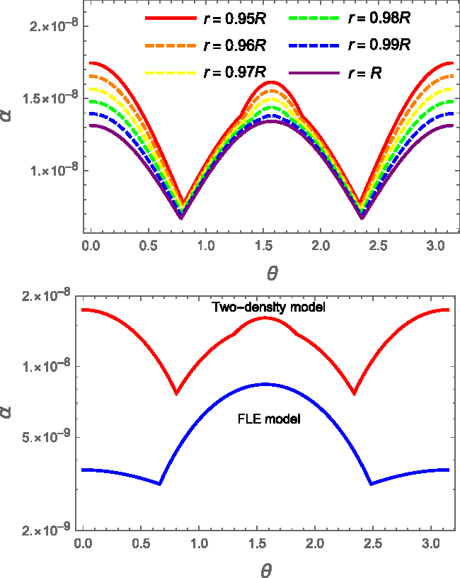
As a first check, we set  $\rho_{f}=\rho_{c}$ in the two-density model and we find, as expected, that the maximum strain is placed at the equator (19). Therefore, the stratification (i.e. the presence of layers with different densities) introduces a new degree of freedom into the model, so that it is possible to move the region of maximum stress away from the equator.
Furthermore, we observe that, although the values of the strain angles obtained with the new model are larger than the one of the FLE approach,  $\alpha$ is still well below the minimum breaking threshold of $10^{-5}$.
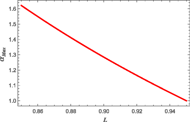
As a final comparison, despite the fact that  $\alpha$ is still a decreasing function of L, we note that the crust thickness has a larger impact on the strain value with respect to the FLE model. In this case, we find that $\alpha_{Max}(L=0.85)/\alpha_{Max}(L=0.95)\simeq1.6$ for a $1.4\,M_{\odot}$ NS with $d=0.1$ (cf. with the factor $1.3$ in Figure 4). This can be seen in Figure 9, where the strain angle, computed for a fixed stellar configuration, is shown as a function of the thickness parameter L.
The maximum strain angle as a function of the thickness parameter  $L=R'/R$ for the two-density model and fixed benchmark values $M=1.4M_{\odot}$, $R=10\,$km, and $d=0.1$ (cf. with Figure 4). The strain angle is normalised at the value reached for $L=0.95$ and calculated at the core–crust interface $r=R'$. We used $\Omega\delta\Omega =1\,$rad2 s−2.
4.2. Realistic equations of state
As already done for the FLE model in Section 3.3, we investigate the behaviour of the two-density model by imposing that not all the parameters present in the equations are free: they have to satisfy the constrain which arises by the fact that an EoS for the internal matter is related to a particular mass–radius relation. In order to give a stricter comparison with the FLE’s model, and since the crust contains only a small percentage of the total stellar mass, we use this simple prescription
 \begin{equation}\rho_{f}\simeq\frac{M}{4/3\pi R^3}.\end{equation}
On the other hand, the exact value of d, whose definition is in equation (18), is found by the appropriate relation due to the particular EoS that has been chosen and therefore is a known function of the stellar mass. The crust density is assumed to be
 \begin{equation}\rho_{c}=d \, \rho_{f}\simeq d\frac{M}{4/3\pi R^{3}} ,\end{equation}
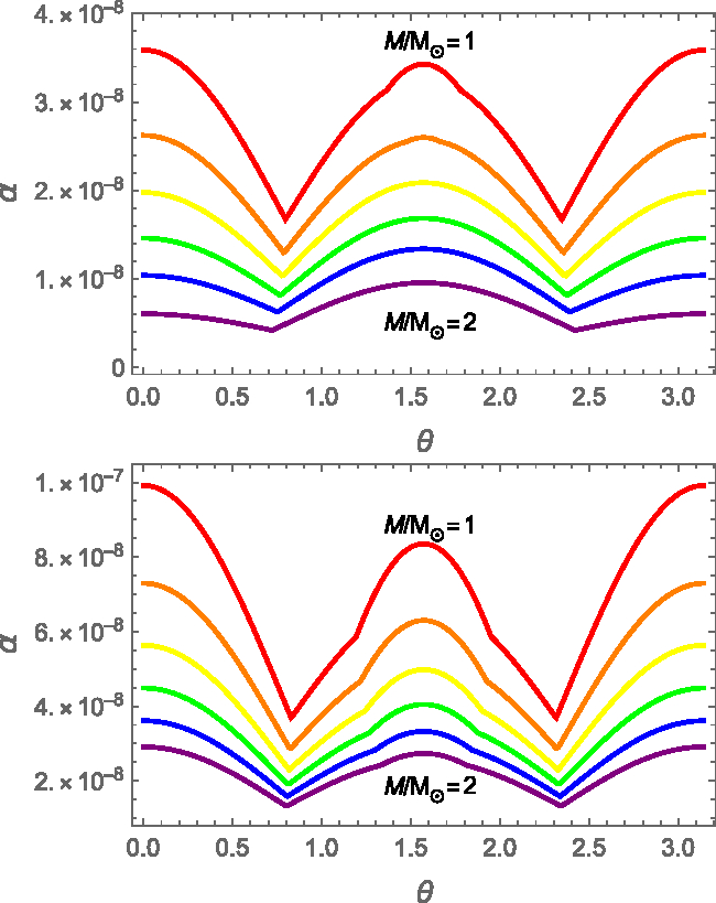
a prescription that is used in both in Figures 10 and 11. In Figure 10, the strain angle at the core–crust interface is shown for different stellar masses. As expected, also in this case we have that the strain decreases when the total mass is increased: again, heavier stars have smaller radii and higher density, and are thus more difficult to deform. However, we highlight the new interesting feature that never arises by using the original FLE model: the maximum strain  $\alpha_{Max}$ is now, in most of the cases, at the poles. Interestingly, for the softer EoS and for heavier objects, there are also cases where the maximum is still at the equator. Here, in fact, the crust is extremely thin, and the strain tends to resembles the LFE behaviour. However, when the opposite is true, the crust gains a great importance in the strain shape, bringing the maximum at the poles.
Strain angle at  $r=R^{'}$ as a function of the colatitude $\theta$ for the two-density model and different masses: $M=1M_{\odot}$ (red), $M=1.2M_{\odot}$ (orange), $ M=1.4M_{\odot}$ (yellow), $M=1.6M_{\odot}$ (green), $M=1.8M_{\odot}$ (blue), and $M=2M_{\odot}$ (purple). The stellar structural parameters are fixed by using the SLy EoS in the upper panel, while GM1 was used for the lower one.
Maximum strain angle  $\alpha_{Max}$ (which occurs at the core–crust interface) as a function of the stellar mass for the FLE (solid curves) and for the two-density model (dashed curves). The red curves refer to the GM1 equation of state, and blue curves to SLy.
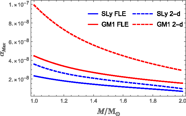
Finally, in Figure 11 we compare the maximum strain angle  $\alpha_{Max}$ as function of the stellar mass, calculated with the FLE and the two-density model, using both SLy and GM1 EoSs. Again, stiffer EoS gives larger strain, as discussed above. The use of our model allows to get larger strains that are typically two times larger than the ones obtained with FLE model. As noted above, however, in both the scenarios the maximum strain angle is still far even from the minimum breaking strain value of $\sim\!\!10^{-5}$. Therefore, the analysis with this two-density model confirms that, starting from an unstressed configuration, the deformation due only to the inter-glitch spin-down is not large enough to trigger a starquake.
5. Conclusion
In this work, we studied in details two different models describing the deformation of the crust of a rotating NS due to its spin-down. The first is the original FLE model (Franco et al. Reference Franco, Link and Epstein2000) describing an uniform star, with a fluid core and an elastic crust. The second is our two-density generalisation, based on an adaptation of the scheme first proposed by Sabadini et al. (Reference Sabadini, Yuen and Boschi1982) for the study of rocky planets deformations. Despite the fact that both approaches are analytically solvable, the scheme proposed by Sabadini et al. (Reference Sabadini, Yuen and Boschi1982) has two main advantages: it is self-consistent for spherical auto-gravitating bodies (i.e. not only homogeneous ones) and partially accounts for stratification as it allows for two different densities in the core and in the crust.
Both schemes were introduced in the literature without a specific parameter study: the FLE model, for example, was originally built for the study of pulsars precession, and solved only for a fiducial stellar configuration (see, e.g., Figure 7), while in the original work of Sabadini et al. (Reference Sabadini, Yuen and Boschi1982), the focus was on geophysical applications. Here, instead, we studied how the calculated strains vary by considering different stellar structures, where parameters such as the radius, the average density, and the crust thickness are linked to the mass via an EoS. In order to parametrise our ignorance on the unknown equation of state for matter at supra-nuclear densities, an important part of the analysis has been performed employing SLy and GM1 as a prototype of a soft and a stiff EoS, respectively.
Three main conclusions have been drawn. First, all models [including the homogeneous limit of Baym & Pines (Reference Baym and Pines1971)] indicate that more compact stars are more difficult to deform (the strain scales with the inverse of the average density). Because of this quite general scaling, SLy is found to give smaller strains than GM1, as it gives rise to more compact configurations.
Secondly, we found that the two-density model gives a strain angle that is about two times larger than the FLE one, although the dependence of the strain on various physical quantities is qualitatively the same in both models. This clearly indicates that the different density values of the core and crust is a fundamental aspect for the determination of the displacement and stress in rotating NS.
As a third point, the maximum strain angle obtained using the two-density model (as shown in Figure 11) varies for less than one order of magnitude according to the present analysis (the maximum strain for an NS of  $M=1\,M_{\odot}$ is only about $\simeq2\div3$ times the one of an NS with $M=2\,M_{\odot}$, depending on the EoS used). Hence, it is not possible to conclude that the mass is a key parameter which clearly divides NSs in light objects that can easily undergo crust failure and compact ones that are much more difficult to break.
Furthermore, the modification of FLE model, with the introduction of the Cowling approximation, gives us a clear analytic proof of how strong this assumption can be on the calculation of the displacement  ${\boldsymbol{u}}$. In fact, we showed that the displacement field, and thus the strain, is 40% of the original one. This suggests some warnings about the use of such approximation for the study of elastic displacements in NS.
As a first, simple, astrophysical application of our two-density model, we selected a group of pulsars that have been observed to glitch several times and we gave an estimate of the strain angle due to the spin-down between subsequent events. Both the FLE and the two-density models clearly indicate that starting from an initial unstressed state, it is not possible to develop enough strain to break the crust as frequently as glitches are observed. Therefore, the idea of a starquake as a trigger for the vortex avalanche in glitches of superfluid NSs is severely challenged, unless the crust is always in a state of great internal stresses (which is actually the case for the Earth and other rocky planets). Moreover, the finding that the maximum strain reached from a relaxed state during the average inter-glitch spin-down is orders of magnitude smaller than the breaking strain in an NS is in line with the lack of correlation between glitch sizes and waiting times.
Finally, since the two-density model gives typically larger and differently shaped strains with respect to the FLE one (e.g. the maximum strain can be at the poles), the study of a realistic stratification, without the assumption of incompressible medium, seems to be the obvious choice for future studies (see Giliberti et al. Reference Giliberti, Cambiotti, Antonelli and Pizzochero2018).
Acknowledgements
The authors thank the PHAROS COST Action (CA16214) for partial support. M. Antonelli acknowledges support from the Polish National Science Centre grant SONATA BIS 2015/18/E/ST9/00577, P.I.: B. Haskell. We thank the anonymous reviewer for the constructive comments and suggestions.
Appendix A. Model derivation
In this appendix, we briefly outline the scheme used for the derivation of the two-density model (see also Sabadini et al. Reference Sabadini, Vermeersen and Cambiotti2016). We assume that the NS has two homogeneous components, a fluid core and a solid crust, with density  $\rho_{f}$ and $\rho_{c}$, respectively. Like in the original FLE model, the starting point is the differential equation that defines a static configuration
 \begin{equation}\boldsymbol{\nabla\cdot {\boldsymbol{T}}+{\boldsymbol{F}}}=0,\end{equation}
where  ${\boldsymbol{T}}$ is the stress tensor and ${\boldsymbol{F}}$ is the body force acting on the star. Here, we are considering only the effect of rotation, thus is natural to define the total (gravitational plus centrifugal) potential $\Phi$, which satisfies the Poisson equation
 \begin{align} \nabla^2 \Phi = - 4\,\pi\,G\,\rho+2\,\Omega^2 , \end{align}
where  $\Omega$ is the angular velocity of the star. By expanding around equilibrium, equations (22) and (23) become
 \begin{align}
\begin{split} & \boldsymbol{\nabla}\cdot\boldsymbol{\sigma} - \boldsymbol{\nabla}\cdot \left( \rho_0\,{\boldsymbol{u}}\cdot\boldsymbol{\nabla}\phi_0 \right) + \boldsymbol{\nabla}\cdot(\rho_0\,{\boldsymbol{u}}) \, \boldsymbol{\nabla}\phi_0 +... \\ &\qquad\qquad\qquad\qquad\qquad\qquad\quad... -\rho_0\,\boldsymbol{\nabla}\Phi^{\Delta} = 0, \end{split}\end{align}
\begin{align}
\begin{split} & \boldsymbol{\nabla}\cdot\boldsymbol{\sigma} - \boldsymbol{\nabla}\cdot \left( \rho_0\,{\boldsymbol{u}}\cdot\boldsymbol{\nabla}\phi_0 \right) + \boldsymbol{\nabla}\cdot(\rho_0\,{\boldsymbol{u}}) \, \boldsymbol{\nabla}\phi_0 +... \\ &\qquad\qquad\qquad\qquad\qquad\qquad\quad... -\rho_0\,\boldsymbol{\nabla}\Phi^{\Delta} = 0, \end{split}\end{align}
 \begin{align} & \nabla^2 \Phi^{\Delta} = -4\,\pi\,G\,\boldsymbol{\nabla}\cdot(\rho_0\,{\boldsymbol{u}})+2\,\Omega^2 ,\end{align}
where the subscript 0 indicates the unperturbed quantities, while  $\boldsymbol{\sigma}$ and $\Phi^{\Delta}$ are the Cauchy tensor and the local variation of the potential,Footnote c respectively. Using the assumption of constant shear and bulk modulus, an expansion in Legendre polynomials $P_{\ell}$ of all the physical quantities allows to rewrite the radial and tangential part of equation (24) and the Poisson equation (25) as
 \begin{equation} \frac{\beta}{\rho_{0}}\partial_{r}\chi_{\ell}-\partial_{r}\left(gU_l\right)+g\chi_{\ell}-\partial_{r}\Phi_{\ell}+\frac{\mu}{\rho_{0}}\frac{\ell\left(\ell+1\right)}{r}H_{\ell} =0, \end{equation}
 \begin{equation} \frac{\beta}{\rho_{0}}\chi_{\ell}-gU_{\ell }-\Phi_{\ell}+\frac{\mu}{\rho_{0}}\partial_{r}\left(rH_{\ell}\right) \,=\,0,\end{equation}
and
 \begin{equation}\nabla_{r}^{2} \, \Phi_{\ell} = -4\pi G\left(\rho_{0}\chi_{\ell}+U_{\ell}\partial_{r}\rho_{0}\right),\end{equation}
where
 \begin{equation*}\nabla_{r}^{2}=\partial_{r}+\frac{2}{r}\partial_{r}-\frac{\ell \left(\ell+1\right)}{r^{2}} .\end{equation*}
The terms with the subscript  $\ell$ are the expansion coefficients of the corresponding quantity in Legendre polynomials. Here, in particular, $U_{\ell}$ and $V_{\ell}$ are the radial and tangential displacement coefficients, that is, f(r) and g(r) of equation (7), respectively. In the above equations, some quantities have been introduced: $\beta=\kappa+4/3\mu$ and g is the gravitational acceleration at the initial state of hydrostatic equilibriumFootnote d, while the scalars $H_{\ell}$ and $\chi_{\ell}$ are defined as
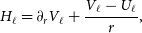 \begin{equation}H_{\ell}=\partial_{r}V_{\ell}+\frac{V_{\ell}-U_{\ell}}{r},\,\end{equation}
 \begin{equation}\chi_{\ell}=\partial_{r}U_{\ell}+\frac{2}{r}U_{\ell}-\frac{\ell\left(\ell+1\right)}{r}V_{\ell}.\end{equation}
In particular, the scalar functions  $\chi_\ell$ are related to the relative volume change $\Delta$ via an expansion in Legendre polynomials as
 \begin{equation}\Delta = \boldsymbol{\nabla\cdot {\boldsymbol{u}}}=\sum_{\ell=0}^{\infty}\chi_{\ell}P_{\ell}.\end{equation}
According to the incompressibility assumptions, there are no volume changes  $\Delta$ in our model. However, during the deformations, also incompressible materials must be able to react to isotropic stresses. We thus require that the bulk modulus $\kappa$ is infinitely large but in such a way that the material increment of the pressure, which can be expressed as $p^\delta=-\kappa \Delta$, remains finite (Sabadini et al. Reference Sabadini, Vermeersen and Cambiotti2016). Therefore, the coefficients $p_{\ell}$ of the expansion in spherical harmonics of $p^\delta$ remain finite when the formal limit
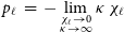 \begin{equation*} p_{\ell} = - \lim_{ \substack{\chi_{\ell}\to 0 \\ \kappa \to \infty }}\kappa \, \chi_{\ell}\, \end{equation*}
is taken (Love Reference Love1959). Using the incompressibility assumption  $\chi_{\ell}=0$ into equation (30) gives a relation between the radial and the tangential displacements:
 \begin{equation} V_{\ell}=\frac{r\partial_{r}U_{\ell}+2U_{\ell}}{\ell \left(\ell +1\right)} .\end{equation}
The quantity  $H_{\ell}$ can thus be written as
 \begin{equation}H_{\ell}=\frac{\nabla_{r}^{2}\left(U_{\ell }r\right)}{\ell\left(\ell+1\right)}.\end{equation}
Since, in our model, the layers are homogeneous (i.e.  $\partial_{r}\rho_{0}=0$), equation (28) within each layers becomes the Laplace equation ( $\ell\geq1$)
 \begin{equation}\nabla_{r}^{2}\Phi_{\ell}=0 .\end{equation}
As usual, we write the solution of equation (34) as
 \begin{equation}\Phi_{\ell} = c_3 r^{\ell} + c_3^*r^{-\left(\ell+1\right)} ,\end{equation}
where  $c_3$ and $c_3^*$ are constants of integration. We underline that the absence of density perturbations within the layers does not implies that the gravitational perturbation $\Phi^{\Delta}$ is zero. Indeed, there are density jumps $\Delta\rho_{\lambda}$ between different layers at interfaces defined by $r=\lambda$,
 \begin{equation}\Delta\rho_{\lambda}=\rho_{0}\left(\lambda^{+}\right)-\rho_{0}\left(\lambda^{-}\right).\end{equation}
This means that we can write the density gradient as
 \begin{equation*}\partial_{r}\rho_{0}=(\rho_{c}-\rho_{f})\delta(r-R'),\end{equation*}
 \begin{equation*}\partial_{r}\rho_{0}=-\rho_{c}\delta(r-R),\end{equation*}
at the interfaces  $r=R'$ and $r=R$, respectively.
The introduction of the auxiliary quantity,
 \begin{equation*}\Gamma_{\ell} = -\frac{p_{\ell}}{\rho_{0}}-gU_{\ell}-\Phi_{\ell}, \end{equation*}
allows us to reduce equations (26) and (27) to
 \begin{equation}\partial_{r}\Gamma_{\ell}+\frac{\mu}{\rho_{0}}\frac{\ell\left(\ell+1\right)}{r}H_{\ell} =0,\end{equation}
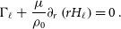 \begin{equation}\Gamma_{\ell}+\frac{\mu}{\rho_{0}}\partial_{r}\left(rH_{\ell}\right)=0.\end{equation}
These two equations can be combined into
 \begin{equation}\nabla_{r}^{2} \, \Gamma_{\ell}=0,\end{equation}
which has the solution
 \begin{equation}\Gamma_{\ell}=-\frac{\mu}{\rho_{0}} \, c_{1} \,r^{\ell} - \frac{\mu}{\rho_{0}} \, c_{1}^{*} \, r^{-\ell-1},\end{equation}
where the quantity  $\mu/\rho_{0}$ have been inserted for convenience and $c_1$, $c_1^*$ are two constants. Inserting this solution in (37) and using the relation (33), we obtain a differential equation for $U_{\ell}$:
 \begin{equation}\nabla_{r}^{2} ( U_{\ell} \, r ) = c_{1} \, \ell \, r^{\ell} - c_{1}^{*} \,(\ell+1) \, r^{-\ell-1}. \end{equation}
Solving this equation and using (32), we finally get the radial and tangential displacements as
 \begin{equation}U_{\ell} = c_{1}\frac{\ell\:r^{\ell+1}}{2\left(2\ell+3\right)}+c_{2}r^{\ell-1}+ c_{1}^*\frac{\left(\ell+1\right)r^{-\ell}}{2\left(2\ell-1\right)}+c_{2}^*r^{-\left(\ell+2\right)}, \end{equation}
 $$\eqalign{l{V_\ell } = {c_1}{{\left( {\ell + 3} \right){r^{\ell + 1}}} \over {2\left( {2\ell + 3} \right)\left( {\ell + 1} \right)}} + {c_2}{{{r^{\ell - 1}}} \over \ell } + . & .. \cr & ... + c_1^*{{\left( {2 - \ell } \right){r^{ - \ell }}} \over {2l\left( {2\ell - 1} \right)}} - c_2^*{{{r^{ - \left( {\ell + 2} \right)}}} \over {\ell + 1}}. \cr} $$
We remind that the centrifugal potential can be expanded in Legendre polynomials as
 \begin{equation} \phi^{C}\left(r,\theta,\varphi\right) = \phi_{0}^{C}\left(r\right)P_{0}\left(\theta\right)+\phi_{2}^{C}\left(r\right)P_{2}\left(\theta\right) ,\end{equation}
where
 \begin{equation}\phi_{0}^{C}\left(r\right)=-\frac{\Omega^{2}r^{2}}{3},\end{equation}
and
 \begin{equation} \phi_{2}^{C}\left(r\right) = \frac{\Omega^{2}r^{2}}{3}.\end{equation}
All the harmonic coefficients with  $\ell \neq 0, 2 $ are zero. Moreover, the coefficient with $\ell=0$ is suppressed by the request of incompressibility. Therefore, in the case of deformations induced by the centrifugal force, we have only the harmonic contribution corresponding to $\ell=2$. In this, scenario is easy to see that the above expression for the radial and tangential displacement (42) and (43) have the same form of the ones given in equation (7). Note that, differently from the FLE model, where there are only four constants (a, A, b and B), now six coefficients need to be determined ( $c_1$, $c_2$, $c_1^*$, $c_2^*$, $c_3$, $c_3^*$): two new coefficients come from the self-consistent treatment of the Poisson equation and have been introduced in equation (35). In order to fix these constants, we have to impose the opportune boundary conditions at the interface between layers.
A.1. Boundary conditions
The boundary condition can be easily written by using the expansion in spherical harmonics of the material incremental stress, that is,
 \begin{equation}\boldsymbol{\sigma}\cdot{\boldsymbol{e}}_{r}=\sum_{\ell}\left(R_{\ell}P_{\ell}{\boldsymbol{e}}_{r}+S_{\ell}\partial_{\theta}P_{\ell}{\boldsymbol{e}}_{\theta}\right),\end{equation}
where  ${\boldsymbol{e}}_{r}$ and ${\boldsymbol{e}}_{\theta}$ are the usual spherical unit vector. We call $R_{\ell}$ and $S_{\ell}$ radial and tangential stress, respectively. We require the continuity of the radial stress and that the tangential stress must be zero both at the star’s surface $r=R$ and at the core–crust boundary $r=R'$:
 \begin{align} R_{\ell}(R^{+})\,& = 0,\end{align}
 \begin{align} R_{\ell}(R^{+})\,& =R_{\ell}(R'^{-}),\end{align}
 \begin{align} S_{\ell}(R^{+}) \,& = 0,\end{align}
 \begin{align}
S_{\ell}(R'^{+}) & = 0.\end{align}
\begin{align}
S_{\ell}(R'^{+}) & = 0.\end{align}
In fact, the fluid core and the vacuum outside the star cannot support shear stress; moreover, pressure is zero for  $r\geq R$. We can add other two conditions for the potential, by introducing the potential stress
 \begin{equation}Q_{\ell} = \partial_{r}\Phi_{\ell}+\frac{\ell+1}{r}\Phi_{\ell}+4\pi G\rho_{0}U_{\ell} .\end{equation}
Starting from the Poisson equation (23) and using the Gauss theorem in a pillow box placed at a radius  $r=R$ and $r=R'$, respectively, we can write the boundary conditions in a compact form:
 \begin{align} Q_{\ell}(R^{+})\,& =\,Q_{\ell}(R^{-}),\end{align}
 \begin{align} Q_{\ell}(R'^{+})\,& =\,Q_{\ell}(R'^{-}).\end{align}
In particular, using the spherical harmonic expansion (44) of the centrifugal potential
 \begin{equation}\Phi_{\ell}^{C}\left(r\right)=\Phi_{\ell}^{C}\left(R\right)\left(\frac{r}{R}\right)^{\ell},\,\,\ell > 0,\end{equation}
equation (53) can be explicitly written as
 $$\displaylines{{\partial _r}{\Phi _\ell }\left( {{R^ - }} \right) + {{\ell + 1} \over r}{\Phi _\ell }\left( {{R^ - }} \right) + 4\pi G{\rho _0}\left( {{R^ - }} \right){U_\ell }\left( {{R^ - }} \right) = \cr = {{2\ell + 1} \over {{R^ + }}}\Phi _\ell ^C\left( {{R^ + }} \right).} $$
The six boundary conditions [(48), (50), (53), (49), (51), and (54)] fix the coefficients, giving us the analytical displacements, stresses, and potential.
Appendix B. Coefficients
In this appendix, we show the explicit form of the displacement coefficients, both for the FLE model in the Cowling approximation and for our two-density model. We recall here the main physical quantities of the problem: R is the stellar radius, R´ the core–crust interface radius,  $c_t=\sqrt{\mu/\rho_c}$ is the transverse speed of shear waves, and $v_K=\sqrt{GM/R}$ is the Keplerian velocity. We also recall the definition of three useful dimensionless parameters that have been used in the text: $\chi=c_t/v_K$, $d=\rho_c/\rho_f<1$, and $q=1-L$. Since $q\ll 1$, we expand the coefficients $\skew4\tilde{a}$, $\skew2\tilde{b}$, $\skew2\tilde{A}$, $\skew4\tilde{B}$, and Q up to the second order in q.
B.1. Cowling approximation
The displacement in equation (7) can be rearranged in the form (9). If we use the Cowling approximation, discussed in Section 3.2, we have different parameters with respect to the FLE case:
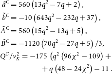 \begin{align}\begin{split}\skew4\tilde{a}^C & =560 \left(13 q^2-7 q+2\right),\\ \skew2\tilde{b}^C & =-10 \left(643 q^2-232 q+37\right),\\ \skew2\tilde{A}^C & =560 \left(15 q^2-13 q+5\right),\\ \skew4\tilde{B}^C & = - 1120 \left( 70 q^2 - 27 q + 5 \right) / 3, \\ Q^C & / v_K^2 =-175 \, \left( q^2 \left( 96 \chi^2 - 109 \right)\right. + \\ & \qquad \qquad + q \left( 48 - 24 \chi^2 \right) - 11. \end{split}\end{align}
It is now easy to check that equation (16) is valid when the (very small) terms proportional to  $q^2 \chi^2$ and $q \chi^2$ are neglected.
B.2. Two-density model
As discussed in Section 4, the displacements for the two-density model have the same analytic form given in equation (9). In this case, the coefficients which appear into the explicit solution of the displacements are given by
 \begin{align*}\skew4\tilde{a} = &q^2 (-1\,680 d^3 v^2+8\,400 d^2 v^2-33\,600 d v^2 \chi ^2+ \\ & -6\,720 d v^2+44\,520 v^2 \chi ^2)+ \\ & +q (-840 d^2 v^2+6\,720 d v^2 \chi ^2+ \\ & +840 d v^2-12\,600 v^2 \chi ^2)+ \\ & +1\,680 v^2 \chi^2, \end{align*}
 \begin{align*}\skew2\tilde{b} = & q^2 \left(405 d^3 v^2-1\,575 d^2 v^2+14\,400 d v^2 \chi ^2+\right. \\ & \left.+1\,170 d v^2-24\,045 v^2 \chi ^2\right)+ \\ & +q \left(90 d^2 v^2-1\,920 d v^2 \chi ^2-90 d v^2+5\,400 v^2 \chi ^2\right)+ \\ & -555 v^2 \chi ^2,\end{align*}
 \begin{align*}\skew2\tilde{A} = & q^2 (-3\,780 d^3 v^2+15\,435 d^2 v^2-63\,840 d v^2 \chi ^2+ \\ & -11\,655 d v^2+76\,440 v^2 \chi ^2)+ \\ & q (-1\,575 d^2 v^2+15\,960 d v^2 \chi ^2+ \\ & +1\,575 d v^2-26\,880 v^2 \chi ^2) + \\ & 4\,200 v^2 \chi ^2,\end{align*}
 \begin{align*}\skew4\tilde{B} = & q^2 \left(58\,240 d v^2 \chi ^2+1\,680 (d-1)^2 d v^2-97\,440 v^2 \chi ^2\right)+ \\ & q \left(24\,080 v^2 \chi ^2-8\,960 d v^2 \chi ^2\right) + \\ & -2\,800 v^2 \chi ^2,\end{align*}
 \begin{align*}Q/v_K^2 = & q^2 (1\,890 d^3 v^2-8\,820 d^2 v^2 \chi ^2-7\,560 d^2 v^2+ \\ & +35\,070 d v^2 \chi ^2+ \\ & +5\,670 d v^2+50\,400 v^2 \chi ^4-49\,140 v^2 \chi ^2)+ \\ & q (630 d^2 v^2-5\,250 d v^2 \chi ^2-630 d v^2-12\,600 v^2 \chi ^4+ \\ & +15\,330 v^2 \chi ^2)+ \\ & -2\,310 v^2 \chi ^2 .\end{align*}
The exact form of these coefficients is much more complex; here expressions have been truncated to the second order in q, which is the relative crust thickness.



