


1. Introduction
Networks are a simple model for complex relationships with entities or objects represented as nodes and their interactions or relationships encoded as edges. One observed feature in many networks is core-periphery (CP) structure, where nodes form two distinct groups: a densely-connected core and a sparsely-connected periphery (Csermely et al. Reference Csermely, London, Wu and Uzzi2013; Yanchenko and Sengupta Reference Yanchenko and Sengupta2023). While there is not a universal definition, CP structure is distinct from the more well-known assortative mixing in that the core and periphery are densely and sparsely connected, respectively, and there is greater density between core and peripheral nodes than within the periphery itself. CP structure has been observed across many domains including: airport networks (Lordan and Sallan Reference Lordan and Sallan2017, Reference Lordan and Sallan2019), power grid networks (Yang et al. Reference Yang, Huang, Hu, Cheng, Pei and Li2021), economic networks (Krugman Reference Krugman1996; Magone et al. Reference Magone, Laffan and Schweiger2016), and more. We refer the interested reader to (Yanchenko and Sengupta Reference Yanchenko and Sengupta2023) for a more thorough review.
One of the most popular approaches to detect and quantify CP structure is the Borgatti and Everett (BE) metric which finds the correlation between the observed network and an “ideal” CP structure (Borgatti and Everett Reference Borgatti and Everett2000). Here, we focus on the discrete model where nodes are assigned exclusively to either the core or periphery. There are multiple implementations available for this method, including the UCInet software (Borgatti et al. Reference Borgatti, Everett and Freeman2002) and cpnet Python package. But as networks continue to increase in size, it is important for applied researchers to have efficient algorithms to quickly and accurately detect this CP structure.
In this work, we detail a greedy, label-switching algorithm to identify CP structure in networks. Our first contribution is to thoroughly benchmark an existing algorithm (Yanchenko Reference Yanchenko2022), demonstrating that it yields more accurate CP labels compared to a competing implementation. Moreover, we prove that this algorithm enjoys both monotone ascent and finite termination at a local optimum, and, on small networks, typically yields objection function values within 90% of the global optimum. The other major contribution is a computational improvement to the algorithm in Yanchenko (Reference Yanchenko2022), introducing an incremental-update implementation which significantly improves speed and scalability. Specifically, we exploit a mathematical reformulation of the BE metric which yields an order-of-magnitude speed-up compared to a naive algorithm. Empirical results show the algorithm to be significantly faster than both a naive implementation and competing method, and on one- real-world network (DBLP (Gao et al. Reference Gao, Liang, Fan, Sun and Han2009; Ji et al. Reference Ji, Sun, Danilevsky, Han and Gao2010)), it is 340 times faster.
In related work, there have been several notable developments in fast algorithms for statistical network analysis, particularly for community detection, model fitting, and two-sample testing. Amini et al. (Reference Amini, Chen, Bickel and Levina2013) proposed a fast pseudo-likelihood method for community detection, which was subsequently refined by Wang et al. (Reference Wang, Zhang, Liu, Zhu and Guo2023). Zhang et al. (Reference Zhang, Song, Lu and Zhu2023) introduced a distributed algorithm for large-scale block models with a grouped community structure. Divide-and-conquer strategies have also gained attention as scalable alternatives to global community detection in large networks (Chakrabarty et al. Reference Chakrabarty, Sengupta and Chen2025b; Mukherjee et al. Reference Mukherjee, Sarkar and Bickel2021; Wu et al. Reference Wu, Li and Zhu2020). More recently, subsampling-based approaches have been developed for computationally efficient network analysis. Bhadra et al. (Reference Bhadra, Pensky and Sengupta2025) proposed a predictive subsampling method for fast community detection, while Chakraborty et al. (Reference Chakraborty, Sengupta and Chen2025c) introduced a subsampling-based framework for scalable estimation and two-sample testing. In parallel, Chakrabarty et al. (Reference Chakrabarty, Sengupta and Chen2025a) developed a subsampling-based approach for network cross-validation and model selection. Lastly, Yanchenko (Reference Yanchenko2022) and Yanchenko (Reference Yanchenko2025) develop divide-and-conquer algorithms for fast CP identification in large networks. Here, we leverage the base algorithm of these works and further detail the computational improvements.
The remainder of this paper is organized as follows. In Section 2, we describe the BE metric while in Section 3 we detail a computationally efficient algorithm and examine some of its properties. Experiments on simulated and real-world networks are the subjects of Sections 4 and 5, respectively, and we share concluding thoughts in Section 6.
2. Core-periphery metric
Consider a network with
 $n$
nodes and let
$n$
nodes and let
 $\textbf {A}$
be the corresponding
$\textbf {A}$
be the corresponding
 $n\times n$
adjacency matrix where
$n\times n$
adjacency matrix where
 $A_{ij}=1$
if nodes
$A_{ij}=1$
if nodes
 $i$
and
$i$
and
 $j$
have an edge, and 0 otherwise, and
$j$
have an edge, and 0 otherwise, and
 $A_{ij}\mid P_{ij}\stackrel {\text{ind.}}{\sim }\mathsf{Bernoulli}(P_{ij})$
for
$A_{ij}\mid P_{ij}\stackrel {\text{ind.}}{\sim }\mathsf{Bernoulli}(P_{ij})$
for
 $0\leq i\lt j\leq n$
. We write
$0\leq i\lt j\leq n$
. We write
 ${\textbf {A}}\sim \textbf {P}$
as shorthand for this model. For simplicity, we only consider unweighted, undirected networks with no self-loops. We also define
${\textbf {A}}\sim \textbf {P}$
as shorthand for this model. For simplicity, we only consider unweighted, undirected networks with no self-loops. We also define
 $\boldsymbol c\in \{0,1\}^n$
as the CP assignment vector where
$\boldsymbol c\in \{0,1\}^n$
as the CP assignment vector where
 $c_i=1$
if node
$c_i=1$
if node
 $i$
is assigned to the core, and 0 if assigned to the periphery where
$i$
is assigned to the core, and 0 if assigned to the periphery where
 $k=\sum _{i=1}^n c_i$
is the size of the core. For a given
$k=\sum _{i=1}^n c_i$
is the size of the core. For a given
 $\boldsymbol c$
, let
$\boldsymbol c$
, let
 $\Delta (\boldsymbol c)\equiv \Delta$
be an
$\Delta (\boldsymbol c)\equiv \Delta$
be an
 $n\times n$
matrix such that
$n\times n$
matrix such that
 $\Delta _{ij}=c_i+c_j - c_ic_j$
, i.e.,
$\Delta _{ij}=c_i+c_j - c_ic_j$
, i.e.,
 $\Delta _{ij}=1$
if node
$\Delta _{ij}=1$
if node
 $i$
or
$i$
or
 $j$
is assigned to the core, and 0 otherwise. Then
$j$
is assigned to the core, and 0 otherwise. Then
 $\Delta$
represents an “ideal” CP structure where each core node is connected to all other nodes, each periphery node is connected to all core nodes, but periphery nodes have no connections among themselves. The notion of ideal CP structure can be generalized such that
$\Delta$
represents an “ideal” CP structure where each core node is connected to all other nodes, each periphery node is connected to all core nodes, but periphery nodes have no connections among themselves. The notion of ideal CP structure can be generalized such that
 $\Delta _{ij}\in (0,1)$
or
$\Delta _{ij}\in (0,1)$
or
 $\Delta _{ij}=N/A$
when one node is in the core and the other in the periphery (Borgatti and Everett Reference Borgatti and Everett2000).
$\Delta _{ij}=N/A$
when one node is in the core and the other in the periphery (Borgatti and Everett Reference Borgatti and Everett2000).
Although there are many possible definitions of CP structure, Borgatti and Everett (Reference Borgatti and Everett2000) quantify the property by defining:
 \begin{equation} T({\textbf {A}},\boldsymbol c) =\mathsf{Cor}({\textbf {A}},\Delta ), \end{equation}
i.e., the Pearson correlation between the upper-triangles of
 $\textbf {A}$
and
$\textbf {A}$
and
 $\Delta$
. We can rewrite (1) as
$\Delta$
. We can rewrite (1) as
 \begin{align} T({\textbf {A}},\boldsymbol c) &=\frac {\sum _{i\lt j}(A_{ij}-\bar A)(\Delta _{ij}-\bar \Delta )}{\frac 12n(n-1)\{\bar A(1-\bar A)\bar \Delta (1-\bar \Delta )\}^{1/2}}\notag \\ &=\frac {\sum _{i\lt j}A_{ij}\Delta _{ij}-\frac 12n(n-1)\bar A\bar \Delta }{\frac 12n(n-1)\{\bar A(1-\bar A)\bar \Delta (1-\bar \Delta )\}^{1/2}} \end{align}
where
 $\bar X$
is the entry-wise mean of the upper-triangle of matrix
$\bar X$
is the entry-wise mean of the upper-triangle of matrix
 $X$
. For a recent extension of this metric, please see Estévez and Nordlund (Reference Estévez and Nordlund2025). The form in (2) is more amenable to statistical analysis and will be leveraged in the remainder of this work. Lastly, the labels
$X$
. For a recent extension of this metric, please see Estévez and Nordlund (Reference Estévez and Nordlund2025). The form in (2) is more amenable to statistical analysis and will be leveraged in the remainder of this work. Lastly, the labels
 $\boldsymbol c$
are typically unknown so we must find the optimal labels, i.e.,
$\boldsymbol c$
are typically unknown so we must find the optimal labels, i.e.,
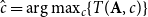
 \begin{equation} \hat {\boldsymbol{c}} =\arg \max _{\boldsymbol c}\{T({\textbf {A}},\boldsymbol c)\}. \end{equation}
The space of all possible solutions,
 $\{0,1\}^n$
, has
$\{0,1\}^n$
, has
 $\mathcal O(e^n)$
elements, meaning that an exhaustive search to find the globally optimal solution is not feasible for even moderately sized networks. Thus, an optimization algorithm must be employed to find an approximation of the global optimum. The remainder of this paper is devoted to such an algorithm that is both computationally efficient and empirically accurate.
$\mathcal O(e^n)$
elements, meaning that an exhaustive search to find the globally optimal solution is not feasible for even moderately sized networks. Thus, an optimization algorithm must be employed to find an approximation of the global optimum. The remainder of this paper is devoted to such an algorithm that is both computationally efficient and empirically accurate.
3. Algorithm
3.1. Label-switching algorithm
We first detail an efficient algorithm to approximate
 $\hat {\boldsymbol{c}}$
in (3), building off that of Yanchenko (Reference Yanchenko2022). While both Yanchenko (Reference Yanchenko2022) and Yanchenko (Reference Yanchenko2025) employ divide-and-conquer methods, our focus is working directly with the entire network, though the following algorithm can easily be integrated into these approaches. After randomly initializing the CP labels, one at a time and for each node
$\hat {\boldsymbol{c}}$
in (3), building off that of Yanchenko (Reference Yanchenko2022). While both Yanchenko (Reference Yanchenko2022) and Yanchenko (Reference Yanchenko2025) employ divide-and-conquer methods, our focus is working directly with the entire network, though the following algorithm can easily be integrated into these approaches. After randomly initializing the CP labels, one at a time and for each node
 $i$
, we swap the label of the node and compute (2) with these new labels. The new label is kept if the objective function value is (strictly) larger than before, otherwise the original label remains. This process repeats until the labels are unchanged for an entire cycle through all
$i$
, we swap the label of the node and compute (2) with these new labels. The new label is kept if the objective function value is (strictly) larger than before, otherwise the original label remains. This process repeats until the labels are unchanged for an entire cycle through all
 $n$
nodes. Our approach is similar to the Kernighan-Lin algorithm for graph partitioning (Kernighan and Lin Reference Kernighan and Lin1970) since both perform greedy, local searches. Unlike our algorithm, however, the group sizes are fixed in the Kernighan-Lin algorithm. The proposed approach is detailed in Algorithm 1.
$n$
nodes. Our approach is similar to the Kernighan-Lin algorithm for graph partitioning (Kernighan and Lin Reference Kernighan and Lin1970) since both perform greedy, local searches. Unlike our algorithm, however, the group sizes are fixed in the Kernighan-Lin algorithm. The proposed approach is detailed in Algorithm 1.
3.2. Computational improvement
The main computational bottleneck in Algorithm 1 comes from computing
 $T({\textbf {A}},\boldsymbol c')$
. Ostensibly, this requires
$T({\textbf {A}},\boldsymbol c')$
. Ostensibly, this requires
 $\mathcal O(n^2)$
operations since we must compute
$\mathcal O(n^2)$
operations since we must compute
 $M(\boldsymbol c)=\sum _{i\lt j}A_{ij}\Delta _{ij}(\boldsymbol c)$
and
$M(\boldsymbol c)=\sum _{i\lt j}A_{ij}\Delta _{ij}(\boldsymbol c)$
and
 $\bar A=\sum _{i\lt j}A_{ij}/\{\frac 12n(n-1)\}$
. We call such an implementation greedyNaive. We can leverage the reformulation of the BE metric from (2), however, to improve the computational efficiency of Algorithm 1 from that of the original algorithm in Yanchenko (Reference Yanchenko2022). The following is a similar idea to that of Kojaku and Masuda (Reference Kojaku and Masuda2017). In particular,
$\bar A=\sum _{i\lt j}A_{ij}/\{\frac 12n(n-1)\}$
. We call such an implementation greedyNaive. We can leverage the reformulation of the BE metric from (2), however, to improve the computational efficiency of Algorithm 1 from that of the original algorithm in Yanchenko (Reference Yanchenko2022). The following is a similar idea to that of Kojaku and Masuda (Reference Kojaku and Masuda2017). In particular,
 $T({\textbf {A}},\boldsymbol c')$
can be efficiently updated since
$T({\textbf {A}},\boldsymbol c')$
can be efficiently updated since
 $\boldsymbol c'$
differs from the current CP labels by only a single entry. While the following approach has been used in previous works (e.g., Yanchenko Reference Yanchenko2025), the details of this computational improvement have yet to be formally described and thoroughly investigated.
$\boldsymbol c'$
differs from the current CP labels by only a single entry. While the following approach has been used in previous works (e.g., Yanchenko Reference Yanchenko2025), the details of this computational improvement have yet to be formally described and thoroughly investigated.
Label-switching for CP detection

We call the following approach greedyFast. At initialization, there are no shortcuts and the objective function
 $T({\textbf {A}},\boldsymbol c)$
must be computed as in (2), which takes
$T({\textbf {A}},\boldsymbol c)$
must be computed as in (2), which takes
 $\mathcal O(n^2)$
operations. Now, let
$\mathcal O(n^2)$
operations. Now, let
 $(\boldsymbol c')^{(i)}$
be the proposed CP labels where
$(\boldsymbol c')^{(i)}$
be the proposed CP labels where
 $(c')_i^{(i)}=1-c_i$
and
$(c')_i^{(i)}=1-c_i$
and
 $(c')_j^{(i)}=c_j$
for
$(c')_j^{(i)}=c_j$
for
 $j\neq i$
, i.e., the labels differ only at node
$j\neq i$
, i.e., the labels differ only at node
 $i$
. It is clear that we only need to update
$i$
. It is clear that we only need to update
 $\bar \Delta$
and
$\bar \Delta$
and
 $M(\boldsymbol c)$
to compute
$M(\boldsymbol c)$
to compute
 $T({\textbf {A}},(\boldsymbol c')^{(i)})$
. We know that
$T({\textbf {A}},(\boldsymbol c')^{(i)})$
. We know that
 $\bar \Delta (\boldsymbol c)=\{\frac 12k(k-1)+k(n-k)\}/\{\frac 12n(n-1)\}$
where
$\bar \Delta (\boldsymbol c)=\{\frac 12k(k-1)+k(n-k)\}/\{\frac 12n(n-1)\}$
where
 $k=\sum _{j=1}^n c_j$
. If
$k=\sum _{j=1}^n c_j$
. If
 $k'$
is the size of the core for labels
$k'$
is the size of the core for labels
 $(\boldsymbol c')^{(i)}$
, then
$(\boldsymbol c')^{(i)}$
, then
 $k'=k+1$
if
$k'=k+1$
if
 $c_i=0$
, and
$c_i=0$
, and
 $k'=k-1$
if
$k'=k-1$
if
 $c_i=1$
. Thus
$c_i=1$
. Thus
 $\bar \Delta ((\boldsymbol c')^{(i)})=\{\frac 12k'(k'-1)+k'(n-k')\}/\{\frac 12n(n-1)\}$
can be computed in
$\bar \Delta ((\boldsymbol c')^{(i)})=\{\frac 12k'(k'-1)+k'(n-k')\}/\{\frac 12n(n-1)\}$
can be computed in
 $\mathcal O(1)$
. The key step is computing
$\mathcal O(1)$
. The key step is computing
 $M((\boldsymbol c')^{(i)})$
by using
$M((\boldsymbol c')^{(i)})$
by using
 $M(\boldsymbol c)$
. Notice that
$M(\boldsymbol c)$
. Notice that
 \begin{align} M((\boldsymbol c')^{(i)}) &=\sum _{j=1}^n\sum _{k=1}^{j-1} A_{jk}\Delta _{jk}((\boldsymbol c')^{(i)}) \\ \notag &=\sum _{j\neq i}^n\sum _{k=1}^{j-1}A_{jk}\Delta _{ik}((\boldsymbol c')^{(i)}) +\sum _{k=1}^{i-1} A_{ik}\Delta _{ik}((\boldsymbol c')^{(i)})\\ \notag &=\sum _{j\neq i}^n\sum _{k=1}^{j-1}A_{jk}\Delta _{jk}(\boldsymbol c) +\sum _{k=1}^{i-1} A_{ik}\Delta _{ik}((\boldsymbol c')^{(i)})\\ \notag &= \left (M(\boldsymbol c) -\sum _{k=1}^{i-1} A_{ik}\Delta _{ik}(\boldsymbol c)\right ) +\sum _{k=1}^{i-1} A_{ik}\Delta _{ik}((\boldsymbol c')^{(i)})\\ \notag &=M(\boldsymbol c)+\sum _{k=1}^{i-1}A_{ik}\{\Delta _{ik}((\boldsymbol c')^{(i)})-\Delta _{ik}(\boldsymbol c)\}. \end{align}
Since we have already computed
 $M(\boldsymbol c)$
, the only term we need to compute in (4) is the final sum, which requires
$M(\boldsymbol c)$
, the only term we need to compute in (4) is the final sum, which requires
 $\mathcal O(n)$
operations. Thus, while the initial evaluation of
$\mathcal O(n)$
operations. Thus, while the initial evaluation of
 $T({\textbf {A}},\boldsymbol c)$
is
$T({\textbf {A}},\boldsymbol c)$
is
 $\mathcal O(n^2)$
, we can update its value in
$\mathcal O(n^2)$
, we can update its value in
 $\mathcal O(n)$
. In Section 6, we discuss how this could be improved even further using an edge list instead of adjacency matrix. Additionally, this type of improvement could also be used to efficiently calculate alternative CP objective functions, i.e., Equation. (4) in Borgatti and Everett (Reference Borgatti and Everett2000) where the number of CP edges are excluded and only core-core and periphery-periphery edges are used.
$\mathcal O(n)$
. In Section 6, we discuss how this could be improved even further using an edge list instead of adjacency matrix. Additionally, this type of improvement could also be used to efficiently calculate alternative CP objective functions, i.e., Equation. (4) in Borgatti and Everett (Reference Borgatti and Everett2000) where the number of CP edges are excluded and only core-core and periphery-periphery edges are used.
3.3. Time complexity
We precisely characterize the complexity of one pass of the modified algorithm. Since there are
 $n$
nodes in the network, initializing the CP labels is
$n$
nodes in the network, initializing the CP labels is
 $\mathcal O(n)$
, as is randomly ordering the nodes. Computing
$\mathcal O(n)$
, as is randomly ordering the nodes. Computing
 $T({\textbf {A}},\boldsymbol c)$
is
$T({\textbf {A}},\boldsymbol c)$
is
 $\mathcal O(n^2)$
, but
$\mathcal O(n^2)$
, but
 $T({\textbf {A}},\boldsymbol c')$
can be updated with only
$T({\textbf {A}},\boldsymbol c')$
can be updated with only
 $\mathcal O(n)$
operations. This must be computed for each node such that one pass of the for loop takes
$\mathcal O(n)$
operations. This must be computed for each node such that one pass of the for loop takes
 $\mathcal O(n^2)$
operations. Note that if we re-computed
$\mathcal O(n^2)$
operations. Note that if we re-computed
 $T({\textbf {A}},\boldsymbol c')$
from scratch at every iteration, then the pass would require
$T({\textbf {A}},\boldsymbol c')$
from scratch at every iteration, then the pass would require
 $\mathcal O(n^3)$
operations. Thus, our improvement yields an order-of-magnitude computational speed-up.
$\mathcal O(n^3)$
operations. Thus, our improvement yields an order-of-magnitude computational speed-up.
3.4. Convergence guarantees
In this sub-section, we discuss some of the theoretical properties of the proposed algorithm. Algorithm 1 is a greedy algorithm in the sense that it makes the locally optimal decision. Ideally, we hope that this algorithm adequately approximates the global optimum in (3).
We first establish monotone ascent to a local maximum for Algorithm 1. To do so, we first must define what “local” means. Let
 $N(\boldsymbol c)$
be a neighborhood of label
$N(\boldsymbol c)$
be a neighborhood of label
 $\boldsymbol c$
defined as
$\boldsymbol c$
defined as
 \begin{equation*} N(\boldsymbol c) =\left \{\boldsymbol c':\sum _{i=1}^n\mathbb I(c_i'\neq c_i)=1\right \}. \end{equation*}
where
 $\mathbb I(\!\cdot \!)$
is the indicator function. In words, this is the set of all CP labels that differ from
$\mathbb I(\!\cdot \!)$
is the indicator function. In words, this is the set of all CP labels that differ from
 $\boldsymbol c$
by only one node assignment. In the following proposition, we show that Algorithm 1 converges to a local optimum by this definition.
$\boldsymbol c$
by only one node assignment. In the following proposition, we show that Algorithm 1 converges to a local optimum by this definition.
Proposition 1.
Let
 $\hat {\boldsymbol{c}}_1$
be the labels returned by Algorithm 1. Then for all
$\hat {\boldsymbol{c}}_1$
be the labels returned by Algorithm 1. Then for all
 $\boldsymbol c\in N(\hat {\boldsymbol{c}}_1)$
,
$\boldsymbol c\in N(\hat {\boldsymbol{c}}_1)$
,
 $T({\textbf {A}},\hat {\boldsymbol{c}}_1)\geq T({\textbf {A}},\boldsymbol c)$
, i.e., Algorithm 1 enjoys monotone ascent to a local maximum.
$T({\textbf {A}},\hat {\boldsymbol{c}}_1)\geq T({\textbf {A}},\boldsymbol c)$
, i.e., Algorithm 1 enjoys monotone ascent to a local maximum.
A brief proof is given in Appendix A. We emphasize that since Algorithm 1 updates the labels only when
 $T({\textbf {A}},\boldsymbol c')$
is strictly greater than
$T({\textbf {A}},\boldsymbol c')$
is strictly greater than
 $T({\textbf {A}},\boldsymbol c)$
, cycling among equal-valued CP labels cannot occur. Proposition 1 ensures that the labels returned by Algorithm 1 yield a local maximum of
$T({\textbf {A}},\boldsymbol c)$
, cycling among equal-valued CP labels cannot occur. Proposition 1 ensures that the labels returned by Algorithm 1 yield a local maximum of
 $T({\textbf {A}},\boldsymbol c)$
. We would like to have some guarantee, however, of how close this result is to the global maximum. In many proofs that an algorithm achieves the global maximum, the sub-modularity of the objective function is required, e.g., Kempe et al. (Reference Kempe, Kleinberg and Tardos2003). Unfortunately, the BE metric is not sub-modular, meaning that there are no greedy optimality guarantees, and we can only prove the monotone ascent property of Proposition 1.
$T({\textbf {A}},\boldsymbol c)$
. We would like to have some guarantee, however, of how close this result is to the global maximum. In many proofs that an algorithm achieves the global maximum, the sub-modularity of the objective function is required, e.g., Kempe et al. (Reference Kempe, Kleinberg and Tardos2003). Unfortunately, the BE metric is not sub-modular, meaning that there are no greedy optimality guarantees, and we can only prove the monotone ascent property of Proposition 1.
For small
 $n$
, however, we can empirically compare Algorithm 1 to the global optimum by using a brute-force approach. Specifically, we let
$n$
, however, we can empirically compare Algorithm 1 to the global optimum by using a brute-force approach. Specifically, we let
 $n=20$
and generate Erdos-Renyi (ER) networks with
$n=20$
and generate Erdos-Renyi (ER) networks with
 $P_{ij}=p$
for all
$P_{ij}=p$
for all
 $i,j$
(Erdös and Rényi Reference Erdös and Rényi1959). We use ER networks because they do not have an intrinsic CP structure, making the optimization task more difficult. Since
$i,j$
(Erdös and Rényi Reference Erdös and Rényi1959). We use ER networks because they do not have an intrinsic CP structure, making the optimization task more difficult. Since
 $n=20$
, there are
$n=20$
, there are
 $2^{20}\approx 10^6$
possible CP labels and we evaluate each one (exhaustive enumeration) to find
$2^{20}\approx 10^6$
possible CP labels and we evaluate each one (exhaustive enumeration) to find
 $\hat {\boldsymbol{c}}=\arg \max _{\boldsymbol c}\{T({\textbf {A}},\boldsymbol c)\}$
, i.e., the global optimum. We vary
$\hat {\boldsymbol{c}}=\arg \max _{\boldsymbol c}\{T({\textbf {A}},\boldsymbol c)\}$
, i.e., the global optimum. We vary
 $p=0.05,0.10,\ldots ,0.95$
and find
$p=0.05,0.10,\ldots ,0.95$
and find
 $T({\textbf {A}},\hat {\boldsymbol{c}}_1)/T({\textbf {A}},\hat {\boldsymbol{c}})$
, i.e., the ratio of the optimum value returned by Algorithm 1 to the true global optimum. In Figure 1, we report the box-plot of these ratios over 100 Monte Carlo (MC) replicates. In general, the labels returned by Algorithm 1 exceed 90% of the global optimum. As the network density increases, however, the performance slightly decreases. This result is not too concerning as most real-world networks are relatively sparse, and in these regimes (small
$T({\textbf {A}},\hat {\boldsymbol{c}}_1)/T({\textbf {A}},\hat {\boldsymbol{c}})$
, i.e., the ratio of the optimum value returned by Algorithm 1 to the true global optimum. In Figure 1, we report the box-plot of these ratios over 100 Monte Carlo (MC) replicates. In general, the labels returned by Algorithm 1 exceed 90% of the global optimum. As the network density increases, however, the performance slightly decreases. This result is not too concerning as most real-world networks are relatively sparse, and in these regimes (small
 $p$
), the proposed algorithm performs best. Thus, these results show that the proposed method yields CP labels close to the global optimum. We stress that these results apply to Algorithm 1 in general, and are not related to the greedyFast computational improvements. Finally, we estimate that for
$p$
), the proposed algorithm performs best. Thus, these results show that the proposed method yields CP labels close to the global optimum. We stress that these results apply to Algorithm 1 in general, and are not related to the greedyFast computational improvements. Finally, we estimate that for
 $n=30$
, a brute-force approximation (without parallelization) would take approximately ten hours to complete, meaning that this approach becomes infeasible for networks much larger than this.
$n=30$
, a brute-force approximation (without parallelization) would take approximately ten hours to complete, meaning that this approach becomes infeasible for networks much larger than this.
Ratio of the maximum value of the Borgatti and Everett metric returned by Algorithm 1 with the true global optimum for ER networks with different values of
 $p$
. The red horizontal line denotes 90%.
$p$
. The red horizontal line denotes 90%.

4. Simulation study
In this section, we compare the proposed greedyFast with the naive implementation (greedyNaive) as well as an existing algorithm to identify CP structure on synthetic networks. Specifically, cpnet is a popular Python package for various network tasks related to CP structure and can be used in R with the reticulate package (Ushey et al. Reference Ushey, Allaire and Tang2025). This implementation also uses a Kernighan-Lin-type algorithm to optimize the BE metric. Please see the Appendix for more details. We chose this algorithm as the main competitor because it is freely available online and can easily be implemented on Mac. On the other hand, UCINET (Borgatti et al. Reference Borgatti, Everett and Freeman2002), for example, is designed for Windows, making use on a Mac more difficult. Additionally, we do not compare with other CP algorithms because the specific goal of this work is proposing a new algorithm for optimizing the BE metric.
We generate networks with a known CP structure to compare the labels returned by the algorithms with the ground-truth. In the following sub-sections, we describe the data-generating models, but for now, let
 $\boldsymbol c^*$
be the true labels and
$\boldsymbol c^*$
be the true labels and
 $\hat {\boldsymbol{c}}$
be the estimated labels returned by one of the algorithms. Then the classification accuracy can be defined as
$\hat {\boldsymbol{c}}$
be the estimated labels returned by one of the algorithms. Then the classification accuracy can be defined as
 \begin{equation*} \frac 1n\sum _{i=1}^n \mathbb I(\hat c_i= c_i^*). \end{equation*}
We report the classification accuracy and run-time for each algorithm applied a single time to each network. All experiments are carried out on a 2024 Mac Mini with 16 GB of memory, and the results are averaged over 100 MC samples. The R code to implement fastGreedy, as well as replicate the following simulation study, is available on the author’s GitHub: https://github.com/eyanchenko/fastCP.
4.1. Stochastic block model CP structure
First, we generate networks according to a 2-block stochastic block model (SBM) (Holland et al. Reference Holland, Laskey and Leinhardt1983). We let
 $P_{ij}=p_{c^*_i,c^*_j}$
for
$P_{ij}=p_{c^*_i,c^*_j}$
for
 $i,j\in \{1,2\}$
with
$i,j\in \{1,2\}$
with
 $p_{11}\gt p_{12}=p_{21}\gt p_{22}$
to ensure the networks have a CP structure where we use a slight abuse of notation as now
$p_{11}\gt p_{12}=p_{21}\gt p_{22}$
to ensure the networks have a CP structure where we use a slight abuse of notation as now
 $c_i^*=2$
means that node
$c_i^*=2$
means that node
 $i$
is in the periphery. Unless otherwise noted, we fix
$i$
is in the periphery. Unless otherwise noted, we fix
 $p_{11}=2p_{12}$
, i.e., the core-core edge probability is twice the CP edge probability, and
$p_{11}=2p_{12}$
, i.e., the core-core edge probability is twice the CP edge probability, and
 $k=0.1n$
, i.e., 10% of the nodes are in the core.
$k=0.1n$
, i.e., 10% of the nodes are in the core.
CP identification results on SBM networks.

In the first set of simulations, we fix
 $n=1000$
,
$n=1000$
,
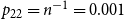 $p_{22}=n^{-1}=0.001$
and vary
$p_{22}=n^{-1}=0.001$
and vary
 $p_{12}=0.002$
,
$p_{12}=0.002$
,
 $0.004$
,
$0.004$
,
 $\ldots$
,
$\ldots$
,
 $0.02$
. As
$0.02$
. As
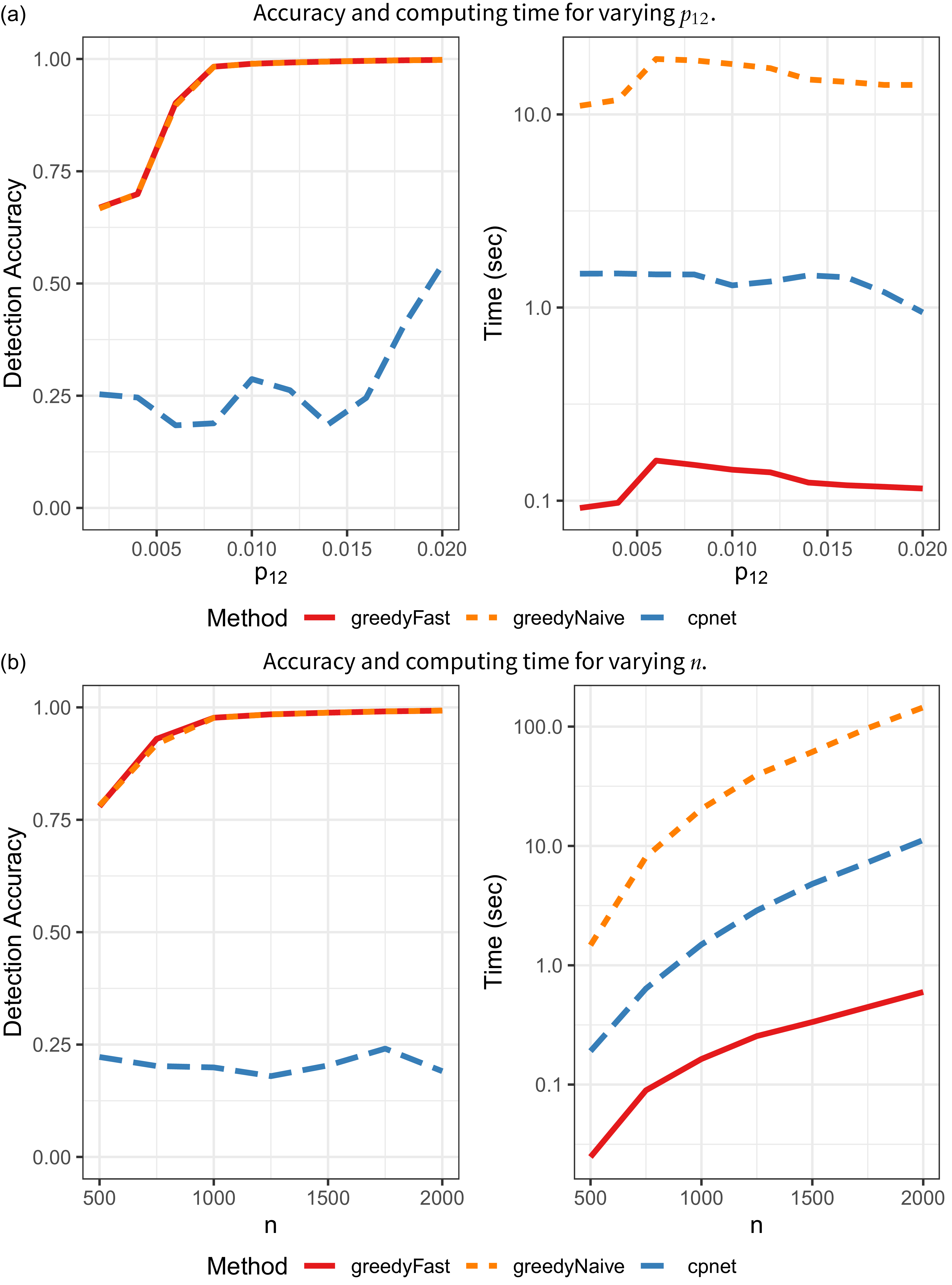
 $p_{12}$
increases, so too does the strength of the CP structure in the network. The results are in Figure 2a. greedyFast has a much larger detection accuracy and is approximately one order-of- magnitude faster than cpnet for all values of
$p_{12}$
increases, so too does the strength of the CP structure in the network. The results are in Figure 2a. greedyFast has a much larger detection accuracy and is approximately one order-of- magnitude faster than cpnet for all values of
 $p_{12}$
. As expected, greedyNaive yields identical accuracy results, but the proposed algorithmic improvement significantly decreases computing time. In the Appendix, we also rerun greedyFast on the same network multiple times to understand the effect of the stochasticity in the algorithm. In general, we find very small variance in terms of accuracy and run-time.
$p_{12}$
. As expected, greedyNaive yields identical accuracy results, but the proposed algorithmic improvement significantly decreases computing time. In the Appendix, we also rerun greedyFast on the same network multiple times to understand the effect of the stochasticity in the algorithm. In general, we find very small variance in terms of accuracy and run-time.
Next, we fix
 $p_{12}=0.005$
and
$p_{12}=0.005$
and
 $p_{22}=0.001$
and vary
$p_{22}=0.001$
and vary
 $n=500,750,\ldots ,2000$
with results in Figure 2b. Again, greedyFast clearly outperforms cpnet with superior accuracy, and is much faster than both the naive implementation and cpnet algorithm. It also appears that greedyFast and greedyNaive are more stable in both settings as the classification accuracy monotonically increases with
$n=500,750,\ldots ,2000$
with results in Figure 2b. Again, greedyFast clearly outperforms cpnet with superior accuracy, and is much faster than both the naive implementation and cpnet algorithm. It also appears that greedyFast and greedyNaive are more stable in both settings as the classification accuracy monotonically increases with
 $p_{12}$
and
$p_{12}$
and
 $n$
, unlike that of cpnet. Finally, in the Appendix, we present a log-log plot of the runtime with
$n$
, unlike that of cpnet. Finally, in the Appendix, we present a log-log plot of the runtime with
 $n$
to verify the algorithm’s computational complexity.
$n$
to verify the algorithm’s computational complexity.
4.2. Degree-corrected block model CP structure
In the second set of simulations, we generate networks from a degree-corrected block model (DCBM) (Karrer and Newman Reference Karrer and Newman2011). Namely, we introduce weight parameters
 $\boldsymbol \theta =(\theta _1,\ldots ,\theta _n)^\top$
to allow for degree heterogeneity among nodes, and generate networks with
$\boldsymbol \theta =(\theta _1,\ldots ,\theta _n)^\top$
to allow for degree heterogeneity among nodes, and generate networks with
 $P_{ij}=\theta _i\theta _jp_{c_i^*,c_j^*}$
. If
$P_{ij}=\theta _i\theta _jp_{c_i^*,c_j^*}$
. If
 $p_{11}\gt p_{12}\gt p_{22}$
, then we expect the resulting networks to exhibit a CP structure. We sample
$p_{11}\gt p_{12}\gt p_{22}$
, then we expect the resulting networks to exhibit a CP structure. We sample
 $\theta _i\stackrel {\text{iid.}}{\sim }\mathsf{Uniform}(0.6,0.8)$
and fix
$\theta _i\stackrel {\text{iid.}}{\sim }\mathsf{Uniform}(0.6,0.8)$
and fix
 $p_{22}=0.05$
. First, we fix
$p_{22}=0.05$
. First, we fix
 $n=1000$
and vary
$n=1000$
and vary
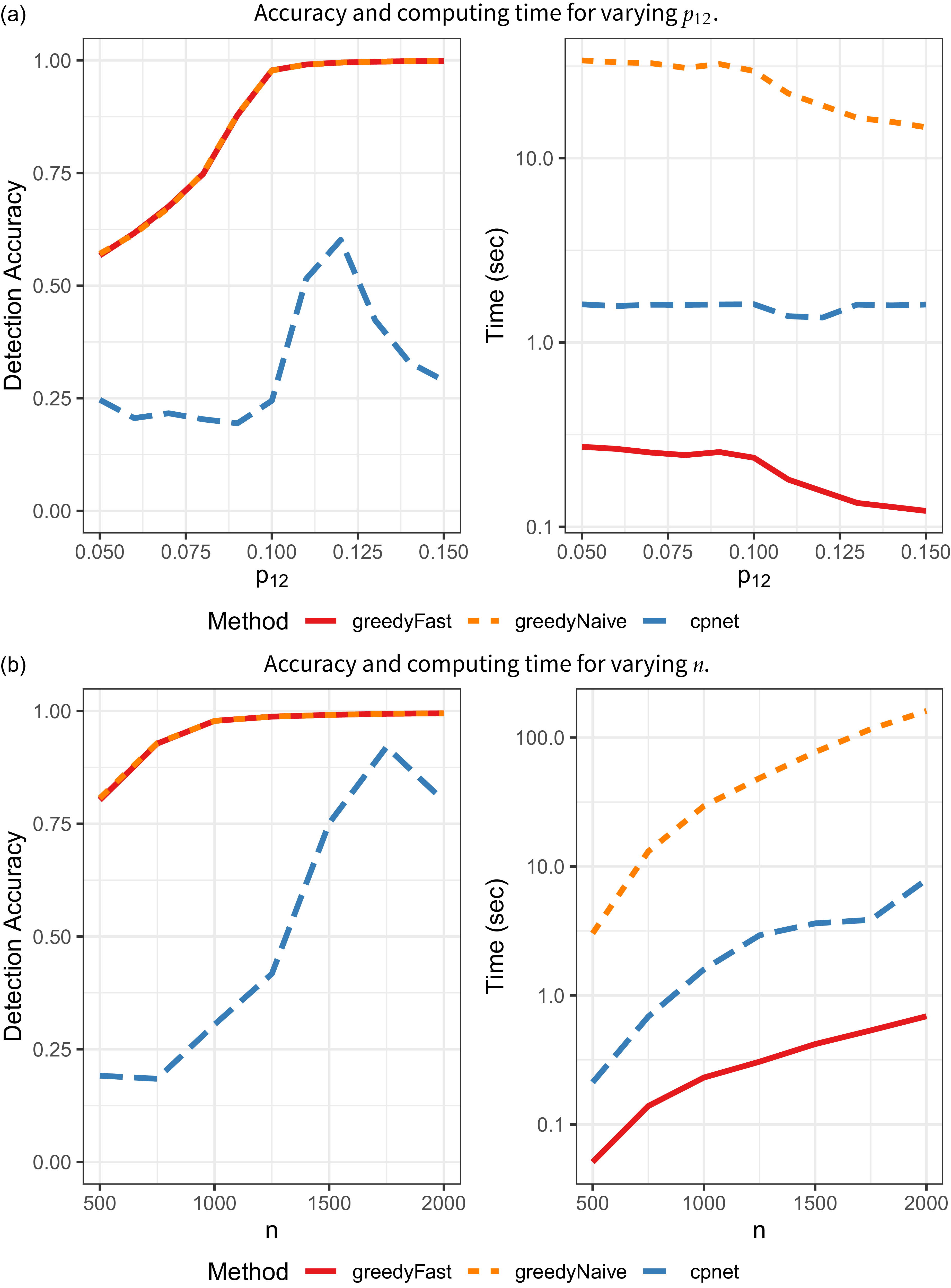
 $p_{12}=0.05, 0.06,\ldots , 0.15$
, with results in Figure 3a. Second, we fix
$p_{12}=0.05, 0.06,\ldots , 0.15$
, with results in Figure 3a. Second, we fix
 $p_{12}=0.10$
and vary
$p_{12}=0.10$
and vary
 $n=500,750,\ldots ,2000$
. As in the SBM examples, greedyFast yields the same accuracy as greedyNaive, but is markedly faster. It is also significantly faster and more accurate than the cpnet implementation.
$n=500,750,\ldots ,2000$
. As in the SBM examples, greedyFast yields the same accuracy as greedyNaive, but is markedly faster. It is also significantly faster and more accurate than the cpnet implementation.
CP identification results on DCBM networks.

5. Real-data analysis
Lastly, we apply greedyFast to thirteen real-world networks. We consider data sets of a variety of domains, sizes and densities to ensure the broad applicability of the method, including: UK Faculty (number of nodes
 $n=81$
, average edge probability
$n=81$
, average edge probability
 $\bar A=0.18$
) (Nepusz et al. Reference Nepusz, Petróczi, Négyessy and Bazsó2008), Email (
$\bar A=0.18$
) (Nepusz et al. Reference Nepusz, Petróczi, Négyessy and Bazsó2008), Email (
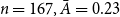 $n=167, \bar A=0.23$
) (Michalski et al. Reference Michalski, Palus and Kazienko2011), British MP (
$n=167, \bar A=0.23$
) (Michalski et al. Reference Michalski, Palus and Kazienko2011), British MP (
 $n=381, \bar A=0.08$
) (Greene and Cunningham Reference Greene and Cunningham2013), Congress (
$n=381, \bar A=0.08$
) (Greene and Cunningham Reference Greene and Cunningham2013), Congress (
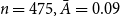 $n=475, \bar A=0.09$
) (Fink et al. Reference Fink, Fullin, Gutierrez, Omodt, Zinnecker, Sprint and McCulloch2023), Political Blogs (
$n=475, \bar A=0.09$
) (Fink et al. Reference Fink, Fullin, Gutierrez, Omodt, Zinnecker, Sprint and McCulloch2023), Political Blogs (
 $n=1224, \bar A=0.02$
) (Adamic and Glance Reference Adamic and Glance2005), DBLP (
$n=1224, \bar A=0.02$
) (Adamic and Glance Reference Adamic and Glance2005), DBLP (
 $n=2203, \bar A=0.47$
) (Gao et al. Reference Gao, Liang, Fan, Sun and Han2009; Ji et al. Reference Ji, Sun, Danilevsky, Han and Gao2010), Hospital (
$n=2203, \bar A=0.47$
) (Gao et al. Reference Gao, Liang, Fan, Sun and Han2009; Ji et al. Reference Ji, Sun, Danilevsky, Han and Gao2010), Hospital (
 $n=75, \bar A=0.41$
) (Vanhems et al. Reference Vanhems, Barrat, Cattuto, Pinton, Khanafer, Regis and Voirin2013), School (
$n=75, \bar A=0.41$
) (Vanhems et al. Reference Vanhems, Barrat, Cattuto, Pinton, Khanafer, Regis and Voirin2013), School (
 $n=242, \bar A=0.29$
) (Stehlé et al. Reference Stehlé, Voirin, Barrat, Cattuto, Isella, Pinton, Quaggiotto, Van den Broeck, Régis, Lina, Vanhems and Viboud2011), Bluetooth (
$n=242, \bar A=0.29$
) (Stehlé et al. Reference Stehlé, Voirin, Barrat, Cattuto, Isella, Pinton, Quaggiotto, Van den Broeck, Régis, Lina, Vanhems and Viboud2011), Bluetooth (
 $n=672, \bar A=0.10$
) (Sapiezynski et al. Reference Sapiezynski, Stopczynski, Lassen and Lehmann2019), Biological 1, 2, 3 (
$n=672, \bar A=0.10$
) (Sapiezynski et al. Reference Sapiezynski, Stopczynski, Lassen and Lehmann2019), Biological 1, 2, 3 (
 $n=2220,3289,4040, \bar A=0.02, 0.02, 0.01$
, respectively) (Cho et al. Reference Cho, Shin, Hwang, Kim, Shim, Kim and Lee2014), and Facebook (
$n=2220,3289,4040, \bar A=0.02, 0.02, 0.01$
, respectively) (Cho et al. Reference Cho, Shin, Hwang, Kim, Shim, Kim and Lee2014), and Facebook (
 $n=4039, \bar A=0.10$
) (Leskovec and Mcauley Reference Leskovec and Mcauley2012). All data was retrieved from (Csárdi et al. Reference Csárdi, Nepusz, Traag, Horvát, Zanini, Noom and Müller2025; Leskovec and Krevl Reference Leskovec and Krevl2014; Rossi and Ahmed Reference Rossi and Ahmed2015). For each network, we remove all edge weights, directions, time stamps, self-loops, etc. We also only consider two groups of researchers in the DBLP network as in Sengupta and Chen (Reference Sengupta and Chen2018). We run greedyFast and the cpnet algorithm to identify the optimal CP labels, and record
$n=4039, \bar A=0.10$
) (Leskovec and Mcauley Reference Leskovec and Mcauley2012). All data was retrieved from (Csárdi et al. Reference Csárdi, Nepusz, Traag, Horvát, Zanini, Noom and Müller2025; Leskovec and Krevl Reference Leskovec and Krevl2014; Rossi and Ahmed Reference Rossi and Ahmed2015). For each network, we remove all edge weights, directions, time stamps, self-loops, etc. We also only consider two groups of researchers in the DBLP network as in Sengupta and Chen (Reference Sengupta and Chen2018). We run greedyFast and the cpnet algorithm to identify the optimal CP labels, and record
 $T({\textbf {A}},\hat {\boldsymbol{c}})$
, the value of the BE metric evaluated at the optimal labels returned by each algorithm, the number of core nodes in these optimal labels and the computing time. Since ground-truth labels are unknown in these networks, achieving a higher objective value
$T({\textbf {A}},\hat {\boldsymbol{c}})$
, the value of the BE metric evaluated at the optimal labels returned by each algorithm, the number of core nodes in these optimal labels and the computing time. Since ground-truth labels are unknown in these networks, achieving a higher objective value
 $T({\textbf {A}},\hat {\boldsymbol{c}})$
is the main criterion to judge which algorithm returns superior labels. We run each Algorithm 10 times and keep the results corresponding to the largest value of the objective function (along with the total run-time). Results are reported in Table 1. In this section, we run the cpnet algorithm directly in Python to eliminate any time that might be added from using the reticulate package. In general, however, we found virtually no difference in the run-time or performance when using the function in R or Python.
$T({\textbf {A}},\hat {\boldsymbol{c}})$
is the main criterion to judge which algorithm returns superior labels. We run each Algorithm 10 times and keep the results corresponding to the largest value of the objective function (along with the total run-time). Results are reported in Table 1. In this section, we run the cpnet algorithm directly in Python to eliminate any time that might be added from using the reticulate package. In general, however, we found virtually no difference in the run-time or performance when using the function in R or Python.
Results of real-data analysis using greedyFast and cpnet.
 $T({\textbf {A}},\hat {\boldsymbol{c}})$
: value of objective function at optimal labels returned by the algorithm;
$T({\textbf {A}},\hat {\boldsymbol{c}})$
: value of objective function at optimal labels returned by the algorithm;
 $k$
: number of nodes assigned to the core in the optimal labels; time: computing time (seconds)
$k$
: number of nodes assigned to the core in the optimal labels; time: computing time (seconds)

Overall, the results demonstrate strong performance of the proposed method. In about half of the networks, the optimal value of the objective function is similar between the two algorithms, but greedyFast is consistently one to two orders of magnitude faster. On the remaining networks (British MP, Political Blogs, DBLP, Biological 1–3, Facebook), the proposed algorithm is not only faster than that of cpnet but also yields noticeably superior labels in terms of the value of
 $T({\textbf {A}},\hat {\boldsymbol{c}})$
. Moreover, on DBLP, greedyFast is
$T({\textbf {A}},\hat {\boldsymbol{c}})$
. Moreover, on DBLP, greedyFast is
 $217/0.630\approx 344$
times faster than the competing method. Additionally, our method appears to converge to a local optimum for all networks, but the cpnet algorithm seems not to in British MP, Biological 2 and Facebook. Even after rerunning the algorithm on these networks, the result did not improve. This could be a result of the cpnet algorithmic design where node labels are fixed after they have been swapped. In summary, the proposed algorithm yields better approximations for the global maximum at a fraction of the computation time.
$217/0.630\approx 344$
times faster than the competing method. Additionally, our method appears to converge to a local optimum for all networks, but the cpnet algorithm seems not to in British MP, Biological 2 and Facebook. Even after rerunning the algorithm on these networks, the result did not improve. This could be a result of the cpnet algorithmic design where node labels are fixed after they have been swapped. In summary, the proposed algorithm yields better approximations for the global maximum at a fraction of the computation time.
6. Conclusion
In this work, we detail a greedy, label-switching algorithm to quickly identify CP structure in networks. In comparisons with an existing algorithm, our greedy approach demonstrates superior CP label identification, while also being theoretically guaranteed to terminate at a local maximum. Additionally, by noting the mathematical relationship between the proposed and current CP labels, our implementation greatly reduces the computation time. Indeed, on both synthetic and real-world networks, we typically observe an order-of- magnitude improvement in algorithmic run-time.
There are several interesting avenues for future work. Precise theoretical results surrounding the conditions needed to obtain a global optimum would be worthwhile. Additionally, we focused on algorithmic speed-ups stemming from mathematical properties of the objective function. Considering more efficient network storage and data structures, however, could also improve the efficiency of the algorithm. For example, we currently compute
 $\sum _{k=1}^i A_{ik}\Delta _{ik}$
in
$\sum _{k=1}^i A_{ik}\Delta _{ik}$
in
 $\mathcal O(n)$
operations. But on sparse networks where
$\mathcal O(n)$
operations. But on sparse networks where
 $\mathsf{E}(A_{ij})=\rho _n P_{ij}$
for some sparsity parameter
$\mathsf{E}(A_{ij})=\rho _n P_{ij}$
for some sparsity parameter
 $\rho _n\to 0$
, if we use an edge list, then the sum could be computed in
$\rho _n\to 0$
, if we use an edge list, then the sum could be computed in
 $\mathcal O(n\rho _n)$
operations, leading to potentially large gains. Lastly, our algorithmic approach could be applied to generalizations of the BE metric, e.g., Estévez and Nordlund (Reference Estévez and Nordlund2025).
$\mathcal O(n\rho _n)$
operations, leading to potentially large gains. Lastly, our algorithmic approach could be applied to generalizations of the BE metric, e.g., Estévez and Nordlund (Reference Estévez and Nordlund2025).
Acknowledgments
We would like to thank Sadamori Kojaku for help understanding the cpnet algorithm. We also greatly appreciate the feedback and comments from the reviewers and editors.
Funding statement
None to report.
Competing interests
None to report.
Data availability statement
All data used in this study is freely available online.
Author contributions
Conceptualization: EY, SS. Methodology: EY. Coding: EY. Writing original draft: EY. Mentoring: SS. All authors approved the final submitted draft.
Ethical standards
N/A
Appendix
Proof of Proposition 1
Let
 $\hat {\boldsymbol{c}}_1$
be the labels returned by Algorithm 1. Then for all
$\hat {\boldsymbol{c}}_1$
be the labels returned by Algorithm 1. Then for all
 $\boldsymbol c\in N(\hat {\boldsymbol{c}}_1)$
,
$\boldsymbol c\in N(\hat {\boldsymbol{c}}_1)$
,
 $T({\textbf {A}},\hat {\boldsymbol{c}}_1)\geq T({\textbf {A}},\boldsymbol c)$
, i.e., Algorithm 1 converges to a local optimum.
$T({\textbf {A}},\hat {\boldsymbol{c}}_1)\geq T({\textbf {A}},\boldsymbol c)$
, i.e., Algorithm 1 converges to a local optimum.
Proof. Recall the steps of Algorithm 1. Then the result is immediate. Let
 $\hat {\boldsymbol{c}}_1$
be the labels that Algorithm 1 converged to. Assume, for contradiction, that there is some
$\hat {\boldsymbol{c}}_1$
be the labels that Algorithm 1 converged to. Assume, for contradiction, that there is some
 $\boldsymbol c'\in N(\hat {\boldsymbol{c}}_1)$
such that
$\boldsymbol c'\in N(\hat {\boldsymbol{c}}_1)$
such that
 $T({\textbf {A}},\boldsymbol c') \gt T({\textbf {A}},\hat {\boldsymbol{c}}_1)$
. But this is a contradiction because if
$T({\textbf {A}},\boldsymbol c') \gt T({\textbf {A}},\hat {\boldsymbol{c}}_1)$
. But this is a contradiction because if
 $T({\textbf {A}},\boldsymbol c') \gt T({\textbf {A}},\hat {\boldsymbol{c}}_1)$
, then Algorithm 1 would have swapped the differing labels such such that
$T({\textbf {A}},\boldsymbol c') \gt T({\textbf {A}},\hat {\boldsymbol{c}}_1)$
, then Algorithm 1 would have swapped the differing labels such such that
 $\hat {\boldsymbol{c}}_1=\boldsymbol c'$
. Therefore, it must be that
$\hat {\boldsymbol{c}}_1=\boldsymbol c'$
. Therefore, it must be that
 $T({\textbf {A}},\hat {\boldsymbol{c}}_1) \geq T({\textbf {A}},\boldsymbol c')$
for any
$T({\textbf {A}},\hat {\boldsymbol{c}}_1) \geq T({\textbf {A}},\boldsymbol c')$
for any
 $\boldsymbol c'\in N(\hat {\boldsymbol{c}}_1)$
.
$\boldsymbol c'\in N(\hat {\boldsymbol{c}}_1)$
.
Cpnet implementation
We now provide more details on the cpnet algorithm to find the optimal CP labels. This algorithm uses a Kernighan-Lin (Kernighan and Lin Reference Kernighan and Lin1970) approach. Specifically, the CP labels,
 $\boldsymbol c$
, are first randomly initialized to the core or periphery with equal probability. Then, for each node, the label of the node is switched and the change in the objective function (
$\boldsymbol c$
, are first randomly initialized to the core or periphery with equal probability. Then, for each node, the label of the node is switched and the change in the objective function (
 $T({\textbf {A}},\boldsymbol c)$
) is calculated. After swapping all
$T({\textbf {A}},\boldsymbol c)$
) is calculated. After swapping all
 $n$
nodes, the switch which led to the largest increase in the objective function value is kept. Then this node’s label is held fixed for the remainder of the algorithm and the process repeats. The algorithm terminates when the improvement in the objective function is less than or equal to
$n$
nodes, the switch which led to the largest increase in the objective function value is kept. Then this node’s label is held fixed for the remainder of the algorithm and the process repeats. The algorithm terminates when the improvement in the objective function is less than or equal to
 $\varepsilon =10^{-7}$
, or if all nodes have been checked.
$\varepsilon =10^{-7}$
, or if all nodes have been checked.
There are some key similarities and differences between this algorithm and greedyFast. First, both methods use a local-greedy search by swapping the label of a single node. On the other hand, greedyFast does not fix a node’s label once it has been swapped, and the node order is randomized each loop through the algorithm; in cpnet, this order is fixed throughout. Additionally, greedyFast swaps a node label immediately if it increases the objective function, not waiting until all nodes have been checked. It also has a different stopping condition, terminating the algorithm when all
 $n$
nodes have been swapped and none of them led to an increase in the objective function. Additionally, the default implementation in cpnet reruns the algorithm ten times with different initial labels, and then keeps only the result corresponding to the largest objective function value. This was changed to a single run for the simulation studies.
$n$
nodes have been swapped and none of them led to an increase in the objective function. Additionally, the default implementation in cpnet reruns the algorithm ten times with different initial labels, and then keeps only the result corresponding to the largest objective function value. This was changed to a single run for the simulation studies.
Sensitivity analysis
We briefly study the effect of the node order randomization in Algorithm 1. In the implementation of both greedyFast and greedyNaive, we randomly initialize the CP labels,
 $\boldsymbol c$
, as well as randomly shuffle the node order when swapping the CP membership assignments. To understand the effect of this stochasticity, we generate networks as in Section 4.1, i.e., SBM with
$\boldsymbol c$
, as well as randomly shuffle the node order when swapping the CP membership assignments. To understand the effect of this stochasticity, we generate networks as in Section 4.1, i.e., SBM with
 $n=1000$
,
$n=1000$
,
 $p_{11}=2p_{12}$
,
$p_{11}=2p_{12}$
,
 $p_{22}=0.001$
,
$p_{22}=0.001$
,
 $k=0.1n$
, and vary
$k=0.1n$
, and vary
 $p_{12}=0.002, 0.004,\ldots ,0.02$
. Instead of generating 100 networks for each parameter combination, we instead generate a single network but apply greedyFast to this same network 100 times. We report the accuracy and run-time in box-plots in Figure 4. Clearly, there is very little variance in the results, indicating minimal sensitivity to the randomization in Algorithm 1.
$p_{12}=0.002, 0.004,\ldots ,0.02$
. Instead of generating 100 networks for each parameter combination, we instead generate a single network but apply greedyFast to this same network 100 times. We report the accuracy and run-time in box-plots in Figure 4. Clearly, there is very little variance in the results, indicating minimal sensitivity to the randomization in Algorithm 1.
Accuracy and computing boxplots for sensitivity analysis.

Log runtime against log
 $n$
for the SBM simulations.
$n$
for the SBM simulations.

Runtime complexity
We further compare the runtime of the various algorithms. In Figure 5, we plot the log runtime against the log number of nodes for the SBM synthetic network simulations. We also regress log runtime on log
 $n$
for each algorithm and find that the slope is 3.2, 2.9 and 2.2 for greedyNaive, cpnet and greedyFast, respectively. For the DCBM simulations, the respective fitted slopes are 2.8, 2.5 and 1.8. These results further validate the computational improvements of the proposed implementation.
$n$
for each algorithm and find that the slope is 3.2, 2.9 and 2.2 for greedyNaive, cpnet and greedyFast, respectively. For the DCBM simulations, the respective fitted slopes are 2.8, 2.5 and 1.8. These results further validate the computational improvements of the proposed implementation.


 Open access