


Nomenclature
- $A\;$
$A\;$
-
planform area of the main wing (m2)
-
$AR\;$
-
aspect ratio
-
$C_{D}$
-
drag coefficient
-
$C_{D_{induced}}$
-
induced drag coefficient
-
$C_{D_{parasite}}$
-
parasite drag coefficient
-
${C_L}\;\;$
-
lift coefficient
-
${E_{op}}\;$
-
operational effectiveness metric
-
${E_l}\;$
-
layer effectiveness vector
-
${H_f}$
-
firepower health
-
${P_{detection}}\;$
-
detection probability of an asset
-
${R_{MS}}\;$
-
mission success rate (MSR)
-
${R_{MD}}\;$
-
mission damage rate (MDR)
-
$Re$
-
Reynolds number
-
$RCS\;$
-
radar cross section (dBsm, m2)
-
${W_{MTOW\;}}\;$
-
maximum takeoff weight of the UAV (kg)
-
$W_{emp}$
-
empty weight of the UAV (kg)
-
${W_{fuel}}\;$
-
fuel weight of the UAV (kg)
-
${W_{payload}}\;$
-
payload weight of the UAV (kg)
-
$SFC$
-
Specific fuel consumption


Greek symbols
-
$\alpha \;\;$
-
angle-of-attack (degrees)
-
$\theta \;\;$
-
elevation angle
-
$\lambda \;\;$
-
taper ratio
-
${\rm{\Lambda \;\;}}$
-
sweep angle (degrees)
-
$\phi \;\;$
-
azimuth angle


1.0 Introduction
The future battlefield is rapidly evolving into a domain where unmanned combat systems, enhanced by significant advances in autonomy and artificial intelligence (AI), will play a central role. These systems, particularly unmanned combat aerial vehicles (UCAVs), are now essential to modern military scenarios. UCAVs are expected to be crucial across a wide range of operations, including intelligence, surveillance and reconnaissance (ISR), electronic warfare, air combat and ground attack missions. The operational capabilities of UCAVs often vary significantly, depending on the mission type and specific requirements. Furthermore, operational costs, which generally increase with vehicle capabilities, are a critical factor, making optimal fleet composition and asset characteristics complex to determine. To address this, a model-based approach can be employed to simulate operations in a digital environment, enabling the identification of the optimal fleet components and requirements necessary for mission success.
UCAVs designed for mission-oriented operations must strike a balance between performance, modularity and cost-efficiency. Modularity enables UAVs to adapt to diverse mission requirements through configurable payloads, sensors and aerodynamic structures. This flexibility is particularly advantageous in contested environments where rapid adaptability is essential. These UAVs include both attritable and reusable configurations, allowing deployment flexibility for a wide range of missions [Reference Gunzinger and Autenried1]. Attritable UAVs, characterised by their low cost and expendability, represent a new category of low-cost drones that can be deployed in high-risk scenarios where losses are acceptable. Conversely, reusable configurations are designed for long-term use in sustained operations, providing reliability in prolonged engagements. In the U.S. Air Force’s Collaborative Combat Aircraft (CCA) programme, attritable platforms are emphasised for their potential to complement manned systems in roles such as electronic warfare, ISR and air-to-air combat, leveraging AI to enhance operational collaboration [2]. Similarly, the RAF’s Autonomous Collaborative Platform (ACP) strategy focuses on developing modular, low-cost systems that integrate advanced autonomy and human-machine teaming to address high-risk operational environments [3]. As shown in Fig. 1, modular UCAV designs facilitate rapid reconfiguration to address varying operational needs, enhancing mission adaptability.
Modular UAV design enabling mission-specific adaptability (adapted from Ref. (Reference Gunzinger and Autenried1)).

In this context, mission-based design emerges as a critical methodology for aligning system capabilities with operational demands. This approach provides a systematic framework for addressing the diverse requirements of UCAV operations by tailoring system design specifically to the requirements of the missions they will perform. Detailed operational scenarios that encompass mission objectives, environmental conditions and potential threats are central to this methodology and serve as a blueprint to guide the engineering and design process. Such scenarios facilitate the evaluation of trade-offs among design parameters, including survivability, lethality, and costs, ensuring that each design choice contributes to the system’s overall effectiveness within its intended mission environment.
The literature highlights several advancements in mission-based design. Albuquerque et al. [Reference Albuquerque, Gamboa and Silvestre4] developed a multidisciplinary optimisation methodology for adaptive aircraft design, incorporating low-fidelity models to efficiently evaluate early-stage designs. Their approach tailored design parameters such as wing area and engine thrust to specific mission phases, achieving significant improvements in mission effectiveness. Clark et al. [Reference Clark, Allison, Bae and Forster5] proposed an effectiveness-based design framework that integrates multidisciplinary design optimisation, uncertainty quantification and nondeterministic surrogate modeling to refine aircraft configurations under complex and uncertain mission conditions. This method emphasised mission-specific metrics, such as the probability of mission success, and employed advanced simulation techniques to assess trade-offs among various design options. Pagan et al. [Reference Pagan, Huynh, Schafer, Pinon-Fischer and Mavris6] presented a methodology combining Monte Carlo simulations and surrogate modeling to optimise UAV designs for Air Interdiction and ISR missions. Their work demonstrated the effectiveness of balancing cost-efficiency and operational performance through iterative evaluations of vehicle architectures and mission parameters. Similarly, Aleisa et al. [Reference Aleisa, Kontis, Pirlepeli and Nikbay7] proposed a mission-oriented optimisation approach for a non-constant swept flying-wing UCAV, utilising multi-fidelity surrogate modeling to enhance aerodynamic performance tailored to specific mission profiles. Klaproth et al. [Reference Klaproth, Bäuerle and Hornung8] introduced a multi-fidelity aerodynamic modeling approach within a mission-based UAV design process, leveraging hierarchical Kriging to optimise computational efficiency while maintaining high accuracy across the design space. Sells and Crossley [Reference Sells and Crossley9] developed a decision-making framework for small unmanned aircraft systems (UAS) fleet design, integrating mission customer preferences into a multi-objective optimisation process to align fleet configurations with operational demands effectively. Setayandeh and Babaei [Reference Setayandeh and Babaei10] proposed a system-of-systems optimisation strategy for UAV networks, enabling coordinated task allocation and resource sharing to maximise mission effectiveness in complex operational environments. Additionally, Chaudemar et al. [Reference Chaudemar, Aıello, de Saqui-Sannes and Poitou11] explored a mission-based UAV design methodology leveraging the Goal-Requirements Language (GRL) framework. Their work emphasised the importance of aligning UAV capabilities with mission-specific goals through rigorous modeling and validation, demonstrating how such an approach enhances the system’s adaptability and effectiveness in dynamic environments. In addition, recent MDO studies align with a mission-centric perspective. Zhang et al. [Reference Zhang, Yan, Huang, Che and Wang12] presented a bi-level, system-integrated optimisation that treats the climb mission as a system-level driver and reported about a 10% reduction in minimum climb time by co-optimising configuration variables with trajectory. Shen et al. [Reference Shen, Huang, Yan and Zhang13] demonstrated constraint-preserving three-dimensional shape parameterisation combined with surrogate-assisted multi-objective optimisation to balance lift-to-drag, internal volume use and thermal loads. To address computational cost at mission scale, Leng et al. [Reference Leng14] proposed a multi-fidelity, data-mining-guided framework that explores the design space with inexpensive estimates and then refines promising solutions with viscous computational fluid dynamics (CFD), reporting range improvements; the same approach was extended to combined boost–glide scenarios while maintaining consistency with system-level constraints [Reference Leng, Xie, Huang, Shen and Wang15]. A recent survey by Leng et al. [Reference Leng, Wang, Huang, Shen and An16] consolidates efficiency-oriented practices for aircraft MDO, including dimensionality-reduction of design variables, advanced three-dimensional shape parameterisation, MDO strategy selection and the use of machine learning to extract knowledge from optimisation data. Collectively, these methodologies illustrate the transformative potential of mission-based design. By integrating advanced modeling techniques, probabilistic frameworks and multi-objective decision-making strategies, these approaches enable the development of UAV systems that are not only cost-effective but also highly responsive to the complexities of modern operational environments.
Mission-based design optimisation requires a simulation environment that accurately reflects the complexity and variability of real-world scenarios. Uncertainty in the simulation environment directly influences the reliability of optimisation outcomes, as it allows for testing system performance under diverse and dynamic conditions. This consideration is particularly critical in mission planning systems, where adaptability and resilience are essential for success. Modern mission planning systems play a critical role in this context by facilitating efficient and dynamic coordination of assets in defense operations. These systems provide essential capabilities for mission simulation, including task assignment, path planning, and resource allocation. In this context, advanced mission planning tools such as BAE Systems’ SCEPTRE [17], Anduril’s Lattice [18], General Dynamics’ IMPACT [19], Lockheed Martin’s MDSET [20] and Saab’s MSS [Reference Saab21] illustrate the range of capabilities available to support adaptive and coordinated defense operations.
While these advanced mission planning tools significantly enhance operational capabilities, wargaming techniques offer an alternative approach for simulating operations and testing different strategies. Wargaming, broadly defined as the simulation of military operations using structured rules, data and methods, has a rich history dating back to the early 19th century [22]. This approach allows for detailed modeling of battlefield dynamics, including terrain effects, force distributions and adversarial strategies, which are often challenging to capture in traditional mission planning systems [Reference Hershkovitz23]. In the context of mission simulation, wargaming enables probabilistic evaluations of multiple scenarios, incorporating uncertainties and adversarial behaviours into the analysis. For instance, Filho et al. applied wargaming to optimise UAV positioning in beyond visual range combat scenarios, effectively accounting for enemy movement and dynamic interactions [Reference De Lima Filho24]. Similarly, Chen et al. demonstrated the application of wargaming simulations to urban flood disaster scenarios, highlighting their utility in optimising emergency management strategies through dynamic modeling and decision-tree analysis, demonstrating the adaptability of such techniques beyond military applications [Reference Chen, Zhang and Sun25]. These examples highlight the versatility of wargaming in modeling complex systems and testing various strategies.
In this work, we introduce a novel mission-centric design optimisation framework that directly addresses the complexities of designing UCAVs for diverse and contested operational environments. Unlike existing approaches, which often rely on isolated disciplinary models or simplified scenarios, our framework explicitly integrates complex mission dynamics into the design process. By combining wargaming-based simulations with multidisciplinary design optimisation (MDO), we establish a unified environment where aerodynamic, radar cross section and structural models are jointly evaluated under realistic mission conditions. Furthermore, we employ artificial neural network (ANN)-based surrogate models to accelerate analysis and enable rapid exploration of the design space. This contribution advances the state of the art by linking mission-level uncertainties with system-level design choices in a single, computationally efficient framework, thereby enabling the development of robust and adaptive UCAV configurations tailored to mission-centric requirements.
This paper is organised as follows: Section 2 introduces the mission-centric design optimisation framework together with the integration of wargaming-based simulations and surrogate driven multidisciplinary design optimisation. Section 3 details the methodology, including the multidisciplinary design optimisation process and the mission simulation algorithm. Section 4 presents the model simulation and results, including the simulation environment, evaluation metrics and comprehensive use cases in aerial combat and ground attack scenarios. Finally, Section 5 summarises the findings and discusses their implications for advancing mission-based UAV design optimisation.
2.0 Mission-centric design optimisation for UAVs
Mission-centric design optimisation systematically tailors UAV designs to meet specific mission objectives and operational needs. Unlike traditional methodologies that often aim for generic performance goals, this approach ensures UAVs are optimised for cost-efficiency, adaptability and mission-specific performance.
Representation of operational environment with multi-domain assets.

To address this challenge, an intelligent wargaming approach [Reference Yuksek, Guner, Karali, Candan and Inalhan26] has been further refined and a combat model enhanced to serve as the basis for the mission simulation environment. This environment is integrated with a surrogate-driven MDO algorithm specifically developed for UAVs [Reference Karali, Inalhan and Tsourdos27]. As illustrated in Fig. 2, the framework models a multi-domain, multi-asset operational environment. This includes interactions across aerial, ground and naval layers to provide a realistic simulation. The framework leverages mathematical models to automatically explore possible scenarios, assess outcomes and identify optimal design configurations. By automating this process, the framework enables systematic exploration of design options to address the complex requirements of diverse operational environments.
Overview of the mission-centric design optimisation approach for UAVs.

To enhance adaptability, the framework incorporates modular UAV designs, enabling rapid reconfiguration through interchangeable payloads, sensors and aerodynamic structures. Figure 3 illustrates the framework’s workflow, from fleet configuration to mission simulation and optimisation. The simulation environment integrates automated target assignment, optimal path generation and a probabilistic combat model to reflect real-world mission complexities. Through iterative simulations under diverse conditions, the framework evaluates trade-offs among survivability, lethality and cost to determine optimal configurations.
3.0 Methodology
The methodology consists of two main components. The first one is the Multidisciplinary Design Optimisation component, which incorporates a multidisciplinary design and optimisation loop and utilises deep neural networks based surrogate models from various sub-disciplines. Through multi-objective optimisation, a Pareto set is obtained, balancing different objective functions. Within the simulation loop, the configuration that maximises operational effectiveness is selected from the Pareto set, allowing for the formation of the most suitable fleet component for the mission.
The second component is the Mission Simulation Environment, which includes three subcomponents: task assignment, path planning and the combat model. Since the simulation is dependent on probabilistic variables, it is run hundreds of times to explore different probabilistic outcomes. The results of these simulations are evaluated using various evaluation metrics to assess operational effectiveness. Based on these evaluations, the process iteratively refines the designs and informs the optimisation framework. The general framework for the mission-centric design optimisation process is illustrated in Fig. 4.
General framework for mission-centric design optimisation process.

The following subsections provide a detailed explanation of the multidisciplinary design optimisation, including the integration of deep neural networks driven surrogate models and multi-objective optimisation techniques, and the Mission Simulation Framework, which includes task assignment, path planning and the battle model. Together, these components are combined to achieve optimal mission outcomes.
3.1 Multidisciplinary design optimisation
Design optimisation of UCAVs is a complex, multidisciplinary challenge that involves trade-offs between performance criteria such as aerodynamic efficiency, structural integrity, stealth and mission-specific capabilities. In this section, we describe a framework that integrates MDO with advanced surrogate models to achieve optimal UCAV configurations to meet specific operational requirements [Reference Karali, Inalhan and Tsourdos27].
The process begins with the initial sizing of the UCAV based on fundamental flight performance criteria such as wing loading and thrust-to-weight ratio. These parameters are derived from mission requirements, including maximum speed, range and climbing rate. The initial sizing algorithm generates a feasible design space, which is then explored using a genetic algorithm-based search method to identify the optimal configuration. To accelerate the optimisation process and reduce computational costs, deep learning-based surrogate models are employed. These models are trained on several thousand low- and mid-fidelity simulations covering the design space. Once trained, the surrogate models provide predictions of key performance metrics, such as lift and total drag coefficients, structural weight and radar cross section, in near real-time. Compared to high-fidelity CFD and finite element analysis (FEA), which require significantly longer runtimes for each evaluation, the surrogate models enable rapid exploration of the design space. Their accuracy has been validated, with coefficients of determination ( ${R^2}$
) around 0.99 and mean absolute percentage errors (MAPE) typically within 2–3%. This balance of speed and fidelity makes them suitable for screening and ranking candidate configurations during the optimisation process.
${R^2}$
) around 0.99 and mean absolute percentage errors (MAPE) typically within 2–3%. This balance of speed and fidelity makes them suitable for screening and ranking candidate configurations during the optimisation process.
As outlined in the subsequent sections, the MDO framework is systematically developed through detailed modeling and analysis. Initially, the fundamental components of the UAV model are described, including Aerodynamics, Radar Cross Section (RCS), Structures and Propulsion & Weight modules. These models form the basis for evaluating key performance metrics and constraints. Following this, the development and integration of ANN-based surrogate models are detailed, highlighting their role in accelerating performance predictions. Finally, the optimisation methodology is presented to illustrate the iterative process of achieving optimal UAV configurations across multiple competing objectives.
3.1.1 Aerodynamics
Aerodynamic performance plays a vital role in analysing the forces that UAVs experience during flight and how these forces influence their behaviour. In UAV design, aerodynamic efficiency strongly affects overall flight performance and also provides essential inputs for structural analysis and propulsion system evaluation.
Among the available methods, the panel method is particularly advantageous for UAV configurations because of its low computational cost and fast turnaround. It solves the potential-flow equations at subsonic or supersonic free-stream Mach numbers [Reference Katz and Plotkin28]. The governing equation is the Prandtl–Glauert formulation,
 \begin{equation}{\tilde \nabla ^2}\phi = \!\left({1 - M_\infty ^2} \right){\phi _{xx}} + {\phi _{yy}} + {\phi _{zz}} = 0\end{equation}
where $\phi $
is the velocity potential and
$\phi $
is the velocity potential and ${M_\infty }$
is the free-stream Mach number. To model the effect of geometry on the flow, singularities are distributed over the surfaces to satisfy boundary conditions.
${M_\infty }$
is the free-stream Mach number. To model the effect of geometry on the flow, singularities are distributed over the surfaces to satisfy boundary conditions.
From the resulting velocity field, pressure coefficients are computed as
 \begin{equation}{C_p} = 1 - {\!\left({\frac{V}{{{V_\infty }}}} \right)^2}\end{equation}
and integrated to obtain aerodynamic forces and moments:
 \begin{equation}{\bf{F}} = \mathop \int \nolimits_S p{\bf{n}}{\rm{\;}}dS\end{equation}
where $p$
is surface pressure,
$p$
is surface pressure, ${\bf{n}}$
is the normal vector and
${\bf{n}}$
is the normal vector and $S$
is the surface area.
$S$
is the surface area.
Because the panel method accounts mainly for induced drag, additional semi-empirical correlations are used to estimate parasite contributions such as form, skin-friction and interference drag. The total drag is then expressed as
 \begin{equation}{C_{{D_{{\rm{total}}}}}} = {C_{{D_{{\rm{induced}}}}}} + {C_{{D_{{\rm{parasite}}}}}}\end{equation}
In this framework, the panel code is not part of the optimisation loop but is used offline as a training-data generation tool. By sampling the design space and labeling each configuration with aerodynamic responses, it enables the construction of surrogate models that provide rapid predictions during optimisation. Limited validation against higher-fidelity references is performed to maintain conservative margins where required. This balance between accuracy and efficiency is appropriate for early-stage UAV design studies, where thousands of evaluations are needed and aerodynamic metrics serve directly as inputs to structures, propulsion and mission-level analyses.
3.1.2 Radar cross section
The RCS quantifies how detectable an object is by radar, representing the effective area that reflects radar signals back to the receiver. RCS is influenced by factors such as the object’s geometry, material composition, radar signal frequency, polarisation and the relative positions of antennas [Reference Karakoc and Kaya29]. Mathematically, RCS is defined as:
 \begin{equation}\sigma = 4\pi \mathop {{\rm{lim}}}\limits_{R \to \infty } \!\left({{R^2}\frac{{{{\left| {{{\bf{E}}^{r}}} \right|}^2}}}{{{{\left| {{{\bf{E}}^t}} \right|}^2}}}} \right)\end{equation}
where $R$
is the range, and
$R$
is the range, and ${{\bf{E}}^r}$
and
${{\bf{E}}^r}$
and ${{\bf{E}}^t}$
represent the magnitudes of the backscattered and incident electric fields, respectively. RCS is typically expressed in square meters (
${{\bf{E}}^t}$
represent the magnitudes of the backscattered and incident electric fields, respectively. RCS is typically expressed in square meters ( ${{\rm{m}}^2}$
) or in decibels relative to a square meter (dBsm), with the conversion given by:
${{\rm{m}}^2}$
) or in decibels relative to a square meter (dBsm), with the conversion given by:
 \begin{equation}\sigma \left[ {{\rm{dBsm}}} \right] = 10 {\rm{log}}\!\left(\sigma \right)[{{{\rm{m}}^2}}]\end{equation}
RCS is inherently variable, depending on factors such as viewing angles, frequency and material properties. To simplify the analysis, a mean RCS value ( $\bar \sigma $
) is often used, calculated as:
$\bar \sigma $
) is often used, calculated as:
 \begin{equation}\bar \sigma = {1 \over {\!\left({{\theta _2} - {\theta _1}} \right)\!\left({{\phi _2} - {\phi _1}} \right)}}\mathop \int\nolimits_{{\theta _1}}^{{\theta _2}} \mathop \int \nolimits_{{\phi _1}}^{{\phi _2}} \sigma\!\left({\theta ,\phi } \right){\rm{\;}}d\phi {\rm{\;}}d\theta \end{equation}
where $\bar \sigma $
represents the mean RCS,
$\bar \sigma $
represents the mean RCS, $\sigma \!\left({\theta ,\phi } \right)$
is the RCS as a function of the elevation angle
$\sigma \!\left({\theta ,\phi } \right)$
is the RCS as a function of the elevation angle $\theta $
and the azimuth angle
$\theta $
and the azimuth angle $\phi $
. The limits
$\phi $
. The limits ${\theta _1}$
and
${\theta _1}$
and ${\theta _2}$
define the range of the elevation angle, while
${\theta _2}$
define the range of the elevation angle, while ${\phi _1}$
and
${\phi _1}$
and ${\phi _2}$
define the range of the azimuth angle. This equation calculates the average RCS over a specified angular region in the
${\phi _2}$
define the range of the azimuth angle. This equation calculates the average RCS over a specified angular region in the $\theta $
and
$\theta $
and $\phi $
domains.
$\phi $
domains.
Numerical methods for RCS simulation fall into two categories: full-wave and asymptotic. Full-wave methods like the finite element method are accurate but computationally expensive, especially for high-frequency applications. Asymptotic methods, such as physical optics (PO) and ray tracing, are computationally efficient. PO is effective for convex surfaces, while ray tracing handles multi-scattering problems in concave geometries [Reference Peng, Li and Uysal30]. This study combines PO and ray tracing for RCS simulation of the aerial vehicle’s 3D surface model [Reference Peng31].
The RCS calculations are performed on the triangular surface meshes, and the simulations assume fixed signal properties across all cases, including a transmitted signal frequency of $f = 9{\rm{\;GHz}}$
. This frequency was chosen because it falls within the X-band range (8–12 GHz), which is the most commonly used frequency band for military aerial vehicle RCS analyses. The X-band is preferred due to its shorter wavelengths, which allow for effective resolution of the geometric and structural details of aircraft. Additionally, most air-to-air radar systems in military applications operate in this band, making it highly relevant for such analyses. The observation angles are set with
$f = 9{\rm{\;GHz}}$
. This frequency was chosen because it falls within the X-band range (8–12 GHz), which is the most commonly used frequency band for military aerial vehicle RCS analyses. The X-band is preferred due to its shorter wavelengths, which allow for effective resolution of the geometric and structural details of aircraft. Additionally, most air-to-air radar systems in military applications operate in this band, making it highly relevant for such analyses. The observation angles are set with $\phi $
ranging from
$\phi $
ranging from ${0^ \circ }$
to
${0^ \circ }$
to ${360^ \circ }$
, enabling the measurement of the RCS from all possible azimuthal directions. The elevation angle (
${360^ \circ }$
, enabling the measurement of the RCS from all possible azimuthal directions. The elevation angle ( $\theta $
) is fixed at
$\theta $
) is fixed at ${90^ \circ }$
, as this configuration corresponds to the radar and the aircraft being in the same horizontal plane. This setup is particularly useful for analysing the RCS of aircraft from a profile view, which is a frequent focus in RCS studies. This standardised setup ensures consistency and comparability across cases, enabling detailed evaluation of the RCS under controlled conditions.
${90^ \circ }$
, as this configuration corresponds to the radar and the aircraft being in the same horizontal plane. This setup is particularly useful for analysing the RCS of aircraft from a profile view, which is a frequent focus in RCS studies. This standardised setup ensures consistency and comparability across cases, enabling detailed evaluation of the RCS under controlled conditions.
3.1.3 Structures
Structural models are fundamental in the aircraft design process, particularly in the early stages when rapid and flexible evaluation of alternatives is essential. Simplified methodologies enable quick estimation of structural weight, guiding the development of more efficient designs without resorting to high-fidelity simulations.
In this study, two structural models are employed. A simplified shell model is applied to the fuselage, allowing for geometry-based weight estimation [Reference Roskam32, Reference Raymer33]. For the lifting surfaces, which bear the main structural loads, an efficient beam-element finite element model is used [Reference Jasa, Hwang and Martins34]. The structural response is governed by the standard equilibrium relation
 \begin{equation} K\vec u =\ \vec{\!f},\end{equation}
where $K$
is the global stiffness matrix,
$K$
is the global stiffness matrix, $\vec u$
the displacement vector and
$\vec u$
the displacement vector and $\vec{\!f}$
the applied loads. The formulation is designed to capture the dominant structural behaviours, such as axial stretching, bending about the principal axes and torsional resistance, through effective stiffness parameters (
$\vec{\!f}$
the applied loads. The formulation is designed to capture the dominant structural behaviours, such as axial stretching, bending about the principal axes and torsional resistance, through effective stiffness parameters ( $E$
,
$E$
, $G$
,
$G$
, ${I_y}$
,
${I_y}$
, ${I_z}$
,
${I_z}$
, $J$
,
$J$
, $A$
,
$A$
, $L$
). These parameters collectively represent the contribution of material and geometric properties to stiffness, making it possible to characterise structural response without reproducing the full element stiffness matrices, which are well established in the literature.
$L$
). These parameters collectively represent the contribution of material and geometric properties to stiffness, making it possible to characterise structural response without reproducing the full element stiffness matrices, which are well established in the literature.
Aerodynamic loads are mapped onto the structure as nodal forces along the span, enabling deflection and stress proxies to be checked against limits such as material yield and buckling. The model thus provides both a structural weight estimate and feasibility checks. These outputs are used offline to generate training data for surrogate models; during optimisation, the surrogate replaces the FEA, ensuring computational efficiency.
This hybrid approach, combining beam-based FEM for lifting surfaces and simplified shell analysis for the fuselage, yields more reliable estimates than purely statistical methods while maintaining computational efficiency for multidisciplinary design studies.
3.1.4 Propulsion and weight
In the design of the proposed high-subsonic UAV, the propulsion system and weight calculation are tightly integrated to optimise performance. The propulsion system is modeled for jet engines, with fuel weight calculated based on specific fuel consumption (SFC). The SFC quantifies the engine’s efficiency, relating fuel burn to the generated thrust:
 \begin{equation} {\rm{SFC}} = \frac{{{{\dot m}_{fuel}}}}{T}\end{equation}
where ${\dot m_{fuel}}$
is the mass flow rate of fuel, and
${\dot m_{fuel}}$
is the mass flow rate of fuel, and $T$
is the thrust generated by the engine. The total fuel weight is derived from mission requirements and aerodynamic performance, with the fuel requirement primarily governed by the mission profile. For a standard mission without payload release, fuel weight is the difference between take-off and landing weights:
$T$
is the thrust generated by the engine. The total fuel weight is derived from mission requirements and aerodynamic performance, with the fuel requirement primarily governed by the mission profile. For a standard mission without payload release, fuel weight is the difference between take-off and landing weights:
 \begin{equation} {W_{{\rm{fuel}}}} = {W_{{\rm{take}} - {\rm{off}}}} - {W_{{\rm{landing}}}}\end{equation}
where ${W_{{\rm{fuel}}}}$
represents the total fuel weight,
${W_{{\rm{fuel}}}}$
represents the total fuel weight, ${W_{{\rm{take}} - {\rm{off}}}}$
is the take-off weight, and
${W_{{\rm{take}} - {\rm{off}}}}$
is the take-off weight, and ${W_{{\rm{landing}}}}$
is the landing weight. Alongside propulsion, the weight module plays a critical role in determining UAV capabilities. The maximum take-off weight (MTOW) comprises the empty weight, payload weight and fuel weight:
${W_{{\rm{landing}}}}$
is the landing weight. Alongside propulsion, the weight module plays a critical role in determining UAV capabilities. The maximum take-off weight (MTOW) comprises the empty weight, payload weight and fuel weight:
 \begin{equation} {W_{{\rm{MTOW}}}} = {W_{{\rm{empty}}}} + {W_{{\rm{payload}}}} + {W_{{\rm{fuel}}}}\end{equation}
where ${W_{{\rm{MTOW}}}}$
is the maximum take-off weight,
${W_{{\rm{MTOW}}}}$
is the maximum take-off weight, ${W_{{\rm{empty}}}}$
is the empty weight of the vehicle (including structure, engine, and systems),
${W_{{\rm{empty}}}}$
is the empty weight of the vehicle (including structure, engine, and systems), ${W_{{\rm{payload}}}}$
is the weight of the payload and
${W_{{\rm{payload}}}}$
is the weight of the payload and ${W_{{\rm{fuel}}}}$
is the calculated fuel weight.
${W_{{\rm{fuel}}}}$
is the calculated fuel weight.
The weights calculated in the structural module, together with the engine system from the propulsion module, contribute to determining the empty weight of the aircraft. The structural module accounts for the weight of components such as the wings, tail, fuselage and landing gear, while the propulsion module adds the engine weight. In cases where the maximum take-off weight ( ${W_{{\rm{MTOW}}}}$
) is predefined, the algorithm utilises Equation (11) to compute the payload capacity based on the calculated empty weight and fuel weight. In this manner, variations in the structural module’s design directly influence the empty weight, which in turn affects the payload capacity. This iterative approach ensures that structural changes are dynamically reflected in the optimisation process, enabling efficient evaluation of the trade-offs between aerodynamic, structural and propulsion parameters.
${W_{{\rm{MTOW}}}}$
) is predefined, the algorithm utilises Equation (11) to compute the payload capacity based on the calculated empty weight and fuel weight. In this manner, variations in the structural module’s design directly influence the empty weight, which in turn affects the payload capacity. This iterative approach ensures that structural changes are dynamically reflected in the optimisation process, enabling efficient evaluation of the trade-offs between aerodynamic, structural and propulsion parameters.
3.1.5 Artificial neural network modeling
ANNs are employed in this study as surrogate models to replace computationally expensive simulations, enabling efficient and accurate predictions of UAV performance metrics. These metrics include aerodynamic coefficients, RCS and structural weight, which are critical for UAV design optimisation. By leveraging ANNs, the iterative optimisation process is significantly accelerated without compromising on the accuracy of predictions.
Input and output parameters for neural network modeling

The modeling process begins with the generation of a comprehensive dataset using Latin Hypercube Sampling (LHS). This statistical method ensures uniform coverage of the design space, allowing for a diverse representation of UAV configurations. Input parameters such as wing area, aspect ratio, taper ratio, sweep angle, Reynolds number, Mach number and angle-of-attack are systematically varied to cover a wide range of design possibilities. Corresponding output parameters include the UAV’s aerodynamic coefficients (lift and drag), structural weight (as the main component of empty weight) and radar cross section. Table 1 summarises the input and output parameters used in the neural network models.
The ANN architecture employed in this study is a multi-layer perceptron (MLP) with fully connected layers [Reference Goodfellow, Bengio and Courville35]. This structure maps the input features to the output performance metrics through nonlinear transformations applied by hidden layers. The computational process for each hidden layer is expressed mathematically as:
 \begin{align}f\!\left({x,{\xi _l}} \right) = {Z_l}\!\left({w_l^T{x_l} + {b_l}} \right), \end{align}
where ${x_l}$
is the input to the
${x_l}$
is the input to the $l$
-th layer,
$l$
-th layer, ${w_l}$
and
${w_l}$
and ${b_l}$
are the learnable weights and biases,
${b_l}$
are the learnable weights and biases, ${Z_l}$
is the activation function, and
${Z_l}$
is the activation function, and ${\xi _l} = \left\{ {{w_l},{b_l}} \right\}$
denotes the set of learnable parameters for the
${\xi _l} = \left\{ {{w_l},{b_l}} \right\}$
denotes the set of learnable parameters for the $l$
-th layer. The variable
$l$
-th layer. The variable $x$
represents the overall input feature vector passed to the network. The final output
$x$
represents the overall input feature vector passed to the network. The final output $\hat y\!\left(x \right)$
represents a composite mapping across all layers:
$\hat y\!\left(x \right)$
represents a composite mapping across all layers:
 \begin{align}\hat y\!\left(x \right)\, :\!= \, \!\left({{\,f_{{w_N},{b_N}}} \circ {f_{{w_{N - 1}},{b_{N - 1}}}} \circ \cdots \circ {f_{{w_1},{b_1}}}} \right)\!\left(x \right). \end{align}
During the learning process, the network adjusts its learnable parameters ( ${w_l}$
and
${w_l}$
and ${b_l}$
) iteratively to minimise a predefined loss function, which quantifies the difference between the predicted outputs and the actual target values. This adjustment is achieved through backpropagation, a method that computes the gradients of the loss function with respect to the parameters by applying the chain rule of differentiation. These gradients indicate the direction and magnitude of the changes needed for each parameter to reduce the loss. The optimisation process involves iteratively updating the parameters based on these gradients to converge towards an optimal solution.
${b_l}$
) iteratively to minimise a predefined loss function, which quantifies the difference between the predicted outputs and the actual target values. This adjustment is achieved through backpropagation, a method that computes the gradients of the loss function with respect to the parameters by applying the chain rule of differentiation. These gradients indicate the direction and magnitude of the changes needed for each parameter to reduce the loss. The optimisation process involves iteratively updating the parameters based on these gradients to converge towards an optimal solution.
The Yogi optimiser [Reference Zaheer, Reddi, Sachan, Kale and Kumar36] was employed to enhance the training process. Yogi dynamically adapts the learning rates of parameters while accounting for noisy gradients, which helps achieve stable convergence even in challenging optimisation landscapes. Unlike traditional optimisers, Yogi modifies the second moment estimates conservatively, making it well-suited for training deep neural networks with sparse gradients or varying curvature. This approach ensures robust performance and prevents issues such as vanishing or exploding gradients during training. The optimisation algorithm updates the weights and biases using the following equations:
 \begin{align}{m_t} = {\beta _1}_{t - 1} + \!\left({1 - {\beta _1}}\right){g_t},{\rm{\;\;\;\;}}{v_t} = {v_{t - 1}} - \!\left({1 - {\beta _2}} \right){\rm{sign}}\!\left({{v_{t - 1}} - g_t^2} \right)g_t^2, \\[-22pt] \nonumber \end{align}
 \begin{align}{\hat m_t} = \frac{{{m_t}}}{{1 - \beta _1^t}},{\rm{\;\;\;\;}}{\hat v_t} = \frac{{{v_t}}}{{1 - \beta _2^t}},{\rm{\;\;\;\;}}{\theta _{t + 1}} = {\theta _t} - \frac{\eta }{{\sqrt {{{\hat v}_t}} + \varepsilon }}{\hat m_t}, \\[2pt] \nonumber \end{align}
where ${m_t}$
and
${m_t}$
and ${v_t}$
are the first and second moment estimates,
${v_t}$
are the first and second moment estimates, ${\beta _1}$
and
${\beta _1}$
and ${\beta _2}$
are exponential decay rates,
${\beta _2}$
are exponential decay rates, ${g_t}$
is the gradient,
${g_t}$
is the gradient, $\eta $
is the learning rate and
$\eta $
is the learning rate and $\varepsilon $
is a small constant for numerical stability. The mean absolute error (MAE) was chosen as the loss function due to its interpretability and stability. Unlike the mean squared error (MSE), which amplifies the influence of outliers due to the quadratic term, MAE treats all errors equally, providing a robust evaluation of the model’s predictive performance.
$\varepsilon $
is a small constant for numerical stability. The mean absolute error (MAE) was chosen as the loss function due to its interpretability and stability. Unlike the mean squared error (MSE), which amplifies the influence of outliers due to the quadratic term, MAE treats all errors equally, providing a robust evaluation of the model’s predictive performance.
 \begin{align}{\rm{MAE}} = {1 \over n}\mathop \sum \limits_{i = 1}^n \left| {{y_i} - {{\hat y}_i}} \right|. \end{align}
where ${y_i}$
represents the actual target value, and
${y_i}$
represents the actual target value, and ${\hat y_i}$
is the predicted value by the model for the
${\hat y_i}$
is the predicted value by the model for the $i$
-th sample in the training set, and
$i$
-th sample in the training set, and $n$
is the total number of samples. The training process was conducted for 500 epochs with a batch size of 128, ensuring efficient data handling while maintaining convergence stability. A validation split of 5% was employed to monitor the model’s performance on unseen data, enabling early detection of overfitting. The model’s training progress was regularly assessed to ensure improvements in validation performance, and only the configurations demonstrating the lowest validation error were retained.
$n$
is the total number of samples. The training process was conducted for 500 epochs with a batch size of 128, ensuring efficient data handling while maintaining convergence stability. A validation split of 5% was employed to monitor the model’s performance on unseen data, enabling early detection of overfitting. The model’s training progress was regularly assessed to ensure improvements in validation performance, and only the configurations demonstrating the lowest validation error were retained.
The ANN-based UAV performance model integrates mathematical and computational models from multiple disciplines, as illustrated in Fig. 5. Aerodynamic, radar cross section, structural, propulsion and weight models are used to generate a multidisciplinary database through systematic sampling of the design space using LHS. This database provides the data needed to train ANN-based surrogate models, which predict performance metrics such as lift coefficient ( ${C_L}$
), drag coefficient (
${C_L}$
), drag coefficient ( ${C_D}$
), empty weight (
${C_D}$
), empty weight ( ${W_{{\rm{empty}}}}$
) and RCS.
${W_{{\rm{empty}}}}$
) and RCS.
These ANN-based surrogate models replace computational simulations, enabling rapid evaluation of design configurations during optimisation. Detailed training processes and performance evaluations are discussed in Ref. (Reference Karali, Inalhan and Tsourdos27).
Workflow for generating the ANN-based UAV performance model from multidisciplinary data.

3.1.6 Optimisation
In the optimisation cycle, a multi-objective genetic algorithm [Reference Deb, Pratap, Agarwal and Meyarivan37] is employed to optimise UAV design parameters by addressing conflicting objectives such as aerodynamic performance, RCS and structural weight. Genetic algorithms are robust optimisation techniques inspired by the principles of natural selection and genetics. They are particularly effective for solving complex, multi-objective optimisation problems where multiple conflicting objectives need to be simultaneously satisfied.
Initially, a population of potential design solutions is randomly generated within the defined parameter space. Each solution, represented by a chromosome, encodes geometric parameters such as aspect ratio, sweep angle and taper ratio, as well as flow parameters including angle-of-attack, Mach number and Reynolds number. These solutions are then evaluated using a set of objective functions, such as maximising aerodynamic lift-to-drag ratio, minimising structural weight and reducing RCS. Individuals, which represent potential design solutions, with superior fitness scores are selected for reproduction, where genetic operators like crossover and mutation introduce variability and enhance the search for optimal solutions. The offspring population undergoes fitness evaluation, and the combined parent-offspring population is sorted into fronts based on Pareto dominance. To maintain diversity, a crowding distance metric is calculated, and candidates with higher diversity are favoured for subsequent generations. This iterative process continues until termination criteria, such as a maximum number of generations or convergence of the Pareto front, are satisfied.
Multi-Objective UAV Design Optimization Using NSGA-II with Surrogate Models

The non-dominated sorting genetic algorithm-II (NSGA-II) is specifically employed due to its efficiency in handling multi-objective problems [Reference Blank and Deb38]. The algorithm generates a Pareto front, highlighting non-dominated solutions that offer valuable insights into trade-offs between design objectives. The use of surrogates in engineering design has been widely adopted to improve optimisation efficiency [Reference Forrester, Sobester and Keane39], and in this study, neural network-based surrogate models are integrated to accelerate fitness evaluations. These models act as black-box predictors, providing rapid and accurate estimations of performance metrics, which in turn allow the algorithm to explore a broader range of design configurations efficiently. As a result, the overall optimisation process becomes significantly more efficient, reducing computational cost without compromising prediction accuracy.
The optimisation problem is mathematically formulated as follows:
 \begin{align}\begin{array}{*{20}{l}}{\mathop {{\rm{minimise}}}\limits_{\begin{array}{*{20}{l}}{x \in \vec X}\\{y \in \vec Y}\end{array}} } & \qquad {}{F = \left\{ {{\,f_1}\!\left({x,y} \right),{f_2}\!\left(x \right),{f_3}\!\left({x,y} \right), \ldots } \right\}}\\{{\rm{subject\;to}}} &\qquad{{g_i}\!\left({x,y} \right) \le 0, \qquad \; i = 1,2, \ldots ,m} \\[3pt] {} & \qquad {}{{h_j}\!\left({x,y} \right) = 0, \qquad \; j = 1,2, \ldots ,n} \\[3pt] {}& \qquad {}{x_k^{{\rm{min}}} \le {x_k} \le x_k^{{\rm{max}}}, \quad k = 1,2, \ldots ,p} \\[3pt] {} & \qquad {}{y_l^{{\rm{min}}} \le {y_l} \le y_l^{{\rm{max}}}, \quad l = 1,2, \ldots ,q}\end{array} \end{align}
where $F = {f_1}\!\left({x,y} \right),{f_2}\!\!\left(x \right),{f_3}\!\!\left({x,y} \right), \ldots $
represents the set of objective functions derived from aerodynamic, structural and RCS performance metrics. Geometric parameters,
$F = {f_1}\!\left({x,y} \right),{f_2}\!\!\left(x \right),{f_3}\!\!\left({x,y} \right), \ldots $
represents the set of objective functions derived from aerodynamic, structural and RCS performance metrics. Geometric parameters, $x$
, include variables such as aspect ratio, sweep angle and taper ratio, while flow conditions,
$x$
, include variables such as aspect ratio, sweep angle and taper ratio, while flow conditions, $y$
, encompass parameters like angle-of-attack, Mach number and Reynolds number. The constraints ensure the design remains feasible within the defined operational and physical limits. In the use cases the constraints are implemented by enforcing upper and lower bounds for each variable (
$y$
, encompass parameters like angle-of-attack, Mach number and Reynolds number. The constraints ensure the design remains feasible within the defined operational and physical limits. In the use cases the constraints are implemented by enforcing upper and lower bounds for each variable ( $x$
and
$x$
and $y$
) based on the physical and operational limitations of the UAV. While this section provides a general overview, objectives functions and constraints will be explored in the model simulation section.
$y$
) based on the physical and operational limitations of the UAV. While this section provides a general overview, objectives functions and constraints will be explored in the model simulation section.
The surrogate models play a pivotal role in the optimisation by replacing high-cost simulations with fast and reliable predictions. This integration enables the algorithm to efficiently iterate over multiple generations, refining the solutions and producing a diverse set of optimised configurations, as illustrated in Algorithm 1. The Pareto front obtained from the process reveals the trade-offs among competing objectives, offering decision-makers a comprehensive understanding of the design space.
This optimisation framework facilitates a structured exploration of the UAV design space, ensuring an effective balance between computational efficiency and accurate performance assessment. By leveraging NSGA-II alongside surrogate models, the methodology addresses the challenges of multi-objective optimisation with improved precision and speed, resulting in a diverse set of UAV designs that effectively trade off aerodynamic, structural and stealth characteristics.
3.2 Mission simulation framework
The mission simulation framework operates through three interconnected core algorithms. The task assignment algorithm allocates tasks to assets based on mission priorities and constraints, ensuring resources are effectively distributed. The path planning algorithm generates optimal routes for assets, avoiding high-risk areas like exclusion zones and threat zones while maintaining efficiency. Finally, the combat model simulates engagement scenarios, incorporating probabilistic variables such as detection, targeting and hit probabilities. These three algorithms operate in a continuous cycle, where each algorithm’s output directly informs the next. This interconnected process ensures that the mission simulation runs smoothly, dynamically adapting to changes and maintaining consistent progression throughout the simulation.
3.2.1 Task assignment
Task assignment in mission planning is a fundamental process, especially in scenarios involving heterogeneous fleets. The complexity of task assignment arises from the need to coordinate multiple agents (assets), each with varying capabilities, to accomplish a set of tasks in a dynamic and often contested environment. The effectiveness of this process directly impacts mission success, operational efficiency and the survivability of assets. One of the most effective methods for task assignment is the consensus-based algorithms [Reference Choi, Whitten and How40–Reference Hunt, Meng, Hinde and Huang42]. The Consensus-based Bundle Algorithm (CBBA) used in this study is a decentralised, market-based protocol specifically designed to address multi-agent, multi-task allocation problems [Reference Choi, Brunet and How43]. It is particularly advantageous in environments where centralised control is either impractical or undesirable due to communication constraints or the need for robustness in the face of agent losses [Reference Brunet, Choi and How44]. In CBBA, each agent independently bids for tasks based on its capabilities and the mission’s current requirements. The algorithm operates in two primary phases: the bundle construction phase and the consensus phase.
During the bundle construction phase, each agent evaluates the available tasks and adds them to its bundle based on priority, creating a list of tasks it intends to execute. This prioritisation is based on the perceived reward for completing each task, adjusted by the agent’s capabilities and the operational constraints such as fuel consumption and time to complete the task. The reward for each task ${J_j}({{a_j},{t_j}})$
is calculated using the following cost/reward function:
${J_j}({{a_j},{t_j}})$
is calculated using the following cost/reward function:
 \begin{align}{J_j} ({{a_j},{t_j}}) = {e^{ - \lambda \cdot {t_j}}}{R_j} ({{a_j}}) \end{align}
where ${R_j}({{a_j}})$
represents the nominal reward for completing task
${R_j}({{a_j}})$
represents the nominal reward for completing task $j$
assigned to agent
$j$
assigned to agent ${a_j}$
, and
${a_j}$
, and ${e^{ - \lambda \cdot {t_j}}}$
is the discount function that accounts for the decreasing value of the task over time. The discount factor
${e^{ - \lambda \cdot {t_j}}}$
is the discount function that accounts for the decreasing value of the task over time. The discount factor $\lambda $
captures how time-sensitive the task is, ensuring that agents prioritise tasks that need to be completed earlier. This function reflects real-world scenarios where the value of completing a task decreases the longer it takes to reach and complete it.
$\lambda $
captures how time-sensitive the task is, ensuring that agents prioritise tasks that need to be completed earlier. This function reflects real-world scenarios where the value of completing a task decreases the longer it takes to reach and complete it.
The tasks are ordered in the bundle according to the sequence in which they were added, reflecting the agent’s strategy for maximising its utility in the mission. Once the bundle construction phase is complete, the consensus phase begins. During the consensus phase, agents communicate with each other to resolve any conflicts that arise when multiple agents select the same task. The overall process of task assignment using the CBBA, including the bundle construction and conflict resolution phases, is illustrated in Fig. 6. The consensus mechanism ensures that tasks are assigned to the most suitable agent by comparing the bids placed by each agent. If a conflict is detected – meaning that two or more agents have included the same task in their bundles – local communication is used to determine which agent retains the task based on predefined criteria, such as the highest bid or the earliest selection. The agents then adjust their bundles accordingly, removing any tasks they were outbid on and potentially adding alternative tasks that were not initially selected. This iterative process continues until all conflicts are resolved, resulting in a final, conflict-free assignment of tasks across all agents. This decentralised approach is particularly effective in dynamic environments where conditions can change rapidly, as it allows for real-time reallocation of tasks without requiring constant communication with a central command. Moreover, the decentralised nature of CBBA enhances the robustness of the mission plan, as it reduces the impact of potential communication failures or agent losses on the overall task assignment process.
Task assignment process using consensus-based bundle algorithm (CBBA).

The computational cost of the CBBA is also a significant consideration, particularly as the number of agents and tasks increases. The decentralised nature of the algorithm allows it to scale effectively with the number of agents, as the primary computational burden is distributed across the network rather than concentrated in a central node. The CBBA operates in polynomial time, which means that the computational complexity grows at a manageable rate as the network size or task list expands. This scalability is crucial in large-scale operations where numerous unmanned systems are deployed, as it ensures that the algorithm can handle the task allocation efficiently without overwhelming the available computational resources. The ability to function effectively even with a large map and a high number of agents makes CBBA particularly suitable for complex mission scenarios.
3.2.2 Path planning
Path planning is a critical component of mission execution, particularly in scenarios involving multiple unmanned systems operating in dynamic and potentially hostile environments. The goal of path planning is to generate feasible, efficient and safe routes for each agent to complete its assigned tasks while avoiding obstacles, threats and restricted areas. Once tasks are allocated to the agents, an effective path planning strategy is necessary to ensure that each agent can accomplish its tasks within the given constraints.
A commonly used algorithm for path planning in such scenarios is the A* algorithm, which is integrated into the mission simulation framework to compute optimal paths for agents [Reference Karur, Sharma, Dharmatti and Siegel45, Reference Kumar, Pal, Govil and Choudhary46]. The A* algorithm is a heuristic-based search algorithm that evaluates potential paths by considering both the cost of moving from the start point to the current point and an estimated cost from the current point to the destination [Reference Hart, Nilsson and Raphael47]. This approach ensures that the generated path is not only feasible but also optimal in terms of the defined cost metrics. The total cost function $f\!\!\left(n \right)$
is defined as:
$f\!\!\left(n \right)$
is defined as:
 \begin{align}f\!\left(n \right) = g\!\left(n \right) + h\!\left(n \right) \end{align}
where $g\!\left(n \right)$
represents the cost from the start node to node
$g\!\left(n \right)$
represents the cost from the start node to node $n$
, and
$n$
, and $h\!\left(n \right)$
is the heuristic function estimating the cost from node
$h\!\left(n \right)$
is the heuristic function estimating the cost from node $n$
to the goal. A* guarantees to discover a path between the start and destination if one exists. If the heuristic function
$n$
to the goal. A* guarantees to discover a path between the start and destination if one exists. If the heuristic function $h\!\left(n \right)$
is appropriate, algorithm ensures that the path found is the least costly. As demonstrated in various implementations, including computer gaming, A* provides a robust foundation for pathfinding by combining optimal path determination with practical computational efficiency, making it suitable for interactive and time-sensitive applications [Reference Cui and Shi48].
$h\!\left(n \right)$
is appropriate, algorithm ensures that the path found is the least costly. As demonstrated in various implementations, including computer gaming, A* provides a robust foundation for pathfinding by combining optimal path determination with practical computational efficiency, making it suitable for interactive and time-sensitive applications [Reference Cui and Shi48].
The path planning algorithm used in this study is provided in Algorithm 2. This process must also account for exclusion zones caused by enemy forces, hazardous terrain or other mission-specific constraints. These exclusion areas are defined at the outset of the mission and are input into the A* algorithm as no-fly zones that agents must avoid. By incorporating these exclusion zones into the path planning process, the algorithm ensures that the planned routes minimise exposure to threats, thereby enhancing the survivability of the agents. In addition to avoiding static obstacles and exclusion zones, the current path planning approach incorporates lethality distributions generated by potential threats in the environment. These lethality distributions represent the danger levels associated with different areas on the map based on the proximity and capabilities of enemy forces. By integrating these lethality maps into the pathfinding algorithm, the path planning process can prioritise routes that minimise exposure to high-risk areas, thereby increasing the overall survivability of the agents. This approach ensures that the planned paths are not only feasible and efficient but also strategically safer, taking into account the dynamic threat landscape that the agents must navigate.
Optimal pathfinding using A* algorithm in hexagonal grids

3.2.3 Combat model
The combat model in this study simulates real-time engagements by evaluating the capabilities and behaviours of both friendly and enemy assets. This probabilistic model evaluates how engagements unfold by factoring in key elements such as detection, targeting and hit probabilities, as well as the destructive potential of each asset. The stochastic nature of the model captures the inherent unpredictability of combat scenarios, providing a more realistic representation of how different engagements might play out in real-world situations [Reference Washburn and Kress49, Reference Deitchman50]. By using random processes to determine the success or failure of each step (e.g. detection or hitting a target), the model avoids deterministic outcomes and allows for a broader exploration of possible results.
One of the primary advantages of this approach is its flexibility; the stochastic model can simulate a range of outcomes, showing not just one potential scenario but many, reflecting the inherent uncertainty in military engagements [Reference Lucas51]. This level of realism is invaluable when analysing the performance of different asset configurations or operational strategies. However, the model’s complexity also introduces challenges. The random variability means that multiple simulation runs are required to achieve statistically meaningful results, increasing the computational cost and time required to conduct thorough analyses. Despite these challenges, the model’s ability to provide insights into diverse combat outcomes makes it an essential tool for mission-based design and tactical planning.
To quantify the outcomes of these engagements, a comprehensive damage equation is employed within the combat model. This equation accounts for the various stages of an attack, from detection to the final impact on the target, ensuring that the model accurately reflects the complex interactions between assets. By incorporating factors such as lethality, asset health and system reliability, the damage equation provides a detailed assessment of how much damage is inflicted on an enemy asset during an engagement. It is represented as:
 \begin{align}D = L \cdot {H_f} \cdot {S_{detection}} \cdot {S_{targeting}} \cdot {S_{weapon}} \cdot {S_{hit}} \cdot {I_l} \cdot {E_l} \end{align}
where $D$
represents the total damage, while
$D$
represents the total damage, while $L$
denotes the lethality value,
$L$
denotes the lethality value, ${H_f}$
reflects the firepower health of the attacking asset, and the terms
${H_f}$
reflects the firepower health of the attacking asset, and the terms ${S_{detection}}$
,
${S_{detection}}$
, ${S_{targeting}}$
,
${S_{targeting}}$
, ${S_{weapon}}$
,
${S_{weapon}}$
, ${S_{hit}}$
are binary variables that indicate the success (1) or failure (0) of detection, targeting system, weapon system and hitting the target, respectively. Finally,
${S_{hit}}$
are binary variables that indicate the success (1) or failure (0) of detection, targeting system, weapon system and hitting the target, respectively. Finally, ${I_l}$
and
${I_l}$
and ${E_l}$
are vectors used to model the impact and effectiveness layers.
${E_l}$
are vectors used to model the impact and effectiveness layers. ${I_l}$
determines the layer being targeted (air, ground or sea), while
${I_l}$
determines the layer being targeted (air, ground or sea), while ${E_l}$
models the asset’s effectiveness across different layers.
${E_l}$
models the asset’s effectiveness across different layers.
To accurately capture the potential of each asset during engagements, the lethality function plays a crucial role in the damage equation. This function models how the weapon’s effectiveness decreases with distance, ensuring that the further the target is from the attacker, the lower the inflicted damage. The lethality function is given by:
 \begin{align}L\!\left(d \right) = \left \{ {\begin{array}{*{20}{l}}{\frac{{15}}{{16}}{{\!\left({1 - {{\!\left({\frac{d}{h}} \right)}^2}} \right)}^2},} {} &\quad {{\rm{if}} \, d \, \le h,}\\[5pt]{0,} &\quad {{\rm{if}} \, d \ \gt h.}\end{array}} \right. \end{align}
where $d$
represents the distance between the attacker and the target, while
$d$
represents the distance between the attacker and the target, while $h$
denotes the weapon’s maximum effective range. This lethality function adopts a quartic (biweight) kernel form, a well-established functional shape in statistical modeling and simulation due to its smooth and bounded decay [Reference Silverman52, Reference Wand and Jones53]. The factor
$h$
denotes the weapon’s maximum effective range. This lethality function adopts a quartic (biweight) kernel form, a well-established functional shape in statistical modeling and simulation due to its smooth and bounded decay [Reference Silverman52, Reference Wand and Jones53]. The factor $\frac{{15}}{{16}}$
is a normalisation constant inherited from the standard quartic kernel definition, ensuring consistent scaling of the lethality curve. With this formulation, lethality decreases continuously from a maximum at
$\frac{{15}}{{16}}$
is a normalisation constant inherited from the standard quartic kernel definition, ensuring consistent scaling of the lethality curve. With this formulation, lethality decreases continuously from a maximum at $d = 0$
to zero at
$d = 0$
to zero at $d = h$
, providing a smooth and physically meaningful cutoff that avoids discontinuities or unrealistic jumps. Compared to simpler linear or exponential fall-off expressions, this form offers a balanced and smooth decay that makes it well-suited for representing distance-dependent damage within the combat model.
$d = h$
, providing a smooth and physically meaningful cutoff that avoids discontinuities or unrealistic jumps. Compared to simpler linear or exponential fall-off expressions, this form offers a balanced and smooth decay that makes it well-suited for representing distance-dependent damage within the combat model.
In Equation (20), the detection status, ${S_{detection}}$
, represents the binary variable that indicates whether the target has been successfully detected by the attacking asset. This binary value is determined using
${S_{detection}}$
, represents the binary variable that indicates whether the target has been successfully detected by the attacking asset. This binary value is determined using ${P_{detection}}$
, the detection probability.
${P_{detection}}$
, the detection probability. ${P_{detection}}$
is influenced by various factors, but in this study, the detection of aerial vehicles is based on their RCS. In the model, the detection probability is calculated as:
${P_{detection}}$
is influenced by various factors, but in this study, the detection of aerial vehicles is based on their RCS. In the model, the detection probability is calculated as:
 \begin{align}{P_{detection}} = \frac{1}{{1 + {e^{ - k\!\left({x - {x_0}} \right)}}}} \end{align}
where $x$
represents the RCS of the target,
$x$
represents the RCS of the target, ${x_0}$
is the threshold at which detection becomes likely and
${x_0}$
is the threshold at which detection becomes likely and $k$
controls the steepness of the curve.
$k$
controls the steepness of the curve.
As shown in Fig. 7, this function scales the detection probability between 0 and 1 based on the current RCS value of the target vehicle. The detection threshold, ${x_0}$
, in this study is set to
${x_0}$
, in this study is set to $ - 10{\rm{\;dBsm}}$
, consistent with the capabilities of modern radar systems optimised for detecting low-observable aerial platforms, including stealth-configured UAVs. Once
$ - 10{\rm{\;dBsm}}$
, consistent with the capabilities of modern radar systems optimised for detecting low-observable aerial platforms, including stealth-configured UAVs. Once ${P_{detection}}$
is calculated, a random value between 0 and 1 is generated. If this value is less than or equal to
${P_{detection}}$
is calculated, a random value between 0 and 1 is generated. If this value is less than or equal to ${P_{detection}}$
, the target is considered detected, and
${P_{detection}}$
, the target is considered detected, and ${S_{detection}}$
becomes 1; otherwise,
${S_{detection}}$
becomes 1; otherwise, ${S_{detection}} = 0$
, meaning the asset will not take any damage for that round. This probabilistic approach ensures that detection depends on the RCS of the asset, effectively modeling the impact of stealth characteristics in combat scenarios.
${S_{detection}} = 0$
, meaning the asset will not take any damage for that round. This probabilistic approach ensures that detection depends on the RCS of the asset, effectively modeling the impact of stealth characteristics in combat scenarios.
Detection probability curve based on radar cross section (RCS).

Similarly, the remaining variables in the damage equation (Equation (20)), ${S_{targeting}}$
,
${S_{targeting}}$
, ${S_{weapon}}$
and
${S_{weapon}}$
and ${S_{hit}}$
, are calculated based on the reliability and hit probabilities. The targeting status
${S_{hit}}$
, are calculated based on the reliability and hit probabilities. The targeting status ${S_{targeting}}$
is determined by the reliability of the targeting system
${S_{targeting}}$
is determined by the reliability of the targeting system ${R_{targeting}}$
, while the weapon system status
${R_{targeting}}$
, while the weapon system status ${S_{weapon}}$
is based on the reliability of the weapon system
${S_{weapon}}$
is based on the reliability of the weapon system ${R_{weapon}}$
. The hit status
${R_{weapon}}$
. The hit status ${S_{hit}}$
is derived from the hit probability
${S_{hit}}$
is derived from the hit probability ${P_{hit}}$
. Each of these parameters is scaled between 0 and 1, representing the likelihood of success in their respective phases. As with detection, random values are generated and compared to these probabilities to determine whether the action is successful (1) or unsuccessful (0), ensuring a consistent probabilistic approach throughout the combat model. Finally,
${P_{hit}}$
. Each of these parameters is scaled between 0 and 1, representing the likelihood of success in their respective phases. As with detection, random values are generated and compared to these probabilities to determine whether the action is successful (1) or unsuccessful (0), ensuring a consistent probabilistic approach throughout the combat model. Finally, ${E_l}$
is used to scale the effectiveness of the asset across different layers and is defined as follows:
${E_l}$
is used to scale the effectiveness of the asset across different layers and is defined as follows:
 \begin{align}{E_l} = \left[ {\begin{array}{*{20}{l}}{\begin{array}{*{20}{l}}{{E_{{\rm{aerial}}}}}\\[2pt]{{E_{{\rm{ground}}}}}\\[2pt]{{E_{{\rm{naval}}}}}\end{array}}\end{array}} \right] \end{align}
where ${E_{aerial}}$
,
${E_{aerial}}$
, ${E_{ground}}$
and
${E_{ground}}$
and ${E_{naval}}$
represent the aerial, ground and naval effectiveness of the asset, respectively. The asset’s capability to deliver damage varies depending on its platform capabilities and payload type. For example, while a main battle tank or infantry fighting vehicle has a high
${E_{naval}}$
represent the aerial, ground and naval effectiveness of the asset, respectively. The asset’s capability to deliver damage varies depending on its platform capabilities and payload type. For example, while a main battle tank or infantry fighting vehicle has a high ${E_{ground}}$
value due to its effectiveness against ground targets, it has lower
${E_{ground}}$
value due to its effectiveness against ground targets, it has lower ${E_{aerial}}$
and
${E_{aerial}}$
and ${E_{naval}}$
coefficients, reflecting its reduced effectiveness against aerial and naval targets.
${E_{naval}}$
coefficients, reflecting its reduced effectiveness against aerial and naval targets.
Damage calculation for combat engagements

In the context of an engagement scenario involving the assets of both the blue and red teams, five distinct types of states are defined. These states represent various probabilities associated with different outcomes of the engagement. Specifically, the states include the kill probability of vehicle mobility $\!\left({{P_{{k_m}}}} \right)$
, which indicates the likelihood that the vehicle’s mobility will be disabled or destroyed; the kill probability of the weapon system
$\!\left({{P_{{k_m}}}} \right)$
, which indicates the likelihood that the vehicle’s mobility will be disabled or destroyed; the kill probability of the weapon system $\!\left({{P_{{k_f}}}} \right)$
, representing the probability that the vehicle’s weapon system will be rendered inoperative; and the combined kill probability of both the fire and mobility systems
$\!\left({{P_{{k_f}}}} \right)$
, representing the probability that the vehicle’s weapon system will be rendered inoperative; and the combined kill probability of both the fire and mobility systems $\!\left({{P_{{k_m}}} \cap {P_{{k_f}}}} \right)$
, which reflects the likelihood that both systems will be simultaneously neutralised. Additionally, the catastrophic kill probability
$\!\left({{P_{{k_m}}} \cap {P_{{k_f}}}} \right)$
, which reflects the likelihood that both systems will be simultaneously neutralised. Additionally, the catastrophic kill probability $\!\left({{P_{{k_c}}}} \right)$
denotes the chance of a catastrophic event leading to the complete destruction of the vehicle, rendering it beyond repair, as illustrated in Fig. 8. Finally, the miss probability
$\!\left({{P_{{k_c}}}} \right)$
denotes the chance of a catastrophic event leading to the complete destruction of the vehicle, rendering it beyond repair, as illustrated in Fig. 8. Finally, the miss probability $\!\left({{P_m}} \right)$
is the probability that an attack will completely miss the target, resulting in no damage to the vehicle. The process, including all the stages of calculating the damage and its impact on the asset’s health level, is detailed in Algorithm 3.
$\!\left({{P_m}} \right)$
is the probability that an attack will completely miss the target, resulting in no damage to the vehicle. The process, including all the stages of calculating the damage and its impact on the asset’s health level, is detailed in Algorithm 3.
Probabilistic states in combat model for engagement scenarios.

4.0 Model simulations and results
This section provides a comprehensive evaluation of the proposed UAV optimisation framework, detailing its application across diverse mission scenarios. The Simulation Environment (4.1) introduces a grid-based mapping system, integrating layered threat maps for aerial, ground and naval domains to facilitate dynamic task assignment, path planning and combat modeling. In Evaluation Metrics (4.2), key performance indicators such as Mission Success Rate, Mission Damage Rate, and Operational Effectiveness are defined to quantitatively assess mission outcomes. Through Case Studies (4.3), the framework’s functionality is illustrated in aerial combat and ground attack simulations, highlighting how the proposed approach can explore operational trade-offs. The optimised UAV configurations demonstrate how design parameters influence survivability, adaptability and mission success within these simulated scenarios, underscoring the framework’s potential to support design exploration for complex operational environments.
Lethality maps showing enemy presence and high-threat areas across different layers.

4.1 Simulation environment
4.1.1 Grid-based mapping and routing
In order to effectively evaluate the proposed methodologies, a comprehensive simulation environment is developed. This environment is designed to bridge the gap between the theoretical framework laid out in Section 3 and operational scenarios. By incorporating elements of mission planning, task assignment and combat modeling, the simulation environment serves as a testing ground to validate the operational effectiveness of the UAV designs. To achieve this, the problem was modeled at a macro scale by dividing the battlefield into hexagonal grids. Grids provide a structured way to discretise the battlefield, enabling the simulation to efficiently manage spatial data, such as asset positions, enemy locations and terrain features. By breaking the operational space into manageable units, grids allow for easier computation of key elements like pathfinding and engagement zones. In this grid-based structure, different layers are created to represent various operational domains, such as aerial, ground and naval. Each layer contains specific assets and threat zones relevant to that domain, allowing the simulation to model interactions between aerial, ground and naval units more accurately. For instance, the aerial lethality map (see Fig. 9, left) illustrates regions where aerial vehicles face high risks from enemy Surface-to-Air Missile (SAM) system as well as enemy UAV. Similarly, the ground lethality map (see Fig. 9, middle) highlights areas of increased danger due to the presence of enemy Main Battle Tank (MBT), Infantry Fighting Vehicles (IFV), and hostile UAV. Lastly, the naval lethality map (see Fig. 9, right) indicates zones where enemy Offshore Patrol Vessel (OPV) and UAV pose significant risks to operations. Together, these maps represent the threat landscape in each area and provide critical insight into high-risk areas that require careful consideration during mission planning.
Additionally, exclusion zones, such as no-entry or no-fly zones, are mapped onto these layers to represent areas restricted due to geographical constraints or special circumstances. This layered grid system allows the simulation to effectively manage complex multi-domain operations, ensuring that assets navigate through their respective environments while avoiding threats and successfully completing their tasks. The simulation environment also includes routing algorithms to determine optimal paths for assets while avoiding high-risk areas. As illustrated in Fig. 10, the path of a Blue UAV is plotted through the aerial domain, taking into account the threat zones posed by Red SAM units and designated no-fly zones (NFZs). The algorithm evaluates potential routes based on factors such as threat density and distance to target, allowing the Blue UAV to navigate efficiently while minimising exposure to enemy defenses. This capability is crucial for mission planning, as it ensures that assets can reach their objectives while maintaining a balance between mission success and survivability. The routing process, integrated into the broader simulation framework, enables dynamic adjustment to changes in the operational environment, such as the appearance of new threats or shifts in enemy positions.
List of simulated asset types by domain and abbreviation

Path planning for UAV in threat zones and NFZs.

4.1.2 Assets
In the simulation environment, assets represent key military units modeled with performance metrics such as lethality, mobility, survivability, detectability and effectiveness across different operational layers. The units simulated are detailed in Table 2. These assets include ground, aerial and naval vehicles, each exhibiting varying levels of lethality depending on the operational domain. For example, a SAM system demonstrates high lethality in the aerial domain but poses a very low threat to ground units.
In the UAV optimisation process, the lethality metric is correlated with the payload capacity, meaning that a higher weapon load increases the lethality level of the asset. For each newly designed UAV, the current payload level is scaled against a baseline UAV to calculate the updated lethality value.
 \begin{align}Lethality = f\!\left({{W_{payload}}} \right) \end{align}
The mobility parameter, on the other hand, is used to represent the asset’s manoeuvrability. Since this metric is the primary contributor to the asset’s survivability, it is also considered as a measure of the vehicle’s resistance to damage. Throughout the UAV design cycle, the increasing aerodynamic efficiency of the vehicle enhances both its manoeuvrability and its range-endurance performance. Therefore, the following equation is used for scaling the mobility of UAVs.
 \begin{align}Mobility = f\!\left({\frac{{{C_L}^{3/2}}}{{{C_D}}}} \right) \end{align}
Once within the simulation framework, these assets follow predefined task allocation and pathfinding algorithms, allowing them to adapt to dynamic events such as pop-up threats. When any two assets from opposing teams enter each other’s weapon range, the combat model is triggered. The progression of combat is shaped by the assets’ metrics and associated probabilities. As discussed in the combat model section, one key parameter, detection probability, is linked to the assets’ RCS signatures.
 \begin{align}Detection = f\!\left({RCS} \right) \end{align}
The simulation begins by introducing the blue (friendly) and red (enemy) fleets, consisting of a specified number and variety of assets. There are two modes for the red team in the simulation: active and passive. In the passive mode, the red team’s assets remain static in their current positions and do not perform any strategic actions. In the active mode, the red team dynamically performs task assignment and route planning, forming a strategy to launch a counter-attack.
4.2 Evaluation metrics
Operational effectiveness, ${E_{op}}$
, is a performance metric used to evaluate how efficiently and effectively a system, operation, or mission achieves its predefined objectives [Reference Linick54]. In military contexts,
${E_{op}}$
, is a performance metric used to evaluate how efficiently and effectively a system, operation, or mission achieves its predefined objectives [Reference Linick54]. In military contexts, ${E_{op}}$
assesses the likelihood of mission success and whether the intended outcomes are realised [Reference Lambrecht and Simpson55]. It is typically calculated by combining various operational parameters such as success rate, resource utilisation, time efficiency and enemy losses [Reference Blanken and Lepore56].
${E_{op}}$
assesses the likelihood of mission success and whether the intended outcomes are realised [Reference Lambrecht and Simpson55]. It is typically calculated by combining various operational parameters such as success rate, resource utilisation, time efficiency and enemy losses [Reference Blanken and Lepore56].
In this study, ${E_{op}}$
is defined based on the Mission Success Rate,
${E_{op}}$
is defined based on the Mission Success Rate, ${R_{MS}}$
, and the Mission Damage Rate,
${R_{MS}}$
, and the Mission Damage Rate, ${R_{MD}}$
, with the overall effectiveness expressed as:
${R_{MD}}$
, with the overall effectiveness expressed as:
 \begin{align}{E_{op}} = {R_{MS}} \cdot {R_{MD}},{\rm{\;\;\;\;where\;\;\;\;}}0 \le {E_{op}} \le 1 \end{align}
Here, ${R_{MS}}$
is the ratio of eliminated enemy targets to the total number of targets, represented as:
${R_{MS}}$
is the ratio of eliminated enemy targets to the total number of targets, represented as:
 \begin{align}{R_{MS}} = \frac{{{N_{{\rm{eliminated}}}}}}{{{N_{{\rm{assets}}}}}} \end{align}
where ${N_{{\rm{eliminated}}}}$
represents the total number of completely destroyed enemy assets, and
${N_{{\rm{eliminated}}}}$
represents the total number of completely destroyed enemy assets, and ${N_{{\rm{assets}}}}$
is the initial count of all enemy assets at the start of the mission. If all enemy units are completely destroyed,
${N_{{\rm{assets}}}}$
is the initial count of all enemy assets at the start of the mission. If all enemy units are completely destroyed, ${R_S}$
reaches its maximum value of 1.
${R_S}$
reaches its maximum value of 1.
Mission Damage Rate is more complex, as it takes into account both the enemy team’s losses and the own team’s resource utilisation. It is calculated by subtracting the own team’s losses from the enemy team’s losses and dividing by the total value of the enemy team’s assets:
 \begin{align} R_{MD}= \Bigg\{\begin{matrix} 0 &\qquad \textrm{if}\ D_{\textrm{enemy}} \leq D_{\textrm{friend}}\\[3pt]\frac{D_{\textrm{enemy}}- D_{\textrm{friend}}}{\sum^{N_{\textrm{enemy}}}_{i=1} v_{i}} & \textrm{otherwise}\end{matrix} \end{align}
In this equation, ${D_{{\rm{enemy}}}}$
and
${D_{{\rm{enemy}}}}$
and ${D_{{\rm{friend}}}}$
represent the damage costs sustained by the enemy and friendly teams, respectively. These values are calculated at the end of the operation, ensuring a cumulative assessment of damage.
${D_{{\rm{friend}}}}$
represent the damage costs sustained by the enemy and friendly teams, respectively. These values are calculated at the end of the operation, ensuring a cumulative assessment of damage.
The damage cost, ${D_{{\rm{team}}}}$
, is calculated by summing the value of completely destroyed assets and the damage-adjusted value of partially damaged assets:
${D_{{\rm{team}}}}$
, is calculated by summing the value of completely destroyed assets and the damage-adjusted value of partially damaged assets:
 \begin{align}{D_{{\rm{team}}}} = \mathop \sum \limits_{i = 1}^{{N_{{\rm{eliminated}}}}} {v_i} + \mathop \sum \limits_{j = 1}^{{N_{{\rm{damaged}}}}} ({1 - {H_j}}) \cdot {v_j} \end{align}
Here, ${v_i}$
is the assigned value of an asset, which varies based on the asset type (e.g. UAV, SAM vehicle).
${v_i}$
is the assigned value of an asset, which varies based on the asset type (e.g. UAV, SAM vehicle). ${H_j}$
is the normalised health value of a damaged asset, ranging between 0 (completely destroyed) and 1 (completely undamaged).
${H_j}$
is the normalised health value of a damaged asset, ranging between 0 (completely destroyed) and 1 (completely undamaged).
Alternatively, the damage cost can be expressed as:
 \begin{align} {D_{{\rm{team}}}} = \mathop \sum \limits_{k = 1}^{{N_{{\rm{assets}}}}} \!\left({1 - {H_k}} \right) \cdot {v_k} \end{align}
This is an alternative formulation where ${N_{{\rm{assets}}}}$
represents the total count of all assets, including both destroyed and damaged ones.
${N_{{\rm{assets}}}}$
represents the total count of all assets, including both destroyed and damaged ones.
This approach ensures that operational effectiveness reflects not only the number of completed missions but also the cost of the targets and the resources used. The ${E_{op}}$
reaches its maximum value of 1 only if the own team eliminates all enemy assets without sustaining any damage.
${E_{op}}$
reaches its maximum value of 1 only if the own team eliminates all enemy assets without sustaining any damage.
4.3 Case studies
This section presents a comprehensive evaluation of UAV configurations in combat scenarios, starting with aerial combat performance and extending to ground attack assessments. In the aerial simulations, optimisation focused on enhancing UAV operational effectiveness against airborne threats, while the ground attack scenarios evaluated UAV capabilities against diverse ground-based assets. By examining both contexts, the analysis highlights the improvements achieved through optimised configurations, with a particular emphasis on operational effectiveness and mission success.
4.3.1 Aerial combat
Aerial combat simulations are essential for evaluating optimised UAV configurations in different engagement scenarios. This study began with a basic one-on-one (1 vs. 1) aerial combat simulation, serving as a foundation to design an optimal UAV. The goal was to maximise aerodynamic efficiency, reduce RCS and minimise structural weight to allow a higher payload capacity. Table 3 lists the key design variables, such as aspect ratio, taper ratio and sweep angle, which define the wing planform. These variables were used to explore different wing configuration options for the UAV.
Design variables of wing planform configuration

Comparison of mission performance metrics for default and optimised UAV configurations in aerial combat

The optimisation process identified Pareto-optimal configurations, meaning that these designs balanced the main objectives without being outperformed by any other configuration. NSGA-II generated a set of 50 different configurations in each iteration, and surrogate models quickly estimated the performance of each design. This approach generated a Pareto set that included configurations optimised for multiple objective functions. For each design in this set, 1000 mission simulations were run to evaluate the UAV’s mission performance metrics. Figure 11 shows the Pareto surface formed by these optimal designs, with colour gradients representing the operational effectiveness of each configuration based on simulation results. The individual markers represent the non-dominated solutions found by the optimisation algorithm. As observed from the Pareto surface, only a few configurations with the lowest RCSs achieve the highest effectiveness in aerial combat. These optimal configurations generally feature a taper ratio within the 0.50–0.55 range, an aspect ratio around 5, and a quarter-chord sweep angle close to ${20^ \circ }$
.
${20^ \circ }$
.
Pareto front of UAV configurations in the aerial combat scenario, illustrating the trade-offs among aerodynamic performance, radar cross section, and structural weight. The discrete markers represent the Pareto-optimal configurations obtained using the NSGA-II algorithm. The colour map indicates the operational effectiveness ( ${E_{op}}$
) of each configuration. To improve the visual interpretation of the three-dimensional trade-off geometry, two different azimuth views are presented: (a) 135
${E_{op}}$
) of each configuration. To improve the visual interpretation of the three-dimensional trade-off geometry, two different azimuth views are presented: (a) 135 ${{\rm{\;}}^ \circ }$
and (b) −135
${{\rm{\;}}^ \circ }$
and (b) −135 ${{\rm{\;}}^ \circ }$
.
${{\rm{\;}}^ \circ }$
.

Comparison of mission outcomes for optimised vs default UAV configurations across different fleet sizes in aerial combat.

Table 4 compares the default and optimised configurations in the simulated environment, showing relative changes in ${E_{op}}$
, mission success rate (MSR) and mission damage rate (MDR). These variations demonstrate the framework’s capability to explore the influence of design choices on effectiveness metrics under given simulation conditions.
${E_{op}}$
, mission success rate (MSR) and mission damage rate (MDR). These variations demonstrate the framework’s capability to explore the influence of design choices on effectiveness metrics under given simulation conditions.
Following the 1 vs. 1 analysis, the optimised UAV configuration was further evaluated in multi-asset scenarios, where a ‘Blue Fleet’ with varying team sizes engaged a ‘Red Fleet’ consisting of three UAVs. These scenarios assessed the impact of different Blue Fleet sizes on mission success. As shown in Fig. 12, the simulations included configurations with two, three and four UAVs in the Blue Fleet. In the figure, lighter colours indicate the baseline configuration, while darker colours represent the optimised configuration results.
In the 2 vs. 3 scenario, the optimised fleet’s win rate nearly tripled, increasing from 16.8% to 49.4%. In the 3 vs. 3 scenario, where the initial win probability was balanced, the optimised fleet achieved a win rate of 91.2%, effectively doubling its success rate. Finally, in the 4 vs. 3 scenario, the win rate increased from 87% to 98.8%, with the Blue Fleet winning 988 out of 1,000 simulations. These results highlight the substantial performance advantage provided by the optimised configuration, especially as the number of UAVs in the Blue Fleet increases. The optimised UAVs consistently demonstrate a marked reduction in losses and a significantly higher probability of mission success across all tested configurations. However, as shown in the mission performance metrics in Fig. 13, operational effectiveness does not improve beyond a certain fleet size. This suggests that, when configuring the fleet, it is essential to balance between maximising the mission success rate and achieving overall operational efficiency, as simply adding more units may not enhance outcomes. Consequently, determining whether mission success rate or operational effectiveness is the critical priority becomes crucial in deciding the optimal fleet composition for specific missions.
Mission performance metrics for aerial combat scenarios.

Figure 14 highlights the distribution of operational effectiveness for the Blue Fleet’s default and optimised configurations across varying fleet sizes. The comparison underscores a significant shift in effectiveness distributions, with optimised configurations demonstrating broader and higher mean values compared to their default counterparts. In particular, at smaller fleet sizes, the optimised configurations show a significant increase in the probability of achieving higher operational effectiveness scores. This trend becomes increasingly pronounced as fleet size grows, reflecting the impact of optimisations in enhancing operational success rates while mitigating losses. The distribution patterns also indicate reduced variance for larger optimised fleets, suggesting increased reliability and consistency in mission performance.
Comparison of operational effectiveness distributions for default and optimised UAV configurations across different Blue Fleet sizes.

4.3.2 Ground attack
Ground attack simulations were conducted to assess the performance of optimised UAV configurations in scenarios involving mixed ground threats. In this scenario, the ‘Blue Fleet’, consisting of two UAVs, engaged a ‘Red Fleet’, composed of two SAM units, and one MBT. The objective was to evaluate the effectiveness of optimised UAV configurations against a diverse set of ground-based threats.
The optimisation process in the ground attack scenario balanced multiple objectives, including aerodynamic efficiency, radar cross section minimisation and weight reduction, each having a more equal level of importance compared to the aerial combat case. This broader trade-off led to a wider range of Pareto-optimal configurations, as shown in Fig. 15. Each configuration on the Pareto front was analysed through 1,000 mission simulations to determine performance metrics, with operational effectiveness represented by the colour gradients. The individual markers correspond to the actual Pareto-optimal solutions obtained from NSGA-II. Unlike the aerial combat scenario, where a single discipline dominates, the ground attack case required a balanced consideration of aerodynamic, RCS, and structural objectives. As a result, multiple distinct geometric configurations achieved comparable levels of operational effectiveness, highlighting that no single design pathway is uniquely optimal in this context.
Pareto front of UAV configurations in the ground attack scenario, illustrating the trade-offs among aerodynamic performance, radar cross section and structural weight. The discrete markers represent the Pareto-optimal configurations obtained using the NSGA-II algorithm. The colour map indicates the operational effectiveness ( ${E_{op}}$
) of each configuration, evaluated within ground attack mission profiles. To improve the visual interpretation of the three-dimensional trade-off geometry, two different azimuth views are presented: (a) 135
${E_{op}}$
) of each configuration, evaluated within ground attack mission profiles. To improve the visual interpretation of the three-dimensional trade-off geometry, two different azimuth views are presented: (a) 135 ${{\rm{\;}}^ \circ }$
and (b) −135
${{\rm{\;}}^ \circ }$
and (b) −135 ${{\rm{\;}}^ \circ }$
, to better visualise the three-dimensional trade-off geometry.
${{\rm{\;}}^ \circ }$
, to better visualise the three-dimensional trade-off geometry.

Figure 16 presents a representative simulation example, illustrated step-by-step to show the mission’s progression. As previously mentioned, the mission objective is defined as the elimination of enemy ground assets. In this scenario, the enemy fleet consists of two SAM units and one MBT, while the friendly forces are composed of two UAVs. At the start of the simulation (Step #1), tasks are automatically assigned to each UAV based on target prioritisation and proximity. The first UAV is assigned to engage the MBT positioned in the southwest, while the second UAV is tasked with targeting the two SAM units in the north. Each UAV’s route is dynamically generated according to these assignments, optimising path efficiency while considering enemy engagement zones. By Step #7, the first UAV reaches the engagement range of the MBT and successfully eliminates it in Step #8. With the MBT neutralised, the algorithm automatically assigns a new target to the first UAV, redirecting it to the second SAM unit, while the second UAV prepares for engagement with the first SAM. Following this, in Step #9, the second UAV successfully neutralises the first SAM unit. The algorithm then reassigns the task of targeting the final SAM to the second UAV, which is now positioned closer, placing the first UAV on standby. The second UAV approaches the last SAM’s engagement zone by Step #12 and initiates an attack in Step #16. Although the second UAV is destroyed in this encounter, it inflicts damage on the SAM, reducing its lethality. At this point, the algorithm reassigns the final task to the standby first UAV, which proceeds along a new route to engage the weakened SAM. In Step #28, the first UAV reaches the SAM’s engagement zone and successfully destroys it in Step #29, achieving the mission objective. In Step #32, after completing its mission, the first UAV begins its return journey to the base. This example highlights the algorithm’s ability to dynamically adjust task assignments and reroute assets based on real-time engagement outcomes.
Results indicated a significant improvement in mission outcomes for the optimised UAV configuration. The win rate increased from 35.4% in the default configuration to 82.2% in the optimised configuration, demonstrating enhanced survivability and adaptability of the optimised UAVs against a range of enemy assets. Additionally, the optimised configuration reached an ${E_{op}}$
value of 0.548, corresponding to about 2.4 times the baseline under the given simulation setup. This outcome reflects the behaviour observed within the simulated environment and illustrates the framework’s exploratory capability.
${E_{op}}$
value of 0.548, corresponding to about 2.4 times the baseline under the given simulation setup. This outcome reflects the behaviour observed within the simulated environment and illustrates the framework’s exploratory capability.
Table 5 summarises the mission performance metrics, including mission success rate (MSR), mission damage rate (MDR) and operational effectiveness for both the default and optimised configurations. These results highlight the substantial performance gains provided by the optimisation process, particularly in complex multi-threat environments where UAV configurations must effectively balance survivability and lethality.
Mission performance metrics for default and optimised UAV configurations in ground attack scenario

Progression of simulation steps in an example ground attack scenario (starting from top left to bottom right).

Table 6 provides insights into the geometric parameters of the optimised configurations for aerial combat and ground attack scenarios. The results show that the aspect ratio is higher in the ground attack scenario, suggesting a preference for wings optimised for endurance and stability. Conversely, the aerial combat scenario features a more moderate aspect ratio and a slightly higher sweep angle, indicative of designs that prioritise manoeuvrability and reduced drag at higher speeds. The taper ratio also varies between the scenarios, balancing lift distribution and structural considerations.
Optimised wing geometry parameters for aerial combat and ground attack scenarios

Performance metrics for optimised UAV configurations in aerial combat and ground attack scenarios

The performance metrics in Table 7 highlight the enhancements achieved through optimisation across key aerodynamic, RCS and structural parameters for both aerial combat and ground attack scenarios. The optimised configurations demonstrate higher $C_L^{3/2}/{C_D}$
values, indicating improved aerodynamic efficiency. Additionally, the RCS is substantially reduced, enhancing stealth capabilities in both operational contexts. Furthermore, the payload weight (
$C_L^{3/2}/{C_D}$
values, indicating improved aerodynamic efficiency. Additionally, the RCS is substantially reduced, enhancing stealth capabilities in both operational contexts. Furthermore, the payload weight ( ${W_{{\rm{payload}}}}$
) increases due to reductions in structural weight while preserving the MTOW. This reallocation of weight savings from structural components to payload capacity underscores the optimisation process’s success in achieving mission-critical improvements.
${W_{{\rm{payload}}}}$
) increases due to reductions in structural weight while preserving the MTOW. This reallocation of weight savings from structural components to payload capacity underscores the optimisation process’s success in achieving mission-critical improvements.
These example applications were run on a personal laptop equipped with an Intel Core i7-11800H processor and 32 GB of RAM. Pareto front generation requires approximately 4–5 seconds, supporting rapid exploration of the design space, while a single mission simulation involving five assets completes in around 0.3 seconds. Although runtime increase as the number of assets grows, the model remains computationally efficient, enabling extensive scenario testing. This efficiency facilitates robust evaluation of performance probabilities across diverse mission conditions and operational environments, highlighting the model’s suitability for iterative analysis and refinement of UAV configurations in mission-centric design frameworks.
5.0 Conclusions
This work presents a mission-centric design optimisation framework for UAVs, integrating simulation and optimisation techniques to improve operational effectiveness in different mission environments. The framework optimises key performance metrics, including aerodynamic efficiency, RCS, and structural weight, by combining wargaming-based mission simulations with multidisciplinary design optimisation. This approach allows UAV configurations to be tailored to specific mission requirements, ensuring an appropriate balance between survivability, lethality and cost.
The framework’s computational efficiency, achieved through deep neural network-based surrogate models, is a key strength. Rapid scenario testing and probabilistic simulations make it possible to model varied operational conditions and iteratively refine UAV designs. Results from aerial combat and ground attack case studies demonstrate the framework’s ability to link design parameters with mission-level outcomes. The observed improvements reflect the outcomes of the conducted simulations, indicating the framework’s potential as a tool for design and analysis.
While this study provides a foundation for mission-centric UAV design, there are opportunities for further research and development. First, the integration of higher-fidelity models, particularly in aerodynamic and structural analysis, could enhance the accuracy of predictions, especially in extreme operational scenarios. Second, extending the framework to include cooperative behaviours among multiple UAVs, such as swarm intelligence and collaborative decision-making, could further improve mission outcomes in complex environments. Third, incorporating additional constraints, such as energy efficiency and environmental impact, would make the framework applicable to a broader range of civilian and military applications.
In conclusion, the proposed framework provides a scalable approach to addressing the challenges of UAV design in modern operational contexts. By aligning design processes with mission objectives and using advanced simulation and optimisation techniques, the framework supports early-stage design exploration and decision-making. This capability helps identify cost-effective and reliable UAV configurations that can perform effectively across diverse mission environments.
Acknowledgements
This research is co-funded by BAE Systems and UK Research & Innovation (UKRI), through the Engineering and Physical Sciences Research Council (EPSRC), under the Industrial Cooperative Awards in Science and Engineering (ICASE) scheme, as part of the research project entitled Towards Trustworthy AI-driven Autonomous Systems: Multidisciplinary Design Optimisation.


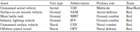


 Open access