

Introduction
The past behaviour of the Antarctic ice sheets is poorly understood because their presence obscures much of the subglacial environment. In contrast, the beds of former mid-latitude ice sheets now lie exposed (e.g. in North America, Patagonia and north-west Europe), and investigations of glacial geomorphology have provided significant insight into past ice sheet extents, fluctuations and, via an understanding of patterns of glacial erosion, former thermal regimes and flow structures. This paradigm of process-based geomorphology, developed by Sugden and colleagues (Sugden & John Reference Sugden and John1976, Sugden Reference Sugden1978, Reference Sugden1989, Sugden et al. Reference Sugden, Balco, Cowdery, Stone and Sass2005, Reference Sugden, Bentley and O’Cofaigh2006), remains at the forefront of glaciological studies. Recently, a new compilation of bed topography beneath Antarctica has been released (Fretwell et al. Reference Fretwell, Pritchard and Vaughan2013; Fig. 1), which adds significant morphological detail to parts of this generally inaccessible landscape. The availability of these data enables exploration of the growth and past behaviour of the Antarctic ice sheet and, in particular, the comparatively less-well studied East Antarctic Ice Sheet (EAIS). Unlike West Antarctica, the much more extensive East Antarctic landscape is tectonically relatively ‘stable’ and largely unmodified by Cenozoic tectonic activity, with potential to preserve a very ancient glacial history.
Antarctic BEDMAP2 topography (Fretwell et al. Reference Fretwell, Pritchard and Vaughan2013) rebounded after the removal of present ice load. The black line indicates the modern grounding line (Scambos et al. Reference Scambos, Haran, Fahnestock, Painter and Bohlander2007) and the white line indicates sea level under rebounded topographic conditions. AP=Antarctic Peninsula, CL=Coats Land, DML=Dronning Maud Land, EL=Enderby Land, EW=Ellsworth-Whitmore block, GSM=Gamburtsev Subglacial Mountains, GVL=George V Land, KL=Kemp Land, LG=Lambert Graben, MBL=Marie Byrd Land, MRL=Mac. Robertson Land, PEL=Princess Elizabeth Land, QML=Queen Mary Land, RB=Recovery Basin, TA=Terre Adélie, TAM=Transantarctic Mountains, TT=Thiel Trough, VSH=Vostok Subglacial Highlands, WIIL=Wilhelm II Land, WL=Wilkes Land.

The aim of this study was to extend the process-based geomorphological classification of Antarctic glacial landscape (Sugden & John Reference Sugden and John1976) to include the previously ignored region currently buried beneath the Antarctic ice sheets. This was done to develop a better understanding of the past behaviour of the ice sheets and the flow regimes associated with their evolution. Our objectives were to: i) extract regional measurements of landscape geometry (morphometry and hypsometry) from BEDMAP2 (BM2) within the areas originally classified by Sugden & John (Reference Sugden and John1976; Fig. 2) to identify whether distinct erosion process signals can be distinguished within BM2 using their topographic characteristics, ii) subdivide the bed dataset into equal areal units and extract hypsometry across the previously unclassified region, and iii) extend the glacio-geomorphological classification to cover subglacial Antarctica by using the regional hypsometries as a training set to classify the subdivided areas based on their morphometric characteristics.
Previous classifications of glacial landscape character for past and present glaciated beds (re-drafted from Sugden Reference Sugden1974, Sugden & John Reference Sugden and John1976, Sugden Reference Sugden1978). a. Antarctica with the mosaic of Antarctica grounding line (Scambos et al. Reference Scambos, Haran, Fahnestock, Painter and Bohlander2007) shown in black. Note that 90% of the landscape could not be characterized (white). b. Greenland. c. Laurentide.

Background and previous work
Antarctic ice sheets and climate evolution
The EAIS grew in a stepwise fashion, initiating at c. 33.7 Ma in response to a reduction in atmospheric CO2 (DeConto & Pollard Reference DeConto and Pollard2003), and then expanding further as the surrounding ocean cooled (Liu et al. Reference Liu, Pagani, Zinniker, DeConto, Huber, Brinkhuis, Shah, Leckie and Pearson2009, Pusz et al. Reference Pusz, Thunell and Miller2011). Its growth reflects the transition of the Earth from a ‘greenhouse’ to an ‘icehouse’ state at the Eocene-Oligocene (EO) climate transition, which spanned c. 300–400 thousand years and is reflected in deep sea benthic foraminiferal records (Katz et al. Reference Katz, Miller, Wright, Wade, Browning, Cramer and Rosenthal2008, Miller et al. Reference Miller, Wright, Katz, Browning, Cramer, Wade and Mizintseva2008, Pusz et al. Reference Pusz, Thunell and Miller2011). The ice sheet initiated upon the highland topographies of Antarctica and expanded to cover the entire continent (DeConto & Pollard Reference DeConto and Pollard2003). Given our previous knowledge of the bed, based largely on broadly spaced radio-echo sounding surveys, it has long been assumed that important East Antarctic inception points were the Gamburtsev Subglacial Mountains (GSM), Dronning Maud Land (DML) and the Transantarctic Mountains (TAM; Fig. 1). However, it is possible that other, yet to be discovered, subglacial mountain blocks may have also acted as minor nucleation points for East Antarctic ice.
Between 33.7 and 14 Ma, local offshore sediment cores and the global benthic oxygen isotope record suggest that the EAIS margin waxed and waned on a scale similar to Pleistocene Northern Hemisphere ice sheet fluctuations (Naish et al. Reference Naish, Woolfe and Barrett2001, Miller et al. Reference Miller, Wright, Katz, Browning, Cramer, Wade and Mizintseva2008) before a potentially more stable continental EAIS was established under a colder climate. Along with modelling studies (DeConto & Pollard Reference DeConto and Pollard2003, Jamieson & Sugden Reference Jamieson and Sugden2008), these records suggest that the contractions and expansions in ice volume were significant (tens of metres of sea level equivalent; Cramer et al. Reference Cramer, Miller, Barrett and Wright2011) and the implication is that the ice margin, at least in East Antarctica, fluctuated considerably in scale (Siegert Reference Siegert2008) and may have retreated significantly inland from the coast on numerous occasions. There is, as yet, no direct record of the scale of these intermediate ice sheets, or any indication of whether the EAIS remained as a single ice mass, or separated into regional ice sheets or alpine glacier systems that covered the topographic highlands.
In West Antarctica, numerical models of ice growth based on modern subglacial topography suggested glaciation at the EO transition was limited in extent (DeConto & Pollard Reference DeConto and Pollard2003) and that the West Antarctic Ice Sheet (WAIS) only grew when further significant cooling occurred at c. 14 Ma (Miller et al. Reference Miller, Wright, Katz, Browning, Cramer, Wade and Mizintseva2008). However, a recent modelling study (Wilson et al. Reference Wilson, Pollard, DeConto, Jamieson and Luyendyk2013), in accordance with limited field data (Ivany et al. Reference Ivany, van Simaeys, Domack and Samson2006), suggested that a full-scale WAIS may have expanded in tandem with the EAIS because the topography, which is largely below sea level today, was once significantly higher and thus more susceptible to accumulation of snow and ice than previously realized (Wilson et al. Reference Wilson, Jamieson, Barrett, Leitchenkov, Gohl and Larter2012).
Geomorphological domains and inferences regarding ice sheet behaviour
Given the lack of direct records for the extent of the EAIS and WAIS over such large periods of time, the scale and nature of these ice sheet fluctuations is not well known. However, an understanding of the behaviour of the former Laurentide Ice Sheet gained through process-based geomorphological interpretation (Sugden Reference Sugden1978), for example, shows the potential for developing knowledge of past ice behaviour by interpreting ‘newly surveyed’ ice sheet beds (Fig. 1). The modern Antarctic ice sheet bed should record the time-transgressive behaviour of the ice sheets in this region because of the erosional fingerprint imposed on the bed (Jamieson & Sugden Reference Jamieson and Sugden2008, Jamieson et al. Reference Jamieson, Sugden and Hulton2010).
Despite the challenges of deciphering the erosional and ice dynamical regime in the interior of Antarctica, a number of studies have made advances, particularly with respect to the EAIS. For example, Perkins (Reference Perkins1984) proposed that the GSM may retain a much older, ‘sharper’, alpine morphology which, it was later suggested, would have been protected beneath cold-based ice (Jamieson & Sugden Reference Jamieson and Sugden2008). Van de Flierdt et al. (Reference Van de Flierdt, Hemming, Goldstein, Gehrels and Cox2008) found that there was only very limited depositional evidence offshore for the erosion of these mountains, indicating that erosion of the GSM was probably minimal since at least 14 Ma. Bo et al. (Reference Bo, Siegert, Mudd, Sugden, Fujita, Cui, Jiang, Tang and Li2009) and Rose et al. (Reference Rose, Ferraccioli, Jamieson, Bell, Corr, Creyts, Braaten, Jordan, Fretwell and Damaske2013) provide more recent support for this hypothesis using high-resolution radar data and concluded that the geometry of the landscape reflects localized ice flow and erosion under restricted glacial conditions dated to at least 14 Ma, and possibly 33.7 Ma or earlier. Similarly, the buried topography of DML is identified as being eroded by localized ice flow to generate cirques and selective overdeepenings that are inconsistent with continental-scale ice sheet flow and thus probably date from the mid-Cenozoic (Näslund Reference Näslund1997). Further afield, Young et al. (Reference Young, Wright, Roberts, Warner, Young, Greenbaum, Schroeder, Holt, Sugden, Blankenship, van Ommen and Siegert2011) identified the presence of fjord-like features incised through an upland massif in Wilkes Land (WL) that reflected a dynamic EAIS during an earlier phase of its flow. Furthermore, Cook et al. (Reference Cook, van de Flierdt and Williams2013) suggested that the Wilkes Subglacial Basin was subject to fluctuating ice margins during the Pliocene, indicating that East Antarctica may have been less stable than previously thought (Sugden Reference Sugden1996).
Landscapes of glacial erosion
The pattern or mode of glacial landscape evolution is controlled by the size of the overlying ice mass, the long-term direction of flow and the temperature at the base of the ice. These are modulated by pre-glacial topography and the underlying geology. Using these principles, Sugden (Reference Sugden1974, Reference Sugden1978) and Sugden & John (Reference Sugden and John1976) made process-based assessments of ice sheet beds in the Northern Hemisphere whereby the geomorphology was interpreted in terms of regimes of alpine glacial erosion, widespread areal scour and selective linear erosion. Glaciologically, these differentiate between i) small-scale valley and ice cap glaciation (alpine landscapes), ii) warm-based topographically-unconstrained ice sheet flow (areal scour), and iii) cold-based ice cover with fast-flowing, warm-based outlets (selective linear erosion). A classification of landscapes of glacial erosion has been attempted for Antarctica (Sugden & John Reference Sugden and John1976) but was restricted to the coast by the limited exposure of the previously eroded ice sheet bed (Fig. 2). Therefore, the majority of the bed of the modern ice sheet has not been interpreted geomorphologically or in terms of palaeo ice dynamics.
Alpine landscapes have sharp peaks and deep, often closely spaced, valleys. They indicate that ice was constrained by topography and erosion was focussed within existing valleys underneath valley glaciers. The glaciers would most probably be polythermal or warm-based and evidence for these former glacial conditions are common in mountain terrains but are also found in the TAM (Fig. 2), DML (Holmlund & Näslund Reference Holmlund and Näslund1994, Näslund Reference Näslund1997), Ellsworth-Whitmore mountains (EW) (Ross et al. Reference Ross, Jordan, Bingham, Corr, Ferraccioli, Le Brocq, Rippin, Wright and Siegert2014), Marie Byrd Land (MBL) (Andrews & LeMasurier Reference Andrews and LeMasurier1973) and more recently in the GSM in the interior of East Antarctica (Bo et al. Reference Bo, Siegert, Mudd, Sugden, Fujita, Cui, Jiang, Tang and Li2009, Rose et al. Reference Rose, Ferraccioli, Jamieson, Bell, Corr, Creyts, Braaten, Jordan, Fretwell and Damaske2013). Focussed erosion can be rapid at the valley floor and can generate characteristic cirque and valley overdeepenings whereby the valley profile is deepened to the extent that a downflow lip is generated.
Landscapes of areal scour are smoothed, low relief landscapes formed by ice flow that is not focussed significantly by topography. On a large scale they are most commonly associated with landscapes buried under thick ice in central zones of ice sheets (Fig. 2), but on smaller scales they are associated with ice flow convergence and streaming ice (Sugden & John Reference Sugden and John1976). Large parts of the bed of the former Laurentide Ice Sheet are scoured, with low relief, streamlined bedforms, some of which indicate the location of former ice streams (Stokes & Clark Reference Stokes and Clark1999). The magnitude of hard-bed erosion under areal scour conditions in Antarctica is probably low (Sugden Reference Sugden1976, Van de Flierdt et al. Reference Van de Flierdt, Hemming, Goldstein, Gehrels and Cox2008, Jamieson et al. Reference Jamieson, Sugden and Hulton2010). If the bed is underlain by soft sediment, it can often appear similar in morphology to either scoured or selectively eroded landscapes (Bingham & Siegert Reference Bingham and Siegert2009) although the rates of sediment transport can be orders of magnitude higher, particularly under streaming ice (Smith et al. Reference Smith, Murray, Nicholls, Makinson, Aoalgeirsdottir, Behar and Vaughan2007).
Landscapes of selective linear erosion are identified by the presence of significant incisions into a landscape, such as glacial troughs. These landscapes are generated where focussed and often rapid erosion under warm-based thick ice occurs adjacent to areas of minimal topographic modification under cold-based thin ice (Sugden Reference Sugden1974, Sugden & John Reference Sugden and John1976). This is often considered to be a function of the existing topography steering ice flow in upland landscapes (Kessler et al. Reference Kessler, Anderson and Briner2008), with the fjord landscapes of Scandinavia or the north-west coast of Scotland being a characteristic product. It is heavily dependent upon the topographic wavelength, and pre-glacial topography, which enables rapid spatial changes in ice thickness and thus sharp boundaries between warm-based erosive and cold-based protective ice. Erosion can be rapid in the base of the characteristic overdeepened troughs but very low to non-existent on adjacent upland plateaus where ice flow is slower, ice is thinner and basal melting is less probable (Stroeven et al. Reference Stroeven, Fabel, Harbor, Hättestrand and Kleman2002). In Antarctica, the landscapes of the Lambert region are selectively eroded, as are parts of DML (Näslund Reference Näslund2001), the Ellsworth Subglacial Highlands (Ross et al. Reference Ross, Jordan, Bingham, Corr, Ferraccioli, Le Brocq, Rippin, Wright and Siegert2014), MBL (Sugden et al. Reference Sugden, Balco, Cowdery, Stone and Sass2005) and parts of the TAM (Sugden & Denton Reference Sugden and Denton2004, Stern et al. Reference Stern, Baxter and Barrett2005).
Approach and methods
In order to identify the geomorphic and dynamic signal of past Antarctic ice sheet behaviour that is recorded in the BM2 bed elevation dataset, its geometry was analysed and the potential modes of landscape evolution with respect to ice sheet dynamics were interpreted. Although the spatial resolution of the dataset is 1 km, in reality the bed data are interpolated from 5-km spaced data and, therefore, cannot resolve bed features <5 km in size; 64% of the 5-km cells contain no direct measurement. A full discussion of data coverage and limitations can be found in Fretwell et al. (Reference Fretwell, Pritchard and Vaughan2013).
The BM2 dataset was isostatically adjusted to account for the removal of the modern ice sheet load and provide a basis for comparison to beds of former ice sheets in the Northern Hemisphere. Following Wilson et al. (Reference Wilson, Jamieson, Barrett, Leitchenkov, Gohl and Larter2012), the isostatic model calculates flexural load assuming a thin elastic plate with a uniform effective elastic thickness of 35 km overlying a non-viscous fluid. The load of water that replaces ice in areas that lie below sea level is iteratively calculated and applied to the ice-free landscape until, for reasons of computational efficiency, the load change drops below c. 2 m in magnitude. The water loading incorporates a uniform eustatic sea level rise of 60 m that represents the addition of Antarctic ice to the ocean but that does not account for spherical earth or gravitational effects. The relaxed topography (BM2r) is shown in Fig. 1 and in the supplementary material (http://dx.doi.org/10.1017/S0954102014000212).
Morphometric analysis and modes of glacial landscape evolution
Morphometric analysis characterizes the topography of a digital elevation model and enables the identification of particular landscape types, thus, linking a landscape to its genesis and evolution. In terms of ice sheet beds, this is a natural extension of the process-based geomorphological approach pioneered by Sugden et al. The hydrology and surface toolboxes from the ArcGIS spatial analyst extension (ESRI 2012), and the peak classification tool from Landserf (Wood Reference Wood2005), were used to extract a series of morphometric measurements from BM2r including hypsometry, relief, peak characteristics, basins and drainage form.
Hypsometry describes the percentage distribution of landscape area against elevation, which can be linked to the process of landscape evolution and has been applied to parts of the bed of Antarctica (Rose et al. Reference Rose, Ferraccioli, Jamieson, Bell, Corr, Creyts, Braaten, Jordan, Fretwell and Damaske2013). It records the shape of the land surface. However, different processes may result in similar histograms within low-resolution data making it most useful when applied in conjunction with other physical measures of landscape. Descriptive statistics, including measures of skewness and kurtosis, were also extracted. If a histogram is not bimodal, negative skewness indicates that the lower elevation tail is either longer or fatter than the higher elevation tail, and positive values indicate the higher elevation tail is longer or fatter. Thus, negative skew indicates that the mode of the areal distribution lies at higher relative elevation, but that the mean of its distribution lies below this value. Therefore, negative skewness is indicative of enhanced area at higher elevation. Kurtosis describes the ‘peakedness’ of the histogram. A normal distribution has a kurtosis of three, with values below this indicating a lower, flatter peak to the area-elevation distribution, such as in a landscape with uniform slope angles. High kurtosis indicates a significant percentage of the landscape area lies in a narrow elevation band.
The locations of individual ‘peaks’ of at least 1000, 2000, 3000 or 4000 m elevation that rise 250 m clear of any adjacent peaks were extracted. These peaks are simply high points in the BM2r dataset and describe average elevations over a 5-km grid area. As a consequence they provide minimum estimates for the density of actual peaks. The density of individual peaks is higher in a landscape dominated by alpine glacial erosion compared to one where topography is submerged beneath an ice sheet over a much greater area and where peaks can, therefore, be potentially subject to modification. Peak heights were also measured, which indicates the scale of mountainous terrain. Furthermore, it has often been noted that pre-glacial landscapes and saprolites that become incised under ice sheets can be partly preserved as remnants in glaciated landscapes (Sugden Reference Sugden1989, Hättestrand & Stroeven Reference Hättestrand and Stroeven2002, Goodfellow Reference Goodfellow2007). Therefore, consistency in peak heights may evince the presence of remnants of pre-glacial landsurfaces that have subsequently been incised by surface processes.
The elevation range (relief) and slopes within each unit of the landscape were calculated and may help identify whether the topography has been selectively eroded or whether it has been smoothed. Relief may also help identify whether the landscape has been subjected to long-term flow that has not significantly changed direction and has, therefore, had longer to incise the landscape. Within this context, and at a kilometre scale, relatively low slopes with little variation may be expected in zones of areal scour whereas a bimodal distribution of very low and very high slopes might indicate a selectively eroded fjord-like landscape.
The large-scale valley drainage network was also extracted because this has previously been used as an indicator of processes related to long-term Antarctic landscape evolution (Baroni et al. Reference Baroni, Noti, Ciccacci, Righini and Salvatore2005, Jamieson et al. Reference Jamieson, Hulton, Sugden, Payne and Taylor2005). For example, a dendritic network may be an indicator of an unperturbed drainage system whereas deviation from this may indicate structural control or modification of valley spacing by erosion processes operating on a different scale to the fluvial system. The network was extracted by assuming that the rivers would be routed down the steepest slope within the landscape. Drainage was deliberately extracted to the edge of the modern grounded ice in order to understand the potential impact of glacial processes upon the bed, but the coastline would have lain inland of this position during ice-free conditions. Where internal basins are present, these were filled to enable drainage to the coast from all basins. The valley network and the associated internal basins are an indicator not only of water flow, but of sediment transport pathways and depo-centres during periods when parts of the bed topography lie exposed.
Morphometric analysis of BEDMAP2r
In addition to the measurement of the ice sheet bed topography, and in order to conduct a process-based geomorphological classification of the Antarctic subglacial landscape, specific regions of the BM2r database that relate to Sugden & John’s (Reference Sugden and John1976) original classification were also characterized (Fig. 2). This was done in two phases. First, the characteristics of the sub-aerial regions previously classified by Sugden & John (Reference Sugden and John1976; Fig. 2) were analysed to establish whether the morphometric analysis enables discrimination of distinct morphological characteristics for each landscape type. Crucially, the density of point measurements within BM2 is high in these areas. Second, using the same methods, the entirety of BM2r was analysed, applying the analysis in a grid of equally divided regions. Normally, hypsometry and other morphometric parameters would be determined using individual drainage basins as the areal unit of interrogation. However, the scale of the basins in Antarctica is such that some encompass regions where the ice margin might be expected to have fluctuated and, therefore, might show a mixed signal of landscape evolution. Consequently, BM2r is divided into a regular 250×250 km grid to provide standardized units for comparison across the bed. The use of this areal division allows direct comparison to regions in the earlier classification and provides a higher resolution analysis than is possible using drainage basin extents.
Following the extraction of these data, the morphometry of the original classifications (Fig. 2; Sugden & John Reference Sugden and John1976) was used as training data to characterize the glaciological processes that generated the landscapes of the previously unclassified regions. Two extended classifications have been produced. The first relies strictly upon the previously classified training set, and follows a simple decision pathway to expand the classification into the centre of East and West Antarctica. The second is more tentative, using the first classification to direct a higher-resolution categorization. In generating the latter classification, our understanding of the long-term thermal structure drives the decisions. In particular, it is possible that rapid expansion from alpine scale to ice sheet scale glaciation occurred in Antarctica and, therefore, a protective cold-based ice sheet core established over the alpine landscape and preserved it under continental scale ice flow conditions (Jamieson et al. Reference Jamieson, Hulton and Hagdorn2008, Bo et al. Reference Bo, Siegert, Mudd, Sugden, Fujita, Cui, Jiang, Tang and Li2009, Jamieson et al. Reference Jamieson, Sugden and Hulton2010, Rose et al. Reference Rose, Ferraccioli, Jamieson, Bell, Corr, Creyts, Braaten, Jordan, Fretwell and Damaske2013). The assumption was transferred that this scale of selectivity may have been possible where steep topography and, thus, thermal gradient enabled cold-based ice to encase whole alpine landscapes rather than just upland plateaus. Thus, alpine landscapes can be nested within selectively eroded landscapes, as seen in the Ellsworth Subglacial Highlands (Ross et al. Reference Ross, Jordan, Bingham, Corr, Ferraccioli, Le Brocq, Rippin, Wright and Siegert2014), and these are delineated based upon the identification of regions of high elevation that also have a ‘rough’ appearance. Our intention is that this new classification be treated as a working hypothesis for the modes of landscape evolution in Antarctica.
Results
The drainage network of Antarctica
The drainage network, drainage divides and the probable internal sediment depo-centres are shown in Fig. 3. The numerous numerically-filled basins partially mask channel morphology by generating multiple parallel channels across the erroneously flattened topography. This makes detailed network analysis, such as calculation of bifurcation ratios, drainage density and Horton numbers, which can all identify divergence from a dendritic morphology, subject to significant potential error. Therefore, note that in East Antarctica the river network is largely dendritic in appearance and drains radially from the GSM and Vostok Subglacial Highlands (VSH). Indeed, the six largest drainage basins in East Antarctica are all similar in length (1400–1780 km), radiating from their relatively confined headwater region. Behind the TAM, drainage is directed towards the interior before draining longitudinally for up to 1500 km towards the coast of George V Land (GVL) or through the Thiel Trough (TT) into the Weddell Sea.
Drainage network on the BM2r landscape. a. Deglacial hydrological and sediment transport pathways. The drainage pattern is dendritic in appearance and drains radially. b. The depth of potential depo-centres in the deglaciated BM2r and the location of modern subglacial lakes. Topography is shown using a hillshade of BM2r. The mosaic of Antarctica grounding line (Scambos et al. Reference Scambos, Haran, Fahnestock, Painter and Bohlander2007) is shown in black in both panels.

The presence of coastal highlands between 100°E and 15°W results in the development of small, locally draining basins indicating that short-scale (100–300 km distance) fluvial sediment delivery would be probable. On the inland flanks of these highlands, drainage is oriented towards the continental interior before draining longitudinally towards the coast. Valley spacing in the TAM is similar to that in the remaining coastal highlands. However, in WL, Terre Adélie (TA) and GVL, such small-scale drainage is less dominant, with longer drainage pathways extending from the interior out to the coast in a radial, dendritic manner. The potential depo-centres (and thus lakes during ice free periods) are largely located inland of the coastal mountain ranges and are all interconnected via the drainage network. In Coats Land (CL), WL and GVL, the depo-centres are relatively larger, less frequent and appear to be aligned to existing ice sheet flow. However, in the remainder of East Antarctica the alignment is less obvious, with larger numbers of smaller basins. In West Antarctica, the largest depo-centres and much of the drainage are aligned along the path of ice sheet flow but would lie below sea level whether ice free or not (Figs 1 & 3). In the Antarctic Peninsula (AP), the drainage basins are short with the longitudinal drainage divide located approximately equidistant from the west and east coasts.
The distribution of mountainous terrain in Antarctica
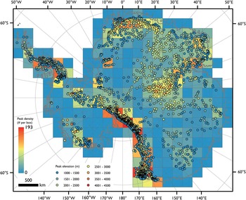
Following on from the identification of the low points in the landscape and the ice sheet wide drainage networks, the distribution of independent 1000 m peaks in the BM2r dataset is shown in Fig. 4. They are located most commonly in the alpine regions of the TAM, MBL and the AP. They are also found along coastal regions of East Antarctica stretching from DML to the Lambert region. In the interior, only the GSM show significant ‘peak’ densities, although other smaller clusters of 1000 m peaks are found in the interior of East Antarctica. These latter groups may hint at sharp, mountainous landscapes, like the GSM, that are poorly resolved beneath the ice.
Distribution of 1000 m ‘peaks’ (which describe an area of high elevation averaged over a 5×5 km region) and peak density in BM2r. Peaks that are >1000 m in elevation and that lie 250 m proud of surrounding topography are indicated by a point. Peak densities are shown for each analysis box. The mosaic of Antarctica grounding line (Scambos et al. Reference Scambos, Haran, Fahnestock, Painter and Bohlander2007) is shown in grey.
The morphometry of Antarctica’s eroded landscapes
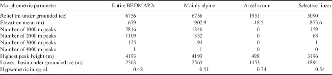
The topographic data for the three subsets of landscape classification and for BM2r as a whole are shown in Table I.
Key morphometric parameters extracted from BM2r across previously classified parts of the landscape and across the entire currently grounded portion of the dataset.
Hypsometries for the classified regions are shown in Fig. 5 alongside similar data for portions of exposed ice sheet beds in the Northern Hemisphere. The mainly alpine region displays a broad elevation distribution and unimodal, near-normal distribution similar to the European Alps. The region of areal scour has a narrow elevation range within which the majority of the landsurface is distributed at relatively low altitude. The selective linearly eroded landscape displays a bimodal distribution indicating incision of flat-bottomed troughs into upland plateau topography. The spacing between peaks in the bimodal distribution suggests an average trough depth of c. 1 km.
Hypsometric (area-elevation) relationships of the rebounded Antarctic bed within previously identified landscapes of erosion. Inset: hypsometric curves for parts of former ice sheet beds extracted from GMTED 15 arc-second resolution data (USGS 2010): alpine topography in the European Alps, glacially scoured topography to the west of Hudson Bay (Canada), and selectively eroded topography in the north-west draining part of Baffin Island.

The classified regions (Fig. 2) have distinctive morphologies, in particular in the hypsometric distributions. The mainly alpine region has a high regional relief of 6756 m, with a near-normal area-elevation distribution (Fig. 5). The drainage network, and thus valley network, in this region is closely spaced across flow and the drainage areas are small with short trunk rivers whose headwaters are enclosed by the region. The density of peaks >1000 m in relief is eight times higher than in any other region (Fig. 4), although due to restricted data coverage it would be improbable that comparably high densities could be picked out in the subglacial region of Antarctica if alpine landscapes do exist.
The selective linear erosion region (Fig. 2) has a high relief (5090 m) and mean elevation of 874 m, but also a bimodal hypsometric distribution indicating the dominance of upland plateaus and glacially eroded valley floors in the landscape. Significant independent peaks are less common than in alpine regions (Fig. 4) and drainage appears to be routed through the valley floors from areas further inland (Fig. 3).
The regions of areal scour (Fig. 2), though limited in coverage, show that relief is <2000 m with a mean elevation closer to sea level. The scoured landscapes do not contain significant independent peaks and have not had deep valleys carved into them. The drainage network (Fig. 3) indicates that the headwaters of the rivers lie inland and cross the scoured topography en-route to the coast. However, regions of extensive deposition may have similar landscape geometries to those of areal scour. For example, areas outboard of the 0 m contour (Fig. 1), where marine sedimentation is most probable, are the regions where deposition may mask earlier patterns of glacial erosion.
Expanding the Sugden & John classification of glacial landscape evolution
The hypsometries for each boxed region of the BM2r dataset are extracted (Fig. S1) and the morphometric parameters are outlined in Table S1 (supplementary material will be found at http://dx.doi.org/10.1017/S0954102014000212). In order to show how the ‘boxed’ morphometric analysis would extend the Sugden & John (Reference Sugden and John1976) classification (Fig. 2), a simple decision pathway was applied (Fig. 6) based on the regional morphometric analysis and each box was assigned to one of the original classes. Criteria were applied in order of significance, building the assessment of each region by applying additional criteria one at a time until the area fitted into a single category. The minimum discriminators of hypsometric distribution and then relief were applied because these encompass the form and scale of the topography in single measurements. Thereafter, mean slope, peak density and drainage density were applied if the classification remained ambiguous. The chosen values overlap for some of the criteria, but a unique answer was reached when all were applied. The hypsometries were extracted and then coloured according to this decision pathway (Fig. 7).
Decision pathway used to determine landscape classification within box regions of BM2r. Y=yes, N=no.

Antarctic hypsometry within each box region (Fig. S1). For each graph, y-axis=area, x-axis=elevation. The maximum and minimum elevations shown in each graph are presented in Table S1. The histograms are coloured following the application of the ‘training dataset’ to the morphometry and hypsometry of each square region. Greyed boxes highlight regions within BEDMAP2 where >50% of the area of the bed has been generated from data that is >200 km distant (see fig. 3 in Fretwell et al. Reference Fretwell, Pritchard and Vaughan2013). The mosaic of Antarctica grounding line (Scambos et al. Reference Scambos, Haran, Fahnestock, Painter and Bohlander2007) is shown in grey. Table S1 and Fig. S1 will be found at http://dx.doi.org/10.1017/S0954102014000212.

As Fig. 7 illustrates, there is significant variability in the signal of glacial landscape evolution. In general, landscapes of selective erosion tend to be found in pathways leading from the interior to the coast or as a more localized signal in the coastal mountains. Landscapes of selective erosion, including areas where sedimentary drapes have probably eroded, seem to underlie much of the present WAIS. Zones of alpine morphology are often narrow in width and occur, as might be expected, along the TAM, in DML, MBL, in the GSM and along the AP. Small areas of alpine morphology are also picked out corresponding to the Ellsworth Mountains and inland of the Amundsen and Bellingshausen seas. Areal scour is widespread in the interior, particularly in East Antarctica, and is found in the regions that lie between alpine landscapes or in areas where topography is comparatively low in relief. There are only small zones of areal scour in West Antarctica. However, within the BM2 there are regions where there are hundreds of km between bed measurements and thus where topography may appear smoother than it is in reality (Fig. 1). Areas where data quality may have a significant impact upon the classification of the landscape are highlighted on Fig. 7 by grey shading.
The boxed morphometric classification provides a low-resolution template for a second, finer-scale, qualitative classification (Fig. 8). The key result of this is the significantly expanded coverage of mainly alpine landscape; preserved alpine landscapes may be much more commonplace under the Antarctic ice sheets than previously realized, particularly beneath the EAIS. For example, the region inland of the coastal mountains of DML is extended and reaches towards the mainly alpine GSM, which are also extended beyond previous knowledge. Although smaller in extent, isolated alpine ranges may also be found throughout the region between Dome C and the coast, and in Enderby Land (EL). The VSH are also picked out as being potentially alpine, as are inter-ice stream regions in the Recovery Basin (RB). The TAM and core of the AP and MBL highlands are also mainly alpine, as is most of the Ellsworth-Whitmore region. As selective erosion occurs under continental-scale ice, flow-parallel alpine chains may have been preserved in Coates Land (CL) and the RB.
Zones of areal scour are delineated in coastal areas of CL, DML, Princess Elizabeth Land (PEL), Wilhelm II Land (WIIL), Queen Mary Land (QML) and TA where topography is relatively smooth and is not topographically confined at a small scale. Scour is also suggested to be found under the South Pole, in a region between Dome C and the VSH, and between the alpine topographies of DML and the GSM. In these three cases, the areas of scour are surrounded by alpine topography and are, therefore, defined by zones where ice flow direction under smaller-scale ice may have been significantly different from flow direction under continental-scale ice.
Selective linear erosion is used to describe the remainder of the landscape. It effectively radiates from the alpine centres and occupies zones through which continental-scale ice has, or still, drains to the coast. It is also picked out on the range fronts of DML, the TAM and in the AP where overdeepened trough features reach to sea level. The bed of much of West Antarctica is also indicated to be selectively eroded although our analysis does not directly distinguish parts of the WAIS bed that have been strongly affected by tectonic processes or marine sedimentation.
Discussion
Geomorphic interpretation of past Antarctic ice dynamics
Many of the alpine landscapes correspond to regions which, under the modern ice sheet, are thought to have high basal-friction coefficients and thus low rates of basal sliding (Morlighem et al. Reference Morlighem, Seroussi, Larour and Rignot2013). Consistent with modelling studies for Antarctica (Jamieson & Sugden Reference Jamieson and Sugden2008, Jamieson et al. Reference Jamieson, Sugden and Hulton2010, Golledge et al. Reference Golledge, Levy, McKay, Fogwill, White, Graham, Smith, Hillenbrand, Licht, Denton, Ackert, Maas and Hall2013), and with geomorphological studies from Northern Hemisphere ice sheet beds (Kleman Reference Kleman1994, Kleman & Stroeven Reference Kleman and Stroeven1997), the implication is that these regions are subject to little or no erosion and, therefore, favour large-scale preservation of alpine landscapes. Remarkably, the logical extension of this model for preservation is that in these areas the cold-base of the overlying ice sheet must have remained unchanged despite evolving through c. 58 glacial cycles during the last 13 million years (McKay et al. Reference McKay, Browne, Carter, Cowan, Dunbar, Krissek, Naish, Powell, Reed, Talarico and Wilch2009). This is consistent with investigations of probable sites for the discovery of ice older than 1 million years (Van Liefferinge & Pattyn Reference Van Liefferinge and Pattyn2013). However, as a result of our analysis, we hypothesize that these cold-based regions may be more extensive in DML as indicated by the distribution of peaks, and thus rougher topography, in this area (Fig. 4).
The alpine landscapes reflect restricted previous ice extents which had topographically confined radial flow and a largely warm basal thermal regime. However, as the scale of valley and peak spacing is inconsistent with continental patterns of ice flow, many of the currently buried and preserved landscapes are probably ancient (Jamieson & Sugden Reference Jamieson and Sugden2008, Siegert Reference Siegert2008, Rose et al. Reference Rose, Ferraccioli, Jamieson, Bell, Corr, Creyts, Braaten, Jordan, Fretwell and Damaske2013). It is probable that all the alpine landscapes are time-transgressive. For example, an equilibrium-line altitude (ELA) that intersects the topography at 2000 m elevation would have enabled ice growth in the TAM, AP, MBL, GSM, VSH and DML but it would have to have been depressed by another 500–800 m to enable valley glaciers to grow in the more isolated alpine areas between the coast and the GSM. During such a drop in ELA, ice in the initially glaciated regions would probably have advanced and coalesced into mountain ice caps or regional ice sheets (Jamieson et al. Reference Jamieson, Sugden and Hulton2010). Therefore, although there is evidence for warm-based valley glaciation in a number of areas near the coast since the expansion of the continental ice sheet (Holmlund & Näslund Reference Holmlund and Näslund1994, Armienti & Baroni Reference Armienti and Baroni1999, Di Nicola et al. Reference Di Nicola, Baroni, Strasky, Salvatore, Schlüchter, Akçar, Kubik and Wieler2012), it is possible that the larger alpine domains (e.g. GSM and VSH) were last incised by valley glaciers before 14 Ma and that the ice masses that fluctuated between 33.7 and 14 Ma may never have retreated as far as these interior alpine systems. Thus, although it cannot be confirmed, it is also a possibility that they could represent sites eroded during the initiation of the EAIS at 33.7 Ma. This gives rise to the scenario that the distribution of potential sites for initial ice growth, at least in East Antarctica, may be broader than previously realized (DeConto & Pollard Reference DeConto and Pollard2003, Jamieson & Sugden Reference Jamieson and Sugden2008).
To find landscapes of selective linear erosion in the interior of a glaciated terrain is unusual because the process relies upon ice being thin enough to preserve parts of the landscape whilst being thicker in existing depressions such that ice can be warm-based and erosive. However, the unique nature of Antarctic glaciation allows the ice sheet margins to fluctuate significantly over an extended period of time (Naish et al. Reference Naish, Woolfe and Barrett2001, DeConto & Pollard Reference DeConto and Pollard2003). Although the positions of ice margins are not constrained, it is probable that under smaller, regional-scale ice sheets, ice in the interior of the continent would be thinner and thus more sensitive to topographically-driven contrasts in basal thermal regime and enhanced selectivity than would be the case under a continental ice sheet. Therefore, the presence of selectively eroded landscapes suggests that, in the past, ice was thin enough to erode selectively, and that margins probably retreated inland of the coast. At present, these areas are often buried under thick, slow flowing ice that is less liable to significantly erode. Furthermore, the presence of a sedimentary drape, such as that noted in West Antarctica during recent surveys (Bingham & Siegert Reference Bingham and Siegert2009, Ross et al. Reference Ross, Bingham, Corr, Ferraccioli, Jordan, Le Brocq, Rippin, Young, Blankenship and Siegert2012), may alter patterns of hard bed erosion and mask the past signal of erosion by smoothing the bed landscape.
We identified a number of areas in the interior where alpine landscapes are inset within selective linear erosion landscapes whose orientations are inconsistent with continental ice flow. These include areas inboard of EL and the interior of WL and QML. In these cases, the landscape may be preserving at least two scales of ice behaviour prior to the onset of full glaciation. For example, Young et al. (Reference Young, Wright, Roberts, Warner, Young, Greenbaum, Schroeder, Holt, Sugden, Blankenship, van Ommen and Siegert2011) identified a fjord landscape in QML indicative of a dynamic early ice sheet; we propose that a contemporaneous or earlier alpine landscape may have been eroded and selectively preserved in the uplands between the fjords.
Furthermore, the preservation of pre-glacial landscape remnants is most probable where the direction of ice flow under a selective erosion regime remains constant under both a regional- and a continental-scale ice sheet. Examples of pre-glacial landscape preservation include Scandinavia (Kleman & Stroeven Reference Kleman and Stroeven1997, Hättestrand & Stroeven Reference Hättestrand and Stroeven2002), DML (Näslund Reference Näslund1997) and Scotland (Sugden Reference Sugden1989) all of which have pre-glacial landscape remnants that often lie at similar elevations over large areas and are separated by sharp boundaries such as trough walls (Goodfellow Reference Goodfellow2007). The selectively eroded landscape between the GSM and the Lambert trough may contain such landscape fragments. This is identified by the relatively consistent elevation of peak heights in this area. Here, convergent, topographically steered ice flow patterns have probably been consistent since the onset of East Antarctic glaciation. Drainage from the GSM to the Lambert region was established early and significant change during periods of either expanded or reduced ice sheet extent is doubtful (Jamieson et al. Reference Jamieson, Hulton, Sugden, Payne and Taylor2005). This pattern of flow has led to significant incision and erosion-driven uplift on the flanks of the Lambert Graben (Lisker et al. Reference Lisker, Brown and Fabel2003), particularly between 34 and 24 Ma (Tochilin et al. Reference Tochilin, Reiners, Thomson, Gehrels, Hemming and Pierce2012, Thomson et al. Reference Thomson, Reiners, Hemming and Gehrels2013). We suggest that the uplift between the GSM and the Lambert Graben caused an increasingly selective basal thermal regime to evolve whereby thick warmer ice in trough floors became warmer, and thin colder ice on peaks became colder. This would enhance the likelihood of maintaining cold-based ice over the pre-glacial topography fragments and is consistent with generating the crustal upwarping noted by Ferraccioli et al. (Reference Ferraccioli, Finn, Jordan, Bell, Anderson and Damaske2011).
The age of subglacial landscapes
Our knowledge of the scale and timing of ice sheet fluctuations remains limited, as does the impact and scale of tectonically-driven changes to landscape and ice flow. The evolution of different scales of glacial erosion is time-transgressive. Therefore, we have built on work by Siegert (Reference Siegert2008) and Jamieson & Sugden (Reference Jamieson and Sugden2008) to suggest broad scenarios for the ages of the eroded and protected glacial landscapes. For example, before 33.7 Ma, local, warm-based, ephemeral alpine glaciers eroded the highest elevation coastal and interior highlands of East Antarctica, and possibly the AP and the highlands of West Antarctica depending on their elevation (e.g. Wilson et al. Reference Wilson, Pollard, DeConto, Jamieson and Luyendyk2013).
The period between 33.7 and 14 Ma would have supported a significant range of erosion configurations depending on the scale of cyclical margin advance and retreat. Under restricted ice conditions, alpine glaciers would erode and deposit at high elevation in the coastal and interior mountains of East Antarctica, such as DML, VSH, GSM and the TAM, as well as in the highlands of West Antarctica. Under regional ice conditions, alpine erosion would occur in lower elevation mountain blocks (including in EL, RB, QML and TA), whilst over the coastal and interior highlands, larger ice caps or ice sheets would selectively erode pre-existing valleys in a radial pattern. The highest parts of the mountains could have been protected under thin, cold-based ice. Depending upon the elevation and pre-existing valley orientations of West Antarctica, significant ice domes could have been present, radially and selectively eroding the landscape. During the periods when regional ice masses coalesced to become continental-scale ice, alpine glacial erosion would have been more limited. Instead, a mix of continentally or regionally radial selective linear erosion and areal scour would have occurred in East and West Antarctica at, and since, the EO transition (Ehrmann & Mackensen Reference Ehrmann and Mackensen1992, Naish et al. Reference Naish, Woolfe and Barrett2001, Ivany et al. Reference Ivany, van Simaeys, Domack and Samson2006). Such warm-based ice sheets have also deposited sediment multiple times and at many sites in East Antarctica (Webb et al. Reference Webb, Harwood, Mabin and McKelvey1996, Hambrey & McKelvey Reference Hambrey and McKelvey2000, Baroni et al. Reference Baroni, Fasano, Giorgetti, Salvatore and Ribecai2008). Selective erosion would be most prevalent near the coast of East Antarctica where local relief could exert the greatest control of ice drainage and basal thermal regime. If the ice margin were near the coast, extensive regions of cold-based, protective ice would occur over high-elevation mountain peaks and plateaus.
Since 14 Ma, alpine glacial erosion would have been largely restricted to the AP, and to coastal mountain ranges depending on the scale of ice-margin fluctuations (McKay et al. Reference McKay, Browne, Carter, Cowan, Dunbar, Krissek, Naish, Powell, Reed, Talarico and Wilch2009). However, in East Antarctica, it is possible that the large alpine domains in the interior have been preserved under a relatively stable and cold basal thermal regime for 12–14 million years or longer (Bo et al. Reference Bo, Siegert, Mudd, Sugden, Fujita, Cui, Jiang, Tang and Li2009, Rose et al. Reference Rose, Ferraccioli, Jamieson, Bell, Corr, Creyts, Braaten, Jordan, Fretwell and Damaske2013). This is unlikely towards the coast where valley glaciers were last eroding at between 8.2 and 7.5 Ma in the northern Victoria Land sector of the TAM (Armienti & Baroni Reference Armienti and Baroni1999, Di Nicola et al. Reference Di Nicola, Baroni, Strasky, Salvatore, Schlüchter, Akçar, Kubik and Wieler2012) and until 2.5 Ma in DML (Holmlund & Näslund Reference Holmlund and Näslund1994). Notwithstanding the potential for alpine-scale ice to erode intermittently, given the cold polar climate and generally large-scale ice sheets, continental-scale selective linear erosion and areal scour probably dominated in both East and West Antarctica. In the TAM and Mac. Robertson Land (MRL) this selectivity has driven significant uplift in a response to erosional unloading (Stern et al. Reference Stern, Baxter and Barrett2005, Tochilin et al. Reference Tochilin, Reiners, Thomson, Gehrels, Hemming and Pierce2012, Thomson et al. Reference Thomson, Reiners, Hemming and Gehrels2013), although in the TAM, little of this uplift occurred after 3 Ma (Brook et al. Reference Brook, Brown, Kurz, Ackert, Raisbeck and Yiou1995). The area covered by protective, cold-based ice would have been largest during this period, selectively covering mountain plateau tops on a large-scale in the East Antarctic interior, and to a lesser extent over lower elevation mountain ridges and plateaus. The transition into this thermal state may have been rapid in the interior of the continent, as suggested by the lack of ice sheet scale modification to areas like the GSM (Rose et al. Reference Rose, Ferraccioli, Jamieson, Bell, Corr, Creyts, Braaten, Jordan, Fretwell and Damaske2013), but slower towards the coast (Armienti & Baroni Reference Armienti and Baroni1999). The stable hyper-arid polar climate means that preserved, or only slightly modified landscapes, are also found beyond the ice margin (e.g. Baroni et al. Reference Baroni, Noti, Ciccacci, Righini and Salvatore2005, Di Nicola et al. Reference Di Nicola, Baroni, Strasky, Salvatore, Schlüchter, Akçar, Kubik and Wieler2012) or above the ice surface (e.g. Näslund Reference Näslund2001). If, as is hypothesized, the Pliocene WAIS collapsed between 5 and 3 Ma (McKay et al. Reference McKay, Browne, Carter, Cowan, Dunbar, Krissek, Naish, Powell, Reed, Talarico and Wilch2009), then radially selective ice flow from the remaining isolated ice domes would have prevailed, and these would probably retain small cores of thin, cold-based ice.
Throughout these periods, if erosion has been selective or topographically confined, there is potential for an evolving feedback between topography, tectonics, ice flow and erosion. Although we have not explicitly accounted for tectonic processes in our analysis of the subglacial landscape, it is important to note that erosion patterns could either be enhanced or muted over time depending on the direction and scale of any active tectonic uplift or lithospheric subsidence.
Erosion and its influence upon ice behaviour
The dendritic nature of the drainage network, particularly in East Antarctica (Fig. 3), is an indicator that, although glacial erosion has modified the landscape, on a large scale the fluvial network has probably been retained and selectively exploited by glacial erosion. The pre-glacial drainage network itself is controlled by the influence of tectonics because selective erosion around the coast, for example in the TAM, corresponds closely with the valley spacing generated during passive margin uplift following continental separation (Näslund Reference Näslund2001, Stern et al. Reference Stern, Baxter and Barrett2005, Jamieson & Sugden Reference Jamieson and Sugden2008). Furthermore, although the central TAM uplifted in response to episodic tectonic events during the Cretaceous and Cenozoic (Fitzgerald & Stump Reference Fitzgerald and Stump1997), models predict that 32–50% of the peak elevation may have been a response to lithospheric unloading by selective linear erosion (Stern et al. Reference Stern, Baxter and Barrett2005). This may have acted to ensure erosion was increasingly focussed along consistent flow lines, and shows that the interaction between TAM uplift and trough incision is important for ice sheet behaviour (Kerr & Huybrechts Reference Kerr and Huybrechts1999). Large-scale tectonic features have also controlled and re-enforced the ice flow, and therefore erosion, patterns across Antarctica (Jamieson et al. Reference Jamieson, Hulton, Sugden, Payne and Taylor2005, Jamieson & Sugden Reference Jamieson and Sugden2008). For example, in the Lambert basin of MRL, 1.6–2.5 km of selective erosion during the early Oligocene was focussed along the pre-existing graben and resulted in significant uplift of the Prince Charles Mountains in response to the removal of material (Tochilin et al. Reference Tochilin, Reiners, Thomson, Gehrels, Hemming and Pierce2012, Thomson et al. Reference Thomson, Reiners, Hemming and Gehrels2013). The importance of tectonic features is also indicated by the scale of the longitudinal drainage routing behind the TAM, which is similar to the Indus and Brahmaputra river systems which follow the structural grain of the Himalaya for thousands of kilometres before turning to the coast. In many cases, the internal basins correspond to present, and probably former, subglacial lake locations (Fig. 3), and are often situated in rift basins (Ferraccioli et al. Reference Ferraccioli, Jones, Curtis and Leat2005, Reference Ferraccioli, Finn, Jordan, Bell, Anderson and Damaske2011, Jordan et al. Reference Jordan, Ferraccioli, Vaughan, Holt, Corr, Blankenship and Diehl2010, Reference Jordan, Ferraccioli, Armadillo and Bozzo2013, Bingham et al. Reference Bingham, Ferraccioli, King, Larter, Pritchard, Smith and Vaughan2012) or may correspond to overdeepenings eroded by ice (Rose et al. Reference Rose, Ferraccioli, Jamieson, Bell, Corr, Creyts, Braaten, Jordan, Fretwell and Damaske2013, Ross et al. Reference Ross, Jordan, Bingham, Corr, Ferraccioli, Le Brocq, Rippin, Wright and Siegert2014). Thus, via selective erosion, the pre-glacial tectonically-controlled river drainage may have become increasingly important for steering regional ice flow. Furthermore, in places, these depo-centres may contain sedimentary drapes emplaced by marine sedimentation at times when the ice sheet was less extensive (Ross et al. Reference Ross, Bingham, Corr, Ferraccioli, Jordan, Le Brocq, Rippin, Young, Blankenship and Siegert2012).
The importance of topographic feedbacks in controlling ice behaviour extends further. When comparing our classification (Fig. 8) to reconstructions of basal friction (Morlighem et al. Reference Morlighem, Seroussi, Larour and Rignot2013), on a broad scale, the mainly alpine regions correspond with high friction, areal scour with intermediate friction, and selective linear erosion with lower friction. This is consistent with previous analyses indicating that smoother regions of the bed tend to correspond with areas of faster flow (Rippin et al. Reference Rippin, Bamber, Siegert, Vaughan and Corr2004, Siegert et al. Reference Siegert, Taylor and Payne2005, Bingham & Siegert Reference Bingham and Siegert2009). Thus, in a system eroding into bedrock, a topographically-controlled feedback can be envisaged whereby smooth beds may be eroded over time to become more streamlined and thus more efficient in terms of ice drainage; i.e. smooth topography promotes fast flow, which promotes further smoothing (Rippin et al. Reference Rippin, Vaughan and Corr2011). Conversely, the rugged nature of alpine topographies preserved beneath the ice sheet means that ice flow cannot be fast, that ice will probably remain cold-based and that subglacial topographic gradients are often in different directions to continental-scale ice surface gradients. Thus, rough topography may enhance its own preservation potential.
The erosion of glacier and ice sheet beds to elevations below sea level may have important implications for ice sheet stability. This is because the landscape controls the susceptibility of the overlying ice mass to reaching flotation, becoming influenced by ocean currents, and to a feedback where ice discharge becomes enhanced as it retreats into regions that have become progressively glacially overdeepened (Thomas Reference Thomas1979). Thus, where our map of selective linear erosion (Fig. 8) corresponds to beds that would lie near or below sea level under a modern ice load (Fig. 1), the magnitude of that potential destabilizing influence is expected to steadily increase. Supporting this notion, reconstructions of past Antarctic topography suggest that more of the landscape lay above sea level prior to the onset of glaciation and glacial erosion, particularly in West Antarctica (Wilson et al. Reference Wilson, Jamieson, Barrett, Leitchenkov, Gohl and Larter2012). This is confirmed by the volume of offshore sediment and indicates that over the past 14–34 million years the West Antarctic landscape was significantly and progressively lowered below sea level. The implication is that over successive glacial cycles, the WAIS has become potentially more susceptible to catastrophic retreat.
In East Antarctica, the transition towards a progressively less stable topographic context is not as clearly identified. This may be addressed by improving estimates of the volume of sediment lying offshore, but these are subject to potentially significant errors because survey data are relatively sparse, sediment on the continental shelf is reworked on a large scale (Gohl et al. Reference Gohl, Uenzelmann-Neben, Larter, Hillenbrand, Hochmuth, Kalberg, Weigelt, Davy, Kuhn and Nitsche2013), and because the degree to which the continental shelf captures sediment eroded from Antarctica is not well constrained (Jamieson et al. Reference Jamieson, Hulton, Sugden, Payne and Taylor2005, Wilson et al. Reference Wilson, Jamieson, Barrett, Leitchenkov, Gohl and Larter2012). However, current estimates of eroded sediment are not significant enough to confirm any widespread lowering of the East Antarctic landscape over time (Wilson et al. Reference Wilson, Jamieson, Barrett, Leitchenkov, Gohl and Larter2012), with a few selected sites of glacial erosion accounting for much of the sediment (Taylor et al. Reference Taylor, Siegert, Payne, Hambrey, O’Brien, Cooper and Leitchenkov2004). Given the scale of potential depo-centres within the East Antarctic landmass (Fig. 4), upland parts of the region may have been higher in the past and significant volumes of the eroded sediment were not transported to the coast. Instead this sediment may lie in the depo-centres, where it may be acting to reduce basal friction conditions, and may contain intriguing records of past ice sheet behaviour.
Conclusions
Using the Sugden & John (Reference Sugden and John1976) subglacial-landscape classification scheme as a starting point, we have undertaken a new morphometric analysis of the ice sheet bed of Antarctica from BM2 to identify signals of alpine glacial erosion, selective linear erosion and areal scour. As well as applying the scheme to the updated bedmap, we have extended it using quantitative and qualitative criteria.
A low-resolution morphometric analysis indicates the presence of alpine landscapes both along the coast, and isolated in the interior of East Antarctica. They are mostly surrounded by zones of selective linear erosion, but in areas where topography lies at high elevation between alpine regions, areal scour is more probable.
The morphometric approach is limited by its reliance on a significant areal unit within which criteria can be applied. Therefore, a more speculative classification based upon the morphometric analysis but with additional qualitative criteria was produced. This relies on the assumption that both plateaus and entire alpine ranges can be selectively preserved within regions of selective linear erosion. The resulting map is a hypothesis for processes of glacial erosion under the Antarctic ice sheets.
Our analysis suggests that extensive areas have mainly alpine morphologies. These include well-documented coastal ranges that are partially exposed, as well as significant expanses that are not fully resolved by high density measurements in BM2. The coverage of the alpine morphology of the GSM and the DML highlands is hypothesized to be significantly larger than previously identified.
The different erosion processes probably reflect different phases of ice growth in Antarctica, with the preserved alpine landscapes potentially older than 14 Ma. Future surveys of these regions may resolve smaller-scale features such as cirques, which may enable quantitative reconstruction of past environmental conditions such as the ELA of former valley glaciers.
The dominance of selective linear erosion is proposed to represent, in part, the impact of continental-scale ice sheet flow that is consistent in pattern and also the presence, between 33.7 and 14 Ma, of potentially thinner, less extensive ice in East Antarctica. Small-scale selectivity along and through coastal ranges may also be the result of regional ice masses. The importance of pre-glacial topography in steering ice flow during all phases of ice growth is suggested by the distribution of selective erosion. Flow and erosion pathways follow routes of pre-glacial drainage and tectonic structures.
The long-term impact of erosion, and in particular selective linear erosion, is gradual introduction of potential instability to regions of the subglacial landscape that would lie near or below sea level. Given our hypothesis for the degree to which the previous ice flow has been steered and how it has been selectively eroded, we infer that the pattern of future erosion is predictable and is defined by the existing topography.
We anticipate that the hypotheses of landscape evolution and preservation presented here, and especially the map in Fig. 8, can be tested during future radio-echo sounding surveys of the Antarctic ice sheet bed.
Hypothesized glacial erosion domain classification based upon the earlier framework of glacial landscape evolution developed by Sugden & John (Reference Sugden and John1976).

Acknowledgements
This work was supported by a Natural Environmental Research Council (NERC) UK Fellowship grant NE/J018333/1 awarded to Jamieson and a Philip Leverhulme Prize awarded to Stokes. We thank Martin Siegert and an anonymous reviewer whose thoughtful suggestions encouraged us to ‘boost’ the manuscript in a few key areas.
Supplementary material
A supplemental figure, table and dataset will be found at http://dx.doi.org/10.1017/S0954102014000212.


 Open access