


1. Introduction
Rock glaciers and debris-covered glaciers occupy a unique position in the alpine cryospheric continuum. While the origins of individual features can arise from glacial or periglacial processes (Wahrhaftig and Cox, Reference Wahrhaftig and Cox1959; Potter and others, Reference Potter1998; Anderson and others, Reference Anderson, Anderson, Armstrong, Rossi and Crump2018), they both require high topographic relief and sufficient talus supply to inhibit the surface ablation of an ice unit that viscously deforms downslope with gravity. Their internal structure and stratigraphy contains information about the climatic conditions under which they formed and evolved; internal debris layers could signify broad fluctuations between glacial and interglacial periods (Mackay and Marchant, Reference Mackay and Marchant2017) or shorter cycles of seasonal snow/firn preservation by rockfall events (Petersen and others, Reference Petersen, Levy, Holt and Stuurman2019a). Additionally, the presence of folds or brittle fractures depends on viscoelastic properties related to ice/debris clast distribution, particle anisotropy and thermal regime (Giardino and Vitek, Reference Giardino and Vitek1988; Cuffey and Paterson, Reference Cuffey and Paterson2010). Measuring and monitoring rock glacier/debris-covered glacier structure and volumetric ice fraction has implications for water budget in alpine hydrological systems in changing climates (e.g. Jones and others, Reference Jones, Harrison, Anderson and Betts2018a, Reference Jones2018b). Constraining the properties of such features on Earth also provides information about the total ice volume and surface processes controlling the evolution and preservation of analogous ice-rich features in Mars' midlatitudes (Petersen and others, Reference Petersen, Holt and Levy2018; Baker and Carter, Reference Baker and Carter2019; Levy and others, Reference Levy, Fassett, Head, Schwartz and Watters2014, Reference Levy2021), which in turn has implications for planetary climate science and in situ resource utilization.
Ground-penetrating radar (GPR) is a valuable tool for imaging the subsurfaces of accessible rock glaciers (e.g. Degenhardt and Giardino, Reference Degenhardt and Giardino2003; Maurer and Hauck, Reference Maurer and Hauck2007; Monnier and others, Reference Monnier, Camerlynck and Rejiba2008; Monnier and Kinnard, Reference Monnier and Kinnard2013; Florentine and others, Reference Florentine, Skidmore, Speece, Link and Shaw2014; Mackay and others, Reference Mackay, Marchant, Lamp and Head2014; Petersen and others, Reference Petersen, Levy, Holt and Stuurman2019a; see Table 1). The low dielectric loss of ice allows for surveys capable of detecting the base of the ice and resolving internal structure at GPR wavelengths. In order to accurately convert the travel times of recorded radar echoes to depths, it is important to use an accurate dielectric model of the subsurface, which controls the electromagnetic wave propagation speed through the medium. The bulk dielectric permittivity (thus wave speed) is sensitive to the fraction of lithics in an ice/rock mixture, an effect which we explore using dielectric mixing models. We show that variations in wave speed measurements can lead to significant uncertainty in fractional ice volume estimates for individual rock glaciers, which may have a significant effect when extrapolating ice volume over broader rock glacier populations. This demonstrates the importance of accurate wave speed measurements on geometric and compositional constraints for individual rock glaciers and for estimating regional/global buried ice volumes. Here, we analyze the radio wave speed characteristics of four North American rock glaciers and their supraglacial debris layers. These analyses provide new constraints on their composition and geometry, and we discuss our results in the context of previous measurements reported in the literature.
List of rock glacier GPR wave speed measurements

CMP: derived via common midpoint analysis, COH: derived via common offset hyperbola analysis, B: derived via borehole depth correlation with radar reflector.
2. Sites and methods
2.1. Study sites
We acquired GPR data between 2018 and 2021 at four rock glaciers: Sourdough Peak, Alaska; Galena Creek, Wyoming; Sulphur Creek, Wyoming and Gilpin Peak, Colorado. These sites provide comparisons between rock glacier populations ranging from ~40° to 60° north latitude and spanning a few kilometers in elevation. Sourdough Rock Glacier is located in the Wrangell Mountains of southeast Alaska. This feature ranges in elevation from ~550 to 1400 m a.s.l. It is ~2.7 km long by 0.8 km wide, and it flows southward (Fig. 1). The peak on which the rock glacier lies is composed of an andesitic hypabyssal volcanic complex intruding a unit of Cretaceous sediments (MacKevett, Reference MacKevett1978). There has been no previous geophysical work on Sourdough Rock Glacier, although seismic and electromagnetic surveys on nearby Fireweed Rock Glacier indicated surface debris thicknesses of 2–4 m and bulk glacier thicknesses up to 60 m (Bucki and others, Reference Bucki, Echelmeyer and MacInnes2004). Observation of an ice exposure at Fireweed Rock Glacier in July 1994 led to estimates of >50% fractional ice volume (Elconin and LaChapelle, Reference Elconin and LaChapelle1997). Air temperature measurements at the rock glacier toe between 2016 and 2021 indicate a mean annual air temperature close to freezing. There are also significant valley glaciers with an equilibrium line altitude (ELA) of 1500 m a.s.l. in this region (Anderson and others, Reference Anderson, Armstrong, Anderson, Scherler and Petersen2021), which is ~100 m higher than the upper reaches of Sourdough Rock Glacier. However, it is still unclear whether or not this regional population of rock glaciers contains glacigenic ice or if they are purely periglacial in origin. Our GPR surveys shed light on the specific structure and composition of Sourdough Rock Glacier, and they provide a new contextual measurement for rock glaciers in the Wrangells.
Sourdough Rock Glacier, Alaska (geographic context shown as blue triangle on Alaska inset). The oblique aerial image acquired in August 2021 (left) highlights the lobate morphology with superimposed furrows and ridges along with the site's topographic relief. Sourdough Peak stands ~1 km higher than the rock glacier snout. Surface conditions during March 2019 GPR data acquisition with sled-mounted antenna configuration are shown in the photographic inset. Highlighted regions in context map (right) show locations of ice and debris thickness results detailed in Figures 7 and 20, respectively. The white asterisks show the locations of the radio wave speed measurements which are detailed in the results section. Map projection: WGS84/UTM 7N.

Galena and Sulphur Creek Rock glaciers are located at elevations ranging from 2800 to 3200 m a.s.l. in the Absaroka Mountains of northwest Wyoming, with bedrock consisting of basaltic and andesitic volcanic deposits (Potter, Reference Potter1972). Galena Creek Rock Glacier flows north (Fig. 2); it is ~1.4 km long by 0.2 km wide. It has been studied extensively, with significant prior debate as to whether the feature was glacial or periglacial in origin. Noel Potter initially advocated for the glacigenic ice-cored formation hypothesis in 1972, while Dietrich Barsch argued against the hypothesis that this site is an ice-cored debris-covered glacier, but instead suggested that it is a periglacial, ice-cemented rock glacier (Barsch, Reference Barsch, Giardino, Shroder and Vitek1987). A borehole at the Galena Creek cirque revealed a nearly pure ice core with a geochemical signature of meteoric glacier ice, strongly supporting the existence of a buried ice core (Clark and others, Reference Clark1996; Potter and others, Reference Potter1998; Steig and others, Reference Steig, Fitzpatrick, Potter and Clark1998). More recently, GPR surveys have revealed dipping internal layers and resulted in a measured radio wave speed of ~0.16 m ns−1 (Petersen and others, Reference Petersen, Levy, Holt and Stuurman2019a). These observations are consistent with a high bulk ice fraction, but there are new questions about the continuity, age and evolutionary history of the subsurface ice deposits. Regional estimates suggest a mean annual air temperature below freezing and an ELA of ~3000 m a.s.l., close to the heads of each rock glacier (Potter, Reference Potter1972). The neighboring Sulphur Creek Rock Glacier is ~3 km south of the Galena Creek cirque. It flows northeast and is ~2.2 km long by 0.6 km wide (Fig. 2). We are not aware of prior published geological or geophysical analysis focused on Sulphur Creek, and it provides an opportunity to compare and contrast the characteristics of two rock glaciers in the same geographic region.
Context maps of Galena Creek (left) and Sulphur Creek (right) Rock Glaciers, Wyoming. The highlighted areas show locations of ice and debris thickness results detailed in Figures 11 and 19 for Galena Creek and Figures 14 and 18 for Sulphur Creek. The white asterisks show the locations of the radio wave speed measurements which are detailed in the results section. Map projection: WGS84/UTM 12N.

Located in southwest Colorado and ranging from 3700 to 4000 m a.s.l., Gilpin Peak Rock Glacier offers a relatively low-latitude and high-elevation site to study preserved ice in North America. It trends northeast with dimensions ~0.7 km long by 0.4 km wide, making it the smallest of our study sites by surface area (Fig. 3). It is located in the San Juan Mountains, which is a volcanic field consisting of flows, breccias and tephra of intermediate to felsic composition (Degenhardt and others, Reference Degenhardt, Giardino and Junck2003). Nearby weather stations suggest mean annual air temperatures at or below freezing at elevations above 3700 m a.s.l., and the orographic snowline in the San Juan range has been measured between 3700 and 4000 m a.s.l., which is close to the modern ELA (Leonard, Reference Leonard1984). This rock glacier was previously surveyed with GPR at 25 and 50 MHz by Degenhardt and others in the 2000 and 2001 field seasons and the results were published in 2003, which we use as comparison for our 2019 survey (Degenhardt and others, Reference Degenhardt, Giardino and Junck2003; Fig. 3). The 2003 study concluded that this rock glacier is predominantly periglacial in origin, consisting of 60–70% lithics with some clean ice lenses and flowing downslope from the cirque in discrete lobes. They reported an interpreted GPR wave speed of 0.12 m ns−1. These results provide an estimation for the composition and suggest a predominantly periglacial formation mechanism for rock glaciers throughout the San Juan region. Our objective at this site was to survey Gilpin Peak Rock Glacier with higher GPR frequencies (50, 100 and 200 MHz) in order to measure debris thickness, detect internal reflectors and further estimate the rock glacier composition through wave speed measurements in comparison with the results of Degenhardt and others (Reference Degenhardt, Giardino and Junck2003).
Gilpin Peak Rock Glacier, Colorado (a) context map showing locations of the 2003 (black line) and 2019 (red line) GPR survey lines, along with the location of the radio wave speed measurement detailed in Figure 15 (white asterisk). (b) Southeast-facing photograph showing the surface conditions while team members conduct a 200 MHz GPR survey in August 2019. The yellow arrow denoting the profile line corresponds to the yellow arrow in (a). Map projection: WGS84/UTM 13N.

2.2. Data and methods
For GPR data collection, we used a Sensors and Software PulseEKKO system with 50, 100 and 200 MHz antennas. The acquisition parameters for each antenna pair and survey configuration are described in Table S1. Common offset surveys, diagrammed schematically in Figure 4a, were employed to image subsurface contrasts in the dielectric permittivity at the glacier base, internal interfaces and the bottom of the supraglacial debris layer. For the March 2018 and March 2019 campaigns to Sourdough, Alaska, the common offset traces were collected continuously using sleds for efficient movement over the seasonal snowpack. This required a broadside parallel antenna orientation and 1 m antenna offset for all frequencies. The snowpack was <1 m thick and compressed further by our survey efforts, therefore it was thinner than the vertical resolution associated with our antenna wavelengths. All of the datasets collected in the summer, including an August 2021 campaign to Sourdough, were acquired point-by-point in a broadside perpendicular configuration, where antenna offset and step size increase with decreasing frequency (Supplementary Table S1). The positioning system used to record the locations of each GPR trace was a Topcon SGR-1 DGPS receiver attached to the PulseEKKO operator. This DGPS system allows geolocation of GPR measurements with a horizontal accuracy of 0.4 m and a vertical accuracy of 0.6 m.
Common offset (a) and common midpoint (b) configurations for measuring subsurface geometry and radio wave speed. The dashed lines illustrate the effects of a dipping reflector on the reflected ray path between transmitter (T) and receiver (R). The red dashed line in (b) denotes the center of the CMP.

To accurately assess the subsurface depth of GPR reflectors measured with two-way travel time (TWTT) between transmitter and receiver, we must assume a radio wave propagation speed (thus assuming a relative dielectric permittivity) through the medium between the surface and the reflector. We collected common midpoint profiles (CMPs) on each rock glacier, which allow us to geometrically estimate the wave speed assuming a known ray path (Fig. 4b) using the normal moveout equation corrected for a dipping reflector:

where x is the antenna offset, t is the two-way travel time, t 0 is the zero-offset travel time, θ is the apparent dip of the subsurface reflector relative to the CMP survey and v is the bulk radio wave speed of the medium (Yilmaz, Reference Yilmaz1987). Equation (1) demonstrates that if one assumes a flat reflector (θ = 0) when the true dip of the subsurface reflector is >0, the apparent velocity will exceed the true velocity of the medium by a factor that increases with increasing dip angle. Since common offset data from several past studies have demonstrated the presence of dipping radar reflectors within rock glaciers (Fukui and others, Reference Fukui2008; Florentine and others, Reference Florentine, Skidmore, Speece, Link and Shaw2014; Mackay and others, Reference Mackay, Marchant, Lamp and Head2014; Petersen and others, Reference Petersen, Levy, Holt and Stuurman2019a), it is essential to analyze the subsurface structure using co-located common offset profiles when making wave speed measurements and compositional estimates with CMP on geophysical targets.
For each CMP survey, we manually interpreted horizons with the goal of tracing continuous hyperbola-shaped arrivals, ranging in number from three to ten per profile depending on data continuity and depth of deepest arrival. We chose to manually pick these horizons due to ambiguous results from the CMP/WARR processing algorithm in Sensors and Software EKKO Project software. We fit our picks to Eqn (1) in a least squares sense to solve for zero-offset travel time t 0 and apparent wave speed v a = v/cos θ. The std dev. of travel time residuals between the interpreted horizon and the least squares solution is propagated to estimate an apparent wave speed uncertainty.
As a point of comparison, we plot this least squares best fit alongside the wave speed obtained by applying Eqn (1) to the minimum travel time and maximum offset data points for each horizon (labeled ‘high offset’ in Figs 5, 8–10, 12, 13 and 15). To determine the dip of the reflector and estimate the true bulk wave speed, we picked horizons in the co-located common offset image which correlate in travel time with horizons in the CMP data to determine a horizontal position/travel time relationship for the selected reflector. For common offset reflectors with a dip angle that changes within the ~40 m boundary of the CMP section, we used the maximum dip angle within that section to estimate an upper bound for the required wave speed correction. A geometric equivalence between dip angle and wave speed can also be established for common offset data:

where Δx and Δt represent the changes in the reflector's horizontal position and travel time, respectively (Yilmaz, Reference Yilmaz1987). With co-located common midpoint and common offset data, we can find the intersection of Eqns (1) and (2) to solve for the combination of wave speed and dip angle that is most consistent with both datasets at each location. This workflow is illustrated in Figure 5. We use the wave speed results to inform our depth corrections of GPR-derived ice and debris thickness measurements for all common offset profiles collected on the targeted rock glaciers (see Results).
Example workflow of the least squares fit and dipping reflector analysis using 50 MHz GPR data from Sourdough, Alaska. (a) Common midpoint radargram showing increase in travel time with increasing antenna offset. (b) Common offset profile showing the travel time recorded along a surface transect, revealing a cross section of the subsurface. The blue dashed line shows the reflector used for the analysis. The solid red line in (b) represents the common midpoint location, the dashed red lines indicate maximum antenna separation for the CMP surveys (40 m) and the x-axis represents the distance northwest of the common midpoint location. (c) The interpretation (blue circles) and least squares fit to Eqn (1) (black line). The corresponding parameters for best fit zero-offset travel time and wave speed are plotted in (d) with the std dev. of the travel time residuals propagated to wave speed uncertainty. The common midpoint and common offset data combine to solve for wave speed and dip angle in (e) at the intersection of Eqns (1) and (2). The 1σ uncertainty region is shaded yellow and the assumed wave speed of 0.17 m ns−1 for pure ice is plotted as a blue dashed line. In this example, the best fit wave speed is interpreted to be 0.149 m ns−1 with a reflector dip angle of ~3°.

To estimate the uncertainty of our wave speed and composition measurements, we calculated the std dev. of the travel time residuals with respect to the least squares fit for each horizon. Since the std dev. for the linear solution has units of time squared, this std dev. is propagated through Eqn (1) to estimate the associated upper and lower bounds for wave speed in units of m ns−1, assuming higher order terms are negligible and that there is no error in the t 0 estimate. These uncertainties are converted to bounds for fractional ice composition at the survey location (Table 2) using three variations of a unified ice/rock dielectric mixing model (Sihvola, Reference Sihvola2008) which assumes isotropic spherical inclusions. This model varies a dimensionless homogenization parameter to estimate fractional compositions under Maxwell Garnett, Bruggeman and coherent potential approximations. We compare these mixing models with the complex refractive index method, which has been previously applied to dielectric measurements in hydrological experiments (Knight and Endres, Reference Knight and Endres1990). For all mixing models, we assume a dielectric constant of 3 for ice (Matsuoka and others, Reference Matsuoka, Fujita and Mae1997) and 9 for debris (Campbell and Ulrichs, Reference Campbell and Ulrichs1969) due to the igneous and metamorphic bedrock which supplies the debris at our study sites. Using this method, the upper velocity and ice fraction uncertainties are slightly larger than the lower uncertainties due to the square root relationship between the residuals of the linearized least squares solution and the wave speed term in Eqn (1). The physical upper wave speed limit in pure ice is assumed to be 0.17 m ns−1 (ɛ ice ~ 3) because porosities required to further decrease bulk dielectric constant are considered unrealistic.
Wave speed and ice fraction results by study site and CMP location

a Reported set of values indicates 1 std dev. in the residuals of the least squares wave speed fit propagated to the ice fraction, where the bolded value represents the best fit corresponding to CMP wave speed.
In addition to the CMP wave speed analysis, we also use the GPR data to observe wave speed trends in diffraction hyperbolas and headwave arrivals. To specifically target the wave speed in surface debris, we excavated the debris layer at a location on Sulphur Creek Rock Glacier where the shallow debris/ice interface was resolved in a 200 MHz GPR profile. The objective of this experiment was to directly measure the debris thickness at this location and tie it with the travel time measurement from the GPR, thus providing an independent measurement of the wave speed in the debris for comparison with CMP estimates. It also allowed for direct observation of the structure of the debris layer, which can assist in understanding the surface processes governing debris accumulation and the nature of the debris/ice contact.
3. Results
3.1. Sourdough, Alaska
Three CMP surveys were collected in March 2019 – one for each antenna frequency – at one location near the rock glacier toe (marked SP19; Figs 5, 7 and 7e). The co-located common offset sections show that these profiles were acquired over a relatively thin portion of the glacier with a continuous, flat base (Fig. 5b, with context shown in Fig. S1). The CMP for each frequency displays an identifiable, continuous reflection corresponding to the glacier base (Fig. 6). The three CMP datasets were analyzed using the least squares wave speed fit, which consistently found bulk wave speeds of ~0.149 m ns−1 with uncertainties ~0.005 m ns−1. These uncertainties are the lowest for all velocities calculated among the sites visited, which we postulate is primarily due to the smoothness and continuity of the rock glacier base along this 40 m section. Comparison with the common-offset profile of this location confirms a nearly flat base, so there is no significant dipping reflector correction and we use this wave speed of 0.149 m ns−1 as the baseline for depth correcting the common-offset transects on Sourdough (Fig. 7). The measured bulk thickness of the rock glacier ranges from ~10 to 50 m, with the thickness patterns indicating the presence of a subglacial trough which directs the rock glacier's flow.
Collection of best fit wave speed measurements collected for (a) 50, (b) 100 and (c) 200 MHz at Sourdough, AK (common midpoint SP19). (d) The superimposed interpretations from all three frequencies and (e) the corresponding wave speed fits. While the interpreted bulk wave speed is 0.149 m ns−1, we observe that the shallow reflector in the 100 and 200 MHz profiles produces a greater wave speed (~0.18 m ns−1) than the assumed value for pure ice. This shallow reflector is drawn as a magenta dashed line in (b) and (c).

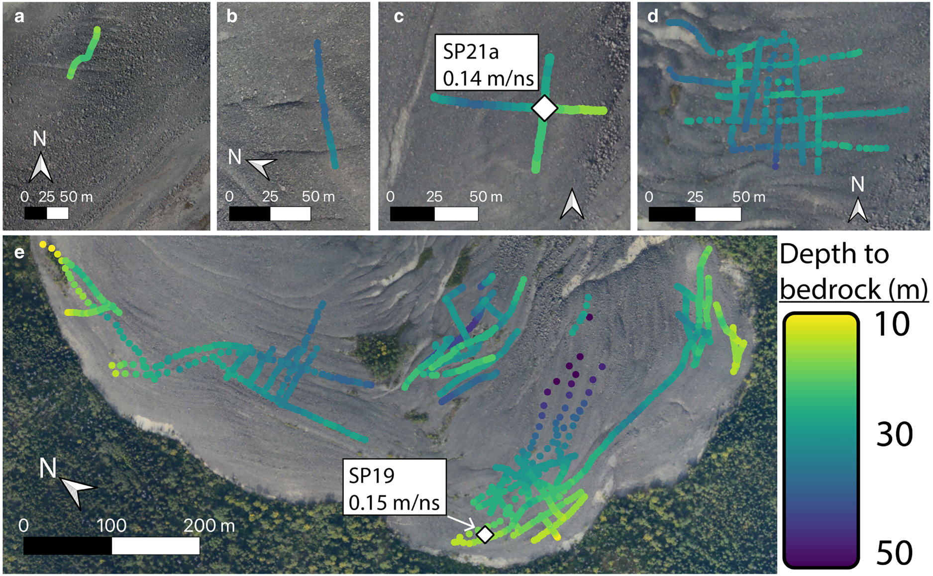
Two more CMP datasets were collected at the Sourdough site in August 2021, one of which was located at the SP19 location, with the other measurement collected at a higher elevation on the rock glaciers, labeled SP21a (Figs 7c, S5 and S6). Location SP19 returned a wave speed of 0.15 m ns−1, replicating the March 2019 measurement, while SP21a indicated a wave speed of 0.14 m ns−1. CMP measurements were not collected near the upper end of the rock glacier due to time constraints. After applying the two-phase dielectric mixing models for the permittivities of ice and rock, we find the fractional ice composition of this CMP section ranges between 69 and 81%, with the best fit at 75%. The uncertainty in the velocity measurement contributes significantly more to the uncertainty in composition than the type of dielectric mixing model used, and this is consistent for all of the rock glacier analyses described below. In Figure 6, we observe that a shallow horizon consistent with the debris/ice interface has a best fit wave speed of ~0.18 m ns−1, exceeding the 0.17 m ns−1 upper bound for pure ice, which we discuss further in Section 4.3.
3.2. Galena Creek, Wyoming
We acquired common offset and common midpoint GPR surveys along longitudinal and transverse transects of the rock glacier. The surveys were acquired in two distinct zones of the rock glacier: the mid-glacier trunk and the upper cirque. Four CMP surveys were acquired in the glacier trunk, centered on two midpoints. The first pair (Figs 8 and 9) was collected at location GC2020a and were oriented approximately perpendicular to one another in order to test the effect of the survey orientation on the measured wave speed. Both surveys initially yielded wave speeds greater than our assumed physical upper limit in ice (0.17 m ns−1) before a reflector dip correction, but the common-offset surveys show that the reflector is dipping relative to the surface in both orientations. After applying a dip correction for each orientation, both surveys return a wave speed of 0.167 m ns−1 and apparent reflector dips of ~12° and 25°.
50 MHz longitudinal transect and CMP wave speed analysis results along the trunk of Galena Creek, Wyoming at CMP location GC20a. The gold segments in (b) indicate interpreted direct and headwave arrivals in the data, labeled ‘D’ and ‘H’, respectively. The wave speed here is estimated to be 0.168 m ns−1 (d).

(a) 200 MHz transverse transect showing location of the CMP at location GC20a and perpendicular to that in Figure 8. The blue dashed line represents the interpreted reflector at the base of the ice, used for the dipping reflector analysis. The magenta dashed line shows the flat near-surface debris/ice interface. The gold segments in (b) indicate interpreted direct and headwave arrivals in the data, labeled ‘D’ and ‘H’, respectively. After correcting for dipping reflectors (d), the wave speed is estimated to be 0.167 m ns−1.

Figure 8 shows the results for the longitudinal orientation, while Figure 9 shows the results for the transverse survey at this location. This equivalent corrected wave speed for the same sample location at different CMP orientations supports the hypothesis that reflector dip influences the apparent radio wave speed using CMP surveys. This analysis suggests that the dip of the reflector should be considered when conducting a rock glacier CMP survey, especially when the dip of the reflector exceeds ~10° relative to the surface.
A second pair of CMP surveys (Figs S2 and S3) was collected at GC20b, ~15 m west of GC20a, in order to test the lateral change in rock glacier composition and geometry. One survey was collected at 50 MHz and the other was collected at 200 MHz, and they shared the same transverse orientation. Both of these surveys indicate a wave speed of 0.167 m ns−1 and a 10° subsurface dip from a reflector that has a low-offset travel time of ~250 ns. Since all four of these adjacent measurements center around the value of 0.167 m ns-1 with an uncertainty of ~0.01 m ns−1, this wave speed is assumed for all of the depth corrections of the common-offset radargrams collected at the glacier trunk. These surveys are nearest to the recovered ice core described by Clark and others (Reference Clark1996) and Steig and others (Reference Steig, Fitzpatrick, Potter and Clark1998), and this proximity is consistent with the high ice fraction at depth inferred from the wave speed. The 200 MHz survey at GC20b also resolved a near surface reflector interpreted to be the debris/ice interface corresponding to a wave speed of ~0.11 m ns−1, and these results are discussed in comparison with other debris wave speed measurements below.
In addition to the CMP experiments conducted at the mid-glacier trunk, another CMP was collected with a longitudinal profile where the slope breaks at the exit to the upper cirque (GC19; Fig. 10). The least squares fit and reflector dip correction returned a wave speed of 0.165 m ns−1 with a reflector dip of ~7°, consistent with very high ice content at this location on the glacier. We use this result of 0.165 m ns−1 as the bulk velocity for depth corrections of common offset GPR profiles collected near CMP GC19 at the cirque outlet. The locations and wave speed results for the Galena Creek CMP surveys are mapped in Figure 11, along with the corresponding bulk rock glacier thickness estimates. The rock glacier ranges in thickness from ~5 to 60 m, demonstrating the presence of a narrow but thick ice deposit in the center of the valley surrounded by remnant moraines.
50 MHz longitudinal profile at the cirque outlet of Galena Creek, Wyoming (CMP location GC19) shown with the results of the wave speed and dipping reflector analysis, indicating a wave speed of ~0.165 m ns−1.

Bulk rock glacier thickness at Galena Creek, Wyoming, estimated from 2016, 2019 and 2020 GPR survey data. The location of each map panel is shown on the left side of Figure 2. The diamonds show the locations of the CMP wave speed measurements for these thickness estimates. Map projection: WGS84/UTM 12N.

3.3. Sulphur Creek, Wyoming
Our campaign produced the first known GPR datasets at Sulphur Creek. We acquired common offset and common midpoint surveys on the upper (SC20a) and lower (SC20b) portions of the rock glacier system. After least squares analysis and comparison with diffraction hyperbolas in the common offset data, this rock glacier displays two zones with distinct radio wave speeds: the upper rock glacier has a wave speed near that of pure ice (~0.17 m ns−1, Fig. 12), while the lower rock glacier shows a significantly lower wave speed of ~0.147 m ns−1 after correcting for a 30° reflector dip (Fig. 13), indicating a dielectric constant consistent with a volumetric ice fraction of ~⅔. This decrease in ice content supports the interpretation of a transition from a debris-covered cirque glacier to an ice-cored rock glacier along the longitudinal profile of the valley (Petersen and others, Reference Petersen2019b).
100 MHz profile collected at upper Sulphur Creek, Wyoming (SC20a). The wave speed and dipping reflector results are consistent with nearly pure glacial ice. The gold segments in (b) indicate interpreted direct and headwave arrivals in the data, labeled ‘D’ and ‘H’, respectively. Here, the wave speed is interpreted as 0.17 m ns−1 (d).

50 MHz profile and wave speed analysis results at lower Sulphur Creek, Wyoming (SC20b). After dipping reflector correction, the wave speed value is ~0.147 m ns−1, consistent with that of ice-cemented rock glaciers. The gold segments in (b) indicate interpreted direct and headwave arrivals in the data, labeled ‘D’ and ‘H’, respectively. After dipping reflector correction (d), the wave speed is interpreted as 0.147 m ns−1.

Although the 1σ uncertainties of these wave speeds are both ~0.01 m ns−1, we consider 0.17 m ns−1 to be the physical upper bound for pure glacial ice and assume this value for the depth corrections of ice thickness on the upper rock glacier (Fig. 14a–c). The wave speed of 0.147 m ns−1 is assumed for depth corrections on the lower rock glacier (Fig. 14d), and the uncertainty envelope here allows for an ice fraction ranging from 62 to 84% (Table 2). After applying the two wave speed measurements to the upper and lower parts of the rock glacier, the upper ice-cored zone exhibits a thickness ranging from ~2 to 20 m of pure ice, while the lower section indicated ice-cemented debris occupying a trough almost 40 m deep.
Bulk rock glacier thickness at Sulphur Creek, Wyoming, estimated from 2019 and 2020 GPR survey data. The location of each map panel is shown on the right side of Figure 2. The diamonds show the locations of the CMP wave speed measurements for these thickness estimates. Map projection: WGS84/UTM 12N.

3.4. Gilpin Peak, Colorado
We acquired CMP data, debris thickness measurements and images of rock glacier structure at 50, 100 and 200 MHz. The 50 MHz CMP was located over complex dipping reflectors, which led to a value of 0.17 m ns−1 for the initial bulk wave speed fit when assuming a flat reflector (Fig. 15). However, previous results and the thick debris layer on the lower portion of the rock glacier suggest the wave speed should be lower than that of pure ice. Applying the travel time slope of 10 ns m−1 derived from subsurface reflectors in the common offset image can explain the unexpectedly high best fit apparent wave speed. This travel time slope corresponds to a reflector dipping ~35° below a medium of 0.14 m ns−1 (~65% ice), which is greater than the 0.12 m ns−1 wave speed interpreted from the Degenhardt and others (Reference Degenhardt, Giardino and Junck2003) survey. The difference in these wave speed measurements could have a significant effect on regional estimates of ice storage, both through calculated rock glacier volume and ice fraction, and we discuss the discrepancy between measured wave speed values below. Using the updated value of 0.14 m ns−1, we find that Gilpin Peak Rock Glacier approaches a thickness of 45 m of ice-cemented debris (Fig. 16a). The thickness of the debris ranges from 1.1 to 2.4 m (Fig. 16b) and the properties of this supraglacial debris layer are discussed in the context of all of our field sites in the following section.
50 MHz survey at Gilpin Peak, CO with interpreted horizons (blue) and CMP section location (GP19). The steep reflectors explain the unexpectedly high apparent wave speeds, and after reflector dip correction (d) the wave speed is estimated to be ~0.14 m ns−1.

Gilpin Peak, Colorado: (a) map of rock glacier thickness derived from the 25 MHz GPR travel times of Degenhardt and others (Reference Degenhardt, Giardino and Junck2003), using an updated bulk wave speed of 0.14 m ns−1. The diamond shows the location of the 2019 CMP wave speed measurement (50 MHz; see Fig. 15), which is within ~100 m of the 2003 CMP and agrees with the reprocessed results. (b) Debris thickness map using the 100 and 200 MHz 2019 GPR data assuming a debris wave speed of 0.1 m ns−1 (see Section 3.5). Map projection: WGS84/UTM 13N.

3.5. Properties of the supraglacial debris
After estimating the bulk rock glacier radio wave speed through CMP analysis and dip correction, estimating the wave speed of the supraglacial debris layer further constrains the dielectric properties of the rock glacier and provides more robust GPR measurements of debris thickness. The relatively thin debris layer (~2 m) at each of our field sites prohibits shallow CMP wave speed measurements with 50 and 100 MHz surveys because their wavelengths are comparable to the thickness of the debris which leads to the direct and refracted headwave arrivals obscuring the debris/ice reflection, especially at larger offsets. However, we collected 200 MHz CMP surveys at Galena Creek and Sourdough that both resolved a shallow reflection consistent with the low-offset travel times of the interpreted debris–ice contact.
At Sulphur Creek, the upper cirque contained relatively thin debris (<1 m), which provided an opportunity to directly observe the debris/ice contact. We acquired a 200 MHz GPR profile where a shallow reflection interpreted as the debris/ice interface is detected, so we excavated through the debris layer at this location to directly measure wave speed by dividing the measured depth by one-way travel time. Our observations at this excavation location are illustrated in Figure 17 and mapped in comparison with other manual and GPR-derived debris thickness measurements at Sulphur Creek in Figure 18. We found grain sorting within the debris at this excavation along with the pits dug in thinner debris: grain size consistently decreases with depth in the debris layer. The relative roles of water infiltration and debris motion with glacier flow in the sorting of debris clasts remain unknown, but the excavation revealed a significant amount of pore water under a pressure gradient that continuously filled the bottom of excavation. Additionally, we observed an impermeable layer of refrozen, ice-cemented debris overlying clean ice assumed to be of glacial origin, further suggesting a significant role of meltwater in the evolution of terrestrial rock glaciers. Future work may consider three-phase dielectric mixing models in order to include the contributions of liquid water or pore space.
Observations for surface debris wave speed experiment. (a) Context view of full ~1 m excavation in the debris. (b) Close-up of the debris–ice contact at the base of the excavation. Note the accumulation of water seeping from the thin saturated film at the top of the ice. (c) Stratigraphic observations of the debris layer and debris–ice contact overlying clean ice interpreted to be of glacial origin. (d) 200 MHz GPR profile and interpretation at the location of the excavation (white circle, corresponding with excavation location in Fig. 18).

Debris thickness at Sulphur Creek, Wyoming, measured directly through debris pits (⩽90 cm depth, marked as triangles) and GPR interpretation (⩾90 cm depth, marked as points). The white diamond shows the location where a manual thickness measurement was tied to a GPR reflector at 90 cm depth, resulting in the wave speed used for all rock glacier debris thickness measurements in this study (see Fig. 17). Panel locations are shown in the Sulphur Creek map in Figure 2 (note: debris thickness was not measured in panel ‘c’ in the Sulphur Creek context map, therefore panel ‘c’ in this figure corresponds with the region labeled ‘d’ on the Sulphur Creek map in Fig. 2). Map projection: WGS84/UTM 12N.

Since there is a thin transition zone of ice-cemented debris in the observed debris profile and only one discernible shallow reflection in the GPR profile, it is possible that we are detecting the return from the top of the ice-cemented debris and associated water film at 70 cm, we may be detecting the interface between the ice-cemented debris and glacial ice at 90 cm or the return could be the superposition of reflections from both interfaces since the ice-cemented layer is thinner than the GPR vertical resolution. With an interpreted 17 ns TWTT to the first break of the reflection, the 90 cm interface implies a wave speed of 0.105 m ns−1 in the debris layer (ɛ ≈ 8), while a reflection from the 70 cm interface is consistent with a wave speed of 0.08 m ns−1 (ɛ ≈ 13). Since the excavated debris section appeared to be located at a point of runoff convergence on the rock glacier and the observed water content was high, we consider that this location may have the slower wave speed and higher dielectric constant, but this is likely a lower bound for generalized debris wave speed, as other locations could have drier debris.
Our 200 MHz CMP survey at Galena Creek and the survey conducted by Petersen and others (Reference Petersen, Levy, Holt and Stuurman2019a) both indicate shallow wave speeds which are lower than that of the deeper measurements of the bulk section, with the lower bounds approaching 0.11 m ns−1. Since these shallow reflectors are not detectable at offsets much greater than their depth, the uncertainty is higher for the shallow CMP-derived wave speeds. If there is an ice-cemented debris layer separating the unconsolidated debris from the glacier ice, such as the layer observed at upper Sulphur Creek, the radar wave may be sampling this sub-wavelength scale layer at the largest detectable offsets, accounting for the slight increase in CMP debris wave speed compared to the direct measurement. For this reason, we take the mid-range value of 0.1 m ns−1 (ɛ debris = 9) for all of our debris thickness estimates at Gilpin Peak, Galena Creek, Sulphur Creek and Sourdough, assuming a homogeneous dielectric constant for the surface debris layers and englacial lithic inclusions in the bulk dielectric mixing models (Figs 16, 18–20). However, the 100 and 200 MHz CMP winter surveys at Sourdough, AK returned shallow reflections with best fit wave speeds that clearly exceeded the deeper bulk wave speed by more than 1 std dev. (Fig. 6): the shallow reflection's best fit was 0.18 m ns−1 with an uncertainty of ~0.015 m ns−1, while the bulk wave speed was measured to be 0.149 m ns−1 with an uncertainty of ~0.005 m ns−1, a factor of 3 less than the shallow uncertainty.
Debris thickness measurements at Galena Creek, Wyoming, using a constant wave speed of 0.1 m ns−1. Panel locations are shown in Galena Creek map in Figure 2. Map projection: WGS84/UTM 12N.

Depth to the debris/ice contact from 100 and 200 MHz GPR surveys on Sourdough Rock Glacier, assuming a debris layer wave speed of 0.1 m ns−1. The location of each panel is shown in Figure 1. Map projection: WGS84/UTM 7N.

The snow depth during GPR data acquisition at Sourdough was less than the lower limit for detection (~1 m) at the GPR frequencies used. Furthermore, the winter temperatures make it likely that the liquid water content of the debris at this time was negligible. Both winter and summer results at the same location on the rock glacier (SP19) indicate a bulk wave speed of ~0.15 m ns−1, with a shallow reflector interpreted to be the debris layer producing an increased wave speed measurement and higher uncertainty relative to those of the basal reflection (Figs 6 and S4). CMP measurements acquired at other locations on the rock glacier in summer 2021 show a similar pattern (Figs S5 and S6), indicating no significant seasonal influence on the wave speed measurement. The apparent increase in wave speed for the Sourdough debris layer may be caused, in part, by the shallow depth of the debris/ice interface relative to the antenna offset needed to measure the change in travel time, leading to imprecise wave speed measurements. Wave speed inflation may also arise from small-scale variations in debris thickness, leading to sloped interfaces with respect to the CMP orientation.
Additionally, the increased debris layer wave speed measurements at Sourdough may also be an artifact from the shallow reflector interacting with a refracted headwave arrival. Assuming this near-surface arrival is a headwave, which is linear in travel time vs offset and is generated when an underlying medium has a faster wave speed than the overburden layer, the underlying layer's wave speed is ~0.144 m ns−1 (Telford and others, Reference Telford, Geldart and Sheriff1990). This value is consistent with the bulk rock glacier measurement and the observation of a headwave implies a supraglacial debris layer with a slower wave speed. Due to these ambiguous features in the shallow CMP data, we take all debris layer wave speeds to be 0.1 m ns−1, directly measured by tying the debris excavation thickness with GPR travel time at Sulphur Creek, Wyoming (Fig. 17). This wave speed corresponds to a dielectric constant of 9. We note that the heterogeneity of dielectric properties in the debris layer remains a primary source of uncertainty in GPR estimations of local debris layer wave speed, thickness and bulk ice fraction. Surveys on Ngozumpa Glacier, Nepal, measured debris wave speeds exceeding 0.15 m ns−1 using a depth/travel time tie (Nicholson and others, Reference Nicholson, McCarthy, Pritchard and Willis2018). CMP measurements of the debris wave speed on Lirung Glacier, Nepal, ranged from 0.106 to 0.129 m ns−1, with the lowest values appearing to correlate with the flattest reflectors (McCarthy and others, Reference McCarthy, Pritchard, Willis and King2017). For simplicity, we assume a constant value of 0.1 m ns−1 for the debris layer at all of our study sites based on our excavation/GPR tie point at upper Sulphur Creek. Further characterization of the variability of dielectric properties of supraglacial debris could help refine these estimations.
Our assumption of 0.1 m ns−1 for the debris wave speed produces GPR-derived thickness measurements which reveal trends among our study sites. In general, the debris thickness is greater for the ice-cemented zones and lower portions of the rock glaciers (>2 m for Sourdough, Gilpin Peak and lower Sulphur Creek, where the maximum ice fraction is <75%) than the ice-cored regions (0.2–1 m for Galena Creek and upper Sulphur Creek, where ice fraction is >0.8). Additionally, both the ice-cemented and ice-cored zones show undulations in debris thickness correlating with the spatial scale of the furrow and ridge morphology (Figs 16, 18–20). This is consistent with observations of compressive buckle folding in the debris layer (Frehner and others, Reference Frehner, Ling and Gärtner-Roer2015). Some very thick debris measurements may be related to the intersection of internal debris layers with the surface, such as upper Galena Creek (Fig. 19a). These thickness variability observations will constrain thermal effects of the debris layer on the subsurface ice while informing models of debris layer processes and their relationships with rock glacier dynamics and internal structure.
4. Discussion
4.1. Comparison with previous Gilpin Peak results
In addition to the data we collected at our field sites from 2018 to 2021, we used our least squares analysis method to process a digital interpretation of a 25 MHz CMP survey acquired in a previous study at Gilpin Peak, Colorado (Degenhardt and others, Reference Degenhardt, Giardino and Junck2003; labeled D+03 in Fig. 21). We find that the bulk wave speed above a near-surface reflector where t 0 = 127 ns agrees with the 2003 interpreted wave speed of 0.12 m ns−1 with a detectable signal up to ~15 m offset. In the 2003 automated wave speed analysis, the shallow high-likelihood region is centered at ~0.12 m ns−1 down to 100 ns. We suggest that this value corresponds to our shallow 0.12 m ns−1 result, and this region is the source of the interpretation for best-fit bulk wave speed presented by Degenhardt and others (Reference Degenhardt, Giardino and Junck2003). However, deeper hyperbolas are evident in the D+03 data; we picked three additional horizons with t 0 values of 176, 300 and 364 ns in the 25 MHz plot. All of these horizons fit wave speeds of 0.14 m ns−1 with uncertainties of ⩽0.01 m ns−1. Since each CMP horizon contains information about the wave speed of the overlying bulk material, the average wave speed of the sounding column will be associated with the deepest reflector, not the strongest. The 0.14 m ns−1 result is consistent with a weaker but consistent band of increased likelihood in the D+03 wave speed plot ranging from ~150 to 400 ns (Fig. 21c) that was ignored in the original interpretation of bulk wave speed; the width of this 0.14 m ns−1 band is also comparable with the derived uncertainty value near 0.01 m ns−1. The deeper reflectors may appear to have lower amplitudes in the automated analysis due to the algorithm's reliance on iterative stacking and constructive interference. We postulate that the automated method amplifies the stronger shallow reflections disproportionally to the relatively attenuated reflections at depth, and this bias toward a shallow signal led to the interpretation of a bulk wave speed of 0.12 m ns−1 in the previous study.
Re-analysis of 25 MHz survey collected by Degenhardt and others showing that the bulk radio wave speed through the rock glacier has a best fit of ~0.14 m ns−1. (a) Rock glacier thickness and basal elevation depth corrected from Degenhardt and others (Reference Degenhardt, Giardino and Junck2003), using wave speeds of 0.12, 0.13 and 0.14 m ns−1. (b) 2003 CMP data (Degenhardt and other, Reference Degenhardt, Giardino and Junck2003) annotated with our manual interpretations as blue dashed lines. (c) Semblance plot, modified from Figure 4a of Degenhardt and others (Reference Degenhardt, Giardino and Junck2003) to depict the digital interpretations in the CMP section and the interpreted wave speed values in the semblance plot. Degenhardt and others (Reference Degenhardt, Giardino and Junck2003) noted the 0.12 m ns−1 signal in their analysis, but neglected the deeper, less obvious signal centered ~0.14 m ns−1 that is more representative of the bulk interior of the rock glacier. (d) Best fit hyperbola for each interpreted horizon. (e) Best fit wave speeds with their uncertainties, showing a trend with depth that is similar to that observed in the semblance plot in (b).

We argue that our manual interpretation and fitting method, which considers wave speed solely as a function of CMP geometry with no dependence on received power, provides a more robust wave speed upper bound of 0.14 m ns−1 rather than the previously reported 0.12 m ns−1. The 0.14 m ns−1 wave speed is also consistent with the dip-corrected results of our GP19 survey analysis. The 2003 common offset radargram indicated nearly horizontal reflectors close to the 2003 CMP location (Degenhardt and others, Reference Degenhardt, Giardino and Junck2003), so we assume that there was negligible error due to the representation of dipping reflectors in their data. A ~15% increase in estimated bulk wave speed may seem relatively insignificant, but it leads to an increase of up to ~7 m in bulk rock glacier thickness from the interpreted 2003 data (Fig. 21a). However, if we assume relative dielectric permittivities of 3 for pure ice and 9 for lithics, this 0.02 m ns−1 increase in wave speed corresponds to an increase in local ice volume fraction from ~30 to ~60% in the two-phase mixing models (see Section 4.2). These results could significantly impact estimates of integrated rock glacier ice storage in the San Juan Mountains, and it demonstrates the sensitivity of rock glacier ice fraction estimations to the accuracy of the wave speed measurement. In consideration of the sensitivity of dielectric constant on bulk wave speed, we will discuss why an accurate and precise wave speed measurement is essential for estimating ice fraction.
4.2. Wave speed and composition
Our analyses for all sites returned GPR wave speeds consistent with ice fractions >50%, when assuming a dielectric constant of 3 for ice and 9 for rock (Table 2 and Fig. S7). The two Wyoming sites displayed evidence of clean, glacially derived ice units buried by debris on the upper portions of each rock glacier, with generally decreasing ice content toward the glacier toe. The dielectric constant of the debris inclusions is a source of uncertainty for these estimates: lower permittivities for lithics would lead to lower volumetric ice fractions for a given bulk wave speed, so these estimates should be considered an upper bound on ice content. Other uncertainty sources in our wave speed estimates include errors associated with manual interpretation and assumptions of geometric simplicity (smooth, continuous and linear interfaces relative to radar wavelength). Investigation into the effects of rough or nonhomogeneous reflectors could further account for wave speed uncertainties.
An important result of our analysis is the demonstration that dipping subsurface reflectors may lead to overestimates of bulk wave speeds with the CMP method, which has consequences for depth corrections and compositional models. Since the wave speed in rock glaciers is very sensitive to volumetric ice fraction, and several rock glacier surveys have revealed the presence of subsurface dipping reflectors, we argue that it is essential to consider the dip angle of the reflector when estimating the wave speed, especially when the dip exceeds ~10° relative to the surface. Above this 10° threshold, the deviation from the true wave speed begins to exceed the uncertainty in the measurements, so we suggest that all future rock glacier surveys correct for reflector dip when using CMP wave speed analysis. Indeed, any geologic target with dipping subsurface structures should use the techniques employed in this paper for accurate CMP wave speed analysis. Dipping reflectors influenced the apparent wave speed at Galena Creek, Sulphur Creek and Gilpin Peak. Accounting for dipping reflectors ensures that wave speeds remain physically possible (not exceeding 0.17 m ns−1, such as measurements at upper Galena and Sulphur Creek), and it can also help to prevent overestimates in ice content where the rock glacier contains less ice (e.g. Gilpin Peak and lower Sulphur Creek).
The CMP survey at Sourdough, Alaska had no steeply dipping reflectors influencing the wave speed measurement and returned a value of 0.149 m ns−1 for each frequency at this location. This wave speed is consistent with an ice fraction of ~75%, but it does not conclusively delineate whether the ice is glacigenic or periglacial in origin. Since this value is on the lower end of our wave speed results and no exposures of high-purity glacial ice were observed at this location, it may lend support to the periglacial interpretation. However, this measurement was acquired near the lowest elevation on the rock glacier where the bulk glacier thickness is relatively low and the debris layer is relatively thick, so it is possible that ice fraction increases with increasing elevation at Sourdough. Additional CMP measurements toward the head of the rock glacier would help elucidate this possibility. In general, our results of >50% bulk ice fraction, debris layer thicknesses of a few meters and a maximum rock glacier thickness >50 m are comparable with previous observations at nearby Fireweed Rock Glacier, which is ~20 km away (Elconin and LaChapelle, Reference Elconin and LaChapelle1997; Bucki and others, Reference Bucki, Echelmeyer and MacInnes2004). Additional GPR surveys at Sourdough could reveal spatial trends in ice fraction along the profile of the rock glacier while improving the thickness measurements mapped in Figure 7, which would provide more information about the relationship between its internal structure and formation processes.
At Galena Creek, Wyoming, one question arises from the results: what causes the slight increase in measured bulk wave speed and ice fractions at CMP locations moving down-glacier from the cirque to the trunk? This is counterintuitive when considering the tendency of ice accumulation to increase with elevation. Perhaps the highest surveys near the cirque head, which measured an average wave speed of ~0.16 m ns−1 (Fig. S8) and detected several closely spaced internal reflectors (Petersen and others, Reference Petersen, Levy, Holt and Stuurman2019a; labeled GC16 in Fig. 11), sampled a location with a higher debris content due to its proximity to the headwall/glacier margin and the resulting process of debris-facilitated ice accumulation. The lower surveys may have been conducted over a thicker portion of the preserved glacial ice unit, leading to a higher bulk ice content and a measured wave speed of ~0.168 m ns−1. However, the magnitudes of the uncertainties of these measurements still allow for this disparity to be smaller than the best fit values suggest, and it is likely that there is significant compositional heterogeneity within each rock glacier.
Other observations of the GPR data from Galena and Sulphur Creek support a high-purity ice core of glacial origin buried beneath the supraglacial debris at higher elevations for both sites. First, several diffraction hyperbolas are observed in the common offset profiles. These hyperbolas fit to wave speeds ranging from ~0.1 to 0.17 m ns−1 and often appear asymmetric, which is consistent with the presence of pure ice and small-scale compositional heterogeneity in the rock glaciers. The few dielectric constant measurements exceeding 10 may correspond to zones of meltwater-saturated debris near the surface. There appears to be a general trend of decreasing diffraction wave speeds (thus increasing dielectric constant, Fig. S9) moving down-glacier for both Galena and Sulphur Creek, further supporting the hypothesis of a high bulk ice fraction in their upper cirques which transitions to lower ice concentrations at lower elevations.
In addition to diffraction hyperbolas in the common offset sections, there is a distinct headwave arrival in the CMP data for some common midpoints on both Galena and Sulphur Creek (labeled ‘H’ in Figs 8, 9, 12 and 13; example data in Fig. S10). This is interpreted as the arrival that is generated from the refraction of the radio wave as it transmits from the lower-velocity debris to the higher-velocity ice-rich medium. Since this wavefront is linear in time and offset, the slope of the headwave arrival is the reciprocal of the wave speed of the higher-velocity medium (Telford and others, Reference Telford, Geldart and Sheriff1990). The headwaves observed in our data fit wave speeds of ~0.17 m ns−1, further supporting the existence of a nearly pure ice core buried beneath the debris at these locations. Uncertainty analyses were not performed for the common offset hyperbolas or CMP headwave arrivals, but their overall trends support the results of the CMP wave speed analysis, indicating a high-elevation ice core and a decrease in ice content moving down glacier at Galena and Sulphur Creek, Wyoming. This may signify a transition from an ice core of glacial origin to a periglacial ice-cemented rock glacier with decreasing elevation at both of these sites. The correlation of the GPR wave speeds, surficial ice exposure observations and borehole data (Clark and others, Reference Clark1996; Potter and others, Reference Potter1998; Steig and others, Reference Steig, Fitzpatrick, Potter and Clark1998) at Galena and Sulphur Creek support the interpretation that rock glaciers with a dip-corrected wave speed between 0.16 and 0.17 m ns−1 likely have a high-purity ice core of glacial origin.
This study and many previous authors have demonstrated the heterogeneity in GPR reflector geometry and wave speed structure of rock glaciers around the Earth (Table 1). When dipping reflectors are present, a significant challenge in accounting for apparent wave speed inflation is the uncertainty in the orientation of the CMP survey in relation to the common-offset profile, since the error in wave speed is related to the apparent dip of the subsurface reflector observed from the CMP orientation with respect to the true strike and dip of the reflector. Relatively few of the publications referenced in Table 1 provide survey orientations, data, analysis details or assumptions for their wave speed estimates.
Our experiment examining the effects of dipping reflectors on estimated wave speed shows the importance in accounting for internal structure and reflector geometry in rock glacier GPR wave speed estimations. Otherwise, it could result in inaccuracies propagated to assessments of individual rock glacier geometry and sums of local to global ice volumes preserved beneath debris. For example, Jones and others (Reference Jones, Harrison, Anderson and Betts2018a) estimated an ice mass of 83.72 ± 16.74 Gt stored in the global rock glacier population using an assumed range of 40–60% volumetric ice fraction, but this global ice mass could be greater if a significant percentage of rock glaciers contain glacial ice cores with bulk ice fractions much >60%. Precise compositional measurements over a range of sites could further reduce the uncertainty of the global estimate, while also elucidating the relative importance of rock glaciers, debris-covered glaciers and bare ice glaciers in different hydrological systems (e.g. Himalayan vs Andean glacier populations; Jones and others, Reference Jones2018b).
We reiterate that our assumption of a dielectric constant of 9 for the lithic inclusions remains a primary source of uncertainty in calculating the ice fraction with dielectric mixing models using bulk wave speed. Better characterization of the intra- and inter-site variability in the dielectric properties of the debris could further refine estimates of both debris thickness and bulk ice fraction. More work is needed to understand the effects of local lithology and mineralogy on the dielectric properties and thermal insulation of the debris layer and the broader effects on rock glacier dynamics. For future surveys measuring radio wave speed on rock glaciers using the CMP method, we recommend a standard method of collecting common-offset transects to associate with each CMP orientation and assess the reflector geometry for the wave speed estimate. This replicable method will improve the precision of compositional and geometric measurements for rock glaciers, and these measurements can be applied to dynamic viscoelastic flow models for comparison with photogrammetrically derived surface displacements to better understand rock glacier formation and evolution.
5. Conclusion
When using GPR in a common midpoint configuration to measure the structure and composition of any geophysical target with subsurface reflectors dipping ~10° relative to the surface, it is important to collect co-located and coeval common offset profiles to determine the influence of reflector geometry on estimated wave speed. This is especially true if the target deforms over the course of a multi-year field campaign where it may be impractical or impossible to replicate the position and acquisition parameters of a previous year's measurement. Increased reflector dip and complexity generally increases the uncertainty of the measurements, so future surveys that target continuous, flat reflectors while considering the small-scale compositional heterogeneity throughout each site may best characterize the dielectric properties of rock glaciers and their overlying debris. The accuracy and precision of wave speed measurements directly impact compositional estimates through dielectric mixing models while also affecting depth corrections of GPR travel time data. We have shown an example of this procedure used to characterize rock glacier composition and geometry. These compositional estimates of individual rock glaciers will have a significant impact when extrapolated to total ice volume of regional or global rock glacier populations, which subsequently affects our understanding of alpine hydrological systems.
We used our method of geometrically corrected wave speed measurement to estimate the bulk composition on four rock glaciers over a range of latitudes, elevations and geographic settings. Our results included the detection of nearly pure ice cores at upper Galena and Sulphur Creek, Wyoming, consistent with previous results at Galena Creek (Potter and others, Reference Potter1998; Petersen and others, Reference Petersen, Levy, Holt and Stuurman2019a). We also measured lower volumetric ice fractions of ~60–70% at Gilpin Peak, Colorado, and Sourdough, Alaska. These compositional results may be affected by the uncertainty in the dielectric permittivity of the lithic inclusions within each rock glacier, but our analysis shows that the ice fraction at the Gilpin Peak site could be twice as much as previous estimates of 30%. Understanding the compositional trends of ice-cored and ice-cemented rock glaciers will help the cryospheric community decipher the formation mechanisms and ice origins at different sites, which will further improve our generalized models for rock glacier evolution.
We also examined the wave speed within the surface debris layer. Our best determination for the dielectric constant of the debris layer is ~9, although these shallow measurements have a relatively high uncertainty throughout all of the field sites. Further constraints on the dielectric properties of the debris will improve estimates of bulk rock glacier composition through dielectric mixing models. Our measured bulk and debris layer wave speeds were used to convert GPR travel time measurements into depth to bedrock and debris layer thickness estimates. These compositional and geometric observations will inform future models of rock glacier flow and ice/rock dynamics in terrestrial and planetary settings.
Supplementary material
The supplementary material for this article can be found at https://doi.org/10.1017/jog.2022.90
Data
All data and associated Supplementary materials reported in this paper are openly available online at https://doi.org/10.25422/azu.data.19495178.
Acknowledgements
This study was funded by NASA Solar System Workings grant 80NSSC19K0561. We thank Michael Christoffersen, Brandon Tober, Stefano Nerozzi, Tyler Kuehn, Victor Devaux-Chupin, Cassie Stuurman, Ben Cardenas and Joe Levy for their assistance and advice with field data acquisition. We thank two anonymous reviewers for their constructive comments that improved the manuscript. Additionally, Eric Yould and Kurt Smith provided essential logistical support for rock glacier access in Alaska. Chris Larsen acquired the aerial imagery for the Sourdough base map, Chris Boyer acquired the aerial imagery for the Galena Creek and Sulphur Creek base maps and the Gilpin Peak base map was downloaded from the public USGS aerial imagery database.
Author contributions
TM collected the GPR data, developed the CMP analysis code, performed the wave speed/dipping reflector analysis, calculated the composition of each rock glacier and wrote the manuscript. EP collected the GPR data, performed the diffraction hyperbola analysis, provided interpretations for the results and contributed to the revision of the manuscript. JH acquired funding, provided logistical support for data collection, supervised the data analysis and contributed to the revision of the manuscript.


 Open access