


15.1 Introduction
Our use of language in daily life is rich and complex. Speaking involves the whole body, is embedded in context, and nearly always involves multiple people. Of relevance to the topic of this book, spontaneous spoken language is produced and comprehended on the fly, unfolding continuously over time. These factors contribute to the ongoing emergence of linguistic structure, which is constantly developing to meet our communicational needs. This usage-based approach to the study of language has contributed greatly to the understanding of the cognitive organization of language (Bybee, Reference Bybee, Díaz-Campos and Balasch2023; Bybee and Beckner, Reference Bybee, Beckner, Heine and Narrog2010; Christiansen and Chater, Reference Christiansen and Chater2008; Ellis, Reference Ellis2019; Hopper, Reference Hopper1987; Mithun, Reference Mithun, Givón and Shibatani2009; Mushin and Doehler, Reference Mushin and Doehler2021; Tomasello, Reference Tomasello1998, Reference Tomasello2003). The neural mechanisms supporting the use of language are likely also influenced by these processes (Scott, Reference Scott2019). However, the neural mechanisms of language are often – and perhaps usually – studied by relying on language that is abstracted away from these complexities. In this chapter, we adopt the usage-based perspective and consider the temporal unfolding of spontaneous spoken language and concurrent brain activity. We focus on the prosodic organization of speech into sequences of intonation units (Chafe, Reference Chafe1994; henceforth, IUs), and the ~1 Hz rhythms that they form (Inbar et al., Reference Inbar, Grossman and Landau2020, Reference Inbar, Genzer, Perry, Grossman and Landau2023; Stehwien and Meyer, Reference Stehwien and Meyer2022). Speech prosody is the domain of language that has to do with how pitch, duration, loudness, and other voice qualities unfold over time. Speech prosody plays a central role in communication, and – among its many functions – is used for chunking continuous speech into sequences of prosodic phrases, IUs. Cross-linguistic research suggests that IUs are fundamental to human language and constitute a universal property of language (Chafe, Reference Chafe1994; Himmelmann, Reference Himmelmann2022; Himmelmann et al., Reference Himmelmann, Sandler, Strunk and Unterladstetter2018). In the following, we survey the linguistic literature on IUs, including their formal definition and functional roles in speech (Sections 15.2 and 15.3, respectively). We continue by discussing neuroscientific findings pertaining to IUs, and their relation to low-frequency brain rhythms (Section 15.4). In addition, we review algorithmic tools for IU identification, to facilitate further investigations of IUs and the neural processes associated with them (Box 15.1). We build mainly upon Wallace Chafe’s conception of IUs, yet consider the influence of similar conceptions of prosodic chunking in a variety of research traditions. We aim to provide a comprehensive survey of current research on IUs, and to introduce them within the context of rhythms of speech, language, and the brain.
15.2 Intonation Units: Form
15.2.1 Phonetic-Prosodic Definition of IUs
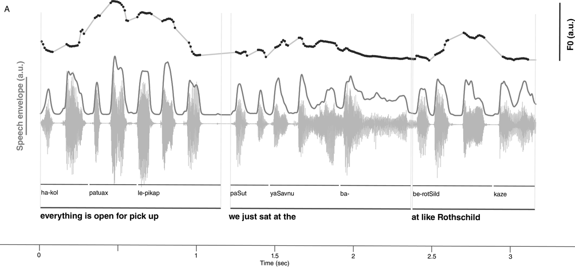
IUs are defined by a set of phonetic-prosodic characteristics whose identification is an auditory, perceptual matter (Chafe, Reference Chafe1994; Couper-Kuhlen, Reference Couper-Kuhlen1993; Couper-Kuhlen and Barth-Weingarten, Reference Couper-Kuhlen and Barth-Weingarten2011; Cruttenden, Reference Cruttenden1997; Du Bois et al., Reference Du Bois, Cumming, Schuetze-Coburn, Paolino, Du Bois, Cumming, Schuetze-Coburn and Paolino1992; Halliday, Reference Halliday1967; Kibrik, Reference Kibrik2019; Schuetze-Coburn et al., Reference Schuetze-Coburn, Shapley and Weber1991; Shattuck-Hufnagel and Turk, Reference Shattuck-Hufnagel and Turk1996). To identify IUs, one must listen to changes in pitch, duration, and loudness in the unfolding speech. Beginning with pitch, an IU is “a stretch of speech uttered under a single coherent intonation contour” (Du Bois et al., Reference Du Bois, Cumming, Schuetze-Coburn, Paolino, Du Bois, Cumming, Schuetze-Coburn and Paolino1992). Intonation refers to the modulations of pitch in speech, which are controlled by variation in the frequency of vocal fold vibrations. A coherent intonation contour is composed of a unified pitch movement, on the one hand, and a sharp change in pitch level relative to the preceding utterance, on the other. The shape of the pitch movement is often characterized by reference to its nucleus and final part, and it is critical for determining the meaning of an utterance. Fundamental frequency (F0) is the correlate of pitch in the acoustic domain. Although it is an imperfect correlate, it allows to visualize pitch movements and resets. Figure 15.1A presents the F0 time course of an example speech excerpt in which three IUs were identified.
IUs: an example sequence and duration histograms.
An example sequence of three IUs from a Hebrew phone call. From bottom to top: a literal translation of each unit; an X-SAMPA phonemic transcription of Hebrew orthographic words; the audio waveform; the speech envelope; the F0 time series. The highlighted portions in the F0 time series signify actual values measured from voiced segments. Thin lines in between provide an estimation via linear interpolation for voiceless segments and pauses. Speech recording available in Marmorstein et al. (Reference Marmorstein and Matalon2022).
Probability distribution of IU durations in six languages, calculated in 50 ms bins and pooled across multiple speakers. Overlaid are the medians (dashed line, dark gray) and the bootstrapped 95% confidence intervals of the medians (light gray).

Moving to durational characteristics, sequences of IUs include an acceleration–deceleration dynamic of syllable delivery rate. Unit-initial syllables are short and often contracted (a phenomenon termed anacrusis; Cruttenden, Reference Cruttenden1997), while utterance-final syllables are lengthened. Final lengthening is a widespread process in the languages of the world (for recent quantitative demonstrations, see Paschen et al., Reference Paschen, Fuchs and Seifart2022; Seifart et al., Reference Seifart, Strunk and Danielsen2021), and is also considered a highly reliable cue for identifying IU boundaries. The audio waveform and annotations in Figure 15.1A illustrate changes in syllable delivery rate in the example speech excerpt. However, it should be mentioned that the perception of duration is a subjective phenomenon that cannot be fully captured in timing measurements.
In terms of loudness, sequences of IUs tend to include an increase–decrease dynamic in loudness. This dynamic relies on articulatory factors. The degree of contact between articulators is strongest at the onset of a new utterance (Keating et al., Reference Keating, Cho, Fougeron, Hsu, Local, Ogden and Temple2003), and this generates resets in loudness at IU onsets. Additionally, because of the gradual decrease in articulation pressure throughout the IU and the compression of the vocal folds, the vibration of the vocal folds might become irregular and particularly slow near the end of the IU, resulting in a low, raspy voice known as creaky voice (Chafe, Reference Chafe1994).
Pauses in speech often accompany the previously mentioned characteristics. However, they are neither a necessary nor a sufficient characteristic of an IU boundary. IUs may succeed each other without any audible pause in between, and on the other hand, pauses may appear midway through an IU, without a reset in pitch level or a change in syllable delivery rate.
A single IU typically features one accented syllable. Another common configuration is two accented syllables, one primary and the other secondary. Accented syllables are prominent in comparison to surrounding ones due to the pitch movement being centered on the syllable, and they are often louder and/or longer in duration. The accent is usually placed on a lexically stressed syllable, though this is not obligatory. An example exception is the case of contrastive accenting, as in: “I said fifTY not fifTEEN” (Couper-Kuhlen and Barth-Weingarten, Reference Couper-Kuhlen and Barth-Weingarten2011).Footnote 1 See Chapter 35 and Section 6 in general for a complementary view on the rhythm of stressed syllables in speech and its importance in language acquisition.
The phonetic-prosodic definition of IUs provided so far relies on perceptual phenomena, and thus attuned listeners can identify IUs even in unfamiliar languages (Himmelmann et al., Reference Himmelmann, Sandler, Strunk and Unterladstetter2018). The characteristics may be conventionalized and acquire meaning and become language-specific phonological categories. Trivial examples may be found in the association of a specific function with a certain configuration of the coherent pitch contour. For example, it is very common for languages to use particular prosodic contours for questioning. There may be more subtle conventionalized prosodic patterns, for example for strengthening one’s own stance in interaction (Matalon, Reference Matalon, Mauri, Fiorentini and Goria2021).
Linguists have developed different systems for transcribing prosodic phenomena, reflecting a range of research traditions. Three widespread systems in current linguistic research are ToBI (Beckman et al., Reference Beckman, Hirschberg, Shattuck-Hufnagel and Jun2005; Pitrelli et al., Reference Pitrelli, Beckman and Hirschberg1994), GAT (Couper-Kuhlen and Barth-Weingarten, Reference Couper-Kuhlen and Barth-Weingarten2011; Selting et al., Reference Selting, Auer and Barden1998), and DT (Du Bois et al., Reference Du Bois, Cumming, Schuetze-Coburn, Paolino, Du Bois, Cumming, Schuetze-Coburn and Paolino1992), and they all converge on the phonetic-prosodic chunking of speech just described. ToBI (Tones and Break Indices) grew out of the autosegmental-metrical approach to the study of intonation (Ladd, Reference Ladd2008; Pierrehumbert, Reference Pierrehumbert1980). GAT (Gesprächsanalytisches Transkriptionssystem, from German: discourse and conversation-analytic transcription system) was developed as an extension of the transcription style used in conversation analysis (Jefferson, Reference Jefferson and Lerner2004) for the representation of prosody. Similar to GAT, DT (Discourse Transcription) also emerged from the study of everyday conversation. These three systems developed in different research traditions for distinct uses and under varying sets of assumptions. However, they all include explicit marking of IUs, though they call them by different names: intonation units is the term used in DT, GAT uses the term intonation phrases, and ToBI (intermediate) intonational phrases. In the context of transcribing speech, it should be noted that IU boundary annotations tend to be relatively robust between transcribers (e.g., Himmelmann et al., Reference Himmelmann, Sandler, Strunk and Unterladstetter2018; Kibrik, Reference Kibrik2019; Pitrelli et al., Reference Pitrelli, Beckman and Hirschberg1994).
When speech is segmented into IUs, the resulting segmentation reflects an assumption that prosodic phrase boundaries are binary in nature. As speech unfolds, a prosodic boundary either occurs or does not. This assumption may be too simplistic a conception of how speakers actually structure their speech prosodically (Barth-Weingarten, Reference Barth-Weingarten2016; Barth-Weingarten and Ogden, Reference Barth-Weingarten and Ogden2021). Specifically, one can question the utility of a single prosodic cue versus several. Research on talk-in-interaction suggests that granularity may serve a function. For example, the prosodic boundaries between episodes in a narrative (Chafe, Reference Chafe1980) or frames in conversation (Goffmann, Reference Goffman1981) come in different strengths, depending on the amount of reorientation required to process the change.
15.2.2 Temporal Structure of IUs
Previous studies characterized the length of IUs using different measurement styles. One method measures the number of words per IU (Chafe, Reference Chafe1994; Himmelmann et al., Reference Himmelmann, Sandler, Strunk and Unterladstetter2018; Pawley and Syder, Reference Pawley, Syder and Riggenbach2000). We present the counts aggregated from these studies in Table 15.1. However, as we have demonstrated elsewhere (see Box 2 in Inbar et al., Reference Inbar, Grossman and Landau2020), what constitutes a word varies greatly across languages (Haspelmath, Reference Haspelmath2011), and so it is difficult to infer the temporal structure of IUs from word counts. Other studies measured the number of syllables per IU (see Table 15.1). Syllable structure also varies across languages, yet unlike the case for words, it is possible to find a common formal characterization for them: Syllables evolve around a vocalic nucleus (e.g., Blevins, Reference Blevins2006). Thus, it is possible to count and measure the durations of syllables in a cross-linguistically sensible way (Greenberg, Reference Greenberg2022; Greenberg et al., Reference Greenberg, Carvey, Hitchcock and Chang2003) and obtain an indirect estimation of IU length. Recent studies found that languages consistently differ in syllable production rate (Coupé et al., Reference Coupé, Oh, Dediu and Pellegrino2019; Pellegrino et al., Reference Pellegrino, Coupé and Marisco2011). Currently, it is unclear if this difference leads to differences in IU rates across languages, or if languages differ in the syllable counts per IU. Finally, it should be noted that an estimation of IU length does not capture information about the temporal structure of IU sequences.
| Language | Word count | Syllable count | IU type (see Section 15.3) | Reference |
|---|---|---|---|---|
| English | 4.84 | Substantive, e.g., “we had such a nice day” | Chafe (Reference Chafe1994) | |
| 1.36 | Regulatory, e.g., “and” “well” “umm” | |||
| Seneca (Iroquoian, east USA and Canada) | 2 | Any | ||
| German | 5.20 | Any | Himmelmann et al. (Reference Himmelmann, Sandler, Strunk and Unterladstetter2018) | |
| Papuan Malay | 4.08 | Any | ||
| Wooi (Austronesian, West Papua) | 3.63 | Any | ||
| Yali (Papuan highland, West Papua) | 3.37 | Any | ||
| Modern Hebrew | 2.18 | Any | Inbar et al. (Reference Inbar, Genzer, Perry, Grossman and Landau2023) | |
| English | 7–10 | Excluding IUs “consisting of a connective or an exclamation (e.g., Alors, ‘Therefore’, in French)” | Jun, Reference Jun and Jun2005 | |
| French | 7–10 | |||
| Japanese | 7–10 | |||
| Korean | 12–15 |
In a recent study, we provided a quantitative characterization of the temporal structure of IU sequences (Figure 15.1B; see also Figure 2 in Inbar et al., Reference Inbar, Grossman and Landau2020). We analyzed audio recordings of spontaneous speech in six languages from different families and from different parts of the world. We used IUs as times of interest for analyzing periodicities in the speech envelope. The speech envelope (see Figure 15.1A) is a representation of amplitude fluctuations in speech, and it therefore presumably captures two of the cues for IU boundaries: (1) resets in loudness, and (2) the acceleration–deceleration dynamic of syllable delivery, because one of the sources for the amplitude peaks measured in the speech envelope is the succession of syllable nuclei (see Section 2 for further discussion of amplitude fluctuations in speech). We found that ~1 Hz fluctuations in the speech envelope aligned consistently with IU onset times, and consequently delineated the rate of the unfolding of IUs at a rate of approximately one per second. This finding held in each of the six languages that we studied, despite substantial differences between them in grammatical, areal, genealogical, and socio-cultural parameters. Stehwien and Meyer (Reference Stehwien and Meyer2022) replicated these results in an additional language, finding that sequences of 2–5 IUs in German are periodic at 0.8–1.6 Hz. This study used a different statistical framework and radio news broadcasts rather than recordings of spontaneous speech, providing further validity and robustness to the finding. Together, these studies (Inbar et al., Reference Inbar, Grossman and Landau2020; Stehwien and Meyer, Reference Stehwien and Meyer2022) corroborate early reports on the temporal structure of IU sequences of spoken American English (Chafe, Reference Chafe and Tomlin1987; Couper-Kuhlen, Reference Couper-Kuhlen1993) with quantitative evidence from a variety of languages.
This subsection described the temporal structure of sequences of IUs, namely, that one IU succeeds another at the rate of approximately one IU per second. Although the rhythm we characterize is not an isochronous beat, to which one can dance, tap, or nod (Cummins, Reference Cummins2009), nuanced research can demonstrate cases where the approximate rhythmic structure does, in fact, shape behavior. To conclude this subsection, we would like to present evidence that in local contexts, sequences of IUs, or rather sequences of accentuated syllables within IUs, do happen to give rise to rhythmicity in the sense of affording synchronization. Linguists have studied such rhythmic structures in talk-in-interaction (Auer et al., Reference Auer, Couper-Kuhlen and Müller1999; Couper-Kuhlen, Reference Couper-Kuhlen1993; Marmorstein and Matalon, Reference Marmorstein and Matalon2022). In their analyses of stretches of spontaneous spoken language, they identify rhythmic structures that are composed of at least three accentuated syllables (e.g., in three IUs) that are evenly spaced in time. It is possible to tap along to these structures, and there is further evidence that interlocutors perceive this rhythmicity and act on it during interaction. Specifically, when interlocutors take turns at talk, rhythmic structure can be constructed also across their turns, giving rise to rhythmic integration (Auer et al., Reference Auer, Couper-Kuhlen and Müller1999). When one interlocutor integrates their speech into a rhythm set by another at a point of speaker change, this promotes intact interactional exchange. However, when the speech is rhythmically off, interlocutors “engage in supplementary inferencing to account for the departure from expectation” (Auer et al., Reference Auer, Couper-Kuhlen and Müller1999, p. 70). In other words, the talk following a potential point of integration across turns provides evidence for the rhythmicity. The phenomenon of rhythmic integration highlights the importance of studying spontaneous speech in interactional contexts, for finding rhythm in language.
The identification of IUs has been for a long time an auditory, perceptual matter. The task of manual speech segmentation is laborious and time-consuming, and cannot keep up with the vast amounts of speech recordings. This limits the breadth of investigations pertaining to IUs, in terms of the languages studied and the amount of evidence in each. Automatic tools to speed up the manual process are much called for, yet the development of such tools relies on the unresolved relationship between acoustics and auditory perception. The reader is referred to Biron et al. (Reference Biron, Baum and Freche2021) for an overview of the existing approaches to boundary detection, as well as a discussion of their strengths and shortcomings.
Here we describe two applications that managed to provide segmentations of speech into IUs at an accuracy level above chance classification in large corpora of American English, Biron et al. (Reference Biron, Baum and Freche2021) and Suni et al. (Reference Suni, Šimko, Aalto and Vainio2017). The two applications operationalize the cues for IU boundaries, finding signals and thresholds that correspond to the perception of a boundary. In both cases, the applications relied on the acceleration–deceleration dynamic of speech delivery rate. This dynamic is often considered the most salient characteristic of IU boundaries. In the application described by Biron et al. (Reference Biron, Baum and Freche2021), an instantaneous measure of speech rate was derived from time-stamped phone annotations and pauses. Speech rate calculated this way was found to drop by approximately twofold at the end of IUs in conversational American English, allowing for efficient automatic IU boundary detection. For the calculation of the instantaneous speech rate, this method requires phone timings, that is, time stamps at the level of individual speech sounds. Identifying and annotating phone timings is itself a laborious task, and is often achieved by automatic forced-alignment tools, with suboptimal results. Code streamlining the application presented in Biron et al. (Reference Biron, Baum and Freche2021) is unpublished but available.
The Wavelet Prosody Toolkit (Suni et al., Reference Suni, Šimko, Aalto and Vainio2017) is an application for the hierarchical representation and estimation of prosody. This algorithm derives F0 and intensity information from the speech audio signal, and duration information from time-stamped word annotations. Thus, the way that the acceleration–deceleration dynamic is captured differs from that of Biron et al. (Reference Biron, Baum and Freche2021). Speech rate is operationalized based on the word level rather than the phone level, and is additionally captured in the speech intensity signal, which gives an indirect measure of the syllable delivery rate. In addition, the application of Suni et al. relies on resets in loudness at IU boundaries, as captured in the speech intensity signal, as well as resets in pitch level at IU boundaries, as captured in the F0 signal. Together, these signals are subjected to an analysis that extracts from them a measure of discontinuity – the boundary strength score. Words that are associated with a strong boundary strength score are classified as ending an IU, thereby providing the segmentation. Suni et al. used a threshold for classification that optimized the performance in their training set relative to manual annotations, and more work is required to survey the stability of thresholds across speakers and languages. Note that this method requires word timings rather than phone timings. Thanks to ongoing developments in automatic speech recognition techniques, word annotations are becoming easier to obtain automatically and in ever more languages. In the context of language neuroscience, the acoustic boundary strength measure developed by Suni et al. (Reference Suni, Šimko, Aalto and Vainio2017) has already been utilized in several recent studies (Anurova et al., Reference Anurova, Vetchinnikova and Dobrego2022; Degano et al., Reference Degano, Donhauser, Gwilliams, Merlo and Golestani2023; Inbar et al., Reference Inbar, Genzer, Perry, Grossman and Landau2023; Vetchinnikova et al., Reference Vetchinnikova, Konina, Williams, Mikušová and Mauranen2023). These studies highlight the importance of using ecological stimuli in the study of language and its neural mechanisms, and demonstrate the gains in modeling the temporally unfolding prosodic structure. Algorithmic tools for IU identification facilitate the incorporation of IUs in experimental and quantitative research, and provide the stepping stone to study the construct of the IU itself on a large scale and in ever more languages.
15.3 Intonation Units: Function
The prosodic phrasing described in Section 15.2 provides a systematic and temporally well-defined perceptual segmentation to ongoing naturalistic speech. Chafe (Reference Chafe and Tomlin1987, Reference Chafe1994) termed the segmentation under discussion intonation units. We adopt this term rather than others because Chafe foregrounded the role of the prosodic segmentation of speech in communication. In the current section we describe the role of IUs in pacing the flow of information in the discourse, together with additional characterizations of their function. It is this aspect of IUs that has led Chafe and others working on language in day-to-day discourse to view IUs as a window onto dynamic cognitive processes in language (e.g., Chafe, Reference Chafe1994, Reference Chafe2018; Du Bois, Reference Du Bois1987; Kibrik, Reference Kibrik2019; Mithun, Reference Mithun, Raso and Mello2014; Park, Reference Park2002; Wahl, Reference Wahl2015).
In conversation, speakers build a common ground between them step by step. For example, when developing a narrative, speakers introduce the setting, participants, and the course of events in a gradual manner. Ideas that indeed call for introduction relative to the preceding discourse are produced one at a time, in separate IUs. This presumably derives from cognitive constraints on the amount of new information speakers can produce and comprehend. Such constraints may relate to attentional capacity and memory limitations (e.g., Christiansen and Chater, Reference Christiansen and Chater2016; Simpson and del Prado Martín, Reference Simpson and del Prado Martín2015). Chafe (Reference Chafe1994) termed this the one-new-idea constraint. IUs may include ideas that are not new – specifically, ideas that have been previously introduced in the discourse, or that have been evoked by an introduced schema (Du Bois, Reference Du Bois1987). These may appear beside new ideas in a single IU, or in an IU of their own. However, IUs appear to express no more than one new idea at a time.
In discourse studies, new ideas are identified based on in-depth qualitative investigations of the discourse transcription. This type of investigation does not lend itself easily to analyses of large amounts of data, and so the field is lacking quantitative evidence for the one-new-idea-per-IU constraint across many languages and contexts. How might one operationalize newness of ideas in spontaneous discourse? In recent years it has become popular to estimate the amount of information that individual words convey using probabilistic language models (e.g., Armeni et al., Reference Armeni, Willems and Frank2017; Brodbeck et al., Reference Brodbeck, Bhattasali and Cruz Heredia2022; Broderick et al., Reference Broderick, Anderson, Di Liberto, Crosse and Lalor2018; Frank et al., Reference Frank, Otten, Galli and Vigliocco2015; Goldstein et al., Reference Goldstein, Zada and Buchnik2022; Hale, Reference Hale2001; Levy, Reference Levy2008; Nelson et al., Reference Nelson, El Karoui and Giber2017; Shannon, Reference Shannon1948; Xu and Reitter, Reference Xu and Reitter2018). The field of natural language processing is booming with development in this area, offering constant improvement in the ability to capture context in its full complexity. With better models of context, the estimation of informativeness is expected to be more felicitous. Such informativeness estimates, when considered relative to the prosodic segmentation of speech into IUs, may provide quantitative evidence for the one-new-idea constraint. Cross-linguistic research on phone and syllable rate suggests that language production exhibits a trade-off between production rate and informativeness, as operationalized by similar probabilistic models (Coupé et al., Reference Coupé, Oh, Dediu and Pellegrino2019; Pellegrino et al., Reference Pellegrino, Coupé and Marisco2011; Pimentel et al., Reference Pimentel, Meister and Salesky2021). This trade-off is hypothesized to stem from a communicative need to spread redundancy evenly across the speech signal (smooth signal redundancy and uniform information density hypotheses; Aylett and Turk, Reference Aylett and Turk2004; Jaeger, Reference Jaeger2010). It is possible that prosodic chunking answers a similar need (as suggested in Turk, Reference Turk2010), and that the one-new-idea constraint described in qualitative linguistic research could be understood within the broader principle of uniform information density.
Chafe proposed to distinguish between three types of IUs, namely, substantive, regulatory, and fragmentary IUs (for an illustration of the three types, see Chafe, Reference Chafe1994, p. 63). Starting with the latter, some IUs stop in the middle of production. These are termed fragmentary IUs, and are identified based on their truncated prosodic nature. IUs that are not truncated but rather produced in full may be subcategorized as regulatory or substantive. Regulatory IUs are those that have regulatory functions, such as organizing the discourse structure, addressing interpersonal matters between interlocutors, and expressing the speaker’s mental processes. As noted by Chafe, regulatory IUs often coincide with the linguistic devices called discourse markers (Maschler and Schiffrin, Reference Maschler, Schiffrin, Tannen, Hamilton and Schiffrin2015), and similarly pertain to the process of using language itself. Conversely, substantive IUs are those that pertain to the extra-lingual world, conveying ideas of events, states, or referents.
To characterize the function of IUs, one might consider their syntactic makeup. As just mentioned, substantive IUs convey ideas of events, states, or referents. Syntactically, ideas of events and states are typically produced in the form of a clause, with a predicate and all the complements and modifiers related to it. And indeed, the most common form of an IU is a clause (Chafe, Reference Chafe1994; see also Givón, Reference Givón2018; Pawley and Syder, Reference Pawley, Syder and Riggenbach2000). This has been demonstrated in a variety of studies in several languages, including English, Japanese, Mandarin Chinese, German, Russian, Sasak (Austronesian, Indonesia), Dolakhae Newar (Sino-Tibetan, Nepal), Wardaman (Yangmanic, Australia), and Korean (for reviews, see Croft, Reference Croft1995, Reference Croft2007; Kibrik, Reference Kibrik2019; Park, Reference Park2002). IUs are nearly always full syntactic units of other types if not clauses (e.g., noun phrases, adverbs), containing a grammatical element with all its complements. Croft suggested that such units are “relatively highly integrated … stored as wholes in the mind and produced as single ‘bursts’ of articulation, that is, as a single intonation unit” (Croft, Reference Croft2007, p. 5).
Finally, besides reflecting cognitive constraints on information flow, IUs are key units in the construction of interaction in an additional way. Transitions between interlocutors in conversation are smooth and swift, with little overlap and very short lags between turns (Levinson, Reference Levinson2016; Sacks et al., Reference Sacks, Schegloff and Jefferson1974; Schegloff, Reference Schegloff2007). Interlocutors coordinate these transitions, and must rely on different cues for the task, that is, on different projections of upcoming completion. In interactional linguistics, projection means that an earlier part of a structure foreshadows its later trajectory, thus making its completion predictable (Auer, Reference Auer2005; Couper-Kuhlen and Selting, Reference Couper-Kuhlen, Selting, Couper-Kuhlen and Selting2017). Linguistic structures at various levels have recognizable trajectories, and so projections may be content-based, syntactic, phonological, prosodic, as in the case of IUs, and more. Prosodic projection via the formal characteristics of IUs – as described in Section 15.2 – has been shown to serve a crucial role in timing turn transitions (Bögels and Torreira, Reference Bögels and Torreira2015, Reference Bögels and Torreira2021; Ford and Thompson, Reference Ford, Thompson, Ochs, Schegloff and Thompson1996; Gravano and Hirschberg, Reference Gravano and Hirschberg2011; Selting, Reference Selting1996) and in temporal predictions in language processing more generally (Lamekina and Meyer, Reference Lamekina and Meyer2023).
15.4 Intonation Units: Cognitive Neuroscience
Spoken language is prosodically structured in sequences of IUs that succeed each other at a rate of approximately one unit per second. Usage-based linguistic research suggests that these phonetically defined units provide a window onto higher-level representations that are at play during language use. For example, as discussed in Section 15.3, IUs appear to pace new information in the discourse. They also allow speakers to anticipate turn changes in conversation. Against this backdrop, we may ask what cognitive functions and underlying neural mechanisms are associated with the processing of IUs. In this section we survey a study that found a neural response associated with IU closure. This response was found to relate to low-frequency brain rhythms as characterized using electrophysiological recordings. We discuss the neural response to IUs in light of previous neuroscientific studies on speech comprehension, including classical event-related potential (ERP) literature as well as literature on brain rhythms and cognition.
15.4.1 Neural Signatures
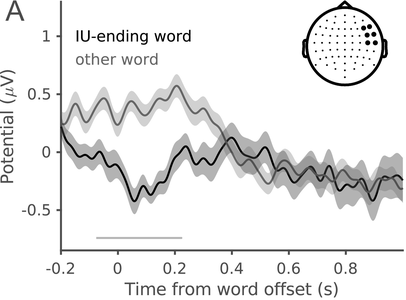
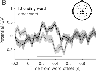
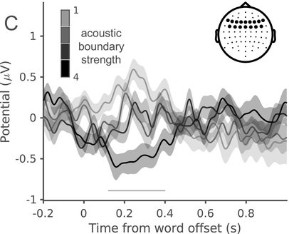
In a recent study, we measured the electroencephalography (EEG) of participants who listened to different speakers recounting an emotional life event in Hebrew (Genzer et al., Reference Genzer, Ong, Zaki and Perry2022; Inbar et al., Reference Inbar, Genzer, Perry, Grossman and Landau2023). We analyzed the stimuli into IUs based on close auditory listening and categorized each word as either ending an IU or not. Additionally, we quantified an acoustically based measure of prosodic boundary strength at each word (see Box 15.1). We modeled the neural response at each EEG channel and time point relative to word offset. We found that the EEG response to words that end an IU differs from the response to words that do not end an IU, even when equating acoustic boundary strength. The EEG response at IU closure includes a negative deflection at right-anterior electrodes, starting shortly before the end of the final word in the IU and lasting circa 200 ms (Figure 15.2A). IU closure is further characterized by a centroparietal positive deflection between 150 and 500 ms after the final word in the IU (Figure 15.2B). In addition, we found that stronger acoustic boundaries elicit a larger anterior negativity between 100 and 400 ms (Figure 15.2C). Thus, when listening to spontaneous speech, the neural system is attuned to IUs. The response to IUs extends beyond a response to mere acoustics and captures processing at higher levels of representation that presumably unfolds in sequences of IUs.
IUs: neural response.
ERP traces in response to words that end an IU and other words with comparable acoustic boundary strength (dark and light gray, respectively), illustrating the right-anterior negative cluster. The traces show the grand average over the EEG electrodes highlighted in the inset topography. Shaded ribbons correspond to ±1 SEM. The horizontal bar marks time points of significant difference between conditions (corrected for multiple comparisons).
ERP traces in response to words that end an IU and other words with comparable acoustic boundary strength (dark and light gray, respectively), illustrating the centroparietal positive cluster. The traces show the grand average over the different sets of EEG electrodes highlighted in the inset topography. Shaded ribbons correspond to ±1 SEM. The horizontal bar marks time points of significant difference between conditions (corrected for multiple comparisons).
ERP traces in response to words that end an IU at different levels of acoustic boundary strength, illustrating the anterior negative cluster. Four different levels are presented, corresponding to quartiles of boundary strength scores within words that end an IU. The darker the gray, the stronger the acoustic boundary. The traces show the grand average over the EEG electrodes highlighted in the inset topography. Shaded ribbons correspond to ±1 SEM. The horizontal bar marks time points of significant difference between conditions (corrected for multiple comparisons).
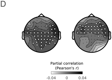
Group average partial correlation maps of the unique predictive accuracy of IU closure (left) and acoustic boundary strength (right), when predicting left-out EEG data in the delta band. Highlighted electrodes denote electrodes in which the predictive accuracy was significantly higher than chance (corrected for multiple comparisons).
Within the ERP literature, previous work has identified a component that resembles the response described in the previous paragraph, the closure positive shift (CPS) (Bögels et al., Reference Bögels, Schriefers, Vonk and Chwilla2011; Steinhauer et al., Reference Steinhauer, Alter and Friederici1999). The CPS was found in response to prosodic phrase boundaries in several languages other than Hebrew, including German, Dutch, English, Swedish, Japanese, Chinese, and Korean. See a detailed account of the CPS in Chapters 17 and 18. Prosodic boundaries in these studies rely on cues that are nearly identical to those defining IUs. Importantly, however, these studies always used isolated, constructed sentences, and so, to the best of our knowledge, our analysis was the first to characterize a CPS-like response to spontaneous speech during naturalistic listening conditions. Furthermore, our modeling approach allowed to address a debate in the CPS literature considering the extent to which the CPS reflects a linguistic structuring of the input beyond the bottom-up response to acoustic boundary cues (Itzhak et al., Reference Itzhak, Pauker, Drury, Baum and Steinhauer2010; Kerkhofs et al., Reference Kerkhofs, Vonk, Schriefers and Chwilla2007; Pannekamp et al., Reference Pannekamp, Toepel, Alter, Hahne and Friederici2005; Pauker, Reference Pauker2013; Steinhauer, Reference Steinhauer2003). Our results suggested what appear to be two different components within the classical CPS. The early- and right-anterior negativity and the centroparietal positivity do not depend on acoustic boundary strength, while the late-anterior negativity is dependent on acoustic boundary strength. This neat result was made possible by combining linguistic theory that focuses on language use with a modeling approach that considers trial-level dynamics among multiple factors.
15.4.2 Brain Rhythms
Research in recent decades has highlighted the relation between temporal structure in speech and temporal structure in brain activity. Understanding this relationship and its role for language has been an influential research program and is one of the goals of the current book. For a detailed presentation of temporal structure in brain activity, see Chapter 3. This line of research suggests that neural activity tracks speech moment by moment (Giraud and Poeppel, Reference Giraud and Poeppel2012; Gross et al., Reference Gross, Hoogenboom and Thut2013; Obleser and Kayser, Reference Obleser and Kayser2019). Neural speech tracking refers to any significant relationship between brain activity and a speech stimulus. Neural speech tracking has been found in different timescales, among them, the theta band (4–8 Hz). This temporal scale is thought to reflect neural tracking of syllables, which across languages tend to have a similar temporal structure: four–eight syllables per second (Chandrasekaran et al., Reference Chandrasekaran, Trubanova, Stillittano, Caplier and Ghazanfar2009; Ding et al., Reference Ding, Patel and Chen2017; Greenberg et al., Reference Greenberg, Carvey, Hitchcock and Chang2003; Pellegrino et al., Reference Pellegrino, Coupé and Marisco2011; cf. MacIntyre et al., Reference MacIntyre, Cai and Scott2022). Neural speech tracking has also been found in the delta band (1–2 Hz); however, in this band there was, until recently, less understanding as to what speech components are being tracked (see detailed discussions in Chapters 17 and 21). From a continuous perspective, since sequences of IUs in spontaneous speech give rise to rhythms of ~1 Hz, the time course of neural responses to IUs is expected to give rise to delta band neural speech tracking. In Inbar et al. (Reference Inbar, Genzer, Perry, Grossman and Landau2023), we showed precisely this. IU-related activity captures previously described delta band neural activity (Figure 15.2D). Specifically, IU-related potentials were able to accurately predict unseen continuous EEG responses to our stimuli in the delta band. This finding was made possible by our analytic approach: We relied on regression ERPs and then used the stimulus parameters and the fitted potentials to predict continuous EEG signals.
Note that Meyer et al. (Reference Meyer, Henry, Gaston, Schmuck and Friederici2016, Reference Meyer, Sun and Martin2020) hypothesized that there may be a link between low-frequency neural speech tracking and the CPS. As discussed briefly in Section 15.4.1, the CPS literature debated to what extent the component reflects a linguistic structuring of the input beyond the bottom-up response to acoustic boundary cues. This debate is also at the crux of the uncertainty relative to speech tracking in the delta band. Thanks to our modeling approach, in which the EEG was regressed against multiple predictors, low-frequency speech tracking could be probed relative to individual predictors while accounting for activity explained away by other predictors. Acoustic boundary cues were found to uniquely predict delta band neural activity in one cluster (Figure 15.2D, right), whereas IU-closure status uniquely predicted delta band neural activity in a separate cluster (Figure 15.2D, left). We also studied the unique contribution of one specific higher-level linguistic representation to delta band neural activity, namely clause closure (see Figure 6 in Inbar et al., Reference Inbar, Genzer, Perry, Grossman and Landau2023). Clause closure also predicted unique delta band neural activity, yet to a lesser extent than IU closure and in a smaller cluster.
The current section has dealt exclusively with IUs in speech comprehension. We discussed IUs in speech comprehension as perceptual units relevant also to higher-level cognitive processes. One might expect that focusing on speech production will be no less illuminating regarding the cognitive processes and underlying neural mechanisms associated with IUs. This topic is beyond the scope of the current chapter, yet we would like to raise a question for future research. Speech production involves an ensemble of motor components, and some have suggested that speech timing might emerge from dynamical interactions between these motor components (Turk and Shattuck-Hufnagel, Reference Turk and Shattuck-Hufnagel2014). Are the motoric facets of IU production the sole contributors of their temporal structure? Conversely, perhaps we might identify additional, higher-level cognitive processes at play, such as the process of selecting what to say in the first place, involving both attention and memory (see Chapter 18).
15.5 Conclusion
This chapter provides a step forward in identifying a promising theoretical construct in the study of cognition, especially within the context of rhythms of language and the brain. We focus on the prosodic organization of spontaneous spoken language into intonation units (IUs). Prosodic chunking into IUs is fundamental to human language. We have presented the phonetic-prosodic definition of IUs and current research regarding their temporal structure. We have discussed the roles of IUs in pacing the flow of information in the unfolding discourse, as revealed in studies of everyday conversation. We have surveyed open questions in the neuroscientific literature that recently benefited from considering IUs in speech: questions pertaining to the nature of the CPS and delta band speech tracking. Finally, we have reviewed algorithmic tools for IU identification to facilitate further investigations relying on this construct. Our approach highlights the importance of studying language mechanisms from the perspective of their use, and applying advanced analytical methodologies for this task.
Summary
Spontaneous spoken language is structured in time at the level of prosodic phrasing, a presumably universal property of language. Linguistic research suggests that this structure offers a window onto dynamic cognitive processes during communication. Neural speech tracking in the delta band is predictable based on the prosodic organization of speech into IUs.
Implications
Considering language in its natural occurrence, that is, communication, has proven crucial for describing rhythm in language and the brain. Future research on the cognitive neuroscience of language will benefit from considering the complexities and richness of the way we use language.
Gains
The chapter introduced key points from linguistic research on IUs, and offered a usage-based approach to the neuroscientific study of language. The chapter further surveyed automatic applications for arriving at a prosodic segmentation of speech. These tools might facilitate investigations on prosodic phrasing and its interface with other domains of language and cognition in ecological settings.
16.1 Introduction
Spontaneous conversational speech appears to be produced in spurts. Rather than being a fluent, uninterrupted flow of words, it is jerky and irregular: Hesitations, false starts, and repetitions are the norm, not the exception (Chafe, Reference Chafe1994; Goldman-Eisler, Reference Goldman-Eisler1961; Shriberg, Reference Shriberg2001). In a technical sense, periods of fluent articulation are intermittent: Speech is comprised of short bursts of articulatory activity interrupted by periods of inactivity. Despite this, it has been suggested that there is a phrasal rhythm of speech, and that an oscillatory mechanism generates this rhythm. This notion might be inspired by the observation that syllables and stress can have fairly regular periodicities, or perhaps from the occurrence of low-frequency neural oscillations phase-locked to syllabic events in speech perception (Chapter 3; Boucher et al., Reference Boucher, Gilbert and Jemel2019; Peelle and Davis, Reference Peelle and Davis2012). But is there evidence for temporal regularity in speech production on longer timescales?
This chapter is organized as follows. First, some empirical data regarding phrase-timescale temporal patterns will be presented. Then, the hypothesis that an oscillatory mechanism directly generates these temporal patterns is considered. Lastly, I present a model in which phrase timing is epiphenomenal: Temporal patterns arise indirectly from mechanisms that govern conceptual-syntactic organization.
To preview the conclusions: Evidence for an oscillatory control mechanism is not so strong. Furthermore, such a mechanism may be implausible from a neurophysiological perspective (see discussion in Meyer et al., Reference Meyer, Sun and Martin2019). Instead, I argue that temporal patterns on phrasal timescales result from the actions of systems that organize conceptual and sensorimotor representations. A model is presented in which phrase-timescale intermittency arises from the reiteration of processes that govern the formation of coherent states among conceptual and syntactic systems. In this model, conceptual and syntactic systems transition back and forth between disordered and ordered states, analogous to repeated rapid-cooling processes. For a variety of reasons, these systems may fail to achieve a sufficiently ordered state, inducing a hesitation. Various control parameters can be manipulated to adjust the rate of hesitation. This mechanism provides a more empirically consistent understanding of phrase-timescale temporal patterns in speech production than oscillator-based models.
There are several important limitations of scope for the reader to make note of. First, this chapter addresses timescales at or greater than the prosodic word – metrical-/stress-related temporal patterns should not be confused with the phrasal ones of interest here. Second, I am concerned with speech that is produced spontaneously. This means that speakers themselves generate the conceptual content, usually in turns with a conversational partner, and that neither initiation nor termination of articulation is cued by an external system such as a metronome or experimental stimuli (of course, the environment along with conversational partners are complex external systems that influence initiation and termination of articulation). Third, I focus on the generation of temporal patterns, that is, the production of speech, as opposed to perception – oscillations in neuronal local field potentials that occur while perceiving speech do not constitute evidence that oscillations govern speech generation (see Chapter 6). Lastly, I do not discuss theories of hierarchical prosodic phrase structure, because prosodic-structural theories do not directly specify mechanisms that generate temporal patterns. Whether such theories could be adapted to do so is an open question (see Chapter 20).
One important terminological point should be made up front regarding use of the term rhythm, which is the topic of this volume. In a generic sense, rhythm can be used to describe any temporal pattern whatsoever. But in this generic usage, the term rhythm lacks bite: All speech has some temporal pattern. I prefer to reserve the term rhythm for the presence of a regular temporal pattern. Most dictionary definitions agree with this qualifier, and many researchers use rhythm to imply some form of temporal regularity in the recurrence of events. For example, Nolan and Jeon (Reference Nolan and Jeon2014) describe a notion in which a pattern must repeat and the temporal intervals of repetition must be regular. Likewise, the original notion of metrical rhythm classes (Abercrombie, Reference Abercrombie1967; Pike, Reference Pike1945) was assessed using direct measures of temporal isochrony in syllables or feet (Lehiste, Reference Lehiste1977; Ohala, Reference Ohala, Fant and Tathm1975). The reason that Turk and Shattuck-Hufnagel (Reference Turk and Shattuck-Hufnagel2013), in their discussion of rhythm, state that speech “is not periodic on the surface … [and] that no constituent recurs at regular temporal intervals” is because regularity is implied by the word rhythm.
When one insists on a notion of regularity for using the term rhythm, it raises an important question: What makes a temporal pattern “regular”? There is no nonarbitrary way to distinguish between temporal patterns that might be interpreted as regular and those that might not. Some specific examples of this problem will arise below. It follows that any answer to the question of whether speech exhibits temporal regularity is subjective – it depends on an arbitrary decision about what constitutes regularity. For this reason, rather than trying to determine the phrasal rhythm of speech, a more productive line of inquiry is to explore what sorts of models can generate empirically consistent patterns.
16.2 Some Empirical Data
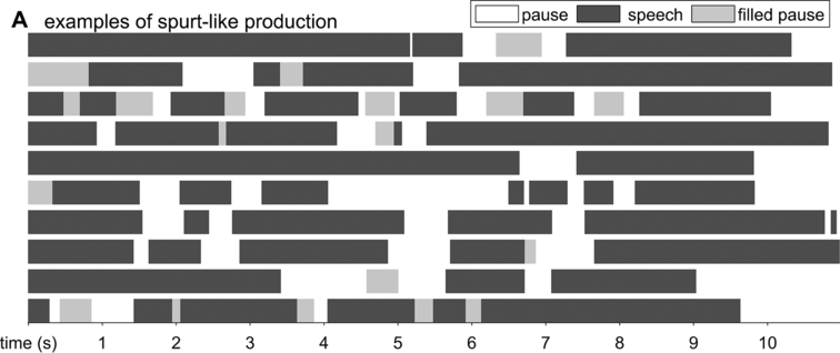
Spontaneous conversational speech is produced in spurts. In more abstract terms, spurts are periods of high activity separated by periods of inactivity. In speech, this means that speakers tend to produce one to several words or phrases and then briefly hesitate or pause. As observed in Chafe (Reference Chafe1994: 57): “Anyone who listens objectively to speech will quickly notice that it is not produced in a continuous, uninterrupted flow but in spurts.” A schematic illustration of the spurt-like nature of speech is shown in Figure 16.1A, which depicts speech activity patterns from 10 relatively long turns randomly selected from the Switchboard NXT corpus (Calhoun et al., Reference Calhoun, Carletta and Brenier2010; Godfrey et al., Reference Godfrey, Holliman and McDaniel1992) (henceforth SWB). Speech and nonspeech periods are shown with dark gray and white intervals, respectively; filled pauses (uh, um) are shown with light gray.
The spurt-like temporal pattern of speech.
Depiction of speech activity intervals from randomly selected conversational turns from the SWB corpus: white is silence, dark gray is speech, and light gray is filled pause.
Markov chain transition probabilities.
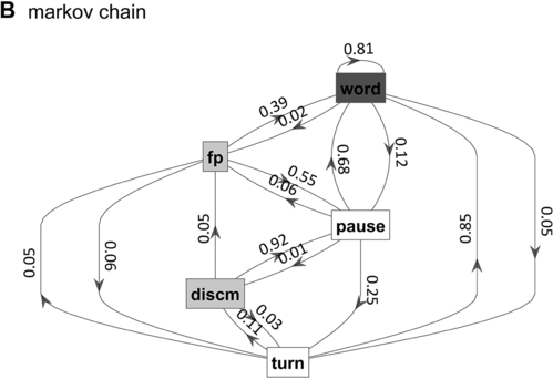
Figure 16.1(B) Long description
The nodes represent the states, and the arrows represent the probabilities of moving from one state to another. The numbers on the arrows indicate the transition probabilities.
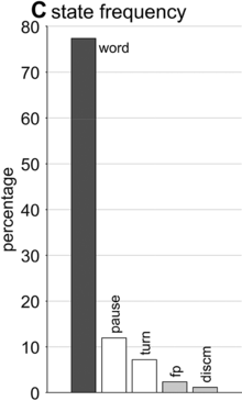
State occupation percentages.
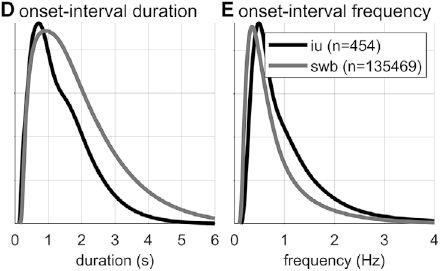
Gaussian kernel densities of unit onset-to-onset duration and frequency from the SWB and IU (intonational unit) corpora.
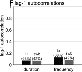
Lag-1 autocorrelations of consecutive interval durations and frequencies.
In a qualitative sense, periods of speech activity in some ways may resemble other natural phenomena that are intermittent, such as firewood popping, the acoustic emission of paper crumpling, or even earthquakes. These are instances of so-called crackling noise, which is associated with a class of systems that exhibit power-law distributions of event sizes or rates (Clauset et al., Reference Clauset, Shalizi and Newman2009; Sethna et al., Reference Sethna, Dahmen and Myers2001). Another natural example of intermittency arises in some circumstances when fluids transition back and forth between laminar and turbulent flow. Even fairly simple dynamical systems such as the Lorentz system can exhibit intermittency, and there are a number of different ways it can arise (Pomeau and Manneville, Reference Pomeau and Manneville1980). In such systems, rate or size distributions are similar across a wide range of scales. However, unlike the above examples, the durations of speech activity periods vary in a range that is no more than two orders of magnitude (i.e., 100–102), and so it is difficult to assess whether these events exhibit a power-law distribution of sizes. Whether or not the physical examples are good analogies to speech is hard to say, since we know so very little about the mechanisms that generate speech.
What is known, however, is that spontaneous speech rarely remains fluent for an extended time. Figure 16.1B shows a Markov model representation of speech-state transition probabilities obtained from the SWB corpus. This model makes the simplifying assumptions that (i) speech activity is always in one of a set of mutually exclusive states and (ii) there are probabilities that the speaker transitions between each pair of states. The model is useful to examine not because it is a realistic model of behavior but because it helps us visualize and quantify the temporal persistence of fluency. Note that due to polysemy, a set of certain words (e.g., yeah, no, okay) were counted as discourse markers when occurring pre- or post-pausally, and otherwise as words (see below for additional methodological details). The transition probabilities of the Markov model show that nearly one out of every five words is followed by something other than a word, such as a pause (12%), a filled pause (5%), or a change of turn (5%). Furthermore, Figure 16.1C shows that the overall occupancy rate of the word state is only about 75% across the corpus. The 0.81 self-transition probability of the word state entails that when a speaker initiates a phrase, there is less than a 50% chance that the phrase will consist of more than three words before being interrupted.
To quantify variability in phrasal temporal patterns, I examine durational patterns associated with periods of fluent speech activity, or spurts. I define a spurt as a sequence of words that does not include a hesitation (pause or filled pause); also, pre-/post-pausal discourse markers are excluded from the analyses, since these are often associated with turn changes. The periods of time between the onsets of consecutive spurts within a turn were extracted from the SWB corpus – here these are referred to as spurt intervals. The frequencies associated with spurt intervals are merely the reciprocals of their durations (see Greenberg et al., Reference Greenberg, Carvey, Hitchcock and Chang2003, for similar and additional methods for analyzing temporal patterns).
Researchers familiar with abstract theories of prosodic structure might wonder: Would it not be better to examine the intervals between onsets of some familiar prosodic units, such as phonological phrases or intonational phrases? The answer to this question could very well be no, since it is not very common for such phrases to be produced without any internal hesitation; moreover, there is no ground truth parsing of speech into higher-level prosodic structure, and there is substantial disagreement about the nature of the structure: Theories range from positing a hierarchy of unique levels (Beckman and Pierrehumbert, Reference Beckman and Pierrehumbert1986; Hayes, Reference Hayes, Kiparsky and Youmans1989; Nespor and Vogel, Reference Nespor and Vogel2007; Selkirk, Reference Selkirk1986), to positing just a couple of levels with recursive organization (Ito and Mester, Reference Ito and Mester2007; Wagner, Reference Wagner2010), to positing no structure whatsoever (Tilsen, Reference Tilsen2019b, Reference Tilsen2022). Nonetheless, for purposes of comparison, Figures 16.1D–F show data associated with intonation units, obtained from the Santa Barbara Corpus of Spoken American English (SBC; Du Bois et al., Reference Du Bois, Chafe, Meyer, Thompson and Martey2000) and manually labeled by Inbar et al. (Reference Inbar, Grossman and Landau2020). I refer to the intervals between intonation units as IU intervals.
Spurt and IU interval durations are highly variable. Gaussian kernel densities of the interval durations are shown in Figure 16.1D for spurt intervals (gray lines) and IU intervals (black lines). Although the distributions do have modal durations (about 0.75 and 1.0 s, respectively), the ranges of the intervals are quite wide: from about 0.5 s to 4 or 5 s. These fairly wide ranges suggest that it may be difficult to accurately predict when the next spurt will begin merely from knowledge of when the current one began. Notice that the distribution of spurt intervals is also skewed rightward, indicating that there are more long spurts than would be expected from a normal distribution of inter-spurt intervals. Figure 16.1E shows effectively the same patterns, after the durations are transformed to frequencies. Note that the modal frequencies do not correspond to the modal durations because Gaussian kernels applied to nonlinearly related variables (such as duration and frequency) do not match.
Furthermore, consecutive spurt/IU intervals are not strongly correlated. Figure 16.1F shows the lag-1 autocorrelations of spurt/IU interval durations and frequencies. The lag-1 autocorrelation is the value of a variable correlated with the next observation of that variable. In other words, lag-1 autocorrelation quantifies to what extent one interval is correlated with the next. This is a useful measure to examine because some of the variability in interval durations may arise from differences across speakers, turns, or contexts – yet these sources of variance should have minimal influence on the correlation of adjacent intervals. Since the lag-1 autocorrelation can only be calculated from consecutive intervals (i.e., three consecutive spurts or IUs), and since some turns are comprised of just one or two spurts/IUs, only a portion of the intervals can be included in the analysis (about 68% and 42% for the two corpora). Notice that lag-1 autocorrelations are positive, but they are fairly small. Even the largest (r ≈ 0.15 for IU frequencies) entails that the frequency of one IU accounts for less than 3% of the variation in the next.
What do the empirical patterns tell us about the regularity of phrasal timing in spontaneous speech? Recall that one fifth of the time a word will be followed by something other than a word, and that 50% of spurts will consist of three words or fewer; these observations call into question whether it is sensible to look for regularity in the first place: If long stretches of speech without pauses, discourse markers, or changes of turn are relatively uncommon, what exactly should one measure to detect phrasal regularity? Second, regarding the duration/frequency distributions of spurt and IU intervals, it is my opinion that the presence of a modal (most common) duration/frequency does not itself constitute evidence for regularity of temporal patterns. Rather, the widths and shapes of the distributions are important: Whereas very narrow, symmetric distributions might support the idea that there are regular temporal patterns, very broad, skewed distributions do not. Some of the variance in the corpus-wide distributions of interval durations/frequencies might be attributed to variation between speakers/turns; in that case, temporal regularity would lead us to expect substantial lag-1 autocorrelations between consecutive intervals within a turn, but this does not appear to be the case either.
There are some potential criticisms of the methodology for obtaining the empirical measures of spurt timing. For one, it was not possible to automatically detect spurt-internal discourse markers and other forms of disfluency (such as cutoffs, repetition disfluencies, or simply hesitatory lengthening while maintaining a speech posture), and so some spurts may be erroneously longer than they should be. However, this criticism does not apply to the manually labeled IU units, which also exhibit high variability and low lag-1 autocorrelation. It also seems unlikely that even if these criticisms could be addressed, interval distributions would become substantially narrower.
Nonetheless, any qualitative interpretation of the patterns is necessarily subjective: How narrow should a distribution be, or how high should an autocorrelation be, in order to infer the existence of a phrasal rhythm? Instead of trying to answer the question of whether the empirical patterns provide evidence for a regular phrasal rhythm, I pursue a related question: What are the necessary properties of a periodic control mechanism that would be consistent with the observed temporal patterns? This is the approach pursued in the next section.
16.3 Oscillation as a Direct Rhythm Mechanism
Here I consider oscillation as a possible generating mechanism for phrasal temporal patterns. Such a mechanism could be motivated from the fact that there is evidence for oscillation on sub-phrasal timescales, that is, timescales of syllables/stress. For example, metrically regular patterns are produced more quickly and with fewer errors than irregular ones (Tilsen, Reference Tilsen2011); in tongue twister paradigms, the reverse pattern holds: More errors occur in metrically regular sequences (Myers and Watson, Reference Myers and Watson2021). Stuttering is diminished in speech entrained to a metronome (Chapter 46; Brady, Reference Brady1971). More generally, cultures have a pervasive habit of putting speech to a beat. There are several models in which oscillatory mechanisms are involved in generating sub-phrasal rhythms (for some examples, see O’Dell and Nieminen, Reference O’Dell and Nieminen1999; Saltzman et al., Reference Saltzman, Nam, Krivokapic and Goldstein2008; Tilsen, Reference Tilsen2009, Reference Tilsen2019a). The fact that oscillation appears to be relevant on the sub-phrasal scale raises the question of whether it is also involved on larger temporal scales, that is, those of phrases.
A number of researchers have developed oscillator-based models of phrasal rhythmicity, but none of these readily applies to the generation of spontaneous speech. For example, there are models of phrasal oscillation in special experimental contexts with metronome-entrained speech (Cummins and Port, Reference Cummins and Port1998; Port, Reference Port2003; Tilsen, Reference Tilsen2009), but there is little evidence to suggest that these models generalize to spontaneous speech. There are also oscillator models that are applied to neural activity evoked in speech perception (Bourguignon et al., Reference Bourguignon, Molinaro and Lizarazu2019; Giraud and Poeppel, Reference Giraud and Poeppel2012; Inbar et al., Reference Inbar, Genzer, Perry, Grossman and Landau2023; Rimmele et al., Reference Rimmele, Poeppel and Ghitza2021), but these do not necessarily claim that oscillations generate phrasal temporal patterns in production, only that such patterns arise in perceiving speech. Notably, although it has been argued that low-frequency delta-band (<1–2 Hz) activity observed in electroencephalography (EEG)/magnetoencephalography (MEG) supports perceptual chunking of phrases, it has alternatively been argued that the low-frequency oscillation arises from pauses in connected speech (Zhang et al., Reference Zhang, Zou and Ding2023). Chapters 3, 5–7, and 9 further address the role of neural oscillation in speech processing. Some recent theories (Benítez-Burraco and Murphy, Reference Benítez-Burraco and Murphy2019; Tilsen, Reference Tilsen2019b) have proposed that oscillations organize neural processes that construct conceptual-syntactic representations, but neither of these holds that neural oscillations are directly responsible for the initiation or termination of motor actions (Chapter 6). There currently exists no implemented model of phrasal oscillation in spontaneous speech.
16.3.1 Empirical Evidence for Phrasal Rhythmicity
To my knowledge, there are just two studies in the literature that use empirical evidence to support the claim that phrasal rhythms in production are associated with an oscillatory mechanism. One of these is a recent study of IUs (Inbar et al., Reference Inbar, Grossman and Landau2020). The authors examined manually labeled IUs from spontaneous speech in a variety of languages, including the SBC (included in the analyses above). To investigate temporal patterns, they conducted a clever analysis using a phase consistency measure developed for studying neural oscillations (Vinck et al., Reference Vinck, van Wingerden, Womelsdorf, Fries and Pennartz2010). The analysis works as follows (see Chapter 15). First, a wideband amplitude envelope of the speech signal is split into two-second windows centered on the onset of each IU, and these windows are Hann-windowed. Then a Fourier transform is applied to each window, and the consistency of the phase of each complex Fourier coefficient component is calculated by the pairwise phase consistency (Vinck et al., Reference Vinck, van Wingerden, Womelsdorf, Fries and Pennartz2010). This value is effectively an average angular correlation between the phases estimated from all windows, for a given frequency component. Intuitively, this measure tells us how similar the phases of a particular Fourier component are across a dataset. Inbar et al. (Reference Inbar, Grossman and Landau2020) found that there was a peak in the consistency around 1 Hz (note that two-second windows entail effective frequency bins of 0.5 Hz, which are wide in relation to the typical durational range of IUs). They interpret this finding by stating that “prosodic units … give rise to a low-frequency rhythm” and that “speakers express their developing ideas at a rate of approximately 1 Hz.” These statements seem to suggest that a phrasal oscillation governs speech production, although it is unclear whether the authors contend that organization into IUs is the cause or effect of the phrasal rhythm.
There are several potential criticisms of the Inbar et al. (Reference Inbar, Grossman and Landau2020) study that call into question how strongly it supports the idea that there is a phrase-timescale oscillation that governs speech. First, the pairwise phase consistency analysis method they used is more complicated than the simpler method of examining the distributions and autocorrelations of interval durations/frequencies; if these simpler methods show broad distributions, then the discrepancy between methods warrants an explanation. Second, the manual labeling of IUs makes a presupposition about the existence of such units; this presupposition cannot be independently validated from a ground truth parsing of the signal because the units themselves are hypothetical entities (Chafe, Reference Chafe1994). Third, since the analysis considers all windows, it represents an aggregate over speech produced at different times and from different speakers, as opposed to a temporally local correlation between successive intervals. Fourth, and most importantly, the interpretation of the presence of a peak in phase consistency suffers from the same problems of subjectivity and arbitrariness that were discussed above in relation to interval duration distributions: The width and shape of the distribution must also be considered, not just the presence of a mode. In my estimation, the phase consistency functions for each of the six languages examined in Inbar et al. (Reference Inbar, Grossman and Landau2020) are not very sharply peaked: The half-bandwidths of the peaks in most cases appear to extend from approximately 0.25 to 2 Hz (or, 4 to 0.5 s), which is a fairly broad range. Indeed, the results could very well be interpreted as evidence against temporal regularity on the phrasal timescale.
A second study that also argues for a phrasal oscillation is Stehwien and Meyer (Reference Stehwien and Meyer2022). The authors examined human-annotated intonational phrases and intermediate phrases from a corpus of German radio news. They conducted autocorrelation analyses on subsets of data in which intonational phrases were collected according to their durations, using one-second bins. The autocorrelation was conducted on binary time series with time steps of 0.001 s, in which the value 1 indicated the offset of an intermediate phrase. Using this approach, they found significant autocorrelation at lags in the range of 610–1,200 ms – a frequency range of 0.83–1.64 Hz. They also report that the standard deviation of differences in adjacent phrase durations was 1.11 s. Stehwien and Meyer (Reference Stehwien and Meyer2022) interpret the findings as “evidence for an association between acoustic patterns in speech and periodic electrophysiological sampling time windows of the auditory system” – this association might be taken to imply that auditory oscillations are responsible for periodicity in the acoustic output of speech (although the authors do not explicitly state this).
Some of the same criticisms that bear on Inbar et al. (Reference Inbar, Grossman and Landau2020) apply to Stehwien and Meyer (Reference Stehwien and Meyer2022). Specifically, the intonational and intermediate phrase parsings are contestable because they are hypothetical units, and most importantly, it is not clear whether the frequency range of significant lags (0.83–1.64 Hz) should be viewed as relatively narrow or relatively broad. The phrase-to-phrase jitter of 1.11 s indeed seems to be quite large. Furthermore, it is important to note that analyses of broadcast news speech may not generalize to spontaneous speech: Broadcast news speech is produced by speakers with specific training, it is often guided by a transcript, and it may have its own stylistic characteristics, including context-specific intonational patterns.
16.3.2 Assessment of a Model of Oscillator-Driven Phrasal Timing
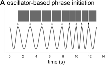
To further assess the idea that phrasal timing patterns can be explained by an oscillatory mechanism, one can explore the predictions of an oscillator-based model. Because there is no well-developed spontaneous speech phrasal oscillator model in the literature (see Chapter 6), it is necessary to borrow an idea from the metrical oscillator models. A typical aspect of these models is that the initiation of a syllable/foot is triggered when the oscillator reaches some particular phase of its cycle (see, for example, Saltzman et al., Reference Saltzman, Nam, Krivokapic and Goldstein2008; Tilsen, Reference Tilsen2009). In other words, the oscillator initiates the production of a unit at some particular moment that is consistent from one cycle to the next. Applying this idea to a phrasal oscillator entails that the reciprocal of a spurt interval (or whatever interval one might define) should correspond to the frequency of the oscillator, as shown in Figure 16.2A. I will assume that the oscillator has a constant frequency within each cycle (note, this assumption does not sacrifice generality because a constant frequency can be viewed as an average of instantaneous frequency over one cycle). Given these assumptions, can an oscillatory mechanism generate the empirical interval densities?
Analysis of a phrase oscillator model.
Schematic illustration of phrase initiation in a phrasal oscillator model.
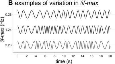
Examples of phrasal oscillation for extremal and medial values of δf-max.
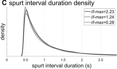
Spurt-interval densities for the extremal/medial values of δf-max.
Lag-1 autocorrelations as a function of δf-max.
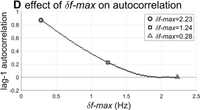
A crucial model parameter to consider relates to how much one will allow the oscillator frequency to vary from one cycle to the next. This parameter is expressed here with δf-max, the maximal absolute change in frequency from one cycle to another. Figure 16.2B contrasts phrasal oscillators with three different values of δf-max, that is, different degrees of time-varying random frequency variability. Low values of δf-max result in fairly regular oscillations, high values in irregular oscillations. Consider that if δf-max is unbounded, oscillator frequency can change arbitrarily from one cycle to another, and the model is overly powerful: It can generate any imaginable pattern of jitter in phrasal intervals. Indeed, allowing for large δf-max seems to subvert the meaning of regularity and periodicity that is associated with the concept of “oscillation.”
What value of δf-max is most consistent with the empirical data? To answer this question, some additional details of the model must be fleshed out. Specifically, a strategy is needed for determining how f changes from one cycle to the next. Here the change is modeled as a random walk, but boundary constraints [fmin, fmax] that correspond to the 5th and 75th percentiles of empirical spurt frequencies are imposed. This means that for each cycle i, a value δfi is randomly selected from the interval [−δf-max, +δf-max], and is added to the frequency of the previous cycle, that is, fi = fi-1 + δfi. If the resulting value falls outside of the bounds [fmin, fmax], a new random value is selected until the resulting frequency is within bounds. In model simulations, 101 values of δf-max were examined, ranging from fmin to fmax. For each value of δf-max, 10,000 consecutive intervals were generated. This Monte Carlo approach to modeling phrasal rhythm provides a time series of adjacent spurt durations, from which lag-1 autocorrelations can be calculated.
The interval duration densities (n=10,000) associated with low, high, and intermediate values of δf-max are shown in Figure 16.2C. The densities show that δf-max does not have a substantial effect on the shape or width of the expected distribution of interval durations. The reason for this is that the random walk eventually explores the entire space between the frequency bounds; it merely does so more quickly with larger δf-max. It is noteworthy that the shapes of the duration distributions are skewed rightward, not unlike the empirical ones (solid black line). In contrast to the frequency distributions, δf-max has a strong effect on lag-1 autocorrelation, shown in Figure 16.2D. Here one can see that a large δf-max of around 1.35 Hz is needed to generate the fairly small empirical lag-1 autocorrelation of r = 0.15.
Overall, the model simulations suggest that in order for a phrase oscillator to generate lag-1 autocorrelation patterns that match the largest values observed in the corpora, then δf-max would need to be around 1.35 Hz. Can this value be interpreted as support for or against the hypothesis that a phrasal oscillator drives phrase initiation? To me, the value seems to allow a fairly drastic change in frequency from cycle to cycle – about 70% of the allowed frequency range (or 24% of the period range). In any case, without a specific model of the neural mechanisms that give rise to the oscillation, it is hard to assess how realistic this variation would be.
There are of course several potential criticisms of the model, which might call into question how strongly inferences can be drawn from it. One criticism might be that stochastic effects in the triggering of phrase initiations are not included; perhaps there is a variable delay from the triggering phase to phrase initiation. Including a random delay would allow for lower δf-max to attain empirically observed autocorrelations, but the magnitude of this random deviation would need to be quite large. Perhaps the most important criticism is that it is too strong to assume that every cycle of oscillation generates a spurt – maybe spurt initiations can skip cycles if the preceding spurt has not been completed. To implement a model of that sort, additional mechanisms would be needed to govern spurt termination. I leave the exploration of this larger parameter space to future work. Nonetheless, the main conclusion from the simulations is that a phrasal oscillator would seem to need an overly powerful ability to change frequency in order to generate empirically consistent temporal patterns.
The second reason why direct oscillatory control of phrasal timing may not be plausible is a neurophysiological one: The frequency range necessary to account for empirical interval distributions is unlikely to be associated with a single neurogenic origin. It seems reasonable to expect that if there exists a phrasal oscillator, its neural origins would have a unitary origin. Our current knowledge of how neural oscillations arise may not be consistent with this expectation. Consider that even a very conservative estimate of the range of IU frequencies from the SBC corpus is about 0.25–2 Hz. Although occasionally one can find superficial descriptions of neural oscillation frequency bands in which this range of values is labeled as δ-band (delta-band), many of the more detailed analyses distinguish between different delta bands, due to the fact these have different apparent origins and behavioral correlates. There is in fact no widespread agreement about the functions of different oscillations in different bands. For instance, Buzsáki and Draguhn (Reference Buzsáki and Draguhn2004) distinguish between delta (1.5–4 Hz), slow 1 (0.5–1.5 Hz), and slow 2 (0.20–0.5 Hz) oscillations. Or, Jensen et al. (Reference Jensen, Spaak, Zumer, Supek and Aine2019) describe delta as (1–4 Hz) and note that a proposed neurogenic mechanism involves slow inhibitory neurotransmitter effects in cells that project from the thalamus to the cortex, which form part of a thalamo-cortical circuit. Other oscillatory bands, such as theta, alpha, beta, gamma, and high gamma, are each proposed to arise from different mechanisms. To my knowledge, no one has proposed that there exists a functionally coherent 0.25–2 Hz band of oscillatory activity with a single neurogenic mechanism (see also Chapters 3 and 35). Moreover, it is a bit puzzling that the strongest delta rhythms tend to be observed during sleep (Buzsáki and Draguhn, Reference Buzsáki and Draguhn2004). Thus, one should be cautious in jumping to the conclusion that just because there is oscillatory neural activity across a range of low frequencies, it supports the notion of a phrasal oscillator.
16.4 Conceptual-Syntactic Coherence as the Source of Phrase-Timescale Temporal Patterns
Instead of thinking of phrasal timing as something that is controlled directly, perhaps phrase initiation can be understood as an indirect consequence of other control mechanisms, namely those that are involved in conceptual and syntactic processes. In other words, perhaps speakers do not care at all about when phrases are initiated: There is no system that directly governs phrasal timing.
In this section I describe a theoretical framework for understanding speech production – the oscillators and energy levels framework – developed in Tilsen (Reference Tilsen2019b). Then I present simulations of a model in this framework, in which there are mechanisms that give rise to intermittency of speech activity. Finally, I explain how this model can be used to describe transitions to and from fluent speech. The key ideas of the model are that there are special systems that monitor the states of conceptual and syntactic systems; and furthermore, whenever conceptual and syntactic systems reach a noncoherent state, these monitoring systems induce a reorganization process that results in hesitation, that is, a temporary halt of content-related speech activity. The notion of coherency of state may be unfamiliar to readers and is elaborated and exemplified below.
Section 16.4.1 provides a highly condensed overview of some of the basic aspects of the oscillators and energy levels theory, which is too large in scope to describe in its entirety here. Section 16.4.2 shows with model simulations how intermittency can arise. Only the most relevant details are made explicit here, and the reader should view this section as a proof-of-concept, as opposed to a comprehensive presentation of the model. For readers who are interested in the details of the model, a full exposition of all parameters, equations, model code, and examples of how to run the model are available at https://github.com/tilsen/oel_intermittency.git.
16.4.1 Overview of the Parallel Domains – Oscillators/Energy Levels Theory
In the oscillators/energy levels theory, all entities involved in speech production are dynamical systems with the potential for oscillatory activity; their states can be described by variables of phase, instantaneous frequency, and amplitude. There are two primary domains of organization: the conceptual-syntactic domain (cs-domain), and the gestural-motoric domain (gm-domain). These are referred to as parallel domains for two reasons: (i) system states in both domains evolve at the same time and (ii) the mechanisms of organization in the two domains are highly similar. Figure 16.3 illustrates various aspects of the model that are discussed below.
Overview and example of the oscillators/energy levels model.
The example utterance is Allie drinks coffee, Bubba drinks tea. (A) Concept systems couple with syntactic systems, which organize them into relative phase configurations (Aʹ) that describe patterns of oscillation (Aʹʹ). (B) Gestural systems couple with motor-sequencing systems, which organize them into relative phase configurations (Bʹ) that describe patterns of oscillation (Bʹʹ). (C1, C2, C3) Activation potentials for a sequence of states of conceptual-syntactic organization. (D1, D2, D3) Activation potentials for a sequence of states of gestural-motoric organization. (E) Activation variable trajectories for conceptual-syntactic systems. Relative energy hierarchies are indicated. (F) Activation variable trajectories for gestural-motoric systems.
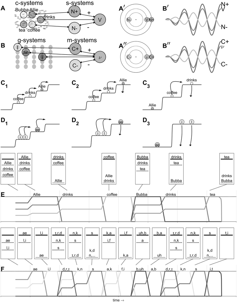
Figure 16.3 Long description
Panel a. A network-like diagram shows relationships between different entities like Bubba, Allie, drinks, tea and coffee. The N plus and N minus symbols and "V" suggest a possible concept of positive and negative influences or states. Panel b. A similar waveform structure is labeled N plus, V, N minus, C plus, C minus and nu. Panel c. Three diagrams show transitions between states, with arrows indicating the direction of change. The entities like Allie, drinks and coffee are involved in these transitions. Panel d. These diagrams are similar to panel C. Panel e. A three-step line representation of words including Allie, drinks, coffee, bubba, drinks and tea. A table shows a sequence of states. The states are denoted with letters including a e, l, i, r, d, n, k, s, k, a, i, f, uh and b, a representing different states. Panel f. A multistep line representation depicts the progression of states, including a e, l, i and more.
In the conceptual-syntactic domain, there are many instantiations of two basic types of systems: concept systems (c-systems) and syntactic systems (s-systems), as represented in Figure 16.3A. Instances of both types are argued to correspond to neural populations. In the case of c-systems, the neural populations that instantiate a particular c-system are distributed across cortical multimodal association areas and interact with primary sensory and motor areas. An example of a c-system is [COFFEE]. This system interacts with various sensorimotor information that encodes, for example, the smell and taste of coffee, its visual appearance, and motor patterns that we have for interacting with it. The neural populations that instantiate [COFFEE] are also expected to overlap with populations associated with related concept systems, such as [TEA] or [CUP]. Because of this, there are varied, diverse interactions between c-systems. Note that there are important differences (as discussed in Tilsen, Reference Tilsen2019b) between c-systems that are more grammatical in nature (such as a c-system for [SINGULAR] or [3RD PERSON]) and those that are more lexical (such as [COFFEE] or [DRINK]) – I will not delve into these aspects of the theory here (see Chapter 6 and Shattuck-Hufnagel, Reference Shattuck-Hufnagel and Redford2015, for alternative perspectives).
Syntactic systems (s-systems), in contrast to c-systems, are neural populations that are more cortically localized and that interact in highly constrained ways. S-systems are defined in part by how they phase-couple to other s-systems. For example, in the production of a simple subject-verb-object (SVO) sentence such as Allie drinks coffee, the subject system (N+) and the verb system (V) are attractively phase-coupled, while the object noun system (N−) and verb system are repulsively phase-coupled. This pattern is shown in the network structure of Figure 16.3A and the resulting relative phase configuration is shown in Figure 16.3Aʹ, with corresponding oscillations in Figure 16.3Aʹʹ. Importantly, c-systems can phase- and amplitude-couple to s-systems, and because of this property, s-systems can organize c-systems into stable relative phase configurations. The relative phase configurations that arise between c-systems indirectly in this way are held to evoke relational meaning experiences. In other words, the meaning of Allie drinks coffee is an experience associated with a particular relative phase configuration. Crucially, this experience is argued to arise when the relevant systems exhibit strong phase coherence, meaning that their relative phases are relatively stable over time.
Similarly, in the gestural-motoric domain, there are two types of systems: gestural systems (g-systems) and motor-sequencing systems (m-systems), as shown in Figure 16.3B. G-systems are similar in some respects to the gestures of articulatory phonology (Browman and Goldstein, Reference Browman and Goldstein1992), but note that in Figure 16.3, for visual simplicity phonetic symbols are used to refer to oral articulatory gestures. In the same way that s-systems organize c-systems into stable relative phase configurations, motor-sequencing systems (m-systems) couple to g-systems and thereby bring them into particular configurations. In this domain, rather than evoking meaning experiences, relative phase configurations dictate coordinative relations between gestures. M-systems also function to group g-systems into sets that are sequentially selected, as theorized in the selection-coordination theory of speech production (Tilsen, Reference Tilsen2014, Reference Tilsen2016). Importantly, the mechanisms that govern c- and s-system interactions in the conceptual-syntactic domain are highly similar to those that govern g- and m-system interactions in the gestural-motoric domain.
All four types of systems can be characterized by two state variables: phase (φ) and activation (or its discrete counterpart, excitation [e]). The dynamical laws that govern these variables depend on which dynamical regime a given system is in. There are three regimes that are distinguished: (i) an inactive state, in which a system is effectively ignored because its excitation variable is too low; (ii) an active state, in which a system exhibits non-negligible but nonetheless low levels of excitation and relatively incoherent oscillation; and (iii) an excited state, in which a system obtains high levels of excitation and exhibits relatively self-coherent oscillation – that is, an oscillation with stable frequency and amplitude. Coherence in this sense can be quantified via autocorrelation: When a system oscillates with stable frequency and amplitude, there will be a strong peak in its short-time autocorrelation, or equivalently a large peak in its power spectrum.
The roles of the three regimes can be understood by considering what happens prior to initiation of speech, and continuing through fluent production. Figure 16.3 panels C1–C3 illustrate activation potentials for the first three epochs of conceptual-syntactic organization in the production of the utterance Allie drinks coffee, Bubba drinks tea; likewise, panels D1–D3 illustrate the potentials for the first three epochs of gestural-motoric organization. (Note that the step functions shown in the panels can be viewed as potentials in the technical sense: They are functions of system activation and the negative of their first derivative is the force that acts on the system; however, the step functions shown here are designed primarily for illustrative purposes rather than quantitative accuracy.) The lowest level of the potential is the ground level – systems that occupy this level are in an active state but are not excited. Systems occupying all above-ground levels are excited. The highest level of the potential is the selection level – c-systems that occupy the selection level exert strong forces on associated g-systems, and g-systems that occupy the selection level exert strong forces on vocal tract systems (which are roughly equivalent to the tract variables of task dynamics [Saltzman and Munhall, Reference Saltzman and Munhall1989]).
In panel C1, the three c-systems of the first clause ([Allie], [drinks], and [coffee]) are initially organized into a relative excitation hierarchy that corresponds to the order in which they will be selected. Other c-systems that may be involved in the utterance are active but not yet excited. The most highly excited system [Allie] is not yet at the selection level. The arrows in C1 indicate what happens after the configuration in epoch C1 stabilizes: [Allie] is promoted to selection level, and the remaining systems [drinks] and [coffee] are promoted to the next highest level, as shown in C2. The arrows in C2 indicate what happens next: When feedback (either internal or external) regarding the selection of [Allie] reaches a threshold, [Allie] is demoted to ground level and the remaining systems are promoted. The demotion of selected systems and the promotion of remaining systems iterate until the next clause, where [Bubba], [drinks], and [tea] are organized and undergo a similar sequence of operations.
Similarly, in panel D1, three gestural systems associated with [Allie] are organized into a relative excitation hierarchy with all three systems initially below the selection level. This organization process is understood to happen contemporaneously with the organization of the c-system [Allie]. Notice that [l] and [i] occupy the same level of the excitation hierarchy. This reflects the observation that these oral gestures will be selected together and coordinated (i.e., co-selected; see Tilsen, Reference Tilsen2016). (Note that c-systems can also be co-selected, and that the system labeled [drinks] in C1–C3 is more precisely understood as a co-selection of the c-system [drink], [3RD PERSON], [SINGULAR], and [PRESENT TENSE].) The arrows in D1 indicate what happens next: The systems associated with [ae] (a lingual gesture and a glottal adduction gesture) are promoted to selection level, as shown in D2, and this drives changes in vocal tract systems/effectors. Eventually, internal and external feedback lead to the demotion of [ae] and the promotion of the next set of gestures, resulting in the excitation configuration shown in D3.
The entire sequence of conceptual-syntactic and gestural-motoric epochs and corresponding activation trajectories for the utterance Allie drinks coffee, Bubba drinks tea are represented in Figure 16.3, panels E and F, respectively. The activation trajectories are idealized representations of the activation state variables of the c- and g-systems over the course of producing the utterance – note that when adopting this quantized representation, activation is relabeled excitation. Discrete epochs of the c- and g-system relative excitation hierarchies are shown above the activation trajectories. The top-most line in each epoch is the selection level; the bottom solid line is the ground level.
The sequence of relative excitation states that occurs in the course of producing an utterance such as the one above can be understood as a dynamical production trajectory: It describes the trajectory of a complex system (consisting of many component systems) in a high-dimensional space, with those systems evolving according to change rules that incorporate force-like interactions between systems and an environment.
The above exposition provides a highly condensed description of the oscillators/energy levels theory (see Tilsen, Reference Tilsen2019b). The key idea for current purposes is this: Before a system can be promoted to selection level, its state has to become relatively stable and coherent. This applies both to the epoch in which systems are initially organized below selection level and to subsequent epochs in the production of the utterance. Specifically, coherence entails that there is a relatively strong peak (or multiple strong peaks) in the autocorrelation or power spectrum of the system state; this will only be present when the system frequency and amplitude are relatively stable.
Loosely speaking, the model holds that prior to utterance initiation, there is a pandemonium of disorganized and unstable oscillation among c-systems and s-systems (i.e., the short-term power spectra of these systems lack clear peaks). Through competitive interactions between systems, the disorganized state rapidly organizes into a highly ordered one in which a small set of c-systems and s-systems exhibit coherent oscillations. This evolution of the full system can be conceptualized as a cooling process. Special-purpose coherence-monitoring systems recognize the achievement of this high degree of coherence and induce processes that result in the generation of movement (which is controlled through similar processes involving gestural and motoric systems). Transitions from disordered, noncoherent states to ordered, highly coherent states occur repeatedly throughout spontaneous speech production.
16.4.2 How Intermittency of Phrase Initiation Arises
This section presents simulations of a model in the oscillators/energy levels theoretical framework. The aim of the model is to show one possible mechanism by which the intermittency of speech activity might arise. The model is intended to illustrate this particular mechanism, rather than generate the statistics of speech activity periods. Nonetheless I will discuss how the model could be used to do this.
The key idea of the model is that hesitations in spontaneous conversational speech can occur when conceptual-syntactic or gestural-motoric configurations become noncoherent (or, degenerate). When this happens, the system resets itself and the speaker hesitates. For simplicity, the model simulates only concept (c-) and syntactic (s-) system states; gestural/motoric organization would exhibit similar sorts of behaviors. Note that model code, descriptions of all model equations and parameters, and examples of how to use the model are available online (https://github.com/tilsen/oel_intermittency.git).
One key point to make about the model is that it requires a surroundings (or “environment”), which is what causes c-systems to become active in the first place (c-systems can also cause other c-systems to become active, but this never occurs in a vacuum). In any real context, the environment is always complex and dynamic, and therefore the forces that c-systems experience will vary in complicated ways over time. In the simulations below, these environmental forces are simplified by making them constant throughout an utterance, yet randomly determined from one simulation run to another. Moreover, a condition is imposed that the utterance is always a SVO sequence. This condition does not sacrifice the generality of inferences about intermittency; it merely serves to allow for more direct comparisons of model behavior as certain parameters are varied.
A second key point to make is that there are a number of sources of stochasticity in the model, and that these are ultimately responsible for the (non)occurrence of degenerate states. Specifically, degenerate states occur when s-systems fail to attain a relative excitation configuration with certain properties. Those properties are, first, that mutually exclusive s-systems cannot occupy the same level of the relative excitation potential, and, second, that there should not exist an unoccupied level of the potential. These circumstances can arise from stochasticity in initial conditions, from interactions between c-and s-systems, or from environmental forces. Furthermore, the forces that are associated with the excitation potential are modulated by an annealing system: These forces are initially weak but strengthen over time. The annealer state is analogous to inverse temperature in that regard, and the formation of a coherent state can be viewed as a cooling process. By increasing the strength of excitation potential forces in this way, there is a period of time when stochastic forces on s-systems may or may not prevent them from coming to occupy the excitation levels in a canonical way. Similarly, whenever a selected system is demoted, there is an annealing process that again allows for stochastic effects on excitation organization.
Some examples of these phenomena are exemplified in Figure 16.4 below. Panels A–C show selected system state variables from several example utterances. In each panel, the top portion shows the activation states of the three s-systems in the utterance (N+, V, N-), and the bottom portion shows the states of the s-system annealer (dashed line) and the excitation coherence monitor (solid line). Example A shows system state trajectories when no degeneracy occurs. Notice that the s-system excitations grow initially but soon stabilize in separate wells of the excitation potential. Subsequently, when the excitation coherence monitor reaches a threshold value (around the time indicated by the arrow), it induces a reorganization of the excitation potential, such that each s-system is promoted. The next reorganization occurs when feedback for the selected syntactic system reaches a threshold value. Iterated reorganizations consist of demoting a previously selected system to the ground level, and promoting all remaining above-ground systems.
Simulations of the intermittency mechanism and parameter effects.
Panels A–C show (top) syntactic system activation trajectories for three syntactic systems and (bottom) annealer (dashed line) and monitor trajectories (solid line).
Canonical production trajectory.
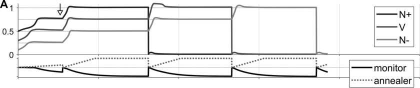
Degenerate excitation state occurring before initial coherence, occurring at the time indicated by the arrow.
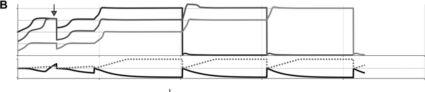
Degenerate excitation state occurring within sequence production, occurring at the time indicated by the arrow.
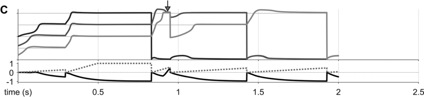
Effects of initial cooling rate and reorganization cooling rate parameters on the likelihood of disfluent initiation and sequencing.
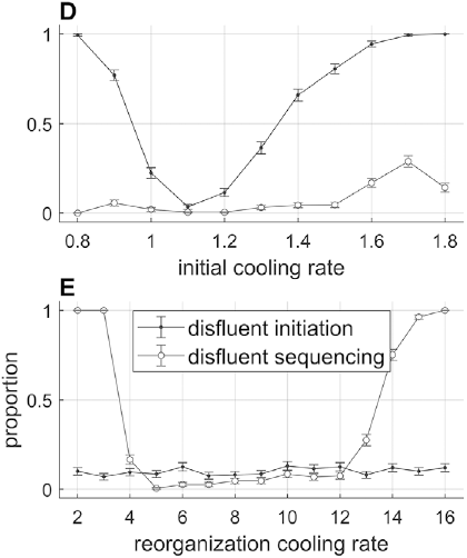
Figure 16.4(D, E) Long description
Graph D plots the disfluent proportions versus initial cooling rate. The initiation line originates at (0.8, 1), falls, and rises to terminate at (0.8, 1.8), and the sequencing line originates at (0.8, 0), fluctuates and terminates at (1.8, 0.2). Values are estimated. Graph E plots the disfluent proportion versus the reorganization cooling rate. The line for disfluent sequencing initially falls, remains stable and then rises. The line for disfluent initiation remains stable along the x-axis.
Effect of concept–concept activation-coupling strength on disfluency likelihoods.
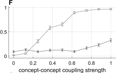
Effect of the number of environmentally excited concept systems on disfluency likelihoods.
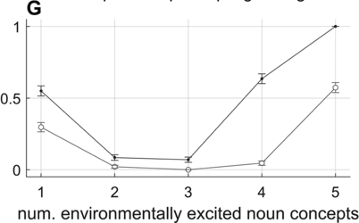
Examples B and C show two different cases in which a degenerate excitation configuration arose in a simulation, at the time indicated by the arrows. B is an example of noncoherence in initiation, or disfluent initiation. Here the degenerate state occurs before the first selection: Both {N+} and {V} occupy the same energy level. The detection of the degenerate state by the monitor induces a reset of s-system activation and a restart of the annealing process. This case corresponds to a hesitation before the initiation of a phrase. C is an example of intra-sequence noncoherence, or disfluent sequencing. Here the degeneracy occurs after the demotion of the first selected system, before {V} is promoted to selection level. The monitor decreases the activation of the above-ground systems and the annealing process is restarted. This case corresponds to a hesitation within a phrase.
Various model parameters influence the occurrence rates of disfluent initiation and disfluent sequencing; moreover, these parameters can be given behavioral/functional interpretations that allow for the model to generate a variety of phenomena. Selected parameter effects are shown in Figure 16.4, panels D–G. Panel D shows that when the initial cooling rates are too high or too low, sequence initiation is more likely to be disfluent. The likelihood of disfluent sequencing (assuming that initial coherence occurred) is mostly unaffected by the initial cooling rate, but note that it increases a bit with high initial cooling rates. Similarly, panel E shows that reorganization cooling rates that are too low or too high lead to disfluent sequencing. The initial cooling rate parameter can be interpreted as the degree of motivation that a speaker has to begin speaking. The model suggests that the more urgency speakers feel to initiate an utterance, the more likely they are to hesitate when trying to begin the utterance. The reorganization cooling rate parameter can be interpreted as a speech rate control parameter: Higher cooling rates produce faster speech, but are more likely to result in disfluency.
Panel F shows how fluency depends on the strength of activation-coupling forces between concepts. Note that concept–concept activation interactions are randomly selected values on the interval [−1,1] with symmetric sign, reflecting the notion that concept interactions are mutually excitatory or inhibitory but generally asymmetric in strength. When these interactions are increased in strength, c-systems are more likely to interfere with each other; this can prevent the achievement of a stable s-system configuration because of c-s activation coupling. Panel G shows how fluency depends on the number of environmentally excited noun concepts. When this number is less than the number required for an SVO utterance, disfluency rates are higher. Conversely, when the number increases, there is greater interference with s-systems and disfluency rates increase. These effects connect with the idea that, like humans, the model has limited working memory.
In sum, the model provides proof-of-concept that the intermittency of speech activity may derive from factors that influence whether conceptual and syntactic systems are likely to organize into states with particular properties. Moreover, the model provides a number of parameters that can be plausibly related to forms of behavioral variation, such as speech rate, as well as contextual variation, such as the number of concepts that are activated by the environment. Importantly, the model shows how we might more realistically conceptualize phrasal timing: Rather than being governed directly by an oscillatory mechanism, temporal patterns on phrase timescales are indirect consequences (epiphenomena) of processes involved in conceptual-syntactic organization.
Before concluding, it is worth discussing a number of shortcomings of the model in its current implementation. First, the excitation dynamics are implemented with discrete operations, but a more sophisticated model would allow for such dynamics to emerge from interacting dynamical systems, or from a spatial organization of systems (e.g., see Grossberg, Reference Grossberg1987). The premise that speech can be idealized as a sequence of discrete operations on states is useful but ultimately needs to be derived from more fundamental systems. Second, in order to achieve coherent initial states, s-systems in the model cannot have arbitrary initial excitation values. Thus, it must be assumed that there exists some mechanism that constrains initial s-system values to certain ranges. Third, the model presupposes that the environment fully determines a particular syntactic configuration. In other words, the canonical syntactic form of an utterance does not emerge stochastically from the state of the environment. Fourth, not only excitation but also relative phase configurations should also be monitored for coherence, and relative phase degeneracies should introduce hesitations. Extensions of the model to address these limitations are currently underway. Once these environmental forces are modeled appropriately, it will be possible for the model to generate conversational turn-timescale output with speech-like intermittency statistics.
Summary
In spontaneous conversational speech, phrases are initiated intermittently. Evidence for an oscillatory mechanism that directly controls phrasal timing is inconclusive. Instead, intermittency in phrasal timing may be an epiphenomenon of processes involved in conceptual-syntactic organization. The sources of intermittency could derive from systems that monitor the coherence of conceptual and syntactic systems.
Implications
Without appropriate controls, statistical characterizations of phrasal timing patterns are unlikely to shed light on the nature of speech production in spontaneous conversational speech. It is crucial to consider syntactic and conceptual factors in phrasal timing. Furthermore, speaker- and discourse-context-related factors must also be considered.
Gains
Our understanding of speech production has been improved by recognizing that the timing of phrases depends on many factors, some of which relate to the conceptual content and syntactic organization of speech. We can avoid mistakenly attributing phrasal timing patterns to the effects of a dedicated control mechanism.
17.1 Introduction
Spoken language is a complex and intricately structured physical signal. Its rich variation stems from a myriad of sources, which are not easily decomposable into discrete variables. What is more, many of these sources of information are related, yielding correlations in the speech signal that are difficult to disentangle experimentally. For spoken language processing, however, this redundancy might actually prove to be valuable, because it enables the brain to leverage one feature to draw inferences about another feature, thereby facilitating comprehension. What seems like an annoying property from an experimental perspective might be an integral condition for perceptual inference.
To give a key example, the structures of syntax and prosody are related, due to which syntactic and prosodic variation are correlated in the speech signal (Cooper and Paccia-Cooper, Reference Cooper and Paccia-Cooper1980; Ferreira, Reference Ferreira1993; Gee and Grosjean, Reference Gee and Grosjean1983; Nespor and Vogel, Reference Nespor and Vogel1986; Selkirk, Reference Selkirk1978, Reference Selkirk1984; Shattuck-Hufnagel and Turk, Reference Shattuck-Hufnagel and Turk1996).Footnote 1 This means that syntax and prosody probabilistically cue one another in comprehension (Cole, Reference Cole2015; Cutler et al., Reference Cutler, Dahan and Van Donselaar1997; Martin, Reference Martin2016, Reference Martin2020; Wagner and Watson, Reference Wagner and Watson2010). From the perceiver’s perspective, redundancy is quite useful, because it supports syntactic inference when the intended syntactic analysis of a spoken utterance is underdetermined. This scenario is essentially the norm for pre-linguistic infants, who strongly rely on prosodic information because their syntactic abilities are not yet sufficient to fully parse the utterances they hear. But the situation is also common in adults, who use prosody to disambiguate sentences that are structurally ambiguous. From the experimental perspective of a cognitive neuroscientist, however, this mixing of information sources is very challenging, because it makes it difficult to determine their unique contributions to the neural signal. For instance, as modulations of syntax and prosody are temporally correlated, syntactic and prosodic accounts of empirical findings in the electrophysiological literature are largely compatible with the same set of results: Like syntactic effects, neural signatures of prosodic processing frequently show up in the delta band (0.5–4 Hz) (Boucher et al., Reference Boucher, Gilbert and Jemel2019; Bourguignon et al., Reference Bourguignon, Tiège and de Beeck2013; Ghitza, Reference Ghitza2017; Glushko et al., Reference Glushko, Poeppel and Steinhauer2022; Henke and Meyer, Reference Henke and Meyer2021; Inbar et al., Reference Inbar, Genzer, Perry, Grossman and Landau2023; Meyer et al., Reference Meyer, Henry, Gaston, Schmuck and Friederici2017; Rimmele et al., Reference Rimmele, Poeppel and Ghitza2021). It is therefore often unclear to what extent seemingly syntactic effects are actually due to prosodic properties of the stimulus that are (often unavoidably) correlated with the syntactic manipulations, or vice versa.
As a case in point, a seminal study by Ding et al. (Reference Ding, Melloni, Zhang, Tian and Poeppel2016) showed that neural activity “tracks” the hierarchical structure of phrases and sentences in connected speech. This effect has been replicated with different manipulations of syntactic structure, in different languages, and in different experimental situations (e.g., Blanco-Elorrietta et al., Reference Blanco-Elorrieta, Ding, Pylkkänen and Poeppel2020; Burroughs et al., Reference Burroughs, Kazanina and Houghton2021; Makov et al., Reference Makov, Sharon and Ding2017; Martin and Doumas, Reference Martin and Doumas2017), suggesting that the signal in question is indeed a neurophysiological marker of syntactic processing. On the other hand, several authors have instead argued that these neural tracking effects do not reflect syntactic structure. One type of account attributes the effect to the overt or imposed prosodic properties of the speech signal (e.g., Boucher et al., Reference Boucher, Gilbert and Jemel2019; Glushko et al., Reference Glushko, Poeppel and Steinhauer2022; Inbar et al., Reference Inbar, Genzer, Perry, Grossman and Landau2023). Such prosodic accounts of syntactic tracking effects are seemingly successful for two related reasons. They are descriptively accurate because syntax and prosody are temporally correlated, both exhibiting periodicities in the delta range. The electrophysiological effects they elicit during spoken language processing therefore have similar spectro-temporal properties, so syntactic effects are often amenable to a prosodic explanation. A deeper, more explanatory reason for the success of prosodic accounts is architectural: Syntax and prosody are ontologically related (Cooper and Paccia-Cooper, Reference Cooper and Paccia-Cooper1980; Féry, Reference Féry2016; Ferreira, Reference Ferreira1993; Gee and Grosjean, Reference Gee and Grosjean1983; Nespor and Vogel, Reference Nespor and Vogel1986; Selkirk, Reference Selkirk1978, Reference Selkirk1984; Shattuck-Hufnagel and Turk, Reference Shattuck-Hufnagel and Turk1996). It is due to their interdependence that syntax and prosody are temporally correlated and largely compatible with the same electrophysiological results; temporal correlations are based on ontological relations. Insofar as prosodic accounts aim to explain syntactic tracking effects as being purely prosodic, they will therefore be architecturally incomplete, as prosodic information does not arise in speech autonomously.
Accordingly, we will show that prosodic accounts of neural tracking effects often explicitly or implicitly incorporate a role for syntax. But this does not completely invalidate those accounts. Quite the opposite, it is actually a good state of affairs, as the quest for sources of information that uniquely or exclusively explain neural effects might miss what we perceive to be the goal of the neurobiology of language, that is, to explain how language comprehension in the brain actually works. In naturally produced spoken language, neither prosody nor syntax is ever presented in isolation, so in order to understand how the brain makes sense of language, it should be explained how the interaction between different sources of (linguistic) information, and their functional interdependence, drives the neural signal. In this chapter, we present four types of arguments against prosodic accounts of syntactic tracking effects, and in favor of studying syntax and prosody together when investigating the neural foundations of speech tracking. The chapter is structured as follows: In Section 17.2, we introduce the central concept of neural tracking, and we explain which inferences are (not) licensed from such neural data (logical argument). Section 17.2.1 then discusses empirical studies that show that the brain tracks syntactic structure in connected speech. In Section 17.2.2, we review studies that have used similar experimental paradigms to investigate tracking of prosodic structure. We critically evaluate whether a prosodic account of these findings is empirically accurate (empirical argument). In Section 17.3, we discuss the tight relationship between syntax and prosody (ontological argument) from the perspectives of cognitive architecture (Section 17.3.1) and processing (Section 17.3.2). The final Section 17.4 provides a summary of our main arguments and recommendations for future work (strategic argument).
17.2 Neural Tracking
Neural tracking refers to (pseudo-)rhythmic modulations in the neural signal as a consequence of (pseudo-)rhythmic repetition of energy or information in the stimulus (Chapters 3 and 5). This process has been argued to result from endogenous oscillations synchronizing with or entraining to repeated properties of the input (“intrinsic synchronicity” in Meyer et al., Reference Meyer, Sun and Martin2020) and/or from the repetition of responses evoked by the input (Frank and Yang, Reference Frank and Yang2018; Oganian et al., Reference Oganian, Kojima and Breska2023). We use the term “tracking” descriptively, which means that we do not take a stance here on the neurobiological origin of this effect. Rather, we are concerned with the cognitive implications of observing tracking effects: If the brain represents variable (or type) X, the repeated presentation of token x at frequency f will lead to an increase in power in the frequency spectrum of the neural response at f, showing that the brain recognized x. In such a case, we say that the brain tracks X.
As such, empirical observations of neural tracking immediately present us with an inferential problem: If two relevant variables are temporally correlated in the input, their repeated presentation will elicit a neural response whose spectral properties align with the timescales of both variables. Logic dictates that without additional information, we cannot determine the representational source of this tracking effect. A crucial corollary is that neural tracking effects cannot be explained exclusively in terms of either one of these variables. More generally, as the mapping between neural signals and cognitive events is rarely (if ever) one to one (Mehler et al., Reference Mehler, Morton and Jusczyk1984; Westlin et al., Reference Westlin, Theriault and Katsumi2023), the interpretation of neural data is inherently uncertain. Yet, due to the use of ingenious experimental designs, it has been possible to show that electrophysiological brain activity tracks both syntactic and prosodic structure.
17.2.1 Tracking Syntactic Structure
The syntactic structure of phrases and sentences is hierarchically organized (see Figure 17.1A). Speech, on the other hand, is essentially linear in its physicality, which means that syntax is not visible in the acoustic signal in the way lower-level linguistic information is. To understand spoken language, the brain must infer, or internally construct, syntactic structure using knowledge of grammar.
A syntactic hierarchy (A) and a prosodic hierarchy (B) for the sentence “when the boy left the house, he saw a cat chase a mouse.”
The prosodic structure is based on a subjectively natural pronunciation of the sentence. It uses the labels from Selkirk (Reference Selkirk, Goldschmit, Riggle and Yu2011), where ι = intonational phrase, φ = phonological phrase, and ω = prosodic word. As our aim is to illustrate differences in the general organization of prosodic and syntactic hierarchy (i.e., (a)symmetry of and (non)correspondence between prosodic and syntactic constituents), the syntactic structure in (A) is simplified. CP = complementizer phrase, VP = verb phrase, NP = noun phrase, and D = determiner.
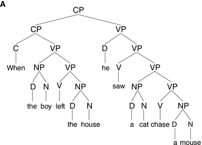
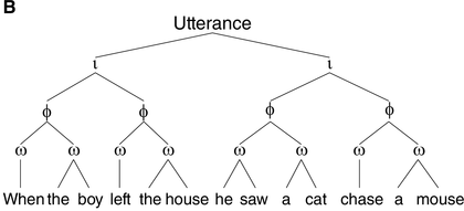
Two main paradigms have been used to study neural tracking of syntactic structure. One paradigm relies on strict control of the presentation rate of linguistic structure, whereby this structure is frequency-tagged. The idea behind this approach to tracking is that when a unit of information is repeatedly presented at a specific frequency, the neural response to that type of information becomes synchronized with its presentation rate. In a magnetoencephalography (MEG) study by Ding et al. (Reference Ding, Melloni, Zhang, Tian and Poeppel2016), participants listened to connected speech sequences of monosyllabic words, which were isochronously presented at 4 Hz (i.e., each word lasted 250 ms). Within these sequences, two adjacent words could repeatedly be grouped into 500 ms phrases, and two adjacent phrases could repeatedly be grouped into 1,000 ms sentences, such as in [S [NP new plans] [VP gave hope]]. It was found that electrophysiological brain activity concurrently tracked the time courses of words, phrases, and sentences, showing peaks in the neural power spectrum at 4 Hz (words), 2 Hz (phrases), and 1 Hz (sentences). Because all words were synthesized independently and presented isochronously, the speech sequences contained no overt prosody. As a result, only the words were clearly defined by acoustic boundaries and therefore physically discernible in the speech signal. Phrases and sentences, instead, were dissociated from prosodic cues and thus had to be internally constructed using knowledge of grammar (Burroughs et al., Reference Burroughs, Kazanina and Houghton2021; Ding et al., Reference Ding, Melloni, Zhang, Tian and Poeppel2016; Martin and Doumas, Reference Martin and Doumas2017). Indeed, neural activity emerged only at those timescales that correspond to linguistic structures: When the sequences contained words that could be grouped into two-word phrases at most, such as [NP new plans] [NP dry fur], brain recordings revealed a tracking effect at the 2 Hz phrase rate only. No effect emerged at the 1 Hz sentence rate, supposedly because there are no naturally sensible groupings present at 1 Hz. Moreover, neural tracking of syntactic structure does not appear during sleep (Makov et al., Reference Makov, Sharon and Ding2017), nor when the listener does not understand the language (Ding et al., Reference Ding, Melloni, Zhang, Tian and Poeppel2016) or when the speech is embedded in noise (Blanco-Elorrietta et al., Reference Blanco-Elorrieta, Ding, Pylkkänen and Poeppel2020), suggesting that syntactic tracking effects are linked to actual understanding (i.e., comprehension of the structures).
Because overt prosodic cues are commonly removed from the speech input in frequency-tagging studies, these effects do not easily lend themselves to a prosodic explanation. In another relevant paradigm, the same question is addressed using naturalistic stimuli in which prosody is overtly present but matched across conditions. Kaufeld et al. (Reference Kaufeld, Bosker and ten Oever2020) investigated whether neural speech tracking is modulated by the syntactic and semantic content of the linguistic input. In an electroencephalography (EEG) study, they presented participants with naturally spoken stimuli in three conditions: regular sentences, pseudoword sentences, and unstructured word lists. Tracking was quantified through phase coupling between the speech envelope and neural activity. The presentation rate of phrases, which was derived from manual annotations of the stimuli, served as the frequency band of interest (within the delta band). At this phrasal timescale, speech-brain coupling was stronger for regular sentences than for both pseudoword sentences and word lists (see also Coopmans et al., Reference Coopmans, de Hoop, Hagoort and Martin2022a). Importantly, this effect was replicated in more direct measures of syntactic tracking, that is, when coupling was computed between the EEG signal and abstract annotations that reflect syntactic structure but contain no acoustic information. These findings show that the brain tracks the timescale of syntactic phrases more strongly when this timescale contains meaningful information and is therefore relevant for language comprehension (Coopmans et al., Reference Coopmans, de Hoop, Hagoort and Martin2022a; Kaufeld et al., Reference Kaufeld, Bosker and ten Oever2020; Keitel et al., Reference Keitel, Gross and Kayser2018; ten Oever et al., Reference ten Oever, Carta, Kaufeld and Martin2022). Thus, like the tracking effects of frequency-tagging studies, these coupling-based tracking effects are linked to actual understanding of the structures.
Because these effects have been attributed to the tracking of syntactic structure (Blanco-Elorrietta et al., Reference Blanco-Elorrieta, Ding, Pylkkänen and Poeppel2020; Burroughs et al., Reference Burroughs, Kazanina and Houghton2021; Coopmans et al., Reference Coopmans, de Hoop, Hagoort and Martin2022a; Ding et al., Reference Ding, Melloni, Zhang, Tian and Poeppel2016; Kaufeld et al., Reference Kaufeld, Bosker and ten Oever2020; Martin and Doumas, Reference Martin and Doumas2017, Reference Martin and Doumas2019; ten Oever et al., Reference ten Oever, Carta, Kaufeld and Martin2022), we will conveniently refer to them as “syntactic tracking effects.” Note that this is not meant to imply that the effects are necessarily or exclusively reflective of syntactic structure. One should be skeptical of such claims of exclusivity. The brain tracks anything it recognizes, including transitional probabilities (Henin et al., Reference Henin, Turk-Browne and Friedman2021), rule-based chunks (Jin et al., Reference Jin, Lu and Ding2020), and semantic properties of words (Frank and Yang, Reference Frank and Yang2018). If these variables occur at the frequency of phrases (as they often do, even in natural language), their tracking effects will show up at the phrase rate. As already mentioned in Section 17.2, this logically means that not one of these factors exclusively explains tracking effects. Nevertheless, the idea that syntactic tracking effects can be explained in terms of prosody is quite prominent, because syntax and prosody are temporally correlated. Due to their similar periodicity, they are largely compatible with the same electrophysiological results and are therefore experimentally and analytically difficult to tease apart. In this chapter, we evaluate, both empirically and conceptually, how well prosodic explanations of syntactic tracking effects fare. In the next section (Section 17.2.2), we will discuss empirical studies linking electrophysiological signals to prosodic processing. To foreshadow our conclusion, none of these studies demonstrate purely prosodic effects. Rather, in each case we find modulatory effects of syntactic structure. This is expected given the strong relationship between syntax and prosody in natural language, which will be discussed in Section 17.3.
17.2.2 Tracking Prosodic Structure
The prosodic structure of spoken utterances is hierarchically organized. As illustrated in Figure 17.1B, an utterance contains one or more intonational phrases (denoted ι), which are composed of phonological phrases (φ, also called intermediate phrases), which are in turn composed of prosodic words (ω) (Beckman and Pierrehumbert, Reference Beckman and Pierrehumbert1986; Nespor and Vogel, Reference Nespor and Vogel1986; Selkirk, Reference Selkirk1984, Reference Selkirk, Goldschmit, Riggle and Yu2011; Shattuck-Hufnagel and Turk, Reference Shattuck-Hufnagel and Turk1996).Footnote 2 Prosodic phrasing is phonetically marked in various ways. The boundaries between ι-phrases, for instance, are cued by a silent pause, a change in pitch or fundamental frequency, and lengthening of segments preceding the boundary (Beckman and Pierrehumbert, Reference Beckman and Pierrehumbert1986; Cooper and Paccia-Cooper, Reference Cooper and Paccia-Cooper1980; Ferreira, Reference Ferreira1993; Nespor and Vogel, Reference Nespor and Vogel1986; Price et al., Reference Price, Ostendorf, Shattuck‐Hufnagel and Fong1991; Selkirk, Reference Selkirk1984; Wightman et al., Reference Wightman, Shattuck‐Hufnagel, Ostendorf and Price1992). In addition to these phonetic markers of prosodic structure, people process prosody even if it is not overtly realized in the stimulus (e.g., in reading). This is known as implicit prosody, a subvocally activated prosodic representation that is projected onto the stimulus and can affect syntactic processing in much the same way as overt prosody does (Breen, Reference Breen2014; Fodor, Reference Fodor1998, Reference Fodor2002).
Prosodic structure has rhythmic properties, with phrasal boundaries periodically occurring roughly once per second in naturally produced speech (Inbar et al., Reference Inbar, Grossman and Landau2020; Stehwien and Meyer, Reference Stehwien and Meyer2022). These low-frequency prosodic regularities provide a possible source of information for the brain to exploit. Indeed, electrophysiological studies have shown that sentential prosody is tracked by slow neural activity in the delta range. While this overlaps quite strongly with the reported timescale of syntactic processing, we will show in our discussion of these results in the current section that none of them unequivocally shows that syntactic tracking effects can be explained in terms of prosodic processing.
In spoken language comprehension, the boundaries of multi-word chunks are accompanied by a slow event-related potential (ERP) component in the EEG signal. This so-called Closure Positive Shift (CPS) is elicited by ι-boundaries that are phonetically marked through a pitch change and pre-boundary lengthening (Steinhauer et al., Reference Steinhauer, Alter and Friederici1999). Given the low-frequency rhythmicity of ι-phrases, it is expected that the neural response to repeated phrase closures has a low frequency as well. Indeed, a closure-related CPS is periodically elicited at regular two- to three-second intervals (Roll et al., Reference Roll, Lindgren, Alter and Horne2012; Schremm et al., Reference Schremm, Horne and Roll2015), and CPS effects elicited by ι-boundaries contribute to delta-band speech tracking (Inbar et al., Reference Inbar, Genzer, Perry, Grossman and Landau2023). As these CPS effects are observed even when overt prosodic cues are absent, it has been suggested that there are endogenous, time-driven constraints on the grouping of words into multi-word chunks, and that these constraints operate at a frequency corresponding to the (lower) delta band (Chapter 18; Henke and Meyer, Reference Henke and Meyer2021; Meyer et al., Reference Meyer, Henry, Gaston, Schmuck and Friederici2017; Roll et al., Reference Roll, Lindgren, Alter and Horne2012; Vetchinnikova et al., Reference Vetchinnikova, Konina, Williams, Mikušová and Mauranen2023).
In this context, it is relevant to mention a set of seemingly discrepant findings from the ERP literature. On the one hand, it has been shown in adult listeners that a CPS can be elicited by prosodically modulated stimulus sequences from which all syntactic cues are removed (e.g., hummed sentences, sentence melodies) (Gilbert et al., Reference Gilbert, Boucher and Jemel2015; Pannekamp et al., Reference Pannekamp, Toepel, Alter, Hahne and Friederici2005; Steinhauer and Friederici, Reference Steinhauer and Friederici2001). This shows that prosodic structure alone is sufficient to elicit a CPS. On the other hand, the CPS in spoken sentence processing is modulated by whether contextually induced syntactic expectations do or do not support a prosodic boundary (Kerkhofs et al., Reference Kerkhofs, Vonk, Schriefers and Chwilla2007), even to the extent that a CPS can be elicited by syntactic phrase boundaries that are not marked by prosodic boundary cues (Itzhak et al., Reference Itzhak, Pauker, Drury, Baum and Steinhauer2010). Moreover, infant studies show that prosodically induced CPS effects are dependent on syntactic development, as they are only observed in children who have acquired knowledge of phrase structure (Männel and Friederici, Reference Männel and Friederici2011). In contradiction to the earlier conclusion, these findings indicate that prosodic boundary cues are neither necessary nor sufficient to elicit a CPS. Addressing the apparent discrepancy, the results can be reconciled by the idea that, due to the tight interplay between syntax and prosody, the presence of one type of information in the input automatically activates the other. If prosodic modulations trigger syntactic representations, and syntactic cues activate prosodic structure, prosodic phrasing can be initiated even when acoustic or syntactic markers of phrase closure are not explicitly present. Either type of information is sufficient to elicit a closure-related CPS, provided that the listener is linguistically proficient – the interactive mapping between syntax and prosody requires understanding of speech structure based on syntactic knowledge (Männel and Friederici, Reference Männel and Friederici2011). Summing up this brief discussion of the ERP literature, even for a brain response that might initially seem to be a pure reflection of (implicit) prosodic processing, the role of syntax cannot be ignored.
A similar argument can be made about the results of a recent frequency-tagging study. Specifically, Glushko et al. (Reference Glushko, Poeppel and Steinhauer2022) claim that the syntactic tracking effects observed by Ding et al. (Reference Ding, Melloni, Zhang, Tian and Poeppel2016) predominantly reflect prosodic rather than syntactic processing. In Ding et al. (Reference Ding, Melloni, Zhang, Tian and Poeppel2016), the 2 Hz peak corresponded to the phrasal timescale and was therefore interpreted as reflecting syntactic tracking. The prosodic account put forward by Glushko et al. instead holds that the 2 Hz peak for sentences with a 2+2 syntactic structure, such as [NP new plans] [VP gave hope], reflects an implicit grouping of the sentence into “new plans / gave hope” (the / indicates a prosodic break), which contains two equally sized φ-phrases. This prosodic analysis is possible despite the absence of prosodic cues in isochronous speech because people are known to project implicit prosodic structure onto the input (e.g., following a same-size-sister constraint; see Section 17.3.1). In an EEG experiment, Glushko et al. (Reference Glushko, Poeppel and Steinhauer2022) used sentences with a 1+3 syntactic structure, such as [NP John] [VP likes big trees], which can be analyzed via a 2+2 prosodic grouping as well. In line with their hypothesis, these isochronously presented sentences elicit a 2 Hz peak in the neural power spectrum despite the absence of a major syntactic boundary in the middle of the sentence (i.e., between “likes” and “big”). This delta effect initially suggests that people prosodically analyzed these sentences in a way that is not suggested by their syntactic structure. However, it is not obvious that the listeners’ implicit prosodic analysis is purely prosodic, or whether it is also sensitive to the syntactic structure of the sentence. Notice that the 2+2 prosodic grouping of a sentence with such a 1+3 structure retains some of its syntactic constituency. In “John likes big trees,” for instance, the 2+2 grouping yields “John likes / big trees.” While the elements to the left of the prosodic break (“John likes”) do not form a syntactic constituent, the elements to the right of the break (“big trees”) do, making this prosodic grouping syntactically not entirely unacceptable. In other words, the prosodic units are not identical to the syntactic constituents, but the prosodic boundary does correspond to a relevant syntactic boundary. It is easy to come up with sequentially similar sentences for which this is not the case, such as [NP the cute kid] [VP laughs]. Applying a 2+2 prosodic grouping to this 3+1 structure yields “the cute / kid laughs.” This grouping intuitively sounds much less natural, plausibly because neither of the two resulting prosodic phrases corresponds to a syntactic phrase. Thus, while it initially seems that implicit groupings are induced by mechanisms other than syntactic processing, they might still be sensitive to syntax, in the sense that where people place implicit prosodic boundaries is affected by the syntactic structure underlying the sentence.
Studies with naturally produced speech also show that prosodic modulations affect low-frequency neural activity. For instance, Bourguignon et al. (Reference Bourguignon, Tiège and de Beeck2013) found similar levels of speech-brain coupling in the delta band for listeners’ native speech, nonnative speech, and hummed speech. As these effects are independent of people’s ability to process the meaning and syntactic structure of the input, they were explained in terms of the similar prosodic rhythmicity of the different stimulus types. Relatedly, Boucher et al. (Reference Boucher, Gilbert and Jemel2019) reject the idea that delta activity tracks abstract, non-sensory information. Instead, they argue that delta oscillations underlie sensory chunking via entrainment to articulated sounds. In their EEG study, participants listened to sentences, meaningless syllable strings, and tone sequences, all of which were prosodically matched by having similar patterns of timing, pitch, and energy. Delta entrainment was considerably reduced for tone sequences compared to both types of speech stimuli, arguably because tone sequences do not contain articulated sounds. No difference was found between sentences and syllable strings, suggesting that the syntactic content of sentences did not affect delta entrainment. To explain these results, Boucher et al. (Reference Boucher, Gilbert and Jemel2019) argue that delta oscillations entrain to temporal groups marked by articulated sounds, which are equally present in spoken sentences and syllable strings. This account, however, cannot explain existing work that does show a relationship between delta-band activity and the high-level linguistic content of speech. First, both Kaufeld et al. (Reference Kaufeld, Bosker and ten Oever2020) and Coopmans et al. (Reference Coopmans, de Hoop, Hagoort and Martin2022a) find stronger speech-brain coupling at the delta rate for sentences than for prosodically matched stimuli that lack syntactic structure or meaning. Second, Keitel et al. (Reference Keitel, Gross and Kayser2018) reported stronger delta-band tracking for comprehended than for uncomprehended spoken sentences. And third, recent EEG studies by Meyer et al. show that delta phase and power reflect people’s syntactic parsing choices independent of delta entrainment to speech prosody (Henke and Meyer, Reference Henke and Meyer2021; Meyer et al., Reference Meyer, Henry, Gaston, Schmuck and Friederici2017). If delta tracking only reflects the sensory chunking of speech into temporal groups, it is unclear why it is stronger for regular sentences than for prosodically matched pseudoword sentences, why it correlates with behavioral measures of comprehension, and why it is predictive of people’s syntactic analysis of a sentence.
In sum, it has been shown that delta-band neural activity tracks overt and implicit prosody during speech comprehension. Our empirical evaluation reveals both that these prosodic tracking effects are modulated by syntax and that prosodic explanations either do not cover the full range of empirical results or implicitly incorporate a notion of syntactic structure. In the rest of this chapter, we will argue that this is expected, because syntax and prosody in natural language are strongly tied together (Section 17.3). For this reason, we should not aim to explain syntactic tracking effects as being prosodic in nature, but rather, face the challenging task of determining how prosody and syntax complement and constrain one another, both in the stimulus and in the neural signal. We end by discussing such an interactive approach to syntax and prosody in the brain (Section 17.4).
17.3 The Relationship between Syntactic and Prosodic Constituency
17.3.1 Structural Alignments and Discrepancies
Prosody is often characterized in terms of the boundaries marking the edges of prosodic constituents and the relative prominence (or accent) assigned to a designated element within these constituents (Cole, Reference Cole2015; Shattuck-Hufnagel and Turk, Reference Shattuck-Hufnagel and Turk1996; Wagner and Watson, Reference Wagner and Watson2010). Both of these play an important role in language processing, but they signal different aspects of the meanings of sentences: While prosodic prominence tends to mark focus and discourse status, prosodic boundaries are commonly related to the boundaries of syntactic structure. Concerning the latter, Selkirk (Reference Selkirk1978) observed that a particular intonational contour is required for certain syntactic constituents, such as preposed adverbials (e.g., “In Pakistan // Tuesday is a holiday”), nonrestrictive relative clauses (e.g., “Tuesday // which is a weekday // is a holiday”), and parenthetical expressions (e.g., “Tuesday is // Jane said // a holiday”), each of which forms a separate ι-phrase (delineated by //). Here, the boundaries of prosodic constituents directly coincide with the boundaries marking major syntactic phrases. In most cases, however, intonational phrasing is not directly informed by syntax but rather based on prosodic structure, which is derived from syntactic constituency but not identical to it (Ferreira, Reference Ferreira1993; Féry, Reference Féry2016; Gee and Grosjean, Reference Gee and Grosjean1983; Nespor and Vogel, Reference Nespor and Vogel1986; Selkirk, Reference Selkirk1984).
Recall that segments at the end of prosodic phrases are often lengthened and followed by a pause (Cooper and Paccia-Cooper, Reference Cooper and Paccia-Cooper1980; Ferreira, Reference Ferreira1993; Nespor and Vogel, Reference Nespor and Vogel1986; Price et al., Reference Price, Ostendorf, Shattuck‐Hufnagel and Fong1991; Wightman et al., Reference Wightman, Shattuck‐Hufnagel, Ostendorf and Price1992). Structurally ambiguous phrases, such as “old men and women,” can be disambiguated by these prosodic cues. That is, the word “men” and the subsequent pause are longer in “old men / and women,” where they occur at the end of a noun phrase, than in “old / men and women,” where they occur phrase-medially. As prosodic phrase boundaries tend to align with syntactic phrase boundaries, acoustic cues such as pre-boundary lengthening provide information about syntactic structure. However, these cues are not diagnostic, because pre-boundary lengthening can vary in the absence of syntactic differences. For instance, compared to longer subjects, shorter subjects are less likely to be accompanied by boundary-related phonetic cues in production (pre-boundary lengthening and subsequent pause; Gee and Grosjean, Reference Gee and Grosjean1983; Watson and Gibson, Reference Watson and Gibson2004) and they do not elicit a CPS in comprehension (Hwang and Steinhauer, Reference Hwang and Steinhauer2011). Rather than directly reflecting syntax, it appears that the magnitude of pre-boundary lengthening effects is related to the perceived strength of prosodic boundaries (Ferreira, Reference Ferreira1993; Price et al., Reference Price, Ostendorf, Shattuck‐Hufnagel and Fong1991; Wightman et al., Reference Wightman, Shattuck‐Hufnagel, Ostendorf and Price1992). Thus, syntactic structure affects phonetic variation indirectly, through intermediate prosodic structure.
It has repeatedly been observed that prosodic structure reflects syntactic structure in important ways, but is not isomorphic to it (Ferreira, Reference Ferreira1993; Féry, Reference Féry2016; Gee and Grosjean, Reference Gee and Grosjean1983; Nespor and Vogel, Reference Nespor and Vogel1986; Selkirk, Reference Selkirk1984). Several arguments have been presented for a prosodic structure representation that is distinct from syntactic structure (Selkirk, Reference Selkirk, Goldschmit, Riggle and Yu2011; Shattuck-Hufnagel and Turk, Reference Shattuck-Hufnagel and Turk1996). First, the two have different formal properties. Compared to syntactic hierarchies, which are deeply embedded and fundamentally asymmetrical, prosodic structure is symmetrical and rather flat (Gee and Grosjean, Reference Gee and Grosjean1983; Nespor and Vogel, Reference Nespor and Vogel1986; Selkirk, Reference Selkirk1978, Reference Selkirk1984). Second, prosodic constituents may systematically deviate from syntactic constituents. For instance, the sentences “John is eager to please” and “John is easy to please” are superficially similar and, when produced naturally, receive the same analysis in terms of prosodic constituency. However, their underlying syntactic structures are very different: “John” is the subject of “please” in the first sentence, but its object in the second sentence. Moreover, prosodically well-formed sequences may be syntactically unacceptable, as in the ungrammatical “John is easy to please Mary.” Note again that the prosodically similar “John is eager to please Mary” is fully acceptable, showing that syntactic deviance need not be reflected in prosodic deviance. Third, and conversely, there is considerable variability in the prosodic realization of one and the same syntactic structure. Non-syntactic factors such as speech rate, semantic coherence, discourse status, and independent phonological well-formedness constraints all affect prosodic structuring (Ferreira, Reference Ferreira1993; Frazier et al., Reference Frazier, Clifton and Carlson2004; Gee and Grosjean, Reference Gee and Grosjean1983; Nespor and Vogel, Reference Nespor and Vogel1986; Selkirk, Reference Selkirk1984, Reference Selkirk, Goldschmit, Riggle and Yu2011; Watson and Gibson, Reference Watson and Gibson2004).
One such non-syntactic factor that has received considerable attention is the same-size-sister constraint, which reflects speakers’ tendency to place boundaries at locations such that the prosodic phrases on both sides of the boundary are roughly the same weight and length (Cooper and Paccia-Cooper, Reference Cooper and Paccia-Cooper1980; Fodor, Reference Fodor1998; Gee and Grosjean, Reference Gee and Grosjean1983). This preference for balance results in symmetry in the prosodic hierarchy (see Figure 17.1B), contrasting with the asymmetrical structure of syntactic hierarchy (Figure 17.1A). A well-known case is presented by recursively embedded clauses, such as “this is the cat that chased the rat that ate the cheese.” The syntactic structure of this sentence is asymmetrical and deeply nested, as shown by the number of closing brackets at the end of [this [is [the cat [that chased [the rat [that ate [the cheese]]]]]]]. When produced naturally, however, the intonational bracketing is rather flat, roughly corresponding to “this is the cat // that chased the rat // that ate the cheese,” with all ι-phrases being approximately the same size, and with none of the ι-breaks corresponding to clause boundaries (Chomsky and Halle, Reference Chomsky and Halle1968). That prosodic boundaries might occur at places that are not major syntactic boundaries is also seen in Figure 17.1B, where the subject and the finite verb in the main clause form a prosodic constituent (the ω-word “he saw”) to the exclusion of the object (“a cat chase a mouse”), which is not consistent with the syntactic constituency analysis (Figure 17.1A).
To sum up, syntax and prosody are systematically related, but their structures are not isomorphic. According to Féry (Reference Féry2016), the relation of syntax to prosody is one of homomorphism. Homomorphic maps are structure-preserving, but in contrast to isomorphisms they need not be one to one, which means that the inverse relation is not necessarily structure-preserving. In other words, the structure of syntax is preserved in prosodic structure, but because of the smaller number of constituents in the prosodic structure, not all syntactic details are retained in the map.Footnote 3 Syntactic structure therefore cannot uniquely be derived from prosodic patterns. This would explain why prosodic boundaries nearly always index syntactic boundaries, while many syntactic boundaries are not prosodically marked.
17.3.2 Syntax–Prosody Interactions in Language Processing
Given that the boundaries of prosodic structure tend to align with syntactic phrase boundaries, prosodic information can be used as an informative cue during syntactic processing, and conversely, knowledge of syntax can be used to make inferences about prosodic structure (for reviews, see Cutler et al., Reference Cutler, Dahan and Van Donselaar1997; Wagner and Watson, Reference Wagner and Watson2010). Concerning the former, behavioral studies with syntactically ambiguous sentences show that people use prosodic boundary cues to resolve temporary syntactic ambiguities in comprehension and production (Kjelgaard and Speer, Reference Kjelgaard and Speer1999; Marslen-Wilson et al., Reference Marslen-Wilson, Tyler, Warren, Grenier and Lee1992; Millotte et al., Reference Millotte, Wales and Christophe2007; Schafer et al., Reference Schafer, Speer, Warren and White2000; Speer et al., Reference Speer, Kjelgaard and Dobroth1996). For instance, in a constrained production experiment by Schafer et al. (Reference Schafer, Speer, Warren and White2000), participants had to produce sentences with early- versus late-closure ambiguities, as in the examples below. In the late-closure analysis of the subordinate clause, “the square” is the direct object of “moves” (as in 2), whereas it is the subject of the main clause when the subordinate clause is closed early (as in 1). Speakers consistently placed an ι-boundary at the subordinate clause boundary, whose location varied depending on the meaning the speakers wanted to convey.
1. When that triangle moves // the square will …
2. When that triangle moves the square // it …
In a subsequent comprehension experiment, it was found that listeners use the speakers’ prosodic phrasing to constrain their syntactic analysis (Schafer et al., Reference Schafer, Speer, Warren and White2000). The same results are reported for globally ambiguous sentences, which show that speakers and listeners typically avoid attaching two syntactic constituents that are separated by a prosodic break. In a sentence such as “when you learn gradually you worry more,” people use prosodic boundaries to disambiguate the intended reading (here, left versus right attachment of “gradually”), both in speaking and in listening (Kraljic and Brennan, Reference Kraljic and Brennan2005; Price et al., Reference Price, Ostendorf, Shattuck‐Hufnagel and Fong1991; Snedeker and Trueswell, Reference Snedeker and Trueswell2003).
Similar effects of prosodic phrasing on the interpretation of locally ambiguous sentences are reported in the ERP literature. These effects reflect not only the processing of the prosodic boundary itself (see Section 17.2.2) but also its downstream consequences for sentence interpretation. Consider the sentences in 3 and 4, which are identical up to the embedded verb (Bögels et al., Reference Bögels, Schriefers, Vonk, Chwilla and Kerkhofs2010). Depending on the argument structure of this verb, de soldaat “the soldier” is either the object in the embedded sentence (in 4, when the embedded verb is the transitive vermoorden “to kill”) or the direct object of the main verb beval “ordered” (in 3, when the embedded verb is the intransitive vuren “to fire”). If the sentence is presented without overt prosodic boundaries and is truncated before the embedded verb, people have a preference for the intransitive reading.
3. De commandant beval // de soldaat te vuren en …
The commander ordered // the soldier to fire and …
4. De commandant beval // de soldaat te vermoorden en …
The commander ordered // to kill the soldier and …
When these sentences are presented with the intonational phrasing indicated, the ι-boundary after the verb beval “ordered” elicits a CPS in the ERP signal, indexing the closure of a prosodic phrase. Moreover, because people are biased against integrating information across a prosodic boundary, the presence of this ι-boundary creates the expectation that the upcoming words will form a constituent. This means that de soldaat “the soldier” is initially not interpreted as belonging to beval “ordered,” but rather as the object of the upcoming verb, which is therefore expected to be transitive (as in 4). Indeed, the disambiguating intransitive verb in 3 elicited an increased N400, reflecting processing difficulty associated with a verb whose argument structure violates a prosody-induced syntactic expectation (Bögels et al., Reference Bögels, Schriefers, Vonk, Chwilla and Kerkhofs2010; Friederici et al., Reference Friederici, von Cramon and Kotz2007; Steinhauer et al., Reference Steinhauer, Alter and Friederici1999). Corroborating the behavioral data, these ERP results show that prosodic information can determine people’s syntactic analyses of locally ambiguous sentences by completely reversing their default parsing preferences (see also Henke and Meyer, Reference Henke and Meyer2021).
It is important to note that prosody can only disambiguate two interpretations of the same sentence if their constituent boundaries are located at different places (Nespor and Vogel, Reference Nespor and Vogel1986). An ambiguous sentence such as “flying planes can be dangerous” is difficult to disambiguate prosodically because the words that cause the ambiguity – “flying planes” – form a syntactic constituent in both meanings. Even for structurally ambiguous sentences, however, a local prosodic boundary is not an unambiguous cue to syntactic closure or attachment. Rather, what matters is the global prosodic representation, in which the informativeness of a prosodic boundary is evaluated relative to other prosodic and phonological cues, including the strength of other boundaries and the lengths of the constituents it flanks. That is, a φ-boundary is more decisive syntactically when it is the only prosodic cue than when it is preceded by a phonologically stronger ι-boundary (Carlson et al., Reference Carlson, Clifton and Frazier2001; Clifton et al., Reference Clifton, Carlson and Frazier2002). And prosodic boundaries are perceived to be more informative about the intended structure of a sentence when they flank short constituents than when they flank long constituents (Clifton et al., Reference Clifton, Carlson and Frazier2006). Other things being equal, the probability of a prosodic boundary increases when the constituents surrounding it are longer (Ferreira, Reference Ferreira1993; Frazier et al., Reference Frazier, Clifton and Carlson2004; Gee and Grosjean, Reference Gee and Grosjean1983; Hwang and Steinhauer, Reference Hwang and Steinhauer2011; Watson and Gibson, Reference Watson and Gibson2004). Thus, when the surrounding constituents are short, the prosodic boundary is not justified by constituent length, so listeners assume it to be driven by syntactic structure (Clifton et al., Reference Clifton, Carlson and Frazier2006). In accordance with the non-isomorphism between prosodic and syntactic structure, prosodic phrasing cues syntactic decomposition probabilistically, not diagnostically.
Concerning the effect of syntax on prosodic parsing, it has been shown that syntactic constituency guides the perception of prosody. Cole et al. (Reference Cole, Mo and Baek2010) asked untrained listeners to prosodically transcribe naturalistic speech and found that syntactic context made an independent contribution to the perception of prosodic boundaries. Similarly, in a prosodic boundary detection task with spoken sentences, Buxó-Lugo and Watson (Reference Buxó-Lugo and Watson2016) found that the probability of boundary marking was higher for syntactically licensed locations than for non-licensed locations, even when the acoustic properties of the boundaries were experimentally controlled (see also Fodor and Bever, Reference Fodor and Bever1965). These two studies show that prosodic boundaries are perceptually more salient when they coincide with the boundaries of syntactic constituents. This is in line with acquisition studies showing that children are sensitive to the acoustic correlates of syntactic structure. Very young infants prefer speech in which artificially inserted pauses coincide with syntactic phrase boundaries compared to speech in which the pauses are inserted in the middle of phrases (Hirsh-Pasek et al., Reference Hirsh-Pasek, Kemler Nelson and Jusczyk1987; Jusczyk et al., Reference Jusczyk, Hirsh-Pasek and Kemler Nelson1992; Kemler Nelson et al., Reference Kemler Nelson, Hirsh-Pasek, Jusczyk and Cassidy1989). What is more, infants use their sensitivity to the prosodic marking of syntactic units to recognize these units in natural speech. After being familiarized with phonological word sequences that were spoken both as a prosodically well-formed syntactic constituent and as a syntactic non-constituent (i.e., the prosodic structuring indexed syntactic constituency), infants prefer listening to passages in which the sequences constitute a constituent over passages in which the sequences cross a phrase boundary and form a non-constituent (Soderstrom et al., Reference Soderstrom, Seidl, Kemler Nelson and Jusczyk2003). Prosodic well-formedness thus facilitates the identification and recognition of syntactic units in continuous speech.
There might be a role for delta tracking in modulating this relationship between syntactic and prosodic grouping. Infants’ preference for coinciding syntactic and prosodic boundaries holds more strongly for child-directed speech than for adult-directed speech (Kemler Nelson et al., Reference Kemler Nelson, Hirsh-Pasek, Jusczyk and Cassidy1989). A possible reason is that child-directed speech is characterized by strong delta-band regularities (i.e., enhanced amplitude modulation and rhythmic regularity; Leong et al., Reference Leong, Kalashnikova, Burnham and Goswami2017), which support the perceptual inference of higher-level linguistic structure. Indeed, it has been observed in young infants that speech-brain coupling at the prosodic stress rate is higher for child-directed speech than for adult-directed speech (Menn et al., Reference Menn, Michel, Meyer, Hoehl and Männel2022). Given that prosodic boundaries often coincide with syntactic boundaries, the infant brain might be able to bootstrap its syntactic acquisition by neurally tracking the prosodic delta-band modulations that are prominent in child-directed speech (Jusczyk et al., Reference Jusczyk, Hirsh-Pasek and Kemler Nelson1992; Männel and Friederici, Reference Männel and Friederici2011; Soderstrom et al., Reference Soderstrom, Seidl, Kemler Nelson and Jusczyk2003).
17.4 Integrating Prosodic and Syntactic Accounts of Neural Tracking Effects
In the preceding sections, we have given several reasons for why we should not attempt to explain syntactic tracking effects in prosodic terms (or vice versa). Our arguments are logical (i.e., due to the absence of one-to-one mappings, neural signals do not uniquely index cognitive events; see Section 17.2), empirical (i.e., the neural correlates of prosodic processing are modulated by syntax; see Section 17.2.2), and ontological (i.e., prosodic and syntactic constituency are ontologically related; see Section 17.3). In this last section, we will offer a fourth argument, which is more strategic. That is, because neither prosody nor syntax ever appears in isolation in natural language, it makes sense if neurobiological investigations of language attempt to determine how the interaction between prosody and syntax, both in the stimulus and in the brain, facilitates processing. This aligns naturally with what we perceive to be the goal of the neurobiology of language, that is, to explain how the interplay between different sources of linguistic information ultimately yields comprehension via neurobiological mechanisms.
By presenting this strategic argument in favor of an integrative approach, we do not mean to say that a disjunctive approach, in which it is investigated whether and to what extent single cognitive factors modulate neural processing, should not be pursued. On the contrary, this approach is required to determine whether the brain cares about a given cognitive feature in the first place, so it naturally precedes the integrative approach. However, when its results are interpreted, it is important to keep in mind that in natural language processing, the brain never encounters that feature in isolation. It should therefore be acknowledged that single-component explanations are only part of the story, and that a conjunctive understanding is ultimately desired. Moreover, when researchers try to isolate the contribution of one factor (e.g., prosody, syntax) as part of the disjunctive approach, it is important that they take adequate caution in their experimental designs by establishing proper baselines for neural responses that are amenable to a high-level linguistic explanation. This is particularly important when one aims to dissociate the neural contributions of two factors that are highly correlated. It can be done by including control conditions that only differ from the experimental condition in the variable of interest (e.g., natural sentences versus prosodically matched pseudoword sentences; Coopmans et al., Reference Coopmans, de Hoop, Hagoort and Martin2022a; Kaufeld et al., Reference Kaufeld, Bosker and ten Oever2020), or by including prosodic control predictors in encoding models of language-related brain activity (Slaats et al., Reference Slaats, Weissbart, Schoffelen, Meyer and Martin2023). Properly accounting for prosodic variance will be helpful in detecting and understanding the remaining effects whose variance in neural dynamics is more directly attributable to syntactic processing (i.e., “true” syntactic tracking effects).
In line with this disjunctive approach, many recent studies have tried to dissociate different linguistic factors in order to account for the linguistic properties underlying tracking effects. This approach has been very effective and successful, but such functional decompositions are not the end result when the ultimate aim is to explain how language is represented in the brain. While syntax and prosody comprise formally distinct systems (Beckman and Pierrehumbert, Reference Beckman and Pierrehumbert1986; Féry, Reference Féry2016; Ferreira, Reference Ferreira1993; Nespor and Vogel, Reference Nespor and Vogel1986; Selkirk, Reference Selkirk1978, Reference Selkirk1984, Reference Selkirk, Goldschmit, Riggle and Yu2011; Shattuck-Hufnagel and Turk, Reference Shattuck-Hufnagel and Turk1996), it is unlikely that the brain strictly distinguishes them during natural language comprehension, precisely because they are so strongly tied together. Thus, beyond trying to attribute tracking effects exclusively to one linguistic component, or looking at the remaining variance to be explained by that one component, we consider it critical to also think about ways in which the interaction between the components (linguistic or otherwise) drives the neural signal. When it comes to syntax and prosody, this type of interactive approach is common both in theoretical linguistics (e.g., Féry, Reference Féry2016; Nespor and Vogel, Reference Nespor and Vogel1986; Selkirk, Reference Selkirk1984, Reference Selkirk, Goldschmit, Riggle and Yu2011) and psycholinguistics (e.g., Bögels et al., Reference Bögels, Schriefers, Vonk, Chwilla and Kerkhofs2010; Buxó-Lugo and Watson, Reference Buxó-Lugo and Watson2016; Coopmans et al., Reference Coopmans, Struiksma, Coopmans and Chen2022b; Friederici et al., Reference Friederici, von Cramon and Kotz2007; Hwang and Steinhauer, Reference Hwang and Steinhauer2011; Itzhak et al., Reference Itzhak, Pauker, Drury, Baum and Steinhauer2010; Kerkhofs et al., Reference Kerkhofs, Vonk, Schriefers and Chwilla2007; Kjelgaard and Speer, Reference Kjelgaard and Speer1999; Steinhauer et al., Reference Steinhauer, Alter and Friederici1999), but the literature on neural speech tracking remains predominantly focused on single-component explanations.
With the advanced analysis techniques that have become available in recent years, it is now possible to study the neural basis of language comprehension in naturalistic contexts (e.g., audiobook listening), where the interaction between, and co-occurrence of, syntactic and prosodic information is natural and commonplace. In a recent MEG decoding study, Degano et al. (Reference Degano, Donhauser, Gwilliams, Merlo and Golestani2023) utilized this opportunity and found that the neural encoding of syntactic information in natural speech is boosted by prosody. This important result indicates that the alignment between syntax and prosody yields a syntactic representational gain in the neural signal (Degano et al., Reference Degano, Donhauser, Gwilliams, Merlo and Golestani2023), and more generally, it shows the promise of the interactive approach. The time is ripe for cognitive neuroscientists to investigate how the brain interprets and constructs spoken language by (de)composing the mutually constraining rhythms of syntactic and prosodic structures. But while doing so, it is important to keep in mind that neural tracking of a given variable, be it physical or linguistic, may only be the tip of the iceberg in terms of the infrastructure for language comprehension in the brain.
17.5 Funding Information
Andrea E. Martin was supported by an Independent Max Planck Research Group and a Lise Meitner Research Group “Language and Computation in Neural Systems,” by NWO Vidi grant 016.Vidi.188.029 to AEM, and by Big Question 5 (to Prof. dr. Roshan Cools and Dr. Andrea E. Martin) of the Language in Interaction Consortium funded by NWO Gravitation Grant 024.001.006 to Prof. dr. Peter Hagoort. Cas W. Coopmans was supported by NWO Vidi grant 016.Vidi.188.029 to AEM.
17.6 Acknowledgements
We are grateful to Hatice Zora and two anonymous reviewers for valuable comments on an earlier draft of this chapter.
Summary
Empirical results in the literature on neural speech tracking are commonly attributed to either syntax or prosody. Here, we present four types of arguments against attempts to explain putatively syntactic tracking effects in prosodic terms (or vice versa). The arguments are based on logic, empirical observations, ontology, and strategy.
Implications
Because syntactic and prosodic structure are strongly related in speech and language, future research should be less focused on disjunctive explanations of neural tracking effects. Instead, researchers should attempt to explain how the natural interaction between syntactic and prosodic information, and their functional interdependence, drives the neural signal.
Gains
The interrelatedness between syntax and prosody is well known in linguistics, and their interactions have been widely studied in psycholinguistics. We show that when this interactive approach is embraced in cognitive neuroscience as well, it will greatly increase our understanding of how the brain makes sense of natural language.
18.1 Introduction
Language comprehension is guided by external acoustic cues but may also have an internal, implicit realization, influencing processing from the inside out – that is, endogenously. In particular, there are a number of endogenous constraints that influence the timing and pace of language processing. Some of these constraints may reflect cognitive and neural processing limitations, such as properties of working memory or even the electrophysiology of the brain as such. These context-invariant endogenous constraints interact with the current context of linguistic representations that are built during incremental language processing.
In this chapter, we first review behavioural evidence from psycholinguistics, describing the complex interaction of syntactic, prosodic, and information structures during the integration of words into larger multi-word units across substantial temporal intervals. In the second part, we summarize evidence from event-related brain potentials (ERPs) supporting the idea that temporal processing windows in the order of multiple seconds shape language production and comprehension endogenously. Lastly, we suggest that the repetitive pace of these integration windows may trigger a certain extent of rhythmicity in language behaviour. We discuss recent evidence that temporal electrophysiological constraints are driven by underlying endogenous oscillatory activity that acts as a pacemaker on language processing.
18.2 Timing Constraints on Linguistic Processing in Behaviour
The timing of linguistic processing is driven by the incremental computation of linguistic representations, including prosodic, syntactic, and information structures. As language comprehension unfolds over time, the online computation of these structures (e.g., “where” to place a boundary within a syntactic tree) may be influenced by contextual temporal constraints (e.g., “when” to expect a syntactic boundary given the preceding acoustic and abstract context). Here, we first focus on the temporal relationship between (implicit) prosody and syntax, and how they relate to the context-invariant constraints of working memory capacity. We then describe how syntax and prosody further interact with information structure to place contextual constraints on the timing of language processing.
There is a close relationship between syntactic and prosodic structure (for reviews, see Dahan, Reference Dahan2015; Dahan and Ferreira, Reference Dahan, Ferreira and Hagoort2019; for further discussion of the prosody–syntax interface and its interaction with informativity, see Chapter 19). While not strictly one to one, syntactic phrase boundaries often co-occur with prosodic boundaries in spoken language (Clifton et al., Reference Clifton, Carlson and Frazier2002; Ferreira, Reference Ferreira1993; Selkirk, Reference Selkirk, Goldsmith, Riggle and Yu2011). Thus, prosody is an important cue to syntax: Listeners rely on the perception of prosodic boundaries to infer syntactic structure, particularly in cases of syntactic ambiguity. For example, in the sentence The friend of the moviestar who was sitting on the balcony was under investigation, the relative clause (who was sitting on the balcony) can either be attached “high” in the syntactic tree (to the first noun, the friend) or “low” (to the second noun, the moviestar; see Figure 18.1). During incremental processing of the sentence, comprehenders must choose what the relative clause attaches to, thus arriving at different semantic interpretations of the sentence (whether it was the friend or the moviestar that was on the balcony). Studies suggest that this syntactic choice depends on cross-linguistic attachment preferences (e.g., a preference for low attachment in English, as opposed to high attachment in Spanish; Carreiras and Clifton, Reference Carreiras and Clifton1999) as well as constraints in working memory capacity, further discussed below (Swets et al., Reference Swets, Desmet, Hambrick and Ferreira2007; Traxler, Reference Traxler2009). Importantly, prosodic boundaries following either the first or second noun have been shown to influence syntactic attachment choices, generally leading to more high attachment when the boundary follows the second noun (Carlson et al., Reference Carlson, Clifton and Frazier2001; Clifton et al., Reference Clifton, Carlson and Frazier2002; Frazier et al., Reference Frazier, Carlson and Clifton2006).Footnote 1 However, syntactic choices are not simply driven by the presence or absence of a prosodic boundary or its acoustic realization (e.g., the absolute duration of a pause or pitch height of a boundary tone) but rather by the global prosodic structure over the entire sentence (e.g., the duration of a prosodic pause or height of a boundary tone relative to previous pauses and intonation patterns; Clifton et al., Reference Clifton, Carlson and Frazier2002). This suggests that during spoken language comprehension, listeners incrementally build a representation of a prosodic structureFootnote 2, which then influences the computation of a syntactic structure (parsing) by constraining the temporal location of syntactic boundaries. Thus, it is the relationship between the acoustic characteristics of prosodic boundaries over a long time window (the entire sentence), rather than the individual duration and pitch of each boundary, that is thought to play a critical role in syntactic processing.
Relative clause attachment ambiguities.
Illustration of the attachment ambiguity highlighting the two possible attachment sites for the relative clause. The relative clause may be attached high in the syntactic tree (bold) combining it with the friend
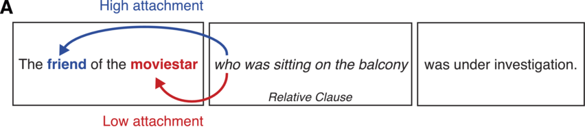
when there is a (implicit) prosodic boundary after the moviestar. Alternatively, it may be attached low in the syntactic tree (bold) such that it is the moviestar who was sitting on the balcony
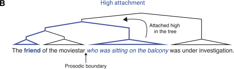
when the boundary only occurs later in the sentence.
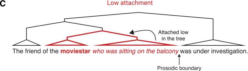
The influence of prosodic constraints on syntactic parsing is not limited to spoken language. Even in silent reading, comprehenders appear to make syntactic decisions based on an internal, implicit realization of prosodic structure (Fodor, Reference Fodor2002). For example, Swets et al. (Reference Swets, Desmet, Hambrick and Ferreira2007) appeal to the concept of implicit prosody in order to explain their findings on the relationship between syntactic attachment preferences and working memory capacity. It was previously suggested that in cases of syntactic attachment ambiguities (as in the example above), comprehenders with low working memory span prefer low attachment, since the second noun is more recent and accessible than the first noun, which would need to be retrieved from working memory (the recency principle or late closure; Frazier, Reference Frazier1979; Traxler, Reference Traxler2007). However, Swets et al. found the opposite pattern: Readers with low working memory span were more likely to attach high compared to readers with high spans. In a following study, they tested whether implicit prosody mediates this chunking strategy. Readers with high spans may tend to chunk a larger amount of information together, combining the second noun with the relative clause in a single prosodic phrase; on the other hand, readers with low spans may chunk less information together, adding an implicit prosodic boundary between the second noun and the start of the relative clause. These two prosodic patterns would be consistent with a preference to attach low or high, respectively (see Figure 18.1B, C). Swets et al. (Reference Swets, Desmet, Hambrick and Ferreira2007) provide evidence for this interpretation by presenting their sentences in chunks, forcing all readers to insert a boundary following the second noun, resulting in high attachment regardless of readers’ working memory span. Later similar findings support this idea (Hemforth et al., Reference Hemforth, Fernandez and Clifton2015; Jun and Bishop, Reference Jun and Bishop2015; Traxler, Reference Traxler2009), and a large literature suggests that silent reading involves the computation of an implicit prosodic structure (for a review, see Breen, Reference Breen2014). Thus, even in the absence of overt articulation, comprehenders are thought to compute an internal prosodic structure constrained by context-invariant individual differences in working memory capacity. In particular, working memory capacity may determine the amount of chunked information and therefore the duration of prosodic phrases.
While Swets et al.’s findings contradict initial assumptions about the role of working memory in syntactic ambiguity resolution, they support an indirect effect of individual differences in working memory capacity mediated by prosodic phrasing. This effect is consistent with the early “sausage-machine” model of parsing (Frazier and Fodor, Reference Frazier and Fodor1978), which argues that syntactic parsing occurs over two stages: an initial stage that groups words into chunks of limited size (the Preliminary Phrase Packager), and a secondary stage that builds a full syntactic analysis based on these chunks (the Sentence Structure Supervisor). In this model, the size of the initial chunks was posited to be limited to approximately six words by working memory limitations; it follows that individual differences in working memory capacity would lead to differences in the size of these initial chunks.Footnote 3 In their discussion, Swets et al. (Reference Swets, Desmet, Hambrick and Ferreira2007) speculate that the size of the chunks produced through this first stage of parsing (constrained by working memory) may be responsible for the introduction of implicit prosodic boundaries and, subsequently, syntactic attachment choices. We further elaborate on the context-invariant constraint of working memory capacity on the size and duration of syntactic phrases in the next sections.
One additional contextual constraint placed by prosody and syntax relates to their interaction with another important aspect of language: information structure. Information structure is a term from linguistic pragmatics that describes how sentences organize given information (= what the listener already knows) and new information (= what the listener does not know yet), within the context of a broader discourse or conversation. In many languages, sentences often present given information first and new information last. This given-before-new strategy reflects greater accessibility of given information during production, and is thought to facilitate comprehension by helping the listener retrieve concepts from long-term memory before appending new information (Bock and Irwin, Reference Bock and Irwin1980; Christianson and Ferreira, Reference Christianson and Ferreira2005; Ferreira and Yoshita, Reference Ferreira and Yoshita2003; Haviland and Clark, Reference Haviland and Clark1974). However, speakers can deviate from this default information structure, cueing listeners towards focused, important information through prosodic prominence (e.g., JOHN ate the sandwich) or the use of specific syntactic structures (e.g., It was John who ate the sandwich; Carlson et al., Reference Carlson, Dickey, Frazier and Clifton2009; but see Vallduví, Reference Vallduví, Aloni and Dekker2016, for debates on terminology). There are cross-linguistic differences in whether speakers focus important information primarily prosodically (e.g., English and Dutch; Breen et al., Reference Breen, Fedorenko, Wagner and Gibson2010; Nooteboom and Kruyt, Reference Nooteboom and Kruyt1987) or syntactically (e.g., Spanish and Italian; Samek-Lodovici, Reference Samek-Lodovici2005; Zubizarreta, Reference Zubizarreta1998), also leading listeners to differently weigh each of these focus cues to infer information structure across languages (Calhoun et al., Reference Calhoun, Wollum and Kruse Va’ai2021; Kember et al., Reference Kember, Choi, Yu and Cutler2019; Yan and Calhoun, Reference Yan and Calhoun2020).
Inferring the upcoming information structure of a sentence as it unfolds places temporal constraints on all levels of language processing. Listeners are thought to predict the timing of important information so that attention and processing resources can be pre-allocated to it (Beier and Ferreira, Reference Beier, Ferreira, Cutler and Fodor2022; Cutler and Fodor, Reference Cutler and Fodor1979; Kristensen et al., Reference Kristensen, Wang, Petersson and Hagoort2013). In addition, information structure has been shown to interact with other key aspects of language comprehension, including semantic (Wang et al., Reference Wang, Hagoort and Yang2009, Reference Wang, Bastiaansen, Yang and Hagoort2011) and syntactic processing (Wang et al., Reference Wang, Bastiaansen, Yang and Hagoort2012). Focused words are read for longer (Lowder and Gordon, Reference Lowder and Gordon2015) and are remembered better (Birch and Garnsey, Reference Birch and Garnsey1995), while comprehenders may be more likely to engage in “good-enough” processing for already given information (Ferreira and Lowder, Reference Ferreira and Lowder2016). However, more research is needed to establish how listeners use syntactic and prosodic focus cues to incrementally infer upcoming information structure and how this interacts with language comprehension over time.
In summary, as language unfolds over time, processing is constrained by the incremental computation of syntactic, prosodic, and information structures and the temporal relationship between them. During spoken language comprehension, acoustic features are weighed to infer a sentence’s prosodic structure, which then guides syntactic choices. This occurs even in silent reading, where context-invariant individual differences in working memory capacity constrain the duration of (implicit) prosodic and syntactic phrases. Prosody and syntax further serve as cues to upcoming information structure, guiding the comprehender’s attention towards the timing of important information and interacting with all levels of linguistic processing.
18.3 Time-Limited Integration Windows: Evidence from ERPs
In the previous section, we discussed early psycholinguistic work that suggested that phrases or constituents are constrained to a length of around six words (Frazier and Fodor, Reference Frazier and Fodor1978). However, this constraint may not reflect a limitation in the number of words but rather a temporal constraint that limits the duration of linguistic structures within our processing capacity. For instance, studies of prosodic phrasing provide evidence that the duration of phrases plays an important role in the determination of boundaries (for a detailed discussion on prosodic phrasing as a cue for cognitive dynamics, see Chapter 15). Accordingly, prolonged phrase durations lead to a different overt prosodic phrasing and increase the likelihood for implicit prosodic boundaries (Hirose, Reference Hirose2003; Hwang and Schafer, Reference Hwang and Schafer2009; Webman-Shafran and Fodor, Reference Webman-Shafran and Fodor2016). Hence, temporal windows may shape the formal side of language production and perception.
The proposed six-word limit – assuming an average speech rate of approximately 150 words per minute (Tauroza and Allison, Reference Tauroza and Allison1990) – results in multi-word units of about 2.4 seconds. Likewise, speech production data suggests that spoken language tends to be delivered in chunks of around 2.6 seconds (Vollrath et al., Reference Vollrath, Kazenwadel and Krüger1992). Notably, this slow time constant corresponds to the maximum duration of word forms held in working memory. Baddeley et al. (Reference Baddeley, Thomson and Buchanan1975) argued that phonological working memory traces decay after 2–3 seconds. Sachs (Reference Sachs1967, Reference Sachs1974) found that after more than 3 seconds of intervening speech, listeners had great difficulties identifying form-related (grammatical) but not semantic changes. She proposed that the form and syntactic details of sentences are clear and accessible in working memory for only a few seconds. During that short time window, however, the conveyed message is recoded into a more durable semantic representation.
Roll et al. (Reference Roll, Lindgren, Alter and Horne2012) hypothesized that intonational phrases tend to be uttered within time windows of 2–3 seconds to be parseable while the word forms are still active in working memory. A more specific time constant was obtained by letting speakers read sentences that could be phrased in different ways. Speakers increased their speech rate for longer phrases, seemingly trying to fit them within a time window of 2.7 seconds. This duration was taken as the ideal duration of intonational phrases. To determine whether prosodic phrasing automatically proceeds in windows of 2.7 seconds during perception while controlling for acoustic factors, silent reading has been investigated using ERPs. In auditory processing, intonational phrase boundaries yield a positive-going shift in listeners’ ERPs called the closure positive shift (CPS; Steinhauer et al., Reference Steinhauer, Alter and Friederici1999). A CPS has even been found in silent reading at commas, where readers close phrase boundaries (Steinhauer and Friederici, Reference Steinhauer and Friederici2001). Roll et al. (Reference Roll, Lindgren, Alter and Horne2012) presented participants with sentences word by word to see if they would spontaneously integrate or chunk them into 2.7-second phrases. Sentences could be chunked in three different possible phrasings. Phrases could correspond to one, two, or three clauses. The sentence material was presented at different rates so that either one, two, or all three clauses of each sentence would fall within a time window of 2.7 seconds. In this way, a CPS was observed whenever a possible phrase boundary corresponded to a 2.7-second duration from a clause onset (see Figure 18.2). Due to the varying presentation rate, the phrase endings that elicited a CPS thus contained one, two, or three clauses. An additional control condition with an extra word in each clause allowed the researchers to investigate what happened when clauses exceeded the 2.7-second time window. For these 3.4-second-long clauses, there was a difference for participants with high and low working memory spans. Whereas the high-span group showed no difference between longer and shorter clauses, the low-span group exhibited a left parietal negativity for the longer compared to the shorter clauses, suggesting that stimuli exceeding the common time window were more taxing on working memory.
Presentation rate manipulations and their neural responses.
(A) Example sentence consisting of three clauses. (B) Sentences were presented word by word in three different presentation rates; following the experimental manipulation, one, two, or all three clauses of the sentence could fall into a temporal window of 2.7 seconds (adjusted from Roll et al., Reference Roll, Lindgren, Alter and Horne2012). (C) ERP (i.e., CPS) at those clause boundaries that coincide with a duration of 2.7 seconds; regularity of the evoked response may reflect the period of low-frequency neural oscillatory activity.
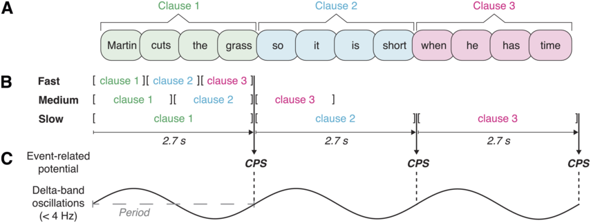
Implicit prosodic phrasing based on temporal processing windows of 2.7 seconds has also been found to influence syntactic parsing, in line with the behavioural evidence of working memory constraints on syntactic processing described above (e.g., Swets et al., Reference Swets, Desmet, Hambrick and Ferreira2007). When the time-induced prosodic phrasing pattern mismatches the expected syntactic parsing of a sentence, an ERP related to syntactic reanalysis (the so-called P600; Hagoort et al., Reference Hagoort, Brown and Groothusen1993) has been found, both in silent reading (Schremm et al., Reference Schremm, Horne and Roll2015) and speech processing (Henke and Meyer, Reference Henke and Meyer2021). Further evidence for a limited time window for the recoding of formal language features into semantics comes from an experiment on grammatical agreement (Roll et al., Reference Roll, Gosselke, Lindgren and Horne2013). Two (dis)agreeing words, such as We … run(s), were separated by four different time intervals based on increases in presentation rate. The temporal distances were below, at, or above 2.7 seconds. At the two faster rates, resulting in time intervals below 2.7 seconds, disagreeing elements produced the typical left anterior negativity (LAN) found for grammatical disagreement. This was interpreted as the processing of grammatical matching based on the form of the words. At a distance over 2.7 seconds, the negativity had a right-lateralized distribution, hinting at some other cognitive process being involved in matching the two elements, possibly semantically based. At 2.7 seconds, there was no effect of agreement, but participants’ working memory span correlated with the negativity in amplitude at the electrodes displaying the LAN. In favour of the idea that agreement processing at distances over 2.7 seconds rather involves semantic representations, a sharp divide in response times has been found for acceptability judgments of grammatical agreement with distances above or below 2.7 seconds. Yet, for semantic matching, response times instead slowly increased with presentation rate (Schremm et al., Reference Schremm, Horne and Roll2016).
Overall, time-driven processing constraints of approximately 2–3 seconds may shape the integration of words into larger multi-word groups. In particular, they may guide the insertion of implicit prosodic boundaries during reading, which allows the parsing of words into a syntactic structure before word traces fade from working memory. Semantic processing of language seems to be differently affected by this temporal constraint.
18.4 Neural Oscillations as Time Constraints?
Behavioural and ERP research both indicate a temporal constraint on the integration of words during language processing. Recently, it was hypothesized that this temporal limitation of processing windows discovered by the above behavioural and ERP work may stem from an underlying periodic electrophysiological substrate (Henke and Meyer, Reference Henke and Meyer2021; Meyer et al., Reference Meyer, Henry, Gaston, Schmuck and Friederici2016), so-called neural oscillations (cf. Chapter 3). Indeed, this work suggests that endogenous oscillatory activity may time-limit the duration of multi-word chunks, and it was also found to constrain acoustically driven chunking (Rimmele et al., Reference Rimmele, Poeppel and Ghitza2021). Cycles of low-frequency delta-band oscillations (<4 Hz) have a period of up to several seconds and are thus long enough to accommodate the integration of words into larger multi-word units. In that way, delta-band oscillations may function as an endogenous pacemaker for language processing (Meyer et al., Reference Meyer, Sun and Martin2020a, Reference Meyer, Sun and Martin2020b).
Delta-band oscillations have been associated with the tracking of prosody (Bourguignon et al., Reference Bourguignon, De Tiège and De Beeck2013; Gross et al., Reference Gross, Hoogenboom and Thut2013) but were also found to align with linguistic structure that is not apparent in the acoustic signal (Ding et al., Reference Ding, Melloni, Zhang, Tian and Poeppel2016; Meyer et al., Reference Meyer, Henry, Gaston, Schmuck and Friederici2016). Using isochronous stimuli, neural activity within the delta frequency band was found to track the rates of phrases and sentences, although those could not be inferred from the acoustic input (Ding et al., Reference Ding, Melloni, Zhang, Tian and Poeppel2016). Notably, tracking vanished when the phrasal rate fell out of the delta-band range (i.e., was faster; Lo, Reference Lo2021). Thus, delta-band oscillations may have an endogenous tempo playing an active role in language processing.
In natural language, it has proven difficult to investigate an endogenous function of delta-band oscillations because speech contains physical rhythms; even subtle acoustic cues may mask endogenous activity. Therefore, it is necessary to consider a different sensory domain that avoids this confound. In particular, text input does not provide any temporal structure on the chunk level; although punctuation may guide the structuring of the text input, punctuation marks occur in space and not at specific time intervals. Thus, rhythmic sampling during reading would be endogenously imposed. Accordingly, Henke et al. (Reference Henke, Lewis and Meyer2023) examined simultaneous recordings of eye movements and electroencephalography (EEG) during naturalistic reading and observed that fixation durations fluctuate rhythmically at ~1 Hz in coherence with delta-band activity over the occipital cortex.Footnote 4 This suggests that neural activity may impose its preferred processing pace onto reading, independent of physical rhythms in the stimulus. Complementary work on self-paced reading has shown that the behavioural periodicity of reading times (here, ~2 Hz) is temporally aligned to chunk boundaries – as defined by a computational formalization based on dependency annotations and part-of-speech tags – as well as sentence boundaries (Lo et al., Reference Lo, Anderson, Henke and Meyer2023). This alignment suggests that the observed periodicity is indeed related to the formation of multi-word chunks during language processing and may be behaviourally relevant to minimize memory demands. These findings on reading may also relate to psycholinguistic work on implicit prosodic phrasing (discussed in detail above). Implicit prosody as a chunking strategy may in fact be a reflection of underlying neural processing windows. Yet, as opposed to previously proposed integration windows of 2.7 seconds, the observed frequencies of 1–2 Hz in reading suggest rather short time windows of 0.5–1 second. These shorter and longer time windows could relate to the multi-scale nature of prosody that comprises both intermediate as well as full prosodic phrases (Stehwien and Meyer, Reference Stehwien and Meyer2022). In particular, multiple short intermediate phrases may be integrated into longer prosodic phrases. Alternatively, the size of the integration windows may differ across modalities; for instance, the here reported results suggest shorter windows for visual as compared to auditory language processing. More work is needed to unravel the different time windows and their underlying neural implementation.
Returning to the longer integration windows and supporting the idea of an endogenous constraint of electrophysiological processing, the phase of delta-band oscillations was found to predict the termination of multi-word chunks (Meyer et al., Reference Meyer, Henry, Gaston, Schmuck and Friederici2016) and, more specifically, to enforce chunking after 2.7 seconds (Henke and Meyer, Reference Henke and Meyer2021). These studies employed ambiguous sentences similar to those used in the behavioural psycholinguistic studies described above. The results suggest that chunking, and as a consequence attachment, is affected by the phase of delta-band oscillations. Reconsidering the behavioural results from this perspective, it may be that the period of these oscillations subserves (implicit) prosodic phrasing (Glushko et al., Reference Glushko, Poeppel and Steinhauer2022) and underlies the different chunking strategies of the high and low working memory span groups described above (i.e., the high-span group integrates more information together, while the low-span group terminates a chunk earlier; Swets et al., Reference Swets, Desmet, Hambrick and Ferreira2007). Note here that the duration of the chunking window for delta-band oscillations also aligns with findings on the CPS (e.g., Roll et al., Reference Roll, Lindgren, Alter and Horne2012) described above. Based on this, it was suggested that the CPS may consist of underlying neural oscillations within the delta band (Meyer et al., Reference Meyer, Henry, Gaston, Schmuck and Friederici2016); the increased amplitude that is observed as ERP may arise from phase-locking of oscillatory activity across trials (Sauseng et al., Reference Sauseng, Klimesch and Gruber2007). Yet, to date, this remains to be shown (see Inbar et al., Reference Inbar, Genzer, Perry, Grossman and Landau2023, for the first evidence consistent with a relationship between the CPS, prosodic boundaries, and delta-band tracking during naturalistic speech listening).
As mentioned previously, delta-band oscillations may also be exogenously guided by prosody (see Chapter 15 for further discussion on exogenous versus endogenous influences within the delta band), aligning their phase to slow modulations in the acoustic speech signal (e.g., Bourguignon et al., Reference Bourguignon, De Tiège and De Beeck2013; Ding and Simon, Reference Ding and Simon2014; Gross et al., Reference Gross, Hoogenboom and Thut2013). Strikingly, oscillations were also found to inherit the exogenous stimulus frequency, so that the aligned oscillatory rhythm persists even after stimulus offset – a phenomenon called entrainment (Kösem et al., Reference Kösem, Bosker and Takashima2018; Luo and Poeppel, Reference Luo and Poeppel2007; Obleser and Kayser, Reference Obleser and Kayser2019). Entrainment thus results from an exogenous (acoustic) cue, which then affects subsequent processing from the inside out. For instance, presenting participants acoustically with repetitive prosodic contours – whose duration fell within the delta-band range – influenced the perception of subsequently presented sentences that either matched or did not match the duration of the prosodic contours (Lamekina and Meyer, Reference Lamekina and Meyer2023). When their duration matched, processing of the visually presented sentences was facilitated as indicated by decreased response times in behaviour. This indicates that the prosodic contours lead to a temporal prediction of the upcoming sentence duration, possibly driven by entrained delta-band oscillations. Notably, the facilitatory effect was numerically strongest for prosodic contours of 2.5 seconds as compared to shorter (1.5 seconds) or longer contours (3.5 seconds). Supporting the role of the delta band as a pacemaker for processing, entrainment may be strongest when the exogenous stimulus matches the preferred endogenous pace.
While we propose that the period of oscillatory cycles at delta-band frequency imposes a temporal constraint on chunk-level integration, the course of each individual cycle may yet pose another constraint on processing: Excitability of the underlying cells changes along the course of the cycle and hence processing abilities are not uniform. On the neuronal level, there are excitable phases, where processing is facilitated, and unexcitable phases that hinder processing (Lakatos et al., Reference Lakatos, Shah and Knuth2005). A promising avenue for future research is to assess whether these cycles of excitability are aligned to the expected informativeness of the incoming language input, following the sentence’s information structure. For example, prosodic and syntactic cues to upcoming information structure may phase-reset ongoing delta-band oscillations so that the more excitable phase of the oscillations will coincide with the expected timing of more important, new information, while the less excitable phase will occur during less important, given information. Further research is needed to address this and similar questions regarding the relationship between oscillatory cycles of excitability and higher-order language processing.
In conclusion, delta-band oscillations may underlie the previously proposed time constraint and serve as an endogenous pacemaker for language processing. In particular, their preferred wavelength may constrain the formation of multi-word chunks, and even alignment to an external stimulus may be best when the stimulation duration matches their preferred endogenous pace. Additionally, excitability gradients along the cycle may yet pose another timing constraint on the processing of the information structure of the input.
18.5 Discussion
Converging findings from behaviour, ERPs, and oscillatory research point towards temporal constraints on linguistic processing. These constraints can either be context-dependent, resulting from the available linguistic and acoustic information, or context-invariant, representing endogenous processing limitations.
The psycholinguistic literature indicates that (implicit) prosody, syntax, and information structure interact in guiding the formation of multi-word chunks. During speech comprehension, acoustic cues of the prosodic structure guide syntactic parsing through the alignment of prosodic and syntactic boundaries. Even in silent reading, comprehenders use implicit prosodic structure as a chunking strategy to support syntax; this is in line with ERP evidence on the CPS during silent reading. Prosody and syntax further constrain linguistic processing by acting as cues to the information structure of a sentence, guiding attention and processing resources towards the timing of important information.
Additionally, studies on (implicit) prosodic phrasing provide evidence for a specific temporal limit on language production and comprehension. In particular, a context-independent temporal constraint of approximately 2–3 seconds shapes the integration of words into larger multi-word chunks. These temporal integration windows may reflect cognitive and neural processing limitations. At this point, there is no evidence that can disentangle the nature of these limitations; that is, whether they may result from the decay function of working memory or low-frequency delta-band oscillations. However, these accounts may not be mutually exclusive: Oscillatory cycles could potentially be the electrophysiological unit that corresponds to the working memory buffer that binds multiple to-be-integrated words during language comprehension. Indeed, temporal processing constraints have also been related to inter-individual differences in working memory capacity (Roll et al., Reference Roll, Lindgren, Alter and Horne2012, Reference Roll, Gosselke, Lindgren and Horne2013). Likewise, from an oscillatory perspective, a static cycle duration will find little support in terms of ecological validity for language processing. Hence, oscillatory cycles will likely be flexible within a certain frequency range and may vary across individuals. Furthermore, it remains open if this temporal constraint applies in the same way to different levels of processing. While temporal constraints directly seem to affect prosodic and syntactic processing, effects at higher levels of processing such as semantics or information structure may only be indirectly induced by lower-level constraints on chunking.
Contrary to the idea of a temporal constraint discussed here, it may also reflect an information constraint. Cross-linguistic research has found similar information rates for syllables across languages (Coupé et al., Reference Coupé, Oh, Dediu and Pellegrino2019; Pellegrino et al., Reference Pellegrino, Coupé and Marsico2011), suggesting a close relationship between the speech production rate and the informativeness. This information rate may be optimally tuned to our processing capacity. In this way, there may be a limit to the amount of information that can be processed within an integration window, which in turn may determine chunking behaviour. Limitations on information processing would also be consistent with the idea that speakers prefer utterances that convey information uniformly across speech signals (Entropy Rate Constancy/Uniform Information Density Hypothesis; Genzel and Charniak, Reference Genzel and Charniak2002; Jaeger, Reference Jaeger2010; Xu and Reitter, Reference Xu and Reitter2018).
Future studies may address these questions by combining measures from cognitive neuroscience with psycholinguistic paradigms to tease apart the specific neural processes underlying language comprehension (Beier et al., Reference Beier, Chantavarin, Rehrig, Ferreira and Miller2021; Meyer et al., Reference Meyer, Sun and Martin2020b).
Summary
We present evidence for temporal constraints on (implicit) prosody, syntax, and information structure. These constraints may link to cognitive and neural (e.g., oscillatory) processing limitations and interact with the buildup of structure during comprehension. We suggest that these constraints shape linguistic structure at an optimal pace for brain processing.
Implications
Cognitive, neural, and linguistic timing constraints influence language processing, either contextually or context-invariantly. These constraints appear to interact with the physical timing of the speech signal in shaping the timing of processing. We thus recommend to take them into account when designing experiments and interpreting findings on speech/language processing.
Gains
We review evidence for context-dependent and context-invariant timing influences on language processing. This may help to acknowledge that behavioural and neural rhythms during language processing – and possible speech and language as such – are shaped both exogenously by speech timing and endogenously by cognitive, neural, and linguistic constraints.
19.1 Introduction
One fundamental constraint on natural language is that, while linguistic representations are hierarchical, words have to be produced (and heard) one after the other. Many cognitive scientists argue this requires that speakers and hearers map the hierarchical information associated with sentences and their meanings into (and from) linearized strings of linguistic material while minimizing ambiguity and information loss. This mapping is made possible by the complex interaction of word order, morphology, and prosody. At the prosodic level, duration (the focus of this chapter), together with pitch and intensity, contributes both to speech segmentation (e.g., to identify word boundaries) and to grouping words into hierarchically organized prosodic representations (partially) mapping into underlying syntactic structures and their semantic interpretation.
Our ability to use durational information for speech disambiguation depends in turn on the ability to track the rhythmic properties of speech, as defined in this volume. For example, while speech rate itself does not carry grammatical information, it largely shapes our perception of both segmental and suprasegmental features, leading us to perceive the same speech sounds as being longer in the context of faster speech rate and shorter in the context of slower speech rate.Footnote 1 In other words, speech rate provides a baseline against which we can evaluate the durational properties of segmental and suprasegmental information against our predictions of their expected duration at that specific rate. At segmental level, effects of rate normalization have been reported for, as examples, voice onset time (Miller and Grosjean, Reference Miller and Grosjean1981; and others), vowel length (Reinisch and Sjerps, Reference Reinisch and Sjerps2013; and others), and word segmentation (Salverda et al., Reference Salverda, Dahan and McQueen2003; Reinisch et al., Reference Reinisch, Jesse and McQueen2011). Similarly, in the domain of phrasal prosody, the realization and interpretation of prosodic boundaries have also been shown to be contextually dependent in production and their interpretation in parsing (on the importance of relative versus absolute values in the perception of boundaries, see, for example, Schafer, Reference Schafer1997; Carlson et al., Reference Carlson and Frazier2001; Clifton Jr et al., Reference Carlson and Frazier2002; Frazier et al., Reference Frazier and Carlson2006; and others).
The durational properties of speech, however, are not only determined by structural factors but can also be modeled as a function of predictability: Less predictable words and segments are typically produced more slowly, and more predictable material is produced more quickly. Considerations of predictability and structure often make aligned predictions in relation to duration (e.g., in the domain of focus or in the case of early closure discussed below). To distinguish the relative contribution of these two factors, we identified a case in which the two factors make opposite predictions: the contrast between structural sisterhood (e.g., The horse raced past the barn and fell) and nesting (e.g., The horse raced past the barn fell). It is well established that nested structures are harder to process and understand (at least out of the blue) than sisterhood structures. While the source of the so-called garden path effects triggered by nesting is still a contentious matter, predictability-based accounts have become increasingly more prominent in psycholinguistics (Hale, Reference Hale2001; Levy, Reference Levy2008).
The main aim of this chapter is to argue that there are well-defined sets of environments for which lower predictability is in fact associated with shorter duration due to prosodic principles taking precedence over predictability in shaping the durational properties of speech. After briefly summarizing the role of prosodic structure and predictability in duration, we report on four recent studies showing that an inverse relation between duration and complexity is observed in the prosodic disambiguation of nested garden path sentences in production and comprehension. Specifically, the results of these studies show that, across different syntactic categories, nested garden path sentences are exceptional in displaying a relatively faster tempo when disambiguated towards less predictable structures. The important conclusion here is that, while predictability plays an important role in modulating duration, when in conflict with prosody, prosodic structure takes precedence.
We see the acceleration of a speech rhythm baseline as a hallmark of structural nesting in garden path sentences, and we suggest an account in which this change of tempo stems from an interaction between two types of principles: principles governing the syntax–prosody mapping, and principles balancing the size of prosodic phrases.Footnote 2 Nesting naturally generates a conflict between these two types of principles: Syntactically and semantically, it creates complex objects that should ideally be prosodified as a single constituent. This, however, would result in longer phrases, which can be difficult to manage for balancing principles. One solution is to break these long syntactic objects into separate prosodic phrases (as in extraposition; Wagner, Reference Wagner2005, Reference Wagner2010). We argue that nested garden path sentences, however, are unique in preventing nested elements from being prosodically separated from their hosts. In these structures the need for balance is satisfied by an increasing tempo of the long phrase. This solution increases parsability of nested garden paths while satisfying both types of principles. In essence, the prosodic pattern of nested garden path sentences exemplifies how different levels of representation interact and impact the rhythmic properties of speech. In simpler terms, disrupting the rhythm of speech at a lower level (tempo acceleration) helps create a smoother rhythm at a higher level (balanced prosodic phrases).
19.1.1 Duration and Prosodic Structure
We will follow the common assumption that prosodic structures constitute an independent level of representation. In this perspective, prosody can be understood as the structure that determines and organizes the acoustic realization of an utterance in relation to its phrasing (the chunking of speech) and (lexical and post-lexical) prominence configuration, among other aspects of speech (i.e., voice quality, rate; Selkirk, Reference Selkirk1980; Beckman and Pierrehumbert, Reference Beckman and Pierrehumbert1986; Nespor and Vogel, Reference Nespor and Vogel2007). Prosodic structure is conceived as a grammatical system, made of hierarchically ordered constituents, that is distinct from syntactic structure (but see other approaches to the prosody–syntax interface; Cooper and Paccia-Cooper, Reference Cooper and Paccia-Cooper1980; Gee and Grosjean, Reference Gee and Grosjean1983) and is universal (with the implementation of language-specific adjustments). Figure 19.1 schematizes prominence and phrasing-related constituents of the prosodic structure as posited by well-known phonological accounts of prosody (i.e., the autosegmental-metrical [AM] framework; Pierrehumbert, Reference Pierrehumbert1980; Beckman and Pierrehumbert, Reference Beckman and Pierrehumbert1986; Ladd, Reference Ladd1986) and described using notational conventions such as the ToBI (Tones and Break Indices) transcription system (Silverman et al., Reference Silverman, Beckman and Pitrelli1992; Beckman and Ayers, Reference Beckman and Ayers1997).
Prosodic hierarchy.
Schematic representation of the prosodic hierarchy. “IP” stands for intonational phrase (demarcated by boundary tones “T %”) and “ip” for intermediate phrase (demarcated by phrase accents “T-”) grouping words (“ω”) and syllables (“σ”). T* stand for pitch accents realized on lexically stressed syllables.
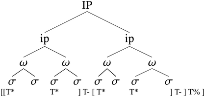
While syntax and prosodic structure are not isomorphic, the relative degree of structural and interpretive integration of linguistic elements is one strong determinant of an utterance’s prosodic structure. Principles governing the interface of prosody and syntax, such as edge alignment (Selkirk, Reference Selkirk and Horne2000) and wrap (Truckenbrodt, Reference Truckenbrodt1995), push for prosodic phrasing to align with syntactic phrases as much as possible.
Edge alignment:
“The right edge of any syntactic phrase (XP) in syntactic structure must be aligned with the right edge of a Major Prosodic Phrase in prosodic structure.” (Selkirk, Reference Selkirk and Horne2000, p. 232)
Wrap:
“Each syntactic XP must be contained in a phonological phrase.” (Truckenbrodt, Reference Truckenbrodt1995, p. 10)
Within the realm of duration, pre-boundary lengthening (for English; Klatt, Reference Klatt1976; Wightman et al., Reference Wightman, Shattuck-Hufnagel, Ostendorf and Price1992), pauses (Watson and Gibson, Reference Watson and Gibson2005; Breen et al., Reference Breen, Watson and Gibson2011), and domain-initial strengthening (Cho and Keating, Reference Cho and Keating2009) are the main phenomena in which duration determines whether a boundary is perceived and what strength is associated with it (see the discussion in Wagner and Watson, Reference Wagner and Watson2010; Turk and Shattuck-Hufnagel, Reference Turk and Shattuck-Hufnagel2014; Dahan, Reference Dahan2015, and references cited therein).
For our purposes, a good illustration of how duration guides prosodic grouping at the phrasal level across both production and comprehension comes from Kjelgaard and Speer’s (Reference Kjelgaard and Speer1999) work on the disambiguation of garden path sentences such as (1). In (1a) (i.e., the most accessible interpretation in the absence of prosodic disambiguation), the verb leaves is interpreted transitively and forms a single phrase with the following determiner phrase (DP) the house, which is followed by a prosodic break (indicated with “||” here). In (1b) the same verb is interpreted intransitively, and it constitutes the final region of the temporal modifier when John leaves. This region is immediately followed by a prosodic boundary that signals that the following DP the house should not be integrated in the same phrase but should be interpreted as the subject of the following predicate is dark. This parse is strongly dispreferred in the absence of prosodic information or punctuation. The preference for interpreting the verb transitively (as in 1a) can alternatively be interpreted as part of a generalized parsing preference to incorporate incoming words into the phrase being processed whenever grammatically possible (late closure strategy; Frazier, Reference Frazier1979) or as generated by the relative higher frequency of transitive versus intransitive readings of verbs such as leaves (Tanenhaus et al., Reference Tanenhaus, Carlson and Trueswell1989; MacDonald et al., Reference MacDonald, Pearlmutter and Seidenberg1994).
(1)
a. When John leaves the house || it’s dark. Late closure b. When John leaves || the house is dark. Early closure
Kjelgaard and Speer show that lengthening of the pre-boundary word leaves in (1b), compared to when the same word occurs in phrase-medial position in the late closure example in (1a), helps listeners avoid a garden path effect, even in the absence of an actual pause between the verb and the following DP. It is important to stress that what is critical for disambiguation is information about relative duration: The presence of a boundary in a given region will be a matter of relative duration of a given segment, not of the absolute durational properties of that segment. For a detailed discussion of how the importance of relative duration and global, rather than local, measures support a role for prosodic representations, see, for example, Schafer (Reference Schafer1997); Carlson et al. (Reference Carlson and Frazier2001); Clifton Jr et al. (Reference Carlson and Frazier2002); Frazier et al. (Reference Frazier and Carlson2006); Shatzman and McQueen (Reference Shatzman and McQueen2006); Speer and Blodgett (Reference Speer, Blodgett, Traxler and Gernsbacher2006).
Constraints favoring the alignment of syntactic and prosodic phrasing, however, operate in tandem with other eurythmicFootnote 3 or balance constraints, which ensure, for example, that prosodic phrases do not exceed a certain size in production, and are preferably parsed into units of similar length in comprehension (Frazier and Fodor, Reference Frazier and Fodor1978; Gee and Grosjean, Reference Gee and Grosjean1983; Ghini, Reference Ghini1993; Fodor, Reference Fodor2002).
Binary minimum:
“A major phrase must consist of at least two minor/accentual phrases.” (Selkirk, Reference Selkirk and Horne2000)
Binary maximum:
“A major phrase may consist of at most two minor/accentual phrases.” (Selkirk, Reference Selkirk and Horne2000)
Uniformity:
“A string is ideally parsed into same length units.” (Ghini, Reference Ghini1993)
Conflicts can arise between these different constraints and generate mismatches between syntactic and prosodic phrasing such as the one in (2) and (3) (adapted from Turk and Shattuck-Hufnagel, Reference Turk and Shattuck-Hufnagel2014, p. 2):
(2) Syntactic structure:
[This is [the cat [that ate [the rat [that ate the cheese]]]]]
(3) Prosodic structure:
[This is the cat] [that ate the rat] [that ate the cheese].
The extent of syntax–prosody mismatch is rather controversial (for a recent summary, see Bennett and Elfner, Reference Bennett and Elfner2019) and outside the immediate scope of this chapter, so we will not devote a long discussion to it. But to appreciate the debate, note that some researchers (e.g., Wagner, Reference Wagner2005, Reference Wagner2010) suggest that true instances of a mismatch might be more limited than standardly assumed, and that cases such as (2) and (3) can be accounted for by extraposition of the relative clauses (RCs), such that they attach to a higher position in the syntactic structure and provide a much tighter alignment between prosodic and syntactic structures. Whatever the correct account for these and other similar contrasts, they serve well to illustrate the tension between syntax–prosody mapping and eurhythmic principles, an issue we’ll return to below when discussing the prosodic properties of nested garden path sentences.
19.1.2 Duration and Predictability
Durational properties of speech have also been shown to be largely dependent on predictability. More predictable words/segments are reliably associated with a shorter production duration. Less predictable elements of utterances, on the other hand, are more carefully articulated, and thus produced more slowly (Lieberman, Reference Lieberman1963; Aylett, Reference Aylett2000; Jurafsky et al., Reference Jurafsky, Bell, Gregory and Raymond2001; Aylett and Turk, Reference Aylett and Turk2004; Turk and Shattuck-Hufnagel, Reference Turk and Shattuck-Hufnagel2014; Levy and Jaeger, Reference Levy and Jaeger2007; and others).
For example, syllables in words that carry new or contrasting information, and are thus less predictable, are typically associated with prosodic prominence, making them louder, longer, and articulated more carefully (Aylett, Reference Aylett2000; Aylett and Turk, Reference Aylett and Turk2004; Watson et al., Reference Watson, Arnold and Tanenhaus2008; Turk and Shattuck-Hufnagel, Reference Turk and Shattuck-Hufnagel2014).Footnote 4 Aylett (Reference Aylett2000) and Aylett and Turk (Reference Aylett and Turk2004) suggest an information theoretic account of these observations, the smooth signal redundancy hypothesis, according to which the inverse relation between duration and predictability “provides an efficient way of ensuring that elements with low levels of language redundancy are produced for a longer period of time and perhaps with more salient acoustic characteristics, and will thus be likely to be recognized” Aylett and Turk (Reference Aylett and Turk2004, p. 33). This is illustrated in (4), where the words pizza and John are associated with longer duration when in focus. It is also well known that elements in prosodically prominent positions receive more attention, are remembered better, and are processed faster than non-prominent elements (Cutler, Reference Cutler1976, Reference Cutler2012).Footnote 5
a. What does John like? John likes PIZZA.
b. Who likes pizza? JOHN likes pizza.
Similar considerations apply to the domain of syntactic phrasing, where more predictable parses are expected to be produced faster than less predictable ones. The early closure garden path sentence discussed above (and repeated in 5) provides a good illustration of this. As mentioned, according to one analysis of early closure, the intransitive reading in (5b) is harder to parse because it is less predictable, for example, because it is encountered less frequently, than the transitive reading in (5a) (Tanenhaus et al., Reference Tanenhaus, Carlson and Trueswell1989; MacDonald et al., Reference MacDonald, Pearlmutter and Seidenberg1994). A predictability account would assume that a longer duration of the ambiguous region (leaves the house) would help listeners to resolve the ambiguity towards the less predictable parse (presumably by positing a boundary between leaves and the house).
a. When John leaves the house || it’s dark.
b. When John leaves || the house is dark.
As this example illustrates, the same durational difference could in principle be correctly predicted on the basis of both prosodic structure and predictability (i.e., longer duration at leaves for early closure than late closure). In many instances of ambiguity, it would indeed seem that the effects on production of both prosodic structure and predictability are essentially aligned: “when predictability is low, syllables are more likely to be prosodically prominent, and words are more likely to be demarcated using prosodic boundary correlates such as initial- and final-lengthening and pause” (Turk and Shattuck-Hufnagel, Reference Turk and Shattuck-Hufnagel2014, p. 4). However, as Turk and Shattuck-Hufnagel (Reference Turk and Shattuck-Hufnagel2014, p. 4) also point out, “the problem with predictability as a factor affecting duration is that it is unclear whether prosodic structure and predictability are both motivated as separate and independent factors affecting duration. This is because prosodic structure and predictability are not independent.”
To dissociate the relative contribution of predictability and prosodic structure, it is important, therefore, to focus on cases in which these two factors make opposite predictions. In recent work (Grillo and Turco, Reference Grillo and Turco2016; Grillo et al., Reference Grillo, Aguilar, Roberts, Santi and Turco2018, Reference Grillo, Aguilar, Roberts, Santi and Turco2019), we have suggested that the contrast between sisterhood and nesting is one such case.
19.2 Prosody and Predictability Make Opposite Predictions for Nested Garden Paths
The structural ambiguity of nesting versus sisterhood is extremely common and has been one of the main testing grounds for different theories of sentence processing. The sentences in (6) are a few examples of well-described cases of locally ambiguous sentences involving this structural ambiguity. As shown by the bracketing, the first example of each pair of sentences illustrates nesting: The ambiguous phrase is embedded within the constituent it modifies and forms a single syntactic phrase with it. The second example of each sentence pair illustrates sisterhood: In these examples the ambiguous phrase is a sister constituent to the preceding constituent. For each set of examples, the nested reading has been shown to generate longer reading times at the disambiguation region and poorer comprehension (at least out of the blue) than the sisterhood reading (see, for example, Pickering and Van Gompel, Reference Pickering, Van Gompel, Traxler and Gernsbacher2006, for a review).Footnote 6
(6)
a. [[The horse [raced past the barn]] fell] Reduced relative b. [[The horse] [raced past the barn] and [fell]] Main verb c. John [told [the man [that he was running with]] [to wait]] RC d. John [told [the man] [that he was running with Max]] CC e. [Put [the horse in the barn] [on the truck]] Restrictive PP f. [Put [the horse] [in the barn]] Goal PP g. John [saw [the man [with the binoculars]]] Restrictive PP h. John [saw [the man] [with the binoculars]] Instrumental PP
While the source of this contrast in processing difficulty is still a contentious matter, an increasingly prominent perspective in psycholinguistics is that nested structures are harder to parse because they are less predictable. This approach is supported by corpus studies and computational modeling. Hale (Reference Hale2001), for example, shows that the reduced relative parse in (6a) is seven times less likely to occur in a corpus than the simpler analysis involving the unmodified noun phrase. Similarly, Jurafsky (Reference Jurafsky1996), based on data from Connine et al. (Reference Connine, Ferreira, Jones and Frazier1984), combined syntactic probability of the main verb and reduced-RC parse (and the related lexical probability of the intransitive versus transitive reading of the verb raced in the horse raced past the barn (and) fell) to estimate “the probability ratio of the two analyses of pre-disambiguation context … as roughly 82:1” (Levy, Reference Levy, Lin, Matsumoto and Mihalcea2011).
From an information theoretic perspective, therefore, longer reading times observed in processing studies for nested structures are seen as a function of lower predictability. As with production, studies on sentence processing show an inverse relationship between redundancy and duration. Structural analyses entertained at earlier regions of a sentence generate structural expectations about parts of the sentence that are yet to come (Konieczny, Reference Konieczny2000; Hale, Reference Hale2001; Lau et al., Reference Lau, Stroud, Plesch and Phillips2006; Staub and Clifton, Reference Staub and Clifton2006; Levy, Reference Levy2008; Levy et al., Reference Levy, Fedorenko, Breen and Gibson2012; Traxler, Reference Traxler2014; Kuperberg and Jaeger, Reference Kuperberg and Jaeger2015). The amount of time spent reading a particular region is a function of the strength of prior expectations.
If the durational properties of speech are primarily determined by predictability, we should expect the lower predictability of nested garden paths to lead to longer durations in production than string-identical sentences involving more predictable sisterhood structures. This perspective should generate similar predictions for comprehension as well: A longer produced duration of the ambiguous region should make it easier for listeners to parse structural nesting; a shorter produced duration, on the other hand, should aggravate the garden path effect as it would be taken to map onto the more predictable sisterhood structure.
Importantly, considerations of prosodic structure generate the opposite predictions in relation to both production and comprehension of nested garden paths, leading us to expect a shorter duration for nesting than sisterhood in production, which translate into facilitated processing, that is, a reduction in the garden path effect for nesting when comprehending an ambiguous phrase produced with a relatively shorter duration. These predictions are based on the relative degree of structural (and interpretive) integration of nesting and sisterhood and the constraints on prosodic structure introduced above.
Sister constituents are independent phrases and attach higher in the syntactic structure than nested constituents. This syntactic difference makes sister constituents more likely to be produced as separate prosodic phrases than nested constituents, which are contained within the XP they modify, and are thus more likely to be mapped onto a single prosodic phrase (following the principles of edge alignment and wrap). Indeed, it is well established that a higher attachment site correlates with separate phrasing, and given that prosodic phrasing modulates the durational properties of utterances in predictable ways (e.g., pre- and post-boundary lengthening), separate phrasing typically leads to longer durations for attachment to higher positions and shorter durations for more deeply embedded strings (Hirschberg and Avesani, Reference Hirschberg and Avesani1997; Clifton Jr et al., Reference Carlson and Frazier2002; Wagner and Watson, Reference Wagner and Watson2010; Poschmann and Wagner, Reference Poschmann and Wagner2015; Grillo and Turco, Reference Grillo and Turco2016; among many others).
Given the differences in attachment site of sister and nested constituents, we can predict that sister constituents are more likely to be produced as separate phrases than nested constituents. In turn, this leads us to predict a longer duration for sisterhood structures at the regions preceding and following the phrase boundary, despite their higher predictability.Footnote 7
The example from nested garden paths involving prepositional phrases (PPs) in (6e) versus (6f), repeated below, illustrates these effects very appropriately. These sentences have been consistently shown to be prosodically disambiguated (Snedeker and Trueswell, Reference Snedeker and Trueswell2003; Kraljic and Brennan, Reference Kraljic and Brennan2005; Schafer et al., Reference Schafer, Speer, Warren, White, Trueswell and Tanenhaus2005; Speer et al., Reference Speer, Warren and Schafer2011). Importantly, a stronger prosodic boundary between the DP (the horse) and the PP (in the barn) leads to a longer duration of both regions in the more predictable and easier to parse sisterhood condition (7a) than in the less predictable nested structure in (7b).
a. [Put [the horse] [in the barn]].
b. [Put [the horse [in the barn]] [on the truck]].
While this prosodic pattern is well attested, no work to date to our knowledge has attempted to integrate these results within a predictability account of duration. More generally, despite the central role played by nested garden paths in guiding psycholinguistic theories, until recently there has been surprisingly little experimental evidence on how the contrasts in (6) are prosodically disambiguated in production and comprehension.Footnote 8 A comprehensive study of the prosody of sisterhood versus nesting garden path sentences is still lacking. This is probably also due to the widespread assumption that some of these ambiguities (e.g., main verb versus reduced relatives) are not prosodically disambiguated (see, for example, Fodor, Reference Fodor2002; Wagner and Watson, Reference Wagner and Watson2010).
19.2.1 Reduced-RC Garden Paths
Recent results from our research group support the prediction that nested garden path sentences are associated with a shorter duration than the sisterhood structure, despite nesting being more difficult to parse out of the blue (and, at least in some cases, less predictable because of their lower frequency). In this section we review these results, and in the following section we will review our theoretical interpretation of these durational effects. In Grillo et al. (Reference Grillo, Aguilar, Roberts, Santi and Turco2018) we investigated the prosodic disambiguation of classic garden path sentences that are temporarily ambiguous between a main verb and a reduced-RC verb (6a, b)]. This type of garden path is generated by the ambiguity between a past tense and a passive past participle reading of the verb raced. As mentioned, we predicted that a difference in attachment height of the verb phrase (VP) (raced past the barn) with respect to the subject DP (the horse) should lead to shorter duration for the less predictable reduced-RCs. As explained above, the rationale for these predictions comes from the simple observation that the ambiguous string forms a single constituent in the reduced-RC analysis, but two separate syntactic phrases in the main verb analysis.
We also suggested that prosodic disambiguation of this type of contrast might have previously gone unnoticed because these sentences were typically presented in isolation and started with the critical pre-boundary ambiguous region. This is a problem because, as mentioned above, the absolute durational properties of the ambiguous region are not informative in isolation, but only when evaluated in relation to a baseline tempo provided by linguistic material preceding the ambiguous region itself (Schafer, Reference Schafer1997; Carlson et al., Reference Carlson and Frazier2001; Clifton Jr et al., Reference Carlson and Frazier2002; Frazier et al., Reference Frazier and Carlson2006).
In Grillo et al. (Reference Grillo, Aguilar, Roberts, Santi and Turco2018) we used the Planned Production paradigm to test these hypotheses. In Planned Production, participants are instructed to silently scan the entire sentence before producing them naturally and fluently at normal speed. All stimulus sentences were preceded by a short introductory main clause (Greg said that in (8)) that was neutral with respect to the relevant disambiguation, but provided a baseline tempo against which the durational properties of the ambiguous region could be evaluated:Footnote 9
a. Main verb condition:
Greg said that [TP [DP the businessmen] [VP loaned money at low interest] and [VP were told to record their expenses]].
b. Reduced-RC condition:
Greg said that [TP [DP the [NP businessmen [CP loaned money at low interest] [VP were told to record their expenses]]].
The results showed that the contrast in (8) is prosodically disambiguated, and that this disambiguation can be detected as early as the subject DP (the businessmen). We found the ambiguous region (the businessmen loaned money at low interest) to be shorter in the less predictable RC condition (8a) than the more predictable main clause condition (8b). This difference was visible both in terms of absolute and relative duration, calculated as the ratio of the ambiguous region duration to that of the intro clause (Greg said that). Speech rate increased significantly more for the less predictable nested condition than for the sisterhood condition. These durational differences cannot be accounted for from a predictability perspective, as they contradict the predictions it would make. Instead, they reflect the distinct structural relation between the DP and the VP in these sentences.
In a follow-up forced-choice comprehension study (Grillo et al., Reference Grillo, Santi, Aguilar, Roberts and Turco2022), one of the participants’ recordings from the Planned Production study of Grillo et al. (Reference Grillo, Aguilar, Roberts, Santi and Turco2018) were used to test the extent to which listeners use these prosodic cues to overcome the garden path effect. The disambiguating region was removed from the recordings of both the main verb and the reduced relative conditions. To test the hypothesis that the presence of a baseline tempo is essential to the interpretation of the temporal properties of the ambiguous region (i.e., to the interpretation and disambiguation of the boundary between the businessmen and loaned money at low interest in (8)), we also manipulated whether an introductory clause was present (9a–b) or not (9c–d):
a. Reduced-RC prosody – baseline:
Greg said that the businessmen loaned money at low interest …
b. Main verb prosody – baseline:
Greg said that the businessmen loaned money at low interest …
c. Reduced-RC prosody – no baseline:
The businessmen loaned money at low interest …
d. Main verb prosody – no baseline:
The businessmen loaned money at low interest …
The same durational (and more generally prosodic) differences (in absolute terms) are present in both pairs of sentences; that is, identical recordings are used for condition A and C, on the one side, and for conditions B and D, on the other. The only difference between the two is the presence of an introductory sentence, providing a slower baseline tempo, which was removed from the recording in conditions C and D.
Participants listened to the cropped recording and then selected between two alternative continuations (main verb versus reduced-RC) that were written on the screen. In line with previous results from the garden path literature, a strong preference for the main verb continuation was found across all conditions. Main verb-compatible continuations constituted approximately 80% of choices in both full (baseline present) and cut (baseline absent) main verb conditions. The reduced relative continuation, nevertheless, was chosen twice as often when the RC prosody was preceded by an introductory clause to provide a baseline tempo. This is predicted by our approach since without a baseline tempo it should be impossible to decide whether the durational properties of the ambiguous region should be taken to indicate lengthening/lack of lengthening. A much more likely outcome is that they will be taken to reflect grammatically uninformative absolute speech rate. We thus correctly predict a smaller garden path effect when reduced-RCs are embedded within a main clause providing a baseline rate.Footnote 10
19.2.2 CC/RC Ambiguity
More recently, Grillo et al. (Reference Grillo, Aguilar, Roberts, Santi and Turco2023) showed that speakers similarly use temporal cues to prosodically disambiguate the complement clause (CC) versus RC garden path (10). The complementizer phrase (CP) that he was singing with is initially temporarily ambiguous between being a modifier (i.e., an RC) (10a) or a co-argument (i.e., a CC) of the DP, the editor (10a).
a. RC
The kind lyricist [V′ told [DP the [CP [NP editor [C′ that he was singing with]]]] [CP to listen]].
paraphrasable as: what the kind lyricist told the editor that he was singing with was to listen
b. CC
The kind lyricist [VP [V′ told [DP the [NP editor]] [CP that he was singing with Lola]]].
paraphrasable as: what the kind lyricist told the editor was that he was singing with Lola
The results of the Planned Production study showed that the ambiguous region (the editor that he was singing (with)) is associated with faster tempo when nested (the RC in (10a)) than when in a sisterhood relation (the CC in (10b)). In line with what we observed with reduced-RCs, this pattern was not only visible in raw durations (in ms) but also, and more importantly, in the change in speech rate between the intro phrase (the kind lyricist told) and the ambiguous region (the editor that he was singing with). Predictably, this pattern reversed at the final word of the ambiguous region (the preposition with), which precedes a major prosodic boundary in the RC condition.
Notice that we do not mean to suggest that tempo modulation is solely responsible for disambiguation of these structures. As can be clearly seen in Figure 19.2 (C, D), clear differences in pitch and intensity also differentiate the two readings (which is also supported by a ToBI analysis presented in Grillo et al., Reference Grillo, Aguilar, Roberts, Santi and Turco2023). What is important for the present discussion is that the prosodic structure of RCs leads to (among other things) shorter duration, despite their lower predictability.
Spectrograms of nested garden path sentences.
Example of waveform, spectrogram, and fundamental frequency (F0) track of main verb (A), reduced-RC (B), CC (C), and RC (D) structures; recorded by British English native informants in Grillo et al. (Reference Grillo, Aguilar, Roberts, Santi and Turco2018, Reference Grillo, Aguilar, Roberts, Santi and Turco2023) and used for the forced-choice experiments in Grillo et al. (Reference Grillo, Santi, Aguilar, Roberts and Turco2022, Reference Grillo, Aguilar, Roberts, Santi and Turco2023) and segmented word by word. Absolute durations (in ms) of the nested material and the DP it modifies are indicated.
In a follow-up comprehension study (Grillo et al., Reference Grillo, Aguilar, Roberts, Santi and Turco2023), we showed that listeners are sensitive to these prosodic differences in guiding their interpretations. In a forced-choice task, participants heard sentence fragments that again excluded the disambiguating region (e.g., The kind lyricist told the editor that he was singing with) and then selected between printed CC (Lola) and RC (to listen) continuations. The target sentences contained a prosodic disambiguation that was consistent with the Planned Production study. The results showed a strong effect of prosody, with the selection of an RC continuation more than doubling following the RC prosody (57.5%) compared to following the CC prosody (25.5%). A post hoc analysis that removed eight outlier participants who only selected a CC continuation showed that the two prosodic forms were equally informative to the choice of continuation; that is, participants chose an RC completion after hearing the RC prosody (70% of target RC responses) in equal proportion to a CC continuation after hearing a CC prosody (70% of target CC responses).
Summarizing thus far, we have presented converging evidence for a durational contrast between sisterhood and nesting. In each instance, temporal modulation (faster tempo in comparison to a baseline earlier in the sentence) has been observed for the more complex and less predictable nested reading. While the realization of these structures also differs along other prosodic dimensions (i.e., tonal), this durational pattern is clear and is observed both in novel studies from our research group (on the main verb/reduced relative ambiguity, the CC/RC ambiguity, the pseudo-relative/RC ambiguity) and for previous results from the literature (restrictive/goal PPs). While more work is ongoing to determine the relative contribution of tempo as opposed to other prosodic dimensions, it is nevertheless striking that listeners are able to converge on the less predictable reading in the presence of increased tempo that entails a shorter time to process the ambiguity. This brings about a significant conclusion: Prosodic structure and predictability are not always aligned. Prosodic structure seems to determine the durational properties of speech above and beyond predictability. This does not mean that predictability does not itself independently modulate duration but that when the two are in conflict, prosodic structure takes precedence. In future work, we plan to investigate the modulatory role of predictability on duration by adding different measures of predictability to our model (e.g., relative frequency of past tense versus past participle of different predicates).
19.3 The Interaction of Mapping and Eurhythmic Constraints in Garden Path Prosody
Following syntax–prosody mapping principles, we have proposed that the relative degree of structural (and interpretive) integration of nesting and sisterhood leads to specific predictions about the durational properties of these structures. Sister constituents are by definition independent XPs and are thus more likely to be produced as separate prosodic phrases than nested constituents. Nested constituents, on the other hand, are contained within the XP they modify and are thus more likely to be mapped onto a single prosodic phrase (following the principles of edge alignment and wrap). This would correctly predict the pre- and post-boundary regions dictated by the relative strength of the boundary between sister and nested constituents.
As seen above, constraints favoring the alignment of syntactic and prosodic phrasing, however, are not absolute but operate in tandem with other eurhythmic or balancing constraints, which ensure that strings are ideally parsed into units of the same length and that do not exceed a certain size (Frazier and Fodor, Reference Frazier and Fodor1978; Gee and Grosjean, Reference Gee and Grosjean1983; Ghini, Reference Ghini1993; Selkirk, Reference Selkirk and Horne2000; Fodor, Reference Fodor2002). Balance constraints lead a rhythmic pattern at the level of prosodic phrasing and might be rooted in more basic neural mechanisms (see Chapter 18). Nesting, and in particular nested garden paths, constitute a domain of natural tension between mapping and balancing constraints, providing a valuable foundation to evaluate their interaction. On the one hand, mapping constraints increase the likelihood that nested material is spelled out as a single constituent with the phrase it modifies. On the other hand, nesting increases the size of the host constituent, increasing the chances that the two will be split into separate phrases by balancing constraints. As we have seen above in Examples (1) and (2), this tension can result in separate phrasing in simpler cases, that is, when no garden paths are involved. Whether this happens through extraposition (which allows to also satisfy mapping constraints) or otherwise is out of the scope of this chapter. The crucial question we wish to address is, why does this not seem to happen in the domain of nested garden paths? Our answer is that separate phrasing would only worsen the garden path effect. We illustrate this claim through the familiar contrast between main verb and CCs (sisterhood) and (reduced-)RCs.
Prosodification of main verb and CCs in (11a, b) is straightforward: Principles of syntax–prosody mapping will lead to a preference to generate independent, and fairly balanced, phrases for the DP [the horse] and the VP [raced past the barn] and for the DP [the woman] and the CP [that was running with Max].
a. The horse || raced past the barn || and fell.
b. John told the woman || that he was running with Max.
In the case of nesting, however, it is easy to see that a conflict will arise between these two types of principles. On the one hand, we can expect syntax–prosody mapping principles to push for the nested phrase to be produced as a single prosodic phrase with the head it modifies, as in (12a, b). This phrasing, however, will lead to a nonuniform pattern for the two sister constituents ([the horse raced past the barn] and [fell]; [the woman that he was running with] and [to leave]). Eurhythmic principles will resist this unbalanced (and heavy) prosodification, pushing for alternative phrasing, as, for example, the one in (12c, d).
a. The horse raced past the barn || fell.
b. John told || the woman that he was running with || to wait.
c. The horse || raced past the barn || fell.
d. John told the woman || that he was running || with to wait.
The problem with the prosodifications in (12c, d) is that the boundary between the horse and raced (and between the woman and that) actually encourages the incorrect parse, potentially generating an even stronger garden path effect. We follow the rational speaker hypothesis (Clifton Jr et al., Reference Carlson and Frazier2002) that claims that speakers use prosody in an “internally consistent, rational, fashion, and that the listener assumes such rationality in interpretation” (Frazier et al., Reference Frazier and Carlson2006, p. 246). Paraphrasing Frazier et al. in this perspective, if a speaker intends a structure where a constituent contains the reduced-RC, she will not insert a prosodic boundary that separates the reduced relative from the rest of its constituent without good reason. We thus expect that (reduced-)RCs in ambiguous environments will be produced as a single prosodic phrase with the DP they modify, that is, as in (12a, b). The same reasoning applies to the other instances of nested garden path ambiguities, and we will not repeat it for space reasons. We thus argue that in the case of nested garden paths, the conflict between syntactic and length constraints will not be resolved in favor of length balance.
Nevertheless, another option might be available for achieving some balance without strongly violating syntactic mapping constraints and going against the rational speaker hypothesis. This alternative, already envisaged in Ghini (Reference Ghini1993) as an integral part of his Uniformity Principle, involves reducing the size of the offending phrase by compressing it, that is, increasing its tempo.Footnote 11, Footnote 12
“A string is ideally parsed into units of the same length phrases. The average weight of the phrase depends on tempo: at an average rate of speech (moderato), a phrase contains two phonological words; the number of Ws within a phrase increases or decreases by one by speeding up or slowing down the rate of speech.” (Ghini, Reference Ghini1993, p. 56)
This global effect (global because it applies to the whole ambiguous region and is not just localized at the boundaries) is exactly what we observed in Grillo et al. (Reference Grillo, Aguilar, Roberts, Santi and Turco2018, Reference Grillo, Aguilar, Roberts, Santi and Turco2023). Once again, increased tempo can be grammatically relevant, but only when evaluated relative to a baseline tempo, which explains why reduced relative garden paths appear not to be prosodically disambiguated when presented in isolation. Without a baseline tempo, the increased tempo associated with nesting cannot be interpreted as acceleration, but only as fast speech rate, which (while important in a paralinguistic dimension) is not grammatically relevant.
That some form of compression is essential for successful prosodification (and parsing) of nested structures is also supported by recent results on the processing of multiple center embedding (multiple nesting to use the present terminology) discussed in Fodor et al. (Reference Fodor, Nickels, Schott, de Almeida and Gleitman2018). The groundbreaking work of Fodor et al. shows that the intelligibility in reading (i.e., in the absence of explicit prosody) of famously unparsable sentences with multiple center embeddings (the mouse that the cat that the dog chased bit died) increases considerably (in predictable ways) when the relative weight of each phrase is carefully manipulated to encourage phrasings that optimize the conflicting syntactic and length constraints:
(13) The French woman || the man I met loves || died.
Fodor et al. (Reference Fodor, Nickels, Schott, de Almeida and Gleitman2018) show that by lengthening the first DP and shortening the following material, they can encourage the multiple center embedding to be parsed in three optimal phrases, as in (13). The same manipulation of size leads not only to better prosodification in production but also to improved comprehension in silent reading. If our analysis is on the right track, we predict that similar results could also be achieved in less well-balanced sentences (in terms of length), by modulating the relative weight of each phrase through speech rate (i.e., slowing down tempo in the first phrase and accelerating in the second one).
In future work we also aim to investigate the feasibility of extending this account to the better-studied case of polysyllabic shortening, that is, the inverse relationship between the size of a constituent and the duration of its primary stressed syllable (see Lehiste, Reference Lehiste1972; Nooteboom, Reference Nooteboom1997; Davis et al., Reference Davis, Marslen-Wilson and Gaskell2002; Salverda et al., Reference Salverda, Dahan and McQueen2003; Shatzman and McQueen, Reference Shatzman and McQueen2006; White and Turk, Reference White and Turk2010; and others).
More work is needed to evaluate this account against potential alternative analyses. One possible alternative explanation for these effects, discussed in Santi et al. (Reference Santi, Grillo, Molimpakis and Wagner2019), is that nested material is produced faster to optimize processing of main clauses by reducing the temporal distance between, for example, the head of a subject (the horse) and the predicate of the main clause (fell). Grillo and Turco (Reference Grillo and Turco2016), however, show that the same durational contrast between sisterhood and embedding is also observed when the nested material is right-branched and thus does not interfere with the processing of the main clause. Another alternative is that nested material might be produced faster because it involves old, backgrounded, or not-at-issue information. Although this explanation may seem attractive, it is not without its challenges. The first one is that, contrary to this common assumption, modifiers can in fact contain new information (e.g., in my class there’s [a student [who met the president]], where the whole complex nominal, including the modifier [who met the president], arguably carries new information). Another, potentially stronger, argument against this kind of analysis comes from a comparison of restrictive and appositive RCs. Appositive relatives (John, who is a great guy, arrived yesterday) are the textbook case of backgrounded/not-at-issue phrases. Contrary to restrictive relatives, they attach higher in the structure and crucially are associated with stronger prosodic boundaries, commas, intonation, and are produced more slowly than nested material (Poschmann and Wagner, Reference Poschmann and Wagner2015). Nevertheless, much more work is needed to investigate how information structure and constituent structure interact in shaping prosody in nested garden paths, but see Guo et al. (Reference Guo, Grillo and Mattys2023, Reference Guo, Grillo and Mattys2024a, Reference Guo, Grillo and Mattys2024b, 2025) for some preliminary results in this domain.
19.4 Conclusions
A number of recent studies from comprehension and production show that nested versus sisterhood structures are prosodically disambiguated and that this disambiguation generates predictable durational differences. A relatively faster tempo/shorter duration is found for less predictable (and harder to parse) nested structure, such as (reduced-)RCs, than the more predictable sisterhood structure, such as a main clause, CC, and pseudo-relative (in Italian). These results strongly suggest that the effects of both prosodic structure and predictability on duration are not always aligned. When not aligned, structural factors seem to determine durational properties above and beyond predictability. We have provided a principled account of these effects and argued that, while surprising at first sight, these results are expected to arise from the application of independently motivated principles of prosody.
We do not mean to suggest that the disambiguation of nested structure is achieved solely on the basis of durational information. Prosody varies along multiple dimensions (duration/tonal changes/intensity), and a combination of any or all of these can be and (as our preliminary results show) is used for encoding prosodic structure. More work is thus needed to fully establish the relative contribution of these different factors to the disambiguation of nested garden path sentences and to firmly establish to what extent durational differences are decisive. It’s also still very much an open question whether the effects observed here are best explained from a localized perspective (in which the durational differences should be taken to reflect boundary phenomena) or whether global accounts (in which temporal differences are expected beyond boundary regions) should also be invoked. Which aspect of duration is more relevant – that across boundary lengthening or changes to speech rate – needs to be further explored.
We conclude by stressing once more that the global effects on speech rate are compatible with the independently motivated localized pattern of pre- and post-boundary lengthening described above, and in fact the two factors appear to show independent effects at different regions. While more work is needed to properly assess the hypothesis presented here and disentangle the relative contribution of these two factors, we have sketched a principled argument for garden paths with a temporary clausal attachment ambiguity to lead to a shorter duration for the less predictable nested structure.
Summary
Tracking temporal properties of speech is essential to parsing both segmental and suprasegmental information, and changes in tempo can inform syntactic processing. Results from production and comprehension show that nested garden path sentences (e.g., the horse raced past the barn (and) fell) are prosodically disambiguated. This is achieved (also) through tempo modulation. Tempo modulation is a hallmark of structural nesting, generated by the interaction of eurhythmic and syntax–prosody mapping principles.
Implications
Nested garden path sentences are exceptional in displaying relatively faster tempo in the face of lower predictability. Future work should focus on the interplay of tempo and other prosodic variables in nesting and on how these are independently modulated by information structure, predictability, and constituent structure.
Gains
These findings have implications for cognitive science and psycholinguistics in countering standard simple views that higher predictability maps onto a shorter duration. These effects can be overshadowed by prosodic factors, as an increased tempo encodes the less predictable nested structure. The work is relevant to a growing body of literature on the role of rhythm in neurobiology of language by showing that changes in rhythm are a key signal from the producer to the comprehender of differential structure to the same linear word order.
20.1 Introduction
Languages are layered with patterns and processes spanning multiple scales (Patel, Reference Patel2003). Theories of phonology, morphology, and syntax address levels of linguistic analysis, and each one contains layers in terms of nested representations that correspond with smaller to larger linguistic structures across several scales. Phonemes nest within syllables, morphemes within words, and both within phrases; phrases nest within clauses and clauses within sentences.
Prosody is also theorized in terms of multiple levels of linguistic structure that are often expressed in terms of hierarchical structure (Beckman, Reference Beckman1996; Goldsmith, Reference Goldsmith1990; Krivokapić, Reference Krivokapić2014; O’Dell and Nieminen, Reference O’Dell and Nieminen1999; Shattuck-Hufnagel and Turk, Reference Shattuck-Hufnagel and Turk1996; Tilsen and Arvaniti, Reference Tilsen and Arvaniti2013). Starting with the smaller timescales of prosody, the amplitude, duration, and pitch of vocalic and syllabic sounds may be varied for purposes of lexical stress, for example (Fry, Reference Fry1958; Gordon and Roettger, Reference Gordon and Roettger2017). At longer timescales, the same acoustic dimensions may be varied more slowly over phrases, clauses, and sentences as an expression of grammar, emphasis, emotion, and discourse (Bolinger, Reference Bolinger1989). The rhythm and pace of speech may vary with longer-term changes in discourse (Wennerstrom, Reference Wennerstrom2001), and overall patterns of intonation may vary with changes in speech register (Yaeger-Dror, Reference Yaeger-Dror2002). All these timescales are layered together and combined to yield prosodic effects on overt speech.
While prosodic hierarchies are well established as linguistic representations, less is known about the patterns and relationships across the timescales of naturally produced speech that encode prosodic information. For instance, coupled oscillators have been formulated to model rhythmic patterns of activity hypothesized to encode prosodic information (Goswami, Reference Goswami2019; Meyer, Reference Meyer2018; Tilsen, Reference Tilsen2009). Consistent with this hypothesis, speech can be overtly rhythmic, as when items are listed aloud (Schiffrin, Reference Schiffrin1994) or when words and phrases are repeated (Cummins and Port, Reference Cummins and Port1998). Rhythmic patterning can also be found when nursery rhymes are read aloud (Leong and Goswami, Reference Leong and Goswami2015) and in infant-directed speech (Leong et al., Reference Leong, Kalashnikova, Burnham and Goswami2017).
The studies by Leong et al. illustrate some of the advances, and complexities, in measuring prosodic hierarchies in the speech signal. They computed the modulation spectrum for acoustic recordings of speech and divided spectra into frequency bands corresponding to established bands of brain rhythms – delta, theta, and beta/low-gamma bands (also see Chapter 10). They found phase relations between peaks in the amplitude envelopes across different frequency bands, indicating a hierarchical rhythmic organization of the speech signal. Evidence indicates that brain rhythms can entrain to amplitude modulations in these frequency bands (Poeppel and Assaneo, Reference Poeppel and Assaneo2020). While these specialized speech conditions demonstrate the capacity for speech to exhibit regular periodicities (see Tilsen and Arvaniti, Reference Tilsen and Arvaniti2013), the results also indicate that most natural speech conditions do not appear to be so rhythmic (Cummins, Reference Cummins2012) – for instance, Leong et al. (Reference Leong, Kalashnikova, Burnham and Goswami2017) found that adult-directed speech did not exhibit a hierarchical rhythmic organization like infant-directed speech (also see Chapter 14).
The lack of prominent periodicity in most naturally occurring speech signals does not mean there is a lack of temporal structure to carry prosodic information. Some researchers refer to the speech signal as being “quasi-regular,” “quasi-periodic,” or “quasi-rhythmic” (Giraud and Poeppel, Reference Giraud and Poeppel2012; Peelle and Davis, Reference Peelle and Davis2012), but a concentration in energy within a given frequency band does not necessarily entail any amount of regularity or periodicity. Another possibility of temporal structure takes the form of clustering or so-called burstiness in time (Goh and Barabási, Reference Goh and Barabási2008), which means more clustering than expected by a random process. Clustering is common in many human activities, and rhythmic activity can be a special case of temporal clustering at regular intervals, such as the beats of a drum. Nonrhythmic clustering is found in eye movements, for example, where irregular but nonrandom jumps to locations in the visual field are interspersed with periods of fixation composed of shorter microsaccades (Salvucci and Goldberg, Reference Salvucci and Goldberg2000). Similarly, foraging behaviors consist of irregular bouts of exploratory locomotive activities interspersed with relatively stationary periods of intensive local search (Garg and Kello, Reference Garg and Kello2021). Clustering can be completely irregular and aperiodic and still manifest as concentrated energy in a frequency band, the same as a comparable regular, periodic signal.
The present chapter considers that while speech signals may have some quasi-regularity/periodicity, prosodic information may also be carried by nonrhythmic, aperiodic clustering in the speech signal across a hierarchy of timescales. There are multiple possible features of the speech signal that might cluster to carry prosodic information. In terms of acoustic energy, for instance, there may be vocalic clusters of peak intensity or peak pitch values interspersed with irregular periods of relative silence or nonpeak/nonvocalic values. Rather than being characterized by specific timescales of activity, speech seems better characterized by activity that might cluster across a range of timescales, from tens of milliseconds to tens of seconds and even longer depending on the speaking conditions. Prosodic information in the form of irregular clustering might be available anywhere in this range, up to discourse-level timescales.
The intensity of acoustic energy is well established as a measure of speech signals that carries prosodic information (Shattuck-Hufnagel and Turk, Reference Shattuck-Hufnagel and Turk1996), and this measure is generally captured by the amplitude envelope that the modulation spectrum is based upon. Periods of intense acoustic energy can be irregularly interspersed with less intense periods and silence, and these periods correspond to rises and falls in the amplitude envelope, respectively. Fluctuations in the amplitude envelope can unfold both quickly and slowly at the same time, reflecting temporal structure across multiple timescales. For instance, Tilsen and Arvaniti (Reference Tilsen and Arvaniti2013) used empirical mode decomposition to analyze temporal structure in the amplitude envelope for syllabic and stress-driven timescales in the speech signal (also see Chapter 16).
The present chapter examines how a measure of hierarchical temporal structure in the amplitude envelope (Falk and Kello, Reference Falk and Kello2017; Kello et al., Reference Kello, Bella, Médé and Balasubramaniam2017) appears to reflect an overall degree of prosodic composition in the speech signal. While similar measures have been advanced in recent years (Ding et al., Reference Ding, Patel and Chen2017; Goswami, Reference Goswami2019), this chapter focuses on an adaptation of Allan Factor analysis (Allan, Reference Allan1966) designed to distill temporal structure across and applied over a relatively wide range of timescales, from phonemic effects on the order of tens of milliseconds to speech rate and turn-taking effects on the order of tens of seconds. The resulting Allan Factor function is agnostic to whether temporal structure is periodic or aperiodic, and it excludes phase information, which means that it does not capture nesting of linguistic units located in specific time intervals. Instead, the function measures the temporal structure around a given timescale in terms of Allan Factor variance (a type of coefficient of variation explained later), and a given signal is hierarchical when temporal structure grows with timescale.
20.2 Hierarchical Temporal Structure
Perhaps the most direct way to realize hierarchical temporal structure is to relate measures of speech activity to the hypothesized nesting of specific phonemes, syllables, and so on being produced. While this approach will yield hierarchical structures, it requires mapping between a physical space of measurement and the symbolic space of linguistic representation. In speech sounds, the physical space of prosody is typically defined in terms of amplitude and duration of periods of acoustic energy, plus durations of periods lacking energy, as well as measures of pitch and spectral frequency. Sounds and silent periods corresponding to specific phonemes and other phonological units may be produced with variations in amplitude, duration, and spectral measures that correspond to prosodic boundaries, contrasts, and features (Hayes, Reference Hayes, Kiparsky and Youmans1989; Langus et al., Reference Langus, Marchetto, Bion and Nespor2012). Also, electrophysiological activity corresponding to speech may similarly express variations in amplitude, duration, and spectral measures of voltage, for instance, that reflect hierarchical processing of language structures (Giraud and Poeppel, Reference Giraud and Poeppel2012).
Research on hierarchically nested structures has been fruitful in advancing our understanding of speech and prosody. That said, it can be difficult to identify phonological units and their occurrence in ongoing speech and brain activity (Port, Reference Port2008). Alternatively, one can quantify the shape and degree of hierarchical temporal structure in acoustic signals without knowledge of the underlying processes or representations (Singh and Theunissen, Reference Singh and Theunissen2003). Perhaps the first study to analyze hierarchical temporal structure in speech was conducted by Voss and Clarke (Reference Voss and Clarke1975). They computed power spectra of amplitude envelopes for radio station signals containing various kinds of speech and music. The envelope captures fluctuations in the amount of acoustic energy recorded over time, and the spectrum quantifies the degree (power) of fluctuation at different frequencies. In a signal with hierarchical temporal structure, power builds up from higher to lower frequencies because smaller units of speech that vary at higher frequencies are nested within larger units of speech that vary at lower frequencies, which are nested within even larger units at even lower frequencies, and so on.
Voss and Clarke (Reference Voss and Clarke1975) found that an inverse relationship between power and frequency known as 1/f scaling (aka 1/f noise), which since has been found across a wide range of neural and behavioral activity (see Kello et al., Reference Kello, Brown and Ferrer-i-Cancho2010). Like hierarchical temporal structure, 1/f scaling is agnostic to whether or not units of speech or music are nested in time (i.e., phase information is removed from the analysis). To illustrate this point, a simple model of nested temporal structure is shown in Figure 20.1 (Kello et al., Reference Kello, Bhat, Turner and Alviar2024). Nesting is created by starting with a long unit interval and then copying and splitting the interval at a random point along its length to create two new intervals. The process is repeated recursively until units reach an arbitrary minimum length.
An illustrative model of hierarchically nested intervals and their summed fluctuations.
In the top graph, one interval spans the entire length of time (x-axis), represented as a horizontal line located at the longest timescale (the highest point on the logarithmic y-axis). The interval is copied and divided at a random point along its length (towards the left in this case). The two resulting intervals remain at their x-axis positions and are plotted at their new corresponding timescales (lengths). The process is repeated recursively until all intervals reach a minimal length. The second graph down plots a series of sums across the nested intervals at each time point. The third graph down shows the same hierarchical intervals but with their locations randomized along the time axis, and the resulting sums are plotted below them.
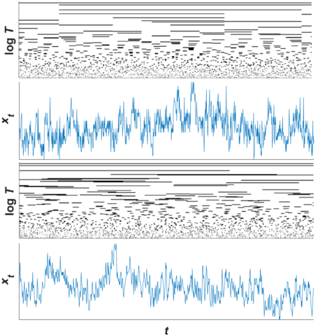
In the top half of the figure, one can see smaller unit intervals repeatedly nested within larger unit intervals across timescales to form hierarchical structures. The structures in this example are aperiodic because intervals are split at randomized points, but structures could instead be made periodic by splitting intervals at their midpoints instead. In the bottom half of the figure, the same unit intervals from above are shown with their phases randomized. Amplitude envelopes are created for nested and phase-randomized intervals by summing the values (all equal to one) of intervals present at each successive time point.
The nesting of structures is destroyed by phase randomization, which changes the resulting fluctuations in their amplitude envelopes. However, both envelopes converge on 1/f scaling because hierarchical temporal structure is preserved, as it does not capture information about specific clusters or nested structures. The same would be true for a periodic version of the model because 1/f scaling is also agnostic to periodicity – it essentially reflects the clustering of amplitudes (power) as a function of frequency.
This simple model creates “pure” hierarchical temporal structure that is devoid of the many other factors and influences that combine to create the richness of real speech and music signals. To distill hierarchical temporal structure from real signals, one can convert their amplitude envelopes into series of peaks defined only by their timing – a time series of zeros and ones that is called a point process (see Figure 20.2). Converting amplitude envelopes to point processes focuses analyses on temporal structure per se, and the threshold for identifying peaks can be set to achieve a specified overall rate of peaks that facilitates comparisons across recordings. The rate of peaks is a free parameter that is set to allow for a large dynamic range of peaks per unit time, so that hierarchical temporal clustering in the signal may be expressed as variability in the clustering of peaks. Peaks sometimes roughly correspond to glottal pulses, but they also correspond to aperiodic sounds of sufficient energy and generally any significant concentration of acoustic energy. Also, individual peaks are not intended to capture perceptual events (e.g., they may occur more rapidly than the auditory flicker fusion rate). Instead, clusters of peaks are the basic unit of analysis.
Illustration of Allan Factor analysis.
A speech example of hierarchical temporal structure is shown for the utterance “all we have to decide is what to do with the time that is given to us.” The acoustic waveform is at the bottom, the amplitude envelope in the middle, and peaks of the envelope above the threshold used for Allan Factor analysis. Brackets above show example windows over which peaks are counted and differenced over time to measure clustering. Window sizes roughly correspond to different overlapping linguistic timescales of prosodic temporal structure.
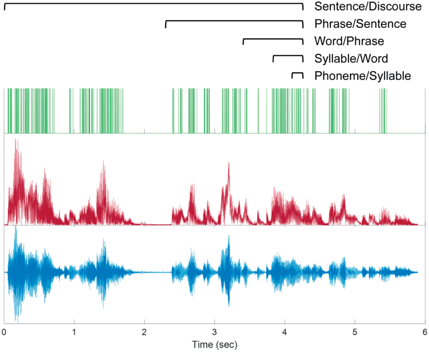
The resulting point processes are submitted to Allan Factor analysis, which quantifies the degree of clustering across the range of available timescales given the time series length and resolution, without identifying individual clusters at any given timescale. Hierarchical temporal structure is expressed in Allan Factor analysis as a positive relationship between timescale and average amount of clustering at that timescale, in logarithmic coordinates. The degree of hierarchical temporal structure can be measured by the logarithmic rate of increase in average clustering.
20.3 Hierarchical Temporal Structure in Speech
Allan Factor analysis has been applied to many hours of speech recordings from several different languages under a range of speaking conditions, including talks and other monologues, rapping, singing, infant-directed speech, computer-generated speech, and conversations in one and two languages (Alviar et al., Reference Alviar, Dale, Kello, Rogers, Rau, Zhu and Kalish2018; Falk and Kello, Reference Falk and Kello2017; Kello et al., Reference Kello, Bella, Médé and Balasubramaniam2017; Schneider et al., Reference Schneider, Ramirez-Aristizabal, Gavilan and Kello2020). The first and foremost result is that speech exhibits a characteristic pattern of hierarchical temporal structure that holds true in all cases, regardless of language spoken or idiosyncrasies of recording conditions.
The pattern is characterized by a relatively steep rise in average clustering as the Allan Factor function goes from timescales of tens of milliseconds to about one second, followed by a tapering in the rate of increase in clustering as timescales extend to tens of seconds (longer timescales require longer recordings of 10+ minutes that are difficult to find or collect). This general pattern of steep-then-tapering suggests that speech exhibits strong hierarchical structure for the timescales over which much of linguistic processing occurs – phonemes, syllables, words, phrases, and short sentences. Clustering subsides as sentences become longer and timescales stretch out to multiple sentences.
The pattern of tapered clustering at longer timescales may be partly due to the lengths of recordings being limited to around four–five minutes. Recordings were generally intended to contain uninterrupted speech signals throughout, which inhibits clustering at the longest timescales measured. Breaks in activity lasting tens of seconds are generally unwanted in audio recordings because there is an expectation of something being recorded. Such breaks may come about naturally under certain conditions, perhaps during casual or intimate conversation for example, but further work is needed to investigate.
While it is possible that tapered clustering may be partly due to recording conditions, results indicate that tapering also varies systematically across individuals, even when they are speaking different languages. Schneider et al. (Reference Schneider, Ramirez-Aristizabal, Gavilan and Kello2020) recorded pairs of Spanish-English bilingual speakers having conversations in the three different language conditions: Spanish, English, and a mixed condition in which one partner spoke Spanish while the other spoke English. Audio recordings were individual to each speaker, which allowed for within-speaker comparisons of hierarchical temporal structure when speaking the same language or different languages. Results showed that variations around the general steep-then-tapered pattern were highly correlated (mean B = 0.77) within speakers, regardless of whether correlations were within Spanish or English, or between the two languages.
These results show that hierarchical temporal structure, as measured by the adaptation of Allan Factor analysis, reflects the speaking style of individuals rather than the specific language or words being spoken. Consistent with this conclusion, Kello et al. (Reference Kello, Bella, Médé and Balasubramaniam2017) found that TED talks all had highly similar patterns of hierarchical temporal structure across seven different languages. When combined with the results from Schneider et al. (Reference Schneider, Ramirez-Aristizabal, Gavilan and Kello2020), the TED talk pattern seems to reflect the consistent style and manner in which TED talks are given. The pattern consists of a specific tilt and bend to the increase in clustering with timescale, which is difficult to interpret on its own. Next, recent studies are reviewed that begin to shed light on how to interpret systematic patterns and variability in hierarchical temporal structure.
20.4 Interpretable Variability in Hierarchical Temporal Structure
Abney et al. (Reference Abney, Paxton, Dale and Kello2014) reported the first study to employ Allan Factor analysis adapted for measuring hierarchical temporal structure in speech acoustics. They analyzed conversations from a study by Paxton and Dale (Reference Paxton and Dale2013) in which pairs of individuals engaged in either affiliative conversations (e.g., shared interests in entertainment) or argumentative conversations. The latter were created by pairing individuals who took opposing positions on “hot button” issues such as abortion based on a prior survey, and then instructing them to talk about the issue. The authors analyzed audio recordings of individual speakers as in Schneider et al. (Reference Schneider, Ramirez-Aristizabal, Gavilan and Kello2020), and results showed a similar steep-then-taper pattern, but there was greater hierarchical temporal structure in the longer timescales for conversations versus monologues such as TED talks. The reason is that conversations include more pauses for turn-taking and interacting, which creates clustering, whereas speaking is more continuous in monologues such as TED talks.
Abney et al. (Reference Abney, Paxton, Dale and Kello2014) also found more tapering for affiliative compared with argumentative conversations. This difference indicates that speakers can alter the degree of hierarchical temporal structure based on the mode of conversation. The authors conjectured that the argumentative conditions triggered more formal speech registers that, among other factors, caused speakers to enunciate more carefully and clearly compared with affiliative conversations in which speaking can be looser and more fluid. This conjecture is supported by the finding that hierarchical temporal structure changed in the prosodic timescales of hundreds of milliseconds and longer, rather than more fine-grained phonetic features that speakers may not be able to control. Since this first study, three other studies of speech under varying conditions have found similar effects that corroborate the original conjecture.
First, Kello et al. (Reference Kello, Bella, Médé and Balasubramaniam2017) compared hierarchical temporal structure measured in original TED talk recordings with those created by Google speech synthesis when reading transcripts of the talks. Allan Factor analysis showed that prosodic timescales for synthesized speech were devoid of temporal structure compared with original recordings, in that the Allan Factor function tapered off to a flat line. Given that the same words were spoken in both conditions, this result can be attributed to the failure of speech synthesis (at the time) to use prosody as a channel for communicating meaning and emotion.
Second, Ramirez-Aristizabal et al. (Reference Ramirez-Aristizabal, Médé and Kello2018) found that hierarchical temporal structure in prosodic timescales (and not the faster phonetic timescales) is more tapered for fast versus slow rates of speech. They instructed participants to read off a teleprompter excerpt from a speech by Barack Obama. The speed of the teleprompter was manipulated to be either slower or faster than the pace of the original speech to induce relatively slow versus fast speaking. Also, the original recording of Obama giving the speech was slowed down or sped up using an algorithm for manipulating speech rate without affecting pitch so that the result is relatively natural sounding. For both the algorithm and the teleprompter, tapering was less pronounced for slow speaking and more pronounced for fast speaking. Changing the pace of speaking has several effects of prosody (Jun, Reference Jun2003), but giving a slow and deliberate speech entails greater enunciation compared with “cutting corners” to get through a hasty speech. Indeed, hastened speech is more likely to sound flat, akin to a computerized voice.
Third, Falk and Kello (Reference Falk and Kello2017) analyzed hierarchical temporal structure in recordings of mothers singing a song or telling a story in German to either their infants or adult confederates. Singing or speaking to their infants induced infant-directed speech, whereas doing the same for adults induced adult-directed speech. As one might expect given the prior two studies, hierarchical temporal structure was more pronounced in prosodic timescales (and again not the faster phonetic timescales) for infant-directed versus adult-directed speech (also see Chapter 38). The authors interpreted this result as indicating that mothers exaggerated prosodic information for their infants. Convergent evidence for purposeful exaggeration also came from Boorom et al. (Reference Boorom, Alviar and Zhang2022) who found that adult speech directed at children diagnosed with autism spectrum disorder had greater hierarchical temporal structure compared with typically developing controls. In both cases, exaggeration may serve to grab the child’s attention, and it could also serve to aid speech development and comprehension.
The latter possibility leads to the hypothesis that hierarchical temporal structure may vary as a function of the degree of prosodic composition – that is, the presence and distinctiveness of prosodic boundaries and units as expressed in the speech signal. As with prosody in general, hierarchical temporal structure is hypothesized to carry information about meaning, intention, emotion, mode of interaction, and other possible channels of communication and coordination. On this hypothesis, tapering in hierarchical temporal structure occurs when these layers are less composed.
As a further test of the composition hypothesis, Kello et al. (Reference Kello, Bella, Médé and Balasubramaniam2017) tested whether different kinds of music might also vary in their degree of layering of temporal structure. The authors applied the same Allan Factor method of analysis to four different categories of music – contemporary pop, rap, jazz improvisation, and classical symphonies. The composition hypothesis predicts that symphonies should have the greatest degree of nested clustering because composers explicitly add layers of structure for each of the instruments. Results bore out the prediction, in that nested clustering increased steadily across all measured timescales, as in 1/f scaling, but only for classical music. By contrast, rap and popular music had bends in their Allan Factor functions that reflected their beat structure. More interestingly, jazz showed a degree of tapering in the longer timescales that was remarkably similar to the tapering for recordings of conversations. Jazz improvisation has been likened to a conversation among musicians (Sawyer, Reference Sawyer, Miell, MacDonald and Hargreaves2005), but heretofore there was little if any quantitative evidence for the comparison. The Allan Factor results support an underlying connection between prosody and music hypothesized in previous studies (Patel et al., Reference Patel, Peretz, Tramo and Labreque1998).
20.5 Conclusions
This chapter reviewed a growing body of evidence that speakers can control the rate of growth of temporal structure with timescales, referred to as the degree of hierarchical temporal structure. Evidence indicates that this control governs the amount of prosodic structure and composition in speech, possibly through a relative sharpening or blurring of prosodic units and boundaries. Studies show that the degree of hierarchical temporal structure reflects the difference between more hastened versus measured rates of speech (Ramirez-Aristizabal et al., Reference Ramirez-Aristizabal, Médé and Kello2018), more informal versus formal speech registers (Abney et al., Reference Abney, Paxton, Dale and Kello2014), adult-directed versus infant-directed speech (Falk and Kello, Reference Falk and Kello2017), and monologues versus dialogues (Kello et al., Reference Kello, Bella, Médé and Balasubramaniam2017).
A similar control parameter also appears in analyses of musical recordings in which the more layered compositions of classical music have greater degrees of hierarchical temporal structure compared with contemporary popular music and other less layered forms of music (Kello et al., Reference Kello, Bella, Médé and Balasubramaniam2017). Taken together, these studies suggest that listeners can distinguish degrees of hierarchical temporal structure, and speakers may vary this control parameter to signal different modes of communication to interlocutors (Alviar et al., Reference Alviar, Dale, Dewitt and Kello2020), and aid speech development and comprehension (Abney et al., Reference Abney, Warlaumont, Oller, Wallot and Kello2017; Boorom et al., Reference Boorom, Alviar and Zhang2022).
Hierarchical temporal structure such as classical music has been found in recordings of thunderstorms as well, and Allan Factor functions for human conversations were like those for improvisational jazz as well as vocalizations of killer whales communicating in groups. These results indicate that prosodic and hierarchical temporal structure can be composed by people, animals, or natural causes (Ravignani et al., Reference Ravignani, Dalla Bella and Falk2019). Hierarchical temporal structure serves to situate prosodic composition and structure in the broader context of language, music, and vocal communication.
Summary
Prosody is defined over several layers of hierarchical temporal structure. A growing number of studies indicate that variations in prosodic information correspond to variations in temporal clustering of acoustic energy as a function of timescale. Speakers can control hierarchical temporal structure in prosodic timescales for various reasons, including who is being addressed and under what circumstances.
Implications
Prosodic structure is sometimes considered as periodic, and linguistic hierarchies are often represented in terms of nested structures, but hierarchical temporal structure in the range of prosodic timescales may also be aperiodic and not necessarily nested.
Gains
Studies of hierarchical temporal structure may help to link prosody with music, animal vocalizations, and other temporal structures in nature such as 1/f scaling. They may also illuminate mechanisms of control in communication and provide a broad basis for linking measures of cortical activity with speech activity.
21.1 Introduction
Rhythm in speech is the temporal structure created by patterns of variation in duration, fundamental frequency (f0), and intensity. These patterns can result from articulatory processes (Tilsen, Reference Tilsen2019), characteristics of the spoken language (Cutler et al., Reference Cutler, Dahan and Van Donselaar1997), and pressures arising from comprehension processes (see Chapters 18 and 19). The rhythmic patterns in naturally produced speech vary both within and between speakers.
In instances where we wish to control or manipulate speech prosody, this natural variation presents a challenge. For example, if contrasting the effect of different intonational contours on speech perception, it would be necessary to ensure that non-temporal parameters (f0, intensity, phonation type) are not correlated with temporal patterns that could offer an alternative interpretation of effects. Conversely, if contrasting different temporal patterns, it would be necessary to ensure that the independent variable is not confounded by non-temporal parameters.
Faced with this type of challenge, there are four options: to record speech produced by a trained phonetician, to synthesise speech, to alter the timing of a speech recording (retiming), or some combination of these (e.g., the retiming and resynthesis of speech produced by a trained phonetician in Smith and Rathcke, Reference Smith and Rathcke2017). Speech produced by a phonetician or by speech synthesis are both valuable tools for research. However, even trained phoneticians may not be able to control timing very precisely, whereas controlling timing in synthetic speech requires a priori decisions to be made in the parametrisation of the tool. In contrast, retiming speech can produce multiple signals with different temporal characteristics from a single source.
Although it would be preferable to avoid signal degradation or disruption of local prosody, there are ways of mitigating the impact. One approach is to counterbalance these effects across experimental conditions. For example, when producing isochronous stimulus items, Aubanel et al. (Reference Aubanel, Davis and Kim2016) created a matched anisochronous condition with the same amount of absolute temporal distortion. While this allows for comparisons between different retimings, it does not allow for naturalistic stimulus design. A further risk is that the experimental manipulation is more apparent to the participant.
Where it is a priority that stimuli sound natural, it is important to consider subtle differences in how a retiming might affect an utterance. Two important factors to this are the amount of disruption to the signal and the location of the disruption. The least disruptive retiming would be no retiming at all, with the most disruptive retimings approaching the hypothetical physical limits of the transformation where parts of the signal are sped or slowed by infinite factors. Therefore, a possible approach is to perform the minimally disruptive retiming that achieves the desired temporal structure. However, extreme disruptions may have subtle effects in certain positions. For example, a part of a signal sped by an infinite factor would be equivalent to the removal of that part of the signal. In most cases this would be an unacceptable disruption to the signal. However, there would be special cases with ecologically valid interpretations, such as retiming a recording of the word LIBRARY produced as /laɪbrəri/ in a manner that results in the elision of the medial syllable to produce /laɪbri/, amounting to complete deletion of one or more segments, as observed for many phenomena cross-linguistically (e.g., Johnson, Reference Johnson, Yoneyama and Maekawa2004; Dilley and Pitt, Reference Dilley and Pitt2010; Bürki et al., Reference Bürki, Ernestus, Gendrot, Fougeron and Frauenfelder2011; Turnbull, Reference Turnbull2018). Similarly, infinite slowing of a section of the signal would be an extreme disruption, but at a word or syntactic boundary, it would be equivalent to a speaker taking a pause (Zellner, Reference Zellner and Keller1994; Kentner et al., Reference Kentner, Franz, Knoop and Menninghaus2023). These retimings may be subtle in the sense that they would not necessarily sound unusual, but if not applied with careful consideration of the prosodic context, they could result in unacceptable disruptions to the signal.
The aim of this chapter is to provide an overview of the possibilities available to researchers producing retimed stimuli. Three methods of producing retimed stimuli are presented and their utility is demonstrated by creating utterances to have an isochronous rhythm. It is expected that all three methods will enhance the periodicity of the utterances to match the frequency implied by the isochronous intervals. Following this, we present an example of how the last of these three methods may be generalised to produce a wider variety of stimulus types.
21.2 Isochronous Speech
21.2.1 Materials
A corpus composed of a male speaker of Scottish English producing simple mathematical sums was recorded and segmented into words for the purpose of demonstrating the three retiming methods. The corpus was composed of all 66 possible correct sums containing only the numbers from ONE to TEN, and the operators indicated by the words PLUS, MINUS, and IS, for example, FOUR PLUS FIVE IS NINE or THREE MINUS TWO IS ONE. All sums containing SEVEN were excluded, leaving MINUS (produced as /ˈmaɪnəs/) as the only polysyllabic word. Sums were spoken with a quasi-isochronous rhythm at an approximate rate of one word per second with short silences between words.
21.2.2 Retiming Methods
Three approaches to retiming speech are considered here. In each case the interval between perceptual centres (p-centres; Morton et al., Reference Morton, Marcus and Frankish1976; Chapter 11) is held constant at one second. Here, p-centres are defined as the maximum rate of change of the amplitude envelope for a syllable; however, these approaches could be applied to alternative definitions. The first method achieves isochronous retiming by increasing the rate of the entire utterance and extending or inserting silences. The second method alters the rate of the signal between p-centres, and the third method continuously varies the rate of the speech.
In order to compare these methods, we applied them to create stimuli with the shared specification that the p-centres of each word should be equally spaced to achieve an isochronous utterance. For this reason, the term anchor point is used here somewhat interchangeably with the term p-centre. However, these methods are not limited to producing isochronous stimuli. Any feature that can be annotated as a fixed point could be used if there is a motivation to control the timing of the associated event.
Isochrony has advantages for the purposes of evaluation. The effectiveness of the retiming technique can be measured by the extent to which the signal is made more isochronous. Isochrony is defined in the time domain as a signal with equal time intervals between events and can be measured using autocorrelation.Footnote 1 Furthermore, isochrony would also be expected to be observable in the frequency domain as the rate of intervals per unit time. This can be measured using discrete Fourier transformation (DFT). Typically, the DFT representation will show a high level of spectral power at the frequency corresponding to the interval between events. There are, however, potential theoretical implications for the choice of measure. A DFT decomposes a signal into sinusoidal waves whether or not the signal is composed of sinusoidal waves. As a result, it may not be best suited to detect recurrences of irregular waveforms (Zhou et al., Reference Zhou, Melloni, Poeppel and Ding2016). For example, the amplitude envelope of an utterance with a regular one-second interval between syllables would typically have high spectral power at a frequency of 1 Hz. However, an irregular signal could have a high concentration of spectral power at 1 Hz because of a strong 1 Hz component to the signal such as a single cycle of a 1 Hz sinusoidal wave repeating at irregular intervals. In contrast, evaluating isochrony in the time domain using autocorrelation will capture recurrences even if no sinusoidal pattern is apparent in the amplitude envelope.
To provide a representation of the rhythmic structure of the input signals, the amplitude envelope was extracted using the extract_env function from the retimer package (Beith, Reference Beith2022). This function is an implementation of the vocalic envelope extraction method proposed by Tilsen and Johnson (Reference Tilsen and Johnson2008), with the additional option to control the low-pass filter and output sampling frequency. These modifications make it possible to extract a smoothed envelope by setting the sampling frequency higher than the low-pass filter frequency. Onsets were then detected by finding peaks in the rate of change in amplitude. An amplitude envelope of an example utterance is shown in the upper panel of Figure 21.1, annotated with the p-centres that are used as anchor points.
Retiming warp paths.
Upper panel (A) shows the amplitude envelope of the input signal annotated with p-centre estimates.
Lower panel (B) shows the mapping of each of the three retimings (left axes) to the input signal (bottom axes).
All retimings were performed in R with the wsola function from the retimer package. This function is a translation of the wave-similarity overlap-and-add algorithm (WSOLA) implemented in the TSM (time-scale modification) toolbox (Driedger and Müller, Reference Driedger and Müller2014) for Matlab. A translation for Python users is also available in the PyTSMod library (PyTSMod, 2022). Like OLA, WSOLA involves overlapping windowed slices of the signal to compress or extend the duration of a part of the signal. The advantage of WSOLA is that it allows the positioning of the overlaps to be adjusted to minimise phase discontinuity. The techniques discussed here could also be applied to any retiming algorithm implemented in either the TSM toolbox or PyTSMod. Additionally, an OLA transformation can also be produced by using the WSOLA with the tolerance parameter set to 0 (Driedger and Müller, Reference Driedger and Müller2014). Many speech researchers will also be familiar with time-domain pitch-synchronous overlap-and-add (TD-PSOLA; Valbret et al., Reference Valbret, Moulines and Tubach1992) due to its implementation in Praat (Boersma and Weenink, Reference Boersma and Weenink2023). This method performs a source-filter decomposition, which makes it additionally useful for pitch transformations, but still shares the limitations of OLA in terms of phase discontinuities.
21.2.2.1 Method 1: Serialisation
Most simply, what is referred to here as serialisation is an utterance that is created by presenting individual words in a sequence. This is the same stimulus presentation method that led to the observation that an utterance created with regularly spaced word onsets does not result in a perceptually regular utterance (Morton et al., Reference Morton, Marcus and Frankish1976). It is also an auditory analogue to the common rapid serial visual presentation paradigm (RSVP; Potter, Reference Potter1984).
Despite the intuitive appeal of this method, the actual process of producing stimulus items can be challenging. Altering the temporal position of a word in a continuous utterance without silences at word boundaries will result in an overlap with one of the neighbouring words. Therefore, to prevent overlaps, either the rate of words must be increased to shorten their durations or the length of the utterance must be increased to provide additional space.
The implementation presented here is constrained by the previously mentioned requirement that the p-centres of each word are equally spaced by a fixed interval of one second. The function used here is provided in the retimer package (Beith, Reference Beith2022) as get_serial_anchors(). It takes two sets of anchor points in seconds – corresponding to the original p-centres and desired p-centres – as arguments, along with the onsets and offsets of the words. This assumes that there is silence between words in the original utterance or that the researcher has inserted silences prior to the transformation. The function calculates the minimum reduction in speech rate that will prevent overlaps and returns a set of anchor points corresponding to word onsets and offsets that will result in the desired p-centre alignment. If a sample rate is provided, these anchors are transformed to index time in samples rather than seconds. A retiming factor can also be provided if – as is the case here – all items are to be retimed by a common factor. The resulting anchor points, along with the input signal and sample rate, can then be passed to the wsola function to return the retimed signal.
An alternative approach would be to use the anchor points returned by get_serial_anchors() or an equivalent calculation to individually present words or concatenate signals with silence. Presenting individual words may be more appropriate when generating stimuli in real time during an experiment. However, concatenation may also require the insertion of spectrally matched noise rather than silences.
21.2.2.2 Method 2: Point to Point
A logical progression from method 1 would be to relax the constraint that the rate increase applied to each word is uniform across words. However, the benefits of this approach would be limited as the necessary rate increase to prevent overlaps would be constrained by the position of neighbouring words. Therefore, it would still be necessary to insert silence in most cases. A solution to this is to annotate the utterance from p-centre to p-centre and apply the retiming to these intervals.
One of the advantages of this method over method 1 is that there is no need to rely on heuristics to calculate anchors without overlaps. The researcher is required only to provide a list of anchors referring to the p-centres in the input signal and a list of anchors referring to the desired timing of the p-centres in the output signal.
As this method does not insert any silence, or change overall utterance duration, there is no change to the average rate of the utterance. Instead, sections that are sped are compensated for by sections that are slowed. Additionally, the durations of pauses between words are preserved relative to the surrounding context. The cost of this is that tempo can change within a word and phone as p-centres are not typically located at word or even phone boundaries. This discontinuity in the speech rate will be most pronounced when the speech rate in the source recording alternates between fast and slow, as this would result in one part of the word being sped and another part slowed.
21.2.2.3 Method 3: Continuous
In the first method there was a discontinuity in time as silences interrupted the speech. In the second method there was a discontinuity in rate as fast intervals followed slow and slow followed fast. Method 3 smooths the transitions at rate changes by continuously altering the speech rate.
A convenient way of achieving this is to interpolate a spline passing through the same anchor points as would be used in the prior method. A spline provides a smooth, continuous function between anchor points so that abrupt discontinuities are avoided. In some cases, fitting a spline could result in a set of anchors that would imply that parts of the signal were to be reversed. This can be avoided by using the spline algorithm proposed by Hyman (Reference Hyman1983) that fits a cubic spline to a series of points while preserving the monotonicity of the input. This algorithm is available as the spline function in R and through the SciPy (Virtanen et al., Reference Virtanen, Gommers and Oliphant2020) library for Python.
21.2.3 Analysis
Each of these three retiming methods will result in the desired p-centre onset time. However, they do so with different degrees of temporal distortion and with differences in the distribution of these distortions over the duration of the utterance.
Retimings can be visualised by plotting the warp path of the original and retimed speech. The warp path is given by the intersection of matched points projected from adjacent axes, as shown in the lower panel of Figure 21.1.
The first method results in a warp path made up of two types of lines: the diagonal segments that are all projected at a common angle corresponding to the retiming factor, and the vertical segments corresponding to insertions of silence. This is indicative of a discontinuity in the speech itself. In contrast, the warp path resulting from method 2 is exclusively made up of diagonal segments with different slopes. While continuity of speech content is preserved, there are discontinuities in the speech rate at each of the anchor points annotated with dotted lines in Figure 21.1. Method 3 is made up of continuously changing slopes, while achieving a similar overall path to method 2.
Three retimed utterances, one using each of the three methods, were created for each of the 66 sums. They were evaluated in terms of the disruption to the signal and their effectiveness in producing isochronous stimuli. The full set of stimulus examples and a vignette of one example is available in the supplementary repository (Beith et al., Reference Beith, Barr and Smith2024).
21.2.3.1 Temporal Distortion
The distinctions between different realisations of isochronous retimings are not merely conceptual. The warp path represents disruptions to the original signal, with the least disruptive path being the shortest path – a diagonal line of fixed slope – representing an unaltered signal. The least disruptive retiming would be the shortest path that passes through each of the anchor points. By definition, this is method 2 as each segment of the path is the shortest path between sequential pairs of anchor points.
Temporal distortion was measured by calculating the additional length of the warp path. In order to normalise the path length measure, and not to favour shorter items or penalise longer items, anchor points were first scaled between 0 and 1. This makes  the shortest possible warp path length between the input and output signal. There is also a theoretical upper limit of 2, which would correspond to a path made entirely of vertical and horizontal steps. As these limits are known, the path length is expressed here as a cost over and above the shortest possible path, and additionally scaled so that a warp path of length
  would have a cost of 0 and a warp path of length
  would have a cost of 1.
The results of the warp path cost analysis are shown in Table 21.1. They show a distinction between the similarly short paths of methods 2 and 3 and the longer path of method 1. Here, there appears to be a small advantage to the point-to-point retiming compared to the continuous method when looking at the median. A larger difference between these methods is seen at the upper bound of the 95% highest density continuous interval (HDCI).
Values show lengths of warp path over and above the shortest possible path and scaled to show the hypothetical limit as 1. Lower and upper bounds of 95% highest HDCI are shown.
| 95% HDCI | |||
|---|---|---|---|
| Method | Median | Lower | Upper |
| 1: Serialisation | 0.057 | 0.009 | 0.207 |
| 2: Point to point | 0.007 | 0.000 | 0.085 |
| 3: Continuous | 0.008 | 0.000 | 0.176 |
21.2.3.2 Increased Isochrony
In order to validate the retiming methods presented here, the increase in isochrony was measured in both the time domain and the frequency domain. This was achieved using the same item set as for the previous warp path length measure. An additional control condition was included as a reference. For the control condition, the average interval between syllables was calculated and the utterance was sped or slowed to have the same average interval duration as the isochronous stimuli. This condition would have a normalised path length of  , or a path length cost of 0 for all items. It was expected that all three retiming methods would have increased spectral power at the retimed frequency of 1 Hz, and increased autocorrelation at the retimed period of one second. Additionally, retimed signals would be expected to increase autocorrelation at multiples of the retimed period.
The FFT (fast Fourier transformation) method used here was adapted from Tilsen and Johnson (Reference Tilsen and Johnson2008). A vocalic amplitude envelope was extracted using the function extract_env in the retimer package. While Tilsen and Johnson (Reference Tilsen and Johnson2008) suggest low-passing the signal at 80 Hz and then also downsampling the signal to 80 Hz, here the signal was low-passed at 32 Hz and downsampled to 1,024 Hz. The lower low-pass frequency smooths out more high-frequency information, and the higher sample rate provides a higher resolution in the FFT. Setting these values to powers of 2 ensured that the FFT of the signal would have frequency bins at whole numbers, and crucially the 1 Hz bin of interest. The same amplitude envelope was used for the autocorrelation function (ACF) analysis. For both analyses, the spectra were averaged across all items.
Results of these analyses are shown in Figure 21.2. The gain in spectral power shown in the upper panel at 1 Hz appears modest for all three conditions with a small advantage for the latter two, less destructive, methods. The frequency spectrum also shows peaks for all three retimings at harmonic frequencies of 2, 3, and 4 Hz. The difference between control and retimings is more apparent in the autocorrelation analysis shown in the lower panel. Here, there may be a slight advantage to the first method.Footnote 2
Periodicity and recurrence spectra.
Left: FFT and ACF spectra of the original amplitude envelope and amplitude envelopes resulting from each of the three retimings. Ribbons indicate +/− 1.96 SE. Right: View of only the 1 Hz and one-second peak heights with error bars showing the same confidence interval as ribbons.
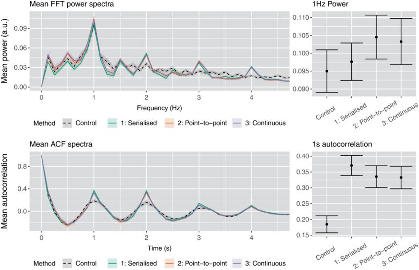
Figure 21.2 Long description
Top: A line graph of mean power versus frequency. It plots overlapping and fluctuating lines for control, serialized, point to point and continuous. The lines show peaks at 1, 2, 3, and 4 Hertz. To its right, an error bar graph plots the mean power, which are as follows. Control, 0.095. Serialized, 0.097. Point to Point, 0.105. Continuous, 0.103. Bottom. A line graph of mean autocorrelation versus time. It plots overlapping and fluctuating lines for control, serialized, point to point, and continuous. The lines show peaks at 1, 2, 3, and 4 seconds. To its right, an error bar graph plots the mean power, which are as follows. Control, 0.17. Serialized, 0.037. Point to Point, 0.33. Continuous, 0.33. The values are estimated.
21.2.4 Discussion
Depending on the hypothesis being investigated, the definition of isochrony may vary. For example, if the researcher hypothesises that the oscillatory structure of the amplitude envelope will elicit neural entrainment, it would be preferable to demonstrate a cyclical periodic structure in the stimulus. Alternatively, if it was hypothesised that greater regularity of edges in the amplitude envelope would increase the salience of the rhythmic structure, recurrence might be more important than cyclical periodicity.
Method 1 appears to be less appropriate for increasing periodicity. Due to the insertion of silence, any naturally occurring cyclical pattern could be disrupted by the creation of discontinuities. Furthermore, as the speech rate is increased without reducing the duration of the utterance, any existing periodicity in the envelope would no longer be coherent with the imposed frequency. This may explain the more modest power increase shown in the close-up view of the 1 Hz bin in the upper right of Figure 21.2. For all retimings, power is also increased at the harmonic bins (2, 3, and 4 Hz), as would be expected from a periodic signal, with no evidence of recurrences at time-domain equivalences (0.5, 0.25, or 0.125s) in the ACF spectrum. This again highlights that power at a frequency in an FFT does not necessarily correspond to recurrence at that frequency. In contrast, there appears to be an advantage to the first method over the others in the ACF measure. This may be because all words were increased by the same rate and, therefore, regularities in the original production of the words were retained.
The advantage of methods 2 and 3 in the FFT analysis may not be enough to justify their selection over method 1. Similarly, their disadvantage compared to method 1 in the ACF analysis may not be enough to justify selection of method 1. The clearer difference is apparent in the warp path cost measure. Both of these measures have lower median values than the lower bound of the 95% HDCI for method 1. This is unsurprising, particularly in the case of method 2, as it defines the shortest path passing through the required anchors. The additional cost of the third method appears to be minimal except with a higher upper bound. This would suggest that more careful checking of outliers may be required.
The results presented here may not necessarily generalise to other stimulus sets. Consider that neither point-to-point nor continuous retiming methods would alter an already isochronous stimulus item, while the serialisation method would insert silences. By extension, the measures reported here capture not only the performance of the retiming method but also the irregularity of speech in the source recording.
21.3 Rhythmic Chimeras
The flexibility of continuous retiming demonstrated in method 3 makes it useful for many applications beyond creating isochronous speech. In natural speech the temporal structure varies in subtle ways that would be challenging to define a priori. Two utterances could consist of the same sequence of words and phrase structure, but the rhythmic structure may vary between speakers or settings.
This section shows how continuous retiming can be used to create a rhythmic chimera. The analogy of a chimera is borrowed here from the term auditory chimera used by Smith et al. (Reference Smith, Delgutte and Oxenham2002) to refer to combining the fine detail of one auditory signal with the amplitude envelope of another to create a hybrid of the two. Here, the rhythmic chimera does not replace the amplitude envelope but instead uses it as a reference to warp the rhythmic structure of one utterance to that of another.
21.3.1 Materials
Example utterances were taken from the CHAINS corpus (Cummins et al., Reference Cummins, Grimaldi, Leonard and Simko2006). This corpus was created to support speaker identification research and consists of 36 speakers producing a range of sentences and longer texts under different reading conditions. Here, the solo sentence tasks were used where the speakers read the sentences at their own pace. Recordings of a male and a female speaker, each producing the same sentence, were sampled from these sentences to demonstrate the creation of rhythmic chimeras.
21.3.2 Method
There are three steps to the creation of a rhythmic chimera. These are feature extraction, alignment, and retiming. A vignette of the full stimulus creation process using R is provided in the supplementary repository (Beith et al., Reference Beith, Barr and Smith2024).
21.3.2.1 Feature Extraction
The first step is to produce time series of each of the signals. The simplest option would be to use the amplitude envelope as with the previous examples. However, an improved alignment can be achieved by using a multivariate signal.
Mel-frequency cepstral coefficients (MFCCs) have been used to perform alignments of utterances in previous studies (e.g., Cummins, Reference Cummins2009) and are used extensively in automatic speech recognition (ASR) tools (e.g., Young et al., Reference Young, Evermann and Gales2015; McAuliffe et al., Reference McAuliffe, Socolof, Mihuc, Wagner and Sonderegger2017). The advantage of MFCCs is that they reduce the feature representation from a full spectrogram to a smaller number (12 in the examples mentioned) of dimensions. More recent ASR tools such as OpenAI’s Whisper (Aldarmaki et al., Reference Aldarmaki, Ullah, Ram and Zaki2022) use full mel-spectrograms. Following this approach, mel-spectrograms with 80 bins and 10 ms time steps (i.e., 100 Hz sampling frequency) were used for feature extraction. As the mel-spectrogram is an intermediate step of MFCC extraction, the melfcc function from the tuneR package (Ligges et al., Reference Ligges, Krey, Mersmann and Schnackenberg2023) was adapted for this purpose.
21.3.2.2 Alignment
Following feature extraction, alignment was performed by dynamic time warping (DTW) using the dtw package (Giorgino, Reference Giorgino2009). The warp paths shown in Figure 21.1 are similar to those that would be obtained from a DTW analysis. Each point in one time series refers to a matched point in the other time series. For DTW, this is done by finding the optimal path through the distance matrix of two signals that meets the defined parameters. When using a multivariate signal such as an MFCC or a mel-spectrogram, the distance method must be specified as “Manhattan.”
As demonstrated by the retiming methods in this chapter, there are many warp paths that can produce similar results. In DTW, paths can be subjected to local constraints to specify particular characteristics. As the intention here is to use the alignment to perform a retiming of the signal, the alignment should be usable as anchor points, preferably with minimal additional processing. Therefore, the alignment path between the two signals must be monotonically increasing.
This constraint can be achieved by specifying a step pattern. An extensive review of step pattern options is included in Rabiner and Juang (Reference Rabiner and Juang1993), and further documentation of options is available in the companion paper for the dtw package (Giorgino, Reference Giorgino2009). Although all step patterns are monotonically non-decreasing, many patterns, as with the serialisation approach (method 1), allow sequential points in one signal to be mapped to the same points in the other signal. Effectively, this would require the insertion of silence or the omission of part of the signal to implement. The Rabiner–Juang Type III step pattern (Rabiner and Juang, Reference Rabiner and Juang1993, Section 4.7) was used here to produce a monotonically increasing alignment. With this pattern, each step taken in one time series must correspond to one or two steps in the other time series.
21.3.2.3 Retiming
The alignment maps points in the mel-spectrogram of one signal to the corresponding points in the mel-spectrogram of the other signal. Therefore, the only step required to produce anchor points for a retiming is to rescale the alignment to the sampling frequency of the signal. Simply reversing the anchors allows for the retiming to be performed in the opposite direction.
This retiming would be useful if the intention was to retime one speaker to have the rhythmic structure of another. A further possibility is to produce ambiguous rhythmic chimeras. This can be done by averaging the anchor points to create a series of anchors representing the midpoint between the time a sound occurs in one speaker’s utterance and the time it occurs in the other speaker’s utterance. For example, if speaker A produces a sound at the time of 500 ms and speaker B produces that same sound at 1,000 ms, both recordings could be altered so that both speakers produce the same sound at 750 ms. The same principle could be extended to produce a continuum of rhythmic structures by weighting the averages.
The vignette provides examples of unaltered recordings of the two speakers and all combinations of full rhythmic chimeras and half-warped rhythmic chimeras. A final example places the two half-warped rhythmic chimeras in left and right channels of a stereo audio file to allow for aural inspection of the alignments.
21.3.3 Results
Rhythmic chimeras are achieved by using DTW both as a means of analysis and of producing the stimulus. Therefore, insofar as DTW is an appropriate means of analysis, the retiming is perfect. Furthermore, criticisms of the retiming could be addressed by altering the parameters (most likely the step pattern) of the DTW analysis.
The primary limitation is that more extreme differences between speakers’ rhythms will result in more disruption in the retimed signal. Where suitable to the experimental paradigm, the half-warped retiming presented here would be an appropriate method of minimising disruption. A further option would be to add additional constraints to the DTW step pattern. In the examples, type “a” slope weighting was used, incurring no additional cost for steps with steeper or shallower slopes. However, weighted slopes could be used to prefer unwarped steps at the local level over steeper or shallower slopes that provide a better fit. A global constraint can also be applied via a windowing function to prevent large deviations from the original signal.
21.4 Discussion
This chapter set out to demonstrate three methods available to researchers for producing stimulus items where temporal structure needs to be controlled or manipulated. To the extent that they were able to produce isochronous speech, all three methods performed well. By design, they ensured that the timing of the p-centre estimate occurred at the intended time. This was demonstrated by increased autocorrelation at the intended period in the time domain (ACF) analysis. When measured in the frequency domain (FFT), the increase in periodicity was less apparent, but with a potential benefit of point-to-point and continuous retiming over control and serialisation.
A limitation of the isochronous stimulus examples is that the speech used was initially produced with quasi-isochronous rhythm and with silences between words. It should not be assumed that these results would generalise to connected speech where a weaker relationship between periodicity in the amplitude envelope and syllable rate would be expected (Zhang et al., Reference Zhang, Zou and Ding2023). In these cases, segmentation will be more challenging and the effects of retiming methods should be assessed for suitability. Furthermore, as found by Aubanel et al. (Reference Aubanel, Davis and Kim2016), imposing strict regularity on speech with complex temporal structure can reduce intelligibility.
There are certain constraints that cannot be changed when altering the temporal structure of speech. Most crucially, information in the speech signal increases monotonically over time, and any transformation would be expected to be monotonically non-decreasing at a minimum. Or, more simply, it is unlikely that a researcher would want any part of the speech to be played backwards. The serialisation method for producing isochronous speech exemplifies one extreme of this limit, where silences are inserted reducing the rate at which the signal progresses to zero. In contrast, the point-to-point method minimises deviation from the rate of the source signal to produce the most efficient path that passes through the desired points. Finally, the continuous retiming method attempts to smooth transitions at rate changes.
For the purposes of this chapter, it is assumed that minimising disruption of temporal structure will in turn minimise disruption of existing prosodic structure. This is reflected in the choice of quantitative measures used to operationalise prosodic disruption. However, future research could benefit from expanding this scope to include qualitative and perceptual measures of prosodic structure.
A potential disadvantage of expressing these methods as warp paths is that it obfuscates some of the more intuitive differences. An equivalence of method 1 could be achieved by simply presenting individual words at predefined times. When constructing a stimulus item in this way, there may be no expectation that the item will sound like a natural utterance or even that it should have the grammatical structure of a sentence or phrase. There are cases where stimuli of this type will have value, such as the design adopted by Quené and Port (Reference Quené and Port2005) where effects of different timings of word presentation were compared. However, caution should be exercised if there is any intention to interpret findings as being generalisable to spontaneous connected speech (see Alexandrou et al., Reference Alexandrou, Saarinen, Kujala and Salmelin2020, for discussion).
Choosing to focus on the commonalities of each of the three retiming methods highlights the complementary relationship between retiming and DTW. While retiming is used for performing manipulations and DTW is used for analysis, both techniques can be expressed as a warp path. An accurate DTW analysis of a source signal and its retiming will result in a warp path resembling the anchor points used to perform the retiming. The steps allowed within these paths allow the researcher to meet the specific needs of their study.
In the case of an a priori temporal structure, such as the imposition of isochrony, the warp path maps a limited set of predefined anchors. Nonetheless, each of the three methods demonstrated had different local continuity constraints. In method 1 the angle could be either a diagonal of a fixed slope or vertical. In method 2 the angle of the slope could change, but only at fixed points. In method 3 the angle of the slope could change but the local change in angle was constrained by the effect it would have on the surrounding points. Recognising this relationship between retiming and DTW provides the stimulus designer with valuable insights from the DTW and speech recognition literature.
While isochrony provides a useful example, a researcher may not always be able to explicitly define the desired anchors in this way. Rhythmic chimeras provide an example of a more flexible approach to retiming a signal. In the example provided, a rhythmic chimera can be used to present one speaker’s utterance with another speaker’s temporal structure. This does not require the researcher to define the temporal structure a priori in terms of onsets or boundaries, yet it allows for a meaningful retiming.
Thus, the approach is valuable for exploring the contribution of temporal organisation to recognition of individual voices (Kello, Reference Kello2003) and accents (Mareüil and Vieru-Dimulescu, Reference Mareüil and Vieru-Dimulescu2006; Kolly et al., Reference Kolly, De Mareüil, Leemann and Dellwo2017; Smith and Rathcke, Reference Smith and Rathcke2017). Furthermore, the half-warped rhythmic chimera would have applications in experimental control of items. Multiple speakers with different voice qualities or realisations of segments could be presented as stimulus items with the same temporal structure. Overall, DTW-based methods offer a flexible and practical way to apply the temporal organisation of one utterance to the spectral structure of another, such as in situations where researchers want to explore how temporal cues yield different structural interpretations of the same phonemic content (e.g., different locations of word, morpheme, or prosodic boundaries; Smith and Hawkins, Reference Smith and Hawkins2012; White et al., Reference White, Mattys, Stefansdottir and Jones2015) or where the contribution of speech rate to the perception of segmental, lexical, or larger units is to be explored (e.g., Dilley and Pitt, Reference Dilley and Pitt2010; Reinisch et al., Reference Reinisch, Jesse and McQueen2011). The methods do so without requiring a priori linguistic assumptions, and allowing for straightforward generation of intermediate values, and their advantages in terms of convenience and naturalness can be explored in future research.
21.5 Conclusion
Retiming speech is a convenient and powerful way of investigating effects of rhythm. However, these manipulations degrade and distort the source signal, with the method chosen to perform the retiming impacting on the naturalness of the resulting stimuli. DTW provides an analytical framework to describe the properties of different approaches to retiming. Recognition of this complementary relationship gives the experimenter a greater ability to parametrise stimulus design to meet specific needs of the experiment. In doing so, this opens up new avenues for experimental stimulus creation that could investigate questions about the contribution of temporal structure to speech perception.
Summary
This chapter presents three methods of creating retimed stimuli with specific temporal characteristics. These methods are discussed in terms of how they affect the existing temporal structure of the speech signal. A further example is provided to highlight the versatility of retiming as a stimulus creation technique.
Implications
In bringing together a range of possible approaches to retiming speech, we hope to encourage researchers to think critically about the choices they make when designing speech stimuli with temporal manipulations. Rather than inventing new techniques, we have combined existing, well-documented tools in a way that highlights the available possibilities.
Gains
The methods presented in this chapter have the potential to be applied in a wide range of disciplines. Furthermore, by building on existing open-source tools, researchers and research software engineers can adapt these methods to meet the requirements of a wide range of paradigms.
22.1 Introduction
Linguistic rhythm is classically viewed as the binary alternation of stressed and unstressed syllables. Selkirk (Reference Selkirk1984) calls this the principle of rhythmic alternation (PRA), which arises in trochaic languages, such as German or English, from the underlying trochaic structure of the lexicon (see also Sweet, Reference Sweet1876; Féry, Reference Féry1998). (1) shows an example of alternation of stressed and unstressed syllables.
(1) Péter wóllte héute láufen.
Peter wanted today (to) run.
“Peter wanted to run today.”
In the present chapter it will be argued that a balance measure is better suited than binary alternation to formalize speech rhythm since multiple violations naturally occur in everyday speech as a result of the clustering of stressed or unstressed syllables. The juxtaposition of two or more stressed syllables produces a stress clash, whereas the clash of two or more unstressed syllables produces a stress lapse (Selkirk, Reference Selkirk1984; Hayes, Reference Hayes1995). Correspondingly, *LAPSE denotes a constraint according to which more than one unstressed syllable in the sequence is to be avoided. *CLASH denotes a constraint that a sequence of more than one stressed syllable is to be avoided. The example in (2) shows a sentence with three stress lapses (the relevant syllables are underlined).
(2) Róbert ságte, dass Nádja ihn bekláuen sóllte.
Robert said that Nadja him steal (from) should.
“Robert said that Nadja should steal from him.”
While no system currently exists to formalize the rhythmicity of an entire sentence, Shih et al. (Reference Shih, Grafmiller, Futrell, Bresnan, Vogel and Vijver2015) propose a measure that makes formalization possible, at least for smaller phrases. Here, a 1 is subtracted from the number of unstressed syllables that line up between two stressed syllables (see 3a). (3b) symbolizes a rhythmic alternating structure, where stressed syllables are represented by X and unstressed syllables by x. (3c) shows a LAPSE and (3d) a CLASH. In the course of rhythmic alternation, the value should therefore approach 0, as in (3b). *LAPSE (3c) and *CLASH (3d) are treated as equivalent according to Shih et al. (Reference Shih, Grafmiller, Futrell, Bresnan, Vogel and Vijver2015). They are each given the value 1.
(3a) | Number of unstressed syllables between two stressed syllables -1|
(3b) x X x X x; |1-1| = 0
(3c) x X x x X x; |2-1| = 1
(3d) x XX x; |0-1| = 1
(3a–d) show that the rhythmic structure of sequences with two stressed syllables can be formalized quite well. However, if the number of stressed syllables increases to three or more, the measure operates only to a limited extent; that is, it only refers to the space between two stressed syllables without relating the values to one another in longer structures. Thus, it is not possible to systematically distinguish between (4a), (4b), and (4c), although (4a) apparently has a much more balanced rhythm than (4b) and (4c).
(4a) X xx X xx X xx X xx
(4b) X xxxx X x X X
(4c) X xxxx X x X xx X
The examples already suggest that the binary description of rhythm is not sufficient for more complex linguistic units. In (4a), for example, a dactylic rhythm is indeed shown, which, in addition to the trochee, may represent a rhythmic unit perceived as regular for everyday German (see, among others, Hanna, Reference Hanna2003; Vogel et al., Reference Vogel, van de Vijver, Kotz, Kutscher, Wagner, Vogel and Vijver2015). Therefore, the goal of this chapter is to develop a rhythmic measure that goes beyond a binary alternation. To achieve this, spoken sentences from a study on the position and prominence of the German object pronoun are reanalyzed.
22.1.1 Syllable Prominence and the German Pronoun
Syllable prominence is not conceived as an absolute but as a quantity dependent on the neighboring syllables: “the prominence of a syllable is always defined relative to the prominence of other syllables in the same phrase” (Gollrad, Reference Gollrad2013: 11; see also Cangemi and Baumann, Reference Cangemi and Baumann2020). To illustrate this, consider the examples in Figure 22.1 used several times in this chapter. The examples here are visualized in metrical grids (Liberman and Prince, Reference Liberman and Prince1977; Hayes, Reference Hayes1980; Halle and Vergnaud, Reference Halle and Vergnaud1987). In such a grid, the degree of prominence of a syllable is visible from the set of crosses accumulated vertically above the syllable. Syllable prominence is therefore revealed by the height of the grid. Finally, rhythmic structure can be determined by the horizontal spacing of similarly prominent syllables.
Grid with four levels.
Selection of rhythmic and nonrhythmic structures in the metrical grid (with the four levels 1: unstressable, 2: unstressed, 3: stressed, and 4: accented). The upper part shows the (relatively) rhythmic sentences (dactylic on the left and approximately trochaic on the right). The lower part shows the corresponding (relatively) unrhythmic structures. The arrows visualize the spacing of the prominent syllables.
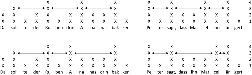
Following the structured preparation of the concept of prominence by Wagner et al. (Reference Wagner, Origlia and Avezani2015), the aspects that are particularly relevant for the definition of prominence will now be captured. For the sake of clarity, these aspects are listed:
Linguistic entity: As a linguistic entity that can be more or less prominent, here for the study of rhythm I am concerned with the syllable.
Stands out: Standout is defined in the context – it is lower for prominent syllables on the left and right than on the syllable itself. Furthermore, the perceptual evaluation of syllable prominence is used as a measure here.
Prosodic characteristics: Prosodic characteristics are defined in terms of lexical stress and accentuality. A distinction is made between stressable, non-stressable, stressed, and accented syllables (see Figure 22.1). Furthermore, rhythmic processes, for example in the form of the addition of prominence, are discussed for three consecutive unaccented syllables (see Figure 22.4).
Its environment: The environment refers to the linguistic material surrounding the syllable, specifically the surrounding syllables and words within a complement clause, as in (2).
Finally, we can consider the RhythmRule. Liberman and Prince (Reference Liberman and Prince1977) provide a systematization of the PRA (Sweet, Reference Sweet1876; Selkirk, Reference Selkirk1984). They show repair mechanisms or rhythmic processes that are activated when violations occur. These are summarized under the term RhythmRule (see Henrich, Reference Henrich2015). Assuming that the RhythmRule is active across domains (Henrich, Reference Henrich2015; Vogel et al., Reference Vogel, van de Vijver, Kotz, Kutscher, Wagner, Vogel and Vijver2015), it is worth recalling Example (2): On the one hand, the pronoun is not accented and, as a function word, is usually considered unstressed; however, it can gain prominence if we assume that the RhythmRule takes effect here. Thus, the sentence in (2) could be considered both rhythmic and nonrhythmic.
22.1.2 The Position of the German Pronoun in (Dis)rhythmic Sentences
In German, both subject-object (SO) and object-subject (OS) sequences are possible. Therefore, serialization is subject to various restrictions (Bader, Reference Bader2020). Uszkoreit (Reference Uszkoreit1986) formulated tendencies to produce the agent first – but also to prefix pronominal elements. For the object pronoun, which tends to fill the thematic role PATIENS, this implies variation in placement. Furthermore, the position has implications for the relative prominence of the pronoun, as, for example, Kügler (Reference Kügler2018) and Zerbian and Böttcher (Reference Zerbian, Böttcher, Calhoun, Escudero, Tabain and Warren2019) have shown for pronouns in the dative case.
Of interest for the study here is the position and prominence of the object pronoun, typically considered unaccented, in the midfield. In German, the midfield begins after the left clause bracket, which in verb-second clauses consists of the conjugated verb. In German complement clauses, the midfield begins after the complementizer. In the midfield, pronouns precede non-pronominal elements (Hoberg, Reference Hoberg1981).
Franz (Reference Franz2022) investigated the influence of rhythm on the position of the accusative object pronoun and the pronominal adverb. One of the questions was whether a manipulation of the stress structure of the neighboring words can influence the preferred placement of the pronoun in silent reading. In a questionnaire study, sentences were presented in pairs, each of which differed in terms of word position: Thus, the unaccented element of interest was either prefixed or in a position that could be considered canonical. Furthermore, sentence pairs differed in rhythmicity: Thus, in one of the two serializations, they were each more rhythmic, depending on the stress structure of the surrounding elements (see Figure 22.1).
The participants preferred the rear position of the unaccented elements in both structures studied. Furthermore, they preferred the prefixation of the elements more often when this led to rhythmic alternation. The results on the pronominal adverb are in line with those of Vogel et al. (Reference Vogel, van de Vijver, Kotz, Kutscher, Wagner, Vogel and Vijver2015).
Moreover, the findings illustrate that rhythmic well-formedness is not necessarily to be understood as a binary alternation of stressed and unstressed syllables. In the studied sentences with pronominal adverbs, rhythmic alternation indicates a dactylic structure, whereas in those with object pronouns, it is approximately trochaic (see Figure 22.1).
The sentences in Figure 22.1 illustrate the rhythmic structure of the sentences within the metrical grid. The sentence on the upper left shows a rhythmic, dactylic structure, and the one on the upper right shows a rhythmic, approximately trochaic structure. The lower part of the figure shows the variants that are unrhythmic due to a change in the word sequence. The spacing of the prominent syllables visualizes the rhythmicity in the structures as balanced (top) and unbalanced (bottom).
22.2 The Present Study
The current investigation is based on a study on the serialization of the German object pronoun in the accusative. The initial question of the study was whether a manipulation of the stress structure of the neighboring words can influence the placement of the German object pronoun in speech. This was done to shed light on the workings of rhythm in psycholinguistic models of speech production (for details, see Franz, Reference Franz2022). In this post hoc analysis, the respective materials and datasets are used in order to develop a measure of sentence rhythm.
In the respective picture-based study, participants produced complement sentences (as in 5) with the placement of the object pronoun (ihn, “him,” in bold) as the dependent variable (SO in 5a; OS in 5b).
(5a) Der Junge sagt, dass Markus ihn auslacht.
The boy says that Markus him laughs (at).
(5b) Der Junge sagt, dass ihn Markus auslacht.
The boy says that him Markus laughs (at).
“The boy says that Markus is laughing at him.”
The materials consisted of 32 sentences. Varying factors in the target sentences were the stress pattern of the embedded subject (iambic, trochaic) and of the embedded verb (initial stress, no initial stress). An overview of the rhythmic structure of the sentences is given in Figure 22.3. It was predicted that trochaic embedded subjects (see Figure 22.3, condition a and c) and verbs with no initial stress (see Figure 22.3, condition a and b) promote sentences with a fronted pronoun (OS). Additionally, animacy varied as a between-items factor with the matrix sentence subject being human or nonhuman.
Stimuli pictures were 64 black and white drawings developed with a professional illustrator. Each picture consisted of a left part symbolizing the matrix sentence (Der Junge sagt, “the boy says”) and a right part symbolizing the embedded sentence (dass Markus ihn auslacht, “that Markus is laughing at him”). The right parts of the pictures were mirrored (yielding 128 stimuli) to avoid word order effects due to spatial order (Figure 22.2). Finally, the variation in the degree of animacy was realized by exchanging Der Junge, “the boy,” with a nonhuman referent der Hase, “the rabbit.”
Visual stimuli.
Mirrored stimulus example for the target sentence Der Junge sagt, dass Markus ihn auslacht (SO)/Der Junge sagt, dass ihn Markus auslacht (OS), “The boy says that Markus is laughing at him.”
The results had shown that participants were more likely to produce OS when the embedded subject was of trochaic structure – however, this became significant only in the human subset (for a detailed analysis, see Franz, Reference Franz2022). The stress structure of the verb had no clear effect on sequencing. Furthermore, the analysis of perceptual syllable prominence had shown different processes of rhythmic accommodation. This is further differentiated in the current post hoc analysis.
22.2.1 Development of the Metric for Longer Structures Based on Shih et al. (Reference Shih, Grafmiller, Futrell, Bresnan, Vogel and Vijver2015)
For a clarification of the predictions, a closer look at the rhythmic structures of the target sentences is now taken due to the respective opposite predictions of verb and subject. Figure 22.3 shows the number of rhythmic violations according to Shih et al. (Reference Shih, Grafmiller, Futrell, Bresnan, Vogel and Vijver2015) before and after the embedded subject in all four conditions and for both variants (SO/OS). The problem with this “local” definition of rhythm will be discussed in the following.
Development of the balance measure.
Example sentences in conditions (a–d) and the two serialization options (SO and OS). The bold portions indicate the syllables with lexical accent. The numbers below the text represent the number of rhythmic violations (stress clash/stress lapse) according to Shih et al. (Reference Shih, Grafmiller, Futrell, Bresnan, Vogel and Vijver2015). The digits to the right of each sentence show the sum of rhythmic violations. The arrow in condition (d) shows the change that was made here to represent the quality of lapse and clash (this value is used for the balance measure). The balance measure results from a subtraction of the two values of a sentence; the ranking index (R) shows the respective strength for a preference of OS or SO (see the text for details).
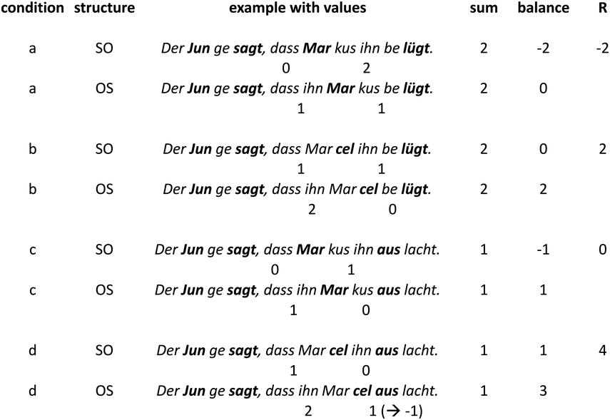
Shih et al. (Reference Shih, Grafmiller, Futrell, Bresnan, Vogel and Vijver2015) restrict their analysis to genitive constructions that contain at most two accents – a single or local determination of *LAPSE and *CLASH is thus sufficient. But what happens when the rhythmic structure of an entire sentence is to be determined? With about three accents, two measures could be summed up, and the one containing fewer violations in the sum would be more rhythmic. To test this, let’s take a closer look at the target sentences of the experiment. Figure 22.3 shows the summed violations to the right of each sentence. It turns out that summation does not make clear predictions. With the exception of condition (d), the two variants are predicted to be equivalent in all conditions. In contrast, there is an apparent varying distance between the respective accented syllables, as, for example, in the comparison of OS and SO in condition (a) – so far, however, there is no measure that can capture this balance. A first attempt consists in subtracting the two values calculated according to Shih et al. (Reference Shih, Grafmiller, Futrell, Bresnan, Vogel and Vijver2015) in the sentence. For this purpose, the conditions are examined in more detail.
22.2.1.1 Condition (a)
Based on the local rhythmic predictions, it has already been established above that in condition (a) the prefixation of the pronoun is predicted because of the iambic verb and trochaic subject. Looking at the sentence as a whole, however, this prediction seems less clear (Figure 22.3): The prefixation of ihn, “him,” generates a *LAPSE with the unstressed complementizer dass, “that” (*dass ihn, formalized in 6a); at the same time, the encounter of the unstressed final syllable of the trochaic subject and the unstressed initial syllable of the iambic verb generates another *LAPSE (*-kus be-, formalized in 6b).
(6a) |2-1| = 1
(6b) |2-1| =1
In the SO structure less predicted on the basis of local rhythmicity, a double *LAPSE arises to the right of the subject by the unstressed final syllable of the trochaic name, the unstressed pronoun, and the initial syllable of the iambic verb (-**kus ihn be-, formalized in 7b). To the left of the subject, no violation occurs with an alternation of stressed matrix verb, unstressed complementizer, and stressed initial syllable of the embedded subject (sagt, dass Mar-, formalized in 7a).
(7a) |1-1| = 0
(7b) |3-1| = 2
Intuitively, it seems clear that a “balanced” distribution of violations should be preferred here, and thus an OS structure. Also, it has already been shown that both trochaic and dactylic rhythms can influence word order preferences, and thus a pure alternation of stressed and unstressed syllables is not mandatory for rhythmic well-formedness. However, the sentences in this study have neither a pure trochee nor a pure dactyl, and formal addition generates the same number of violations (exactly two each) in condition (a) for OS and SO.
If we now assume that the spacing of the accents should be balanced, one value can be subtracted from the other for a balance measure, and an optimal balance measure is at a value of 0 (formalized in 8a). In this way, the formula of Shih et al. (Reference Shih, Grafmiller, Futrell, Bresnan, Vogel and Vijver2015) can be extended for longer structures. When applied to condition (a), a 0 (formalized in 8b) is obtained for the OS structure, and a 2 (formalized in 8c) for the SO structure. In this example, therefore, the OS variant formalized in (8b) is predicted with a balance measure of 0.
(8a) | value left – value right |
(8b) | 1-1 | = 0
(8c) | 0-2 | = 2
22.2.1.2 Condition (b)
Based on the local rhythmic predictions, it has already been established above that in condition (b), because of the iambic verb, the prefixation of the pronoun is predicted (OS; see Figure 22.3). At the same time, the iambic subject favors an SO structure, leaving the prediction unclear without the total sentence. The two variants in condition (b) each have two violations: In the SO structure, they are evenly distributed, respectively, with the two unstressed syllables of the complementizer and the first syllable of the iambic subject (*dass Mar-), and the pronoun together with the first syllable of the iambic verb (*ihn be-). In the OS structure, on the other hand, the violations of *LAPSE gather with the complementizer, the pronoun, and the first syllable of the iambic subject in a double *LAPSE structure (**dass ihn Mar-). Transferred to the formula in (9a), this implies an ideal balance measure for the SO structure in (9b), but not for the OS structure in (9c). SO is therefore predicted for condition (b).
(9a) | value left – value right |
(9b) | 1-1 | = 0
(9c) | 0-2 | = 2
22.2.1.3 Condition (c)
The local rhythmic predictions favor an OS structure due to the trochaic subject and an SO structure due to the trochaic verb. As in condition (b), the prediction due to local rhythmicity is unclear for condition (c). Unlike in condition (b), it remains so when looking at the complete sentence: The pronoun produces a *LAPSE with one of the adjacent syllables in both positions (SO and OS), with the second syllable of the trochaic subject (*-kus ihn) in the OS variant, and with the complementizer (*dass ihn) in the SO variant (see Figure 22.3). This is illustrated by the formulas in (10b) and (10c). For condition (c), therefore, there is no clear prediction by the rhythmic structure.
(10a) | value left – value right |
(10b) | 0-1 | = 1
(10c) | 1-0 | = 1
22.2.1.4 Condition (d)
In the OS example of condition (d), we obtain two violations of *LAPSE before the embedded subject (Marcel), resulting from the unstressed complementizer, the pronoun, and the initial syllable of the iambic subject (**dass ihn Mar-; see Figure 22.3). (11a) formalizes the *LAPSE structure according to Shih et al. (Reference Shih, Grafmiller, Futrell, Bresnan, Vogel and Vijver2015) (|number of unstressed syllables - 1|). Furthermore, the coincidence of the stressed second syllable of the iambic subject and the initial syllable of the trochaic verb (*-cel aus-), which is also stressed, creates a *CLASH (marked by 1), which is formalized in (11b) according to Shih et al. (Reference Shih, Grafmiller, Futrell, Bresnan, Vogel and Vijver2015).
(11a) |3-1| = 2
(11b) |0-1| = 1
In the SO example of condition (d), the (local) rhythmic structures look more balanced: No rhythmic violation occurs to the right of the embedded subject because the unstressed pronoun stands alone between the stressed final syllable of the subject and the stressed initial syllable of the verb (-cel ihn aus-). (12a) formalizes the alternating structure. To the left of the embedded subject, the unstressed complementizer and the unstressed initial syllable of the iambic subject create a *LAPSE (dass Mar-); this is formalized in (12b).
(12a) |1-1| = 0
(12b) |2-1| = 1
Thus, in condition (d), an SO structure is more rhythmic than an OS structure. The strength of this preference will be discussed in the following.
22.2.1.5 Reflections on the Quality of Lapse and Clash
Transferring the values of condition (d) to the balance measure introduced above yields a counterintuitive result: Although the OS structure has significantly less balanced spacing of accents compared to the SO variant, the balance measure (13a) yields the same result for both variants (OS in 13b, SO in 16c).
(13a) | value left – value right |
(13b) | 2-1 | = 1
(13c) | 0-1 | = 1
This is explained by the fact that Shih et al. (Reference Shih, Grafmiller, Futrell, Bresnan, Vogel and Vijver2015) are only concerned with local rhythmicity, not with the balance of larger sections, and the sentences considered here so far have only had lapses as violations. Apparently, however, *LAPSE and *CLASH have different effects on the spacing of accents in a sentence. While lapses move them gradually apart, a clash has the opposite effect: The stressed syllables of the accented words meet directly, preventing rhythmic alternation.
To account for this difference, the modulus proposed in Shih et al. (Reference Shih, Grafmiller, Futrell, Bresnan, Vogel and Vijver2015) is omitted. In this way, the values at a *LAPSE and a *CLASH receive different signs, producing values that relate not only to the number of rhythmic violations but also to their quality (see Figure 22.3). (14a) illustrates the corresponding rhythmic measure. (14b) shows the resulting balance measure, and (14c) and (14d) formalize the balance measures for the SO variant (14c) and the OS variant (14d) in condition (d).
(14a) (Number of unstressed syllables between two stressed syllables -1)
(14b) (value left) – (value right)
(14c) (1-1) – (2-1) = -1
(14d) (2-1) – (0-1) = 2
It turns out that (14c) and thus the SO variant is closer to 0 than the OS variant (14d). Consequently, the new rhythm and balance measure predicts the rhythmicity of the two word order variants according to the visual impression: SO is more rhythmic than OS in condition (d). Figure 22.3 summarizes the discussed values per condition for OS and SO, respectively. The optimal rhythmic structure is indicated by a balance measure (= 0). It can be seen, as in the analysis of local rhythmicity, that in condition (a) OS is predicted, in condition (c) there is again no clear prediction, and conditions (b) and (d) each prefer SO. The extent to which the development of the balance measure goes further than the previous analysis will be shown below.
22.2.1.6 Development of a Rhythmical Ranking
In the previous section, a measure was developed that maps the rhythmic structure within three accented syllables, taking into account not only the number of rhythmic violations but also their quality. This was done by qualitatively distinguishing *LAPSE and *CLASH and integrating them into the measure. In this way, for each possible utterance within one of the experimental conditions, there now exists a balance measure that expresses the rhythmic well-formedness of the sentence: The farther the value is from 0, the more unrhythmic the sentence is. Thus, the structure with a value closer to 0 is predicted. According to this measure, it can be stated that in condition (a) OS is predicted, in condition (c) there is no clear prediction, and conditions (b) and (d) both predict SO.
The gain of the balance measures now is that they are meaningful not only within conditions but also between conditions. If we first relate the balance measures within each condition to each other by adding them up, we obtain a value that is called ranking index (R) (see Figure 22.3). This value represents the strength of the predictions – the larger its distance from 0, the stronger is the prediction.
Accordingly, the prediction for SO is strongest in condition (d) with an R of 4, followed by condition (b) with an R of 2. Not further specified is the probability for SO in condition (c) with an R of 0, and it is finally least likely in condition (a) with an R of -2. The strength of the predictions for SO is consequently distributed between the conditions, as in (15a). Accordingly, the predictions for OS per condition are exactly opposite: OS is most likely in condition (a), followed by conditions (c), (b), and (d). This is summarized in (15b).
(15a) prediction SO: d >> b >> c >> a
(15b) prediction OS: a >> c >> b >> d
Accordingly, the balance measures allow us to map a graded predictive power and also show that the experimental design allows for rhythmically well-formed SO sentences rather than correspondingly rhythmic OS sentences. This might explain the rather weak rhythmic effects on sequence preferences (see Franz, Reference Franz2022, for details).
Moreover, the gradations separated into OS and SO in (15a) and (15b) can be summarized into a single four-level ranking. Thus, OS sentences of condition (a) and SO sentences of condition (d) are the most likely – these form level 1 in the ranking. Accordingly, OS sentences of condition (d) and SO sentences of condition (a) are the least likely – these form level 4 in the ranking. The prediction is simply that level 1 sentences should be the most frequent, followed by levels 2, 3, and 4. The complete four-level ranking is summarized in (16a–d). In each case, the conditions are in parentheses after the preferred structure. The corresponding example sentences are shown in Figure 22.3.
(16a) Level 1: SO(d), OS(a)
(16b) Level 2: SO(b), OS(c)
(16c) Level 3: SO(c), OS(b)
(16d) Level 4: SO(a), OS(d)
22.2.2 Methods
22.2.2.1 Participants
Fifty-one experimental participants (age: 19–81 years; M = 41.8; SD = 18) with German as (one of) their first language(s) took part in the study. Thirty-one of them were female. Three of the participants reported being bilingual (German/Polish, German/Vietnamese, and German/French). The participants were recruited through the subject pool of the Max Planck Institute for Empirical Aesthetics in Frankfurt, Germany. All reported normal or corrected-to-normal vision and no severe hearing, vision, speech, or neurological impairments. All participants gave their written consent for voice recordings to be made and for their data to be processed pseudonymously. Each participant received an expense allowance of 15 euros. All participants had the opportunity to discontinue the experiment at any time without giving reasons.
22.2.2.2 Materials
Materials used are given in Sections 22.2 and 22.2.1.
22.2.2.3 Procedure
The 128 stimuli were distributed over four different lists. Each list contained 32 stimuli, balanced by item and condition. Each of the lists was subjected to the same pseudorandomization using MIX (Casteren and Davis, 2006).
In addition, 32 stimuli were added to each sequence that contained the target sentences in written form so that they could be read aloud by participants. In a final step, pictorial and written stimuli were mixed in such a way that four blocks of 16 stimuli each were arranged consecutively. The first block consisted of written sentences, the second of the corresponding pictorial stimuli, the third of written stimuli, and the fourth again of the corresponding pictorial stimuli. (17) shows a schematic representation of a sequence.
(17) read out 16 sentences >> name 16 pictures >> read out 16 sentences >> name 16 pictures
The complete experiment took place in the laboratory of the Max Planck Institute for Empirical Aesthetics, in a soundproof room where the participant sat alone at a desk in front of a computer screen. The experimenter (the author of this chapter) controlled the experiment from an adjoining room, and contact with the participant was via an intercom system. The experiment was preceded by a distinct familiarization phase with the target items and target structures (for details, see Franz, Reference Franz2022).
The presentation of the sequences explained above and the recording of the individual utterances were performed in Matlab. Accordingly, 64 WAV files were created per participant – in the context of this chapter, only those that were created in response to the pictorial stimuli will be discussed (32 recordings per participant). The further parts of Experiment 1 (runs 2–4) were performed according to the variable speed of each participant only with those who had at least 10 minutes of their 60-minute session left. These further parts corresponded to the test phase of Experiment 1. Experiment 2 (a writing task) will not be discussed here.
22.2.2.4 Analysis
All participants’ utterances were subsequently transcribed and coded by three independent student assistants. First, all valid utterances were coded as to whether the pronoun in the complement clause was produced before (1: dass ihn Marcel massiert, “that Marcel massages him”) or after the embedded subject (0: dass Marcel ihn massiert, “that Marcel massages him”). An utterance was considered valid if it contained one of the two required matrix sentences (der Hase träumt, “the rabbit dreams”/Der Junge sagt, “the boy says”) as well as a complement sentence in the present active tense with bisyllabic verb, bisyllabic subject, and the object pronoun ihn, “him.” The factors of stress structure of embedded verbs and subjects (2: iambic/1: trochaic) were made on the basis of the utterance actually produced.
Additionally, the degree of animacy of the matrix subject was annotated (1: human/0: nonhuman), as well as the spatial arrangement (left/right) of the figures representing the subject and object of the complement clause in the stimulus (referent of object on the left: 1; referent of object on the right: 0; see Figure 22.2).
Further, the fluency of the utterances was coded on a three-point scale (1: The utterance contained no pauses, filler words, self-corrections, repetitions, or the like; 0.5: The utterance was interrupted only before the complement clause by one or more of the above-mentioned fluencies; 0: The utterance was [also] interrupted in the complement clause by one or more of the above-mentioned fluencies). Only the utterances with fluent complement clauses (fluency at least 0.5) were integrated into the analysis (n = 1819) in order to allow for an audible comparison between the prominence of the pronoun and that of the adjacent syllables during annotation.
Finally, the syllable prominence of the pronoun was coded. A student assistant with German as one of their first languages annotated the utterances. A distinction was made here between unstressed (n = 1355), stressed (n = 196), and reduced (n = 268) syllables, following Vogel et al. (Reference Vogel, van de Vijver, Kotz, Kutscher, Wagner, Vogel and Vijver2015).
22.2.3 Results
22.2.3.1 Proportions of Sentences
Table 22.1 shows the proportions of utterances produced according to the rhythmic ranking presented. The whole dataset shows a tendency according to the prediction (stage 1 is the most frequent, stage 4 the least frequent), with an irregularity in stages 2 and 3 (the latter proportion is larger).
| Ranking and word order | ||||
|---|---|---|---|---|
| Ranking index | ||||
| Dataset fluent sentences | 1 | 2 | 3 | 4 |
| OS and SO n = 1819 | 26.8 | 24.6 | 25.2 | 23.4 |
| subset OS n = 546 | 23.8 | 28 | 24 | 24.2 |
| subset SO n = 1273 | 28.7 | 23.1 | 25.5 | 22.7 |
| subset human n = 969 | 27 | 25,9 | 24,3 | 22,8 |
In addition, two subsets were formed, and these are also shown in Table 22.1 in terms of the rhythmic ranking. In the subset with SO structures, a similar picture appears as in the entire dataset, but here even more pronounced in its expression. In the subset with OS structures, on the other hand, no comprehensible pattern is discernible. It is noticeable here that level 2 is represented relatively frequently; this is taken up again below.
In summary, the descriptive analysis of the utterances reveals frequencies that tend to match the predictions of the ranking. Thus, sentences assigned to level 1 occurred most frequently, while those assigned to level 4 occurred least frequently. It is also notable that level 3 sentences were chosen more frequently than those assigned to level 2. However, this pattern only applies to the more frequent SO sentences; no such systematic pattern is apparent for the OS sentences. Moreover, variation in animacy seems to affect the results: The subset that does not vary with respect to animacy (the human subset) adheres to the predictions (also in relation to levels 2 and 3), albeit very slightly.
For statistical analysis, a generalized linear mixed-effects regression model (GLMER; Bates et al., Reference Bates, Mächler, Bolker and Walker2015) was computed in R statistical software (version 4.0.2; R Core Team, 2020). The selected model computed successive distances (frequencies) between levels of the rhythmic ranking (taking into account sentence structures OS and SO). Covariates included were, in addition to fluency of utterance, spatial arrangement (mirror) and animacy of the antecedent of the pronoun. Both item and participant were integrated as random effects. In addition, participant and run were coupled as embedded factors (Common Extensions | Mixed Models with R [m-clark.github.io]). Participant and run were thus considered embedded, as there were potentially four runs for each participant.
The covariates did not assume a significant magnitude, except for the spatial ordering. Regarding the ranking, the model for the whole set (OS and SO) shows a highly significant distance between levels 1 and 2 in the predicted direction. The negative sign (z = -1.7) between levels 2 and 3 illustrates the tendency against the prediction (there were more level 3 sentences than level 2 sentences), this difference taking on a marginally significant size (see Table 22.2).
| Model (GLMER) ranking | ||||
|---|---|---|---|---|
| Estimate | Std. Error | z value | Pr(>|z|) | |
| (Intercept) | −0.79269 | 0.14425 | −5.495 | <0.0001 *** |
| Ranking 2-1 | 0.49570 | 0.15097 | 3.283 | 0.00103 ** |
| Ranking 3-2 | −0.26226 | 0.15114 | −1.735 | 0.08271 † |
| Ranking 4-3 | 0.18580 | 0.15308 | 1.214 | 0.22484 |
| Mirror | 0.11064 | 0.05353 | 2.067 | 0.03875 * |
| Animacy | −0.06936 | 0.05361 | −1.294 | 0.19573 |
| Fluent 1 | −0.18068 | 0.14335 | −1.260 | 0.20754 |
Signif. codes: 0 “***” 0.001 “**” 0.01 “*” 0.05 “.” 0.1 “†”
22.2.3.2 Syllable Prominence
Based on the previous analysis, a conflation of syllable prominence and ranking will now be performed. It is predicted that the prominence level of the pronoun will vary systematically with the rhythmic ranking. In particular, the pronoun should be classified as stressed more often in the sense of accommodation in stage 4, which is classified as unrhythmic, than in the more rhythmic stages 1, 2, and 3.
To illustrate, the prominence levels defined at the beginning of this chapter are presented here. Syllable prominence was defined as a four-level quantity consisting of accented syllables, stressed syllables, stressable syllables, and unstressable syllables. Figure 22.4 shows a sentence in the context of this model. Here, the pronoun as a function word is initially considered unstressed. The predicted gain or reduction of prominence is marked by parentheses around the corresponding cross (lower panel) or its deletion (upper panel).
Varying prominence on the pronoun.
Upper panel: Prominence reduction on the pronoun. Lower panel: Addition of prominence on the pronoun.
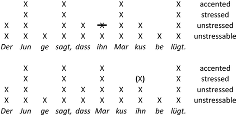
Figure 22.4 Long description
The words are der Junge sagt, dass Markus ihn belügt. Each word has a series of "X" marks in a grid. The columns of "X" marks correspond to different accentuation categories: accented, stressed, unstressed, and unstressable.
For the analysis, all (semi-)fluent sentences were analyzed in terms of rhythmic ranking (1–4) and annotated syllable prominence (reduced, unstressed, stressed). Table 22.3 shows the merging of the categories in absolute numbers (n = 1819). The pronouns rated as unstressed are proportionally represented with similar frequency in the levels – with the exception of levels 2 and 3. Thus, the pronoun in level 3 was rated as unstressed with striking frequency, followed by levels 1, 4, and 2. For the other two degrees of prominence, a clear pattern emerges: According to the prediction, the proportion of stressed pronouns successively increases with decreasing rhythmicity. In the opposite direction, the proportion of reduced pronouns successively decreases with decreasing rhythmicity. Figure 22.5 visualizes the results.
| Ranking and prominence degree | ||||
|---|---|---|---|---|
| Ranking index | ||||
| Prominence degree | 1 | 2 | 3 | 4 |
| Reduced | 103 | 90 | 50 | 25 |
| Unstressed | 350 | 312 | 359 | 336 |
| Stressed | 35 | 44 | 51 | 64 |
Rhythmic ranking and degrees of prominence.
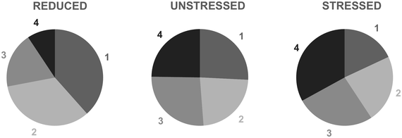
Figure 22.5 Long description
The category wise major to minor sectors representing the levels of rhythmic ranking are as follows. Reduced. 1, 2, 3, and 4. Stressed. 4, 3, 2, and 1. Unstressed. 3, 4, 1, and 2.
It should be particularly emphasized at this point that these systematics are also evident in levels 2 and 3, because the frequency distribution of these two levels had occurred in reverse order in the analysis of the previous chapter, contrary to prediction.
In addition, pronouns referring to a nonhuman referent (n = 850) were rated as stressed (n = 100) more often than those referring to a human referent (n = 969; n = 94 rated as stressed), with the latter being rated as reduced (n = 159) more often than the former (n = 109).
Finally, the relationship between annotated syllable prominence and ranking was statistically tested. For the analysis, a GLMER model (Bates et al., Reference Bates, Mächler, Bolker and Walker2015) was computed in R statistical software (version 4.0.2; R Core Team, 2020). The chosen model computes successive distances (frequencies) between levels of rhythmic ranking, here in the context of annotated syllable prominence. To do justice to the binomial character of the model, it refers to a rescaled prominence. This means that the previously three-level prominence in the model distinguishes only between those pronouns that were scored as reduced and all others. Consequently, in this model, the reduced syllables (coded as -1) were set apart from all others (coded as 0).
Included covariates were, in addition to fluency of utterance, spatial arrangement (mirror) and animacy of the antecedent of the pronoun. Both item and participant were integrated as random effects. In addition, participant and run were coupled as embedded factors, as in the previous section.
Table 22.4 summarizes the results of the model. It revealed a significant difference between ranking levels 3 and 4, and a highly significant difference between levels 2 and 3. Furthermore, animacy significantly affected the perceived syllable prominence of the pronoun.
| Model (GLMER) ranking | ||||
|---|---|---|---|---|
| Estimate | Std. Error | z value | Pr(>|z|) | |
| (Intercept) | 2.11668 | 0.18864 | 11.221 | <0.0001 *** |
| Ranking 2-1 | 0.03067 | 0.17347 | 0.177 | 0.859650 |
| Ranking 3-2 | 0.74253 | 0.20053 | 3.703 | 0.000213 *** |
| Ranking 4-3 | 0.65330 | 0.26054 | 2.508 | 0.012158 * |
| Mirror | −0.02387 | 0.07188 | −0.332 | 0.739850 |
| Animacy | −0.14641 | 0.07183 | −2.038 | 0.041521 * |
| Mirror:Animacy | 0.09343 | 0.07178 | 1.302 | 0.193072 |
Signif. codes: 0 “***” 0.001 “**” 0.01 “*” 0.05 “.” 0.1 “†”
22.3 Discussion
In the present chapter, a new metric for the evaluation of the rhythmic well-formedness of sentences was developed. This measure is based on the assumption that not only is the local rhythm relevant for the rhythmicity of a structure (stress lapse or stress clash at a defined position) but also the rhythm of the entire structure. Following the results on the relevance of trochaic and dactylic rhythm (Franz, Reference Franz2022), and the work of Hanna (Reference Hanna2003) and Vogel et al. (Reference Vogel, van de Vijver, Kotz, Kutscher, Wagner, Vogel and Vijver2015), the hypothesis was developed that the balanced spacing of accented syllables is the relevant measure. Under this assumption, the measure of Shih et al. (Reference Shih, Grafmiller, Futrell, Bresnan, Vogel and Vijver2015) of local rhythm was used and further extended. The result covers structures with up to three accented syllables and is shown schematically in (18). An ideal sentence rhythm lies at the value zero in (18b). Deviations are equally weighted in the positive and negative range.
(18a) Local rhythm: (n unstressed syllables between two stressed syllables -1)
(18b) Balance measure: (value left) - (value right)
The metric was developed during a post hoc analysis of a picture-based production study in Franz (Reference Franz2022). One of the questions of this study was whether a manipulation of the stress structure of the neighboring words (iambic or trochaic) can influence the preferred placement of the German object pronoun (SO/OS). The rhythmic quality of the target sentences of the respective study was then re-evaluated as predicted by the new metric, resulting in a rhythmic ranking consisting of four levels (descending in rhythmicity).
In order to strengthen the new metric empirically, the chapter presented two analyses. The first analysis evaluated how the structures produced by the participants were distributed on the rhythmic ranking. According to the prediction, level 1 sentences should occur more frequently than those of levels 2, 3, and 4. The results partially confirmed this prediction: Overall, the frequencies were distributed according to the ranking with an inverted order of levels 2 and 3. However, only the difference between levels 1 and 2 was significant. The evaluation showed that the ranking applies primarily to the SO sentences, not to the OS sentences. Consequently, the results indicate that the participants construct the sentences in such a way that the preferred SO structure can be realized as rhythmically as possible. Accordingly, the frequencies of SO sentences tended to follow the rhythmic ranking, but the frequencies and proportions of OS sentences were unsystematic (with respect to the ranking).
Finally, the numbers in the human subset were found to be consistent with the predictions. Although the influence of animacy did not reach significance in the statistical model, the descriptive results do suggest that it is a confounding factor here. Respectively, in the study in Franz (Reference Franz2022), rhythmic influences on pronoun placement were found to reach the significance level only when animacy did not vary (see also McDonald et al., Reference McDonald, Bock and Kelly1993; Franz et al., Reference Franz, Kentner and Domahs2021). Therefore, in a future application and further development of the metric, care should be taken to avoid animacy differences. This was also relevant for the analysis of syllable prominence.
In the second analysis, the rhythmic ranking was reviewed in terms of perceived prominence of the pronoun. The results strengthened the predictions of the measure in the sense that syllable prominence varied systematically with predicted rhythmicity. Thus, pronouns were perceived as stressed especially in sentences classified as unrhythmic, and as reduced in rhythmic sentences. Only the latter result could be statistically tested and reached the significance level. Furthermore, animacy affected perceived syllable prominence; that is, pronouns referring to human referents were perceived as less prominent than those referring to nonhuman referents. However, the results should be interpreted cautiously, since the second analysis was based on perceived prominence by one person only (for problems with this kind of evidence, see Bruggeman et al., Reference Bruggeman, Schade, Włodarczak and Wagner2022). Further, the statistical model could only be done with the reduced pronouns (the systematics were shown with the stressed pronouns in the descriptive analysis).
Nevertheless, the results concerning the proportions of the produced structures in combination with the results on syllable prominence allow for a first empirical support of the new metric. In the context of the aim of this study, the introduced metric made it possible to systematize the rhythmicity visible in the metrical grid of the studied sentences. In its existing form, the metric works for structures with three accented (or otherwise prominent) syllables and, as such, is also applicable to structures not studied in this chapter.
Besides a phonetic validation, a next step would be to apply the metric to further structures. In doing so, a promising continuation of the project would be to consider aspects of prosodic boundaries. Thus, it should be investigated whether and to what extent the occurrence of prosodic boundaries between the prominent syllables affects sentence rhythmicity. One of the many possibilities is to change the meter (the spacing of prominent syllables) within an utterance (Vogel et al., Reference Vogel, van de Vijver, Kotz, Kutscher, Wagner, Vogel and Vijver2015). In the work presented here, a new metric was developed as an extension to Shih et al. (Reference Shih, Grafmiller, Futrell, Bresnan, Vogel and Vijver2015), providing a further basis for the study of sentence rhythm.
Summary
The present chapter presents a metric for the formal computation of the rhythmic soundness of a sentence. The measure is developed in a post hoc analysis of a speech production experiment on the influence of rhythm on the placement and prominence of the German object pronoun ihn [English “him”].
Implications
Future studies in the field of sentence rhythm can use the metric to formally capture rhythmic coherence when it goes beyond a binary alternation of stressed and unstressed syllables. The developed formal distinctions of stress lapse and stress clash and their relationship within a sentence could be evolved to make them useful for longer structures.
Gains
The present elaboration demonstrates that rhythmic soundness is not necessarily equivalent to a binary alternation of stressed and unstressed syllables. This should be kept in mind when developing linguistic stimuli. Rhythmicity rather depends on the composition of stress lapses and clashes – which can be formally grasped using the metric.
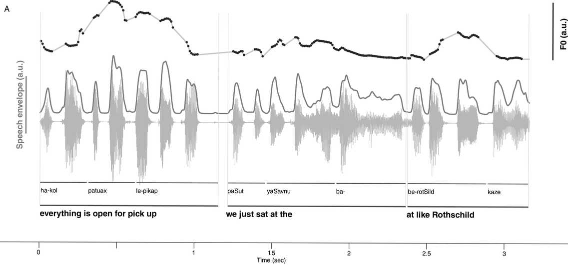

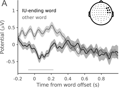
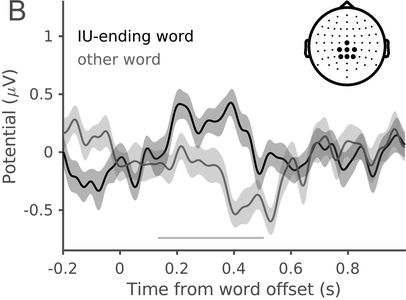
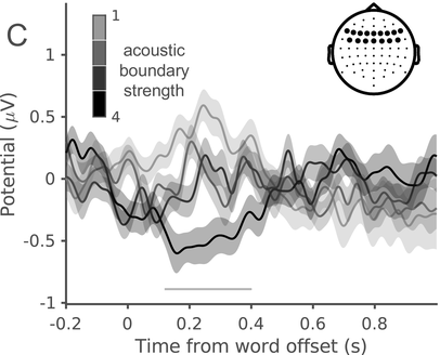
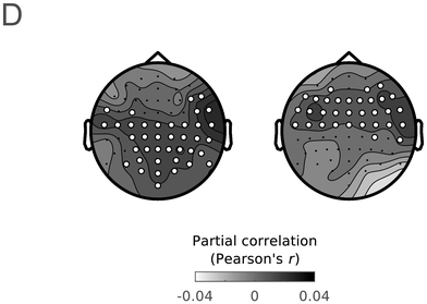
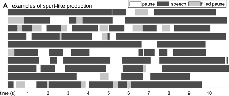
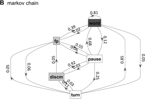
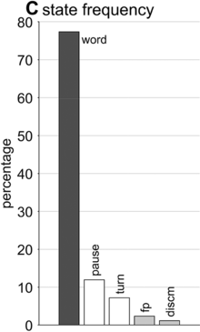
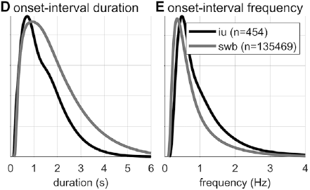
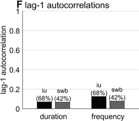
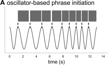
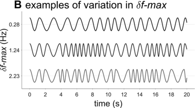
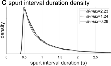
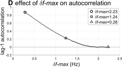
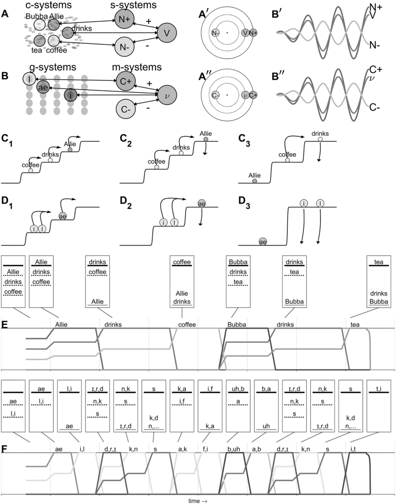
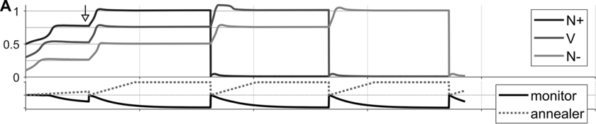
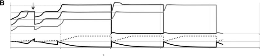
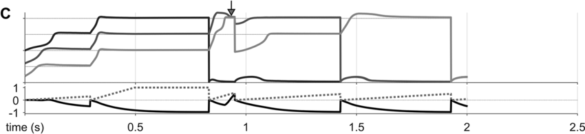
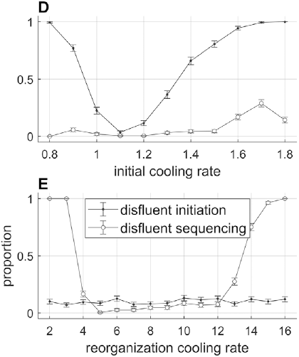
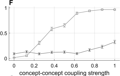
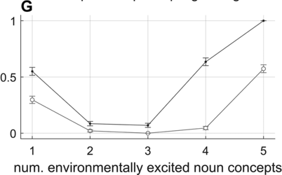
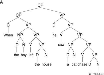
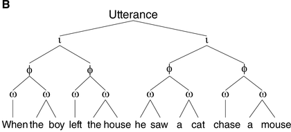
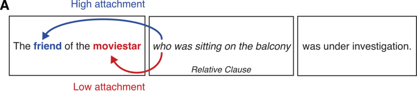
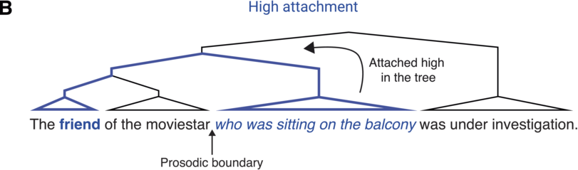
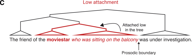
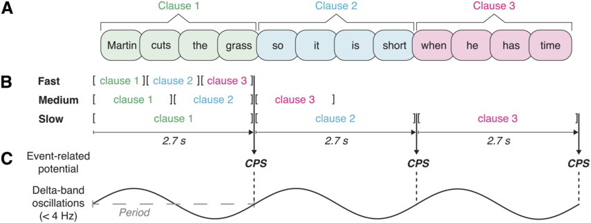
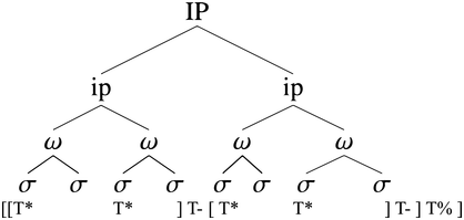
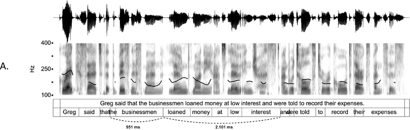
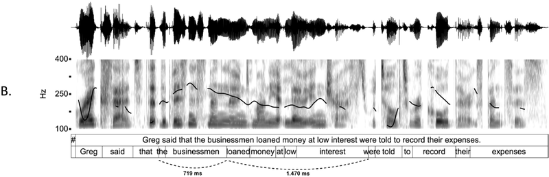
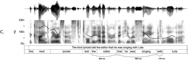
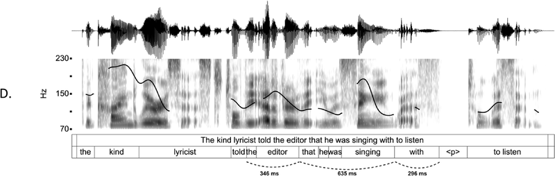
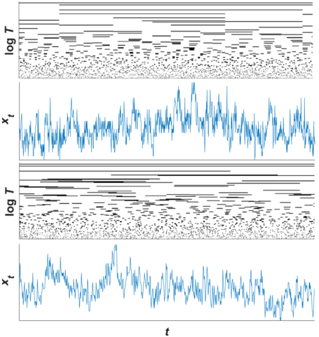
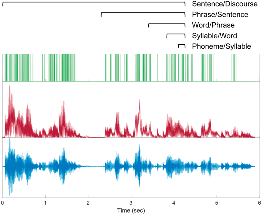
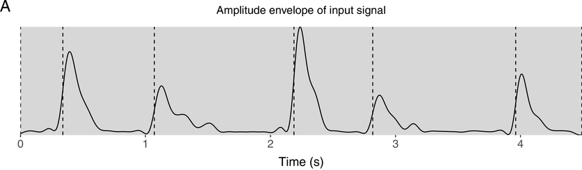
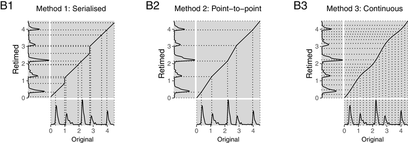
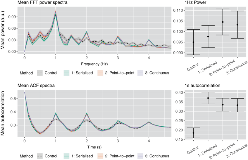
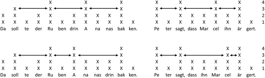

 Open access