1. Introduction

Many curious white spots of 1–10 cm diameter were found on wet snow (~10 mm thick) on the morning of 1 November 2009 in Kitami and Oketo in Hokkaido, Japan. We refer to this phenomenon as ‘white spotted wet snow’. Most of the white spotted wet snow was observed on an asphalt paved road, but it was also observed on concrete and tile pavements, which are almost impermeable to water.

This phenomenon has been noted in Japan previously. Reference NohguchiNohguchi (1984) wrote that ‘After snow deposition of 1 or 2 cm in thickness and rain, snow with air bubbles will appear’ (translated from Japanese). He presented a photograph of white spotted wet snow, as did Reference HayashiHayashi (1985). Reference Kominami and YokoyamaKominami and Yokoyama (2004) reported observations of ‘white spotted wet snow’ at Jyoetsu, Niigata Prefecture, on 7 March 2004. The Daily News in Niigata (local community newspaper published in Niigata district in Japan) published a beautiful picture of white spotted wet snow on 28 February 2004, which was taken by Noriko Kawano on 25 February 2004 at Joetsu, Niigata. All these reports describe observations of white spotted wet snow. However, there have been no investigations of the formation process, meteorological conditions that lead to its formation, its vertical structure and the horizontal pattern of the white spots. One of the authors (S.T.) has lived in Kitami for more than 30 years but had not seen this phenomenon previously.

This paper presents the characteristics of white spotted wet snow observed in Kitami and Oketo on 1 November 2009.

2. Characteristics Of White Spotted Wet Snow

Figure 1 shows the study area of Kitami, Oketo, Bihoro and Rubeshibe in eastern Hokkaido, Japan. Joetsu in Niigata Prefecture is also shown. Figure 2 shows photographs of white spotted wet snow on an asphalt pavement in front of the house of one of the authors (T.K.) in Kitami on 1 November 2009. Figure 2a shows the widespread distribution of white spotted wet snow on the road. The snow was 5–10 mm thick at the time of the photograph. Figure 2b shows the horizontal distribution of white spotted wet snow, in which air bubbles of ~40 mm diameter are regularly distributed. A close-up photograph of a white spot is shown in Figure 2c. Transparent ice grains can be clearly seen floating on water. When one of the authors was observing the white spotted wet snow, small ice pellets 1 mm in diameter were also falling. These ice pellets deposited on the mixed ice–water layer (Fig. 2c).

Fig. 1.

Location of observations (Kitami, Oketo, Bihoro and Rubeshibe) in Hokkaido, Japan. Joetsu in Niigata Prefecture is also shown.

Fig. 2.

White spotted wet snow in Kitami (1 November 2009). (a) White spotted wet snow on a road (taken at 09:01). (b) Horizontal distribution of white spotted wet snow (09:00) and (c) close-up photograph (09:35). (d) Air released from the white spots (09:36). (e) After the disappearance of the white spots (11:32) at the same location shown in (a–d).

The centres of the white spots were raised ~1 mm above the snow. When the spots were pushed, they moved easily. When the ice pellets were removed from the surface of the mixed ice–water layer near the spots, air was released from them (Fig. 2d). These simple experiments revealed that the white spots were formed by air bubbles below the mixed ice– water layer. Figure 2e shows the condition 3 hours after the photograph in Figure 2d was taken. Some ice grains have clustered at intervals of several centimetres. Because the heat conductivity of air at 0°C (0.024 W m^–2 K^–1) is ~1/20 of the heat conductivity of water at 0°C (0.561 W m^–2 K^–1), the ice grains on the white spots did not melt, whereas ice grains located elsewhere did.

The vertical structure of the spots was examined and is shown in Figure 3a. A thin water layer (2–5 mm thick) was present on the asphalt pavement, and a mixed ice–water layer (2–3 mm thick) was present on the thin water layer. Ice pellets 1 mm in diameter were enclosed in the mixed ice– water layer. There was an air bubble between the two layers. We consider that the thickness of the bubbles was close to the surface height difference of 1 mm. We measured the thickness of air bubbles in the white spotted wet snow by measuring the air volume and diameter of white spots in the winter of 2010/11. Based on 79 measurements, the average thickness was 1.1±0.5 mm. This value is close to the observed surface height difference in Kitami on 1 November 2009. Because the reflectance of ice for the sodium D line (1.3090 for ice at –3°C; Reference HobbsHobbs, 1974) is similar to that of the water for the sodium D line (1.3339493 for water at 0°C: Reference Eisenberg and KauzmannEisenberg and Kauzmann, 1969), it was difficult to identify ice grains in water. Consequently, the areas around the white spots appeared to be dark, like the underlying asphalt.

Fig. 3.

(a) Vertical section of white spotted wet snow. (b) Reflection and refraction of sunlight in the white spotted wet snow.

Figure 3b shows the scattering process of sunlight in white spotted wet snow. Because the reflectance of air at 0°C is 1.000292 (NAOJ, 2010), the difference in reflectance at the interface between the upper surface of the air bubbles and the mixed ice–water layer ranges from 0.31 to 0.33. Thus, sunlight is reflected and refracted at this boundary. In addition, because the interface between the air bubbles and the mixed ice–water layer is not smooth due to the ice pellets in the layer, sunlight is diffusely reflected and forms white spots (Fig. 3b).

Figure 4a and b show white spotted wet snow in the town centre area of Oketo on 1 November 2009. Oketo is located 40 km southwest of Kitami (Fig. 1). Figure 4a shows the white spotted wet snow on an asphalt car park in the morning (07:30–08:00). Figure 4b shows the white spotted wet snow on a tile pavement at 07:30. The snow was ~10 mm thick. The diameter of the white spots was ~100 mm, which was larger than the spots in Kitami shown in Figure 2b. The white spotted wet snow persisted until ~10:00 on the same day.

Fig. 4.

White spotted wet snow in Oketo (1 November 2009). (a) On an asphalt car park of the Oketo branch of Kitami Shinkin Bank (taken around 07:30–08:00). (b) At Oketo Family Sports Centre (07:30). Photographs taken by H. Yamaguchi (a) and M. Hiwada (b).

In the Kitami district, a free local community newspaper, Keizaino denshobato, ran a story asking local residents to report observations of white spotted wet snow. Sixty observations of white spotted wet snow were reported, and it was confirmed that it formed at several locations in the Kitami district. In contrast, the white spotted wet snow in Oketo was distributed only in the town centre area (Fig. 4a and b). Although the community newspaper is also distributed to other towns near Kitami (e.g. Bihoro and Rubeshibe), no observations of white spotted wet snow were reported in those locations.

3. Meteorological Conditions Required For The Formation Of White Spotted Wet Snow

Figure 5 shows the air temperature and precipitation in Kitami, Oketo, Bihoro and Rubeshibe from 31 October to 2 November, recorded by the Automated Meteorological Data Acquisition System (AMeDAS) operated by the Japan Meteorological Agency. As described in Section 2, white spotted wet snow was observed only in Kitami and Oketo, not in Bihoro (16 km east of Kitami city centre) or Rubeshibe (22 km west of Kitami city centre). Times of observations of white spotted wet snow are shown by arrows in Figure 5a and b.

Fig. 5.

Meteorological conditions in Kitami (a), Oketo (b), Bihoro (c) and Rubeshibe (d) from 31 October to 2 November from the Japan Meteorological Agency. The times when white spotted wet snow were observed are shown by arrows.

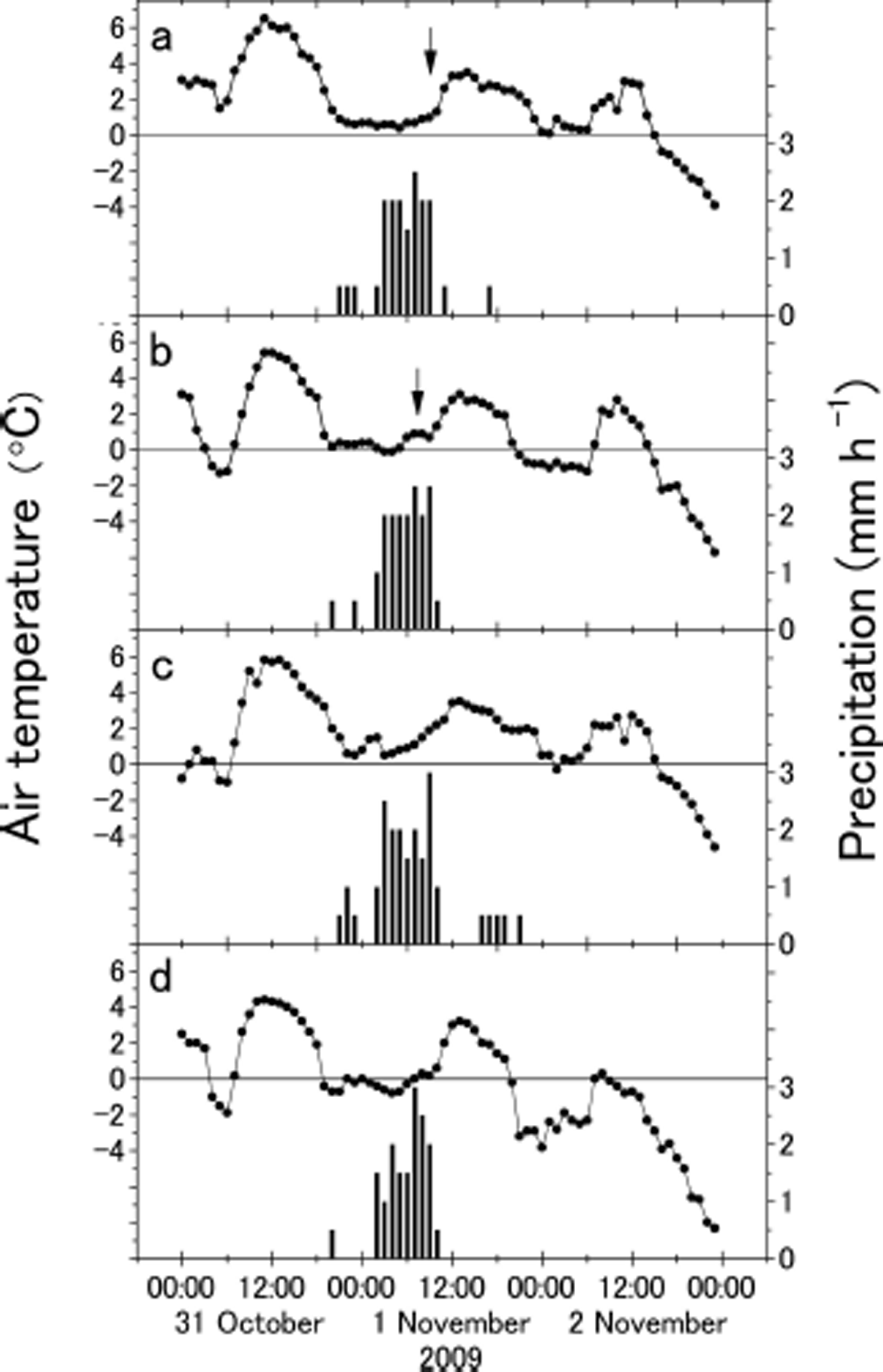
Since the Kitami AMeDAS site is only ~3 km west of where white spotted wet snow was observed in Kitami, we assumed that meteorological conditions at both sites were almost the same. As shown in Figure 5a, in Kitami, precipitation was recorded from 21:00 on 31 October to 09:00 on 1 November, but not from 00:00 to 01:00. Total precipitation during this period was 16.0 mm. Precipitation conditions in Kitami, Oketo, Bihoro and Rubeshibe were similar (Fig. 5a–d). Air temperature during this period in Kitami ranged from 0.4 to 1.0°C, and average air temperature was 0.7°C. Thus, most of the precipitation was supplied as snow or ice pellets. Average wind speed in Kitami from 21:00 on 31 October to 09:00 on 1 November was 0.9 m s^–1, with calm wind conditions (wind speed = 0) recorded from 02:00 to 06:00 on 1 November.

Figure 5b shows meteorological conditions in Oketo. Air temperature in Oketo from 21:00 on 31 October to 09:00 on 1 November ranged from –0.1 to 0.9°C, and average air temperature was 0.4°C, similar to temperature conditions in Kitami. Figure 5c shows meteorological conditions in Bihoro. Air temperature in Bihoro during the same interval ranged from 0.5 to 1.9°C, with an average of 1.0°C, higher than in Kitami or Oketo. Figure 5d shows meteorological conditions in Rubeshibe. Air temperature in Rubeshibe during the same interval ranged from –0.8 to 0.3°C, and average air temperature was –0.3°C, lower than in Kitami or Oketo.

As described in Section 2, white spotted wet snow was not observed in Bihoro or Rubeshibe. It did not form in Bihoro probably because the ice and snow grains in the mixed ice–water layer on the asphalt road in Bihoro melted. In Rubeshibe, the surface of the mixed ice–water layer probably froze and formed a thin ice layer, so white spotted wet snow did not form.

4. Process Of White Spot Formation

Figure 6 shows a schematic diagram of the process of white spotted wet snow formation. The surface temperature of the asphalt pavement in Kitami when the snow fell at 21:00 on 31 October (Fig. 6a) is unknown. However, the temperature was probably above the melting point because of the relatively warm conditions in the daytime (average daily temperatures on 31 October were 3.5°C in Kitami and 2.0°C in Oketo). Thus, snow melted on the road and formed wet snow (Fig. 6b). When snow melts on a surface, the surface snow layer becomes impermeable to air (Fig. 6c). In this case, the void volumes in the wet snow became small air bubbles (Fig. 6d). These air bubbles coalesced and formed air bubbles 10–100 mm in diameter (Fig. 6e). Consequently, the air in the bubbles was supplied from the void volume in the wet snow. When the wet snow was deeper, the diameter of the air bubbles was larger, as was the case in Oketo (Fig. 4).

Fig. 6.

Schematic diagram of the formation of white spotted wet snow.

The coalescing process of small air bubbles (Fig. 6d) into large air bubbles (Fig. 6e) is important to form white spotted wet snow. Properties of water and air, especially surface tensions and viscosities of water and air, will be the key factors for the process.

5. White Spot Statistics

5.1. Number density and diameter of white spots

The horizontal distribution of white spots in a 97.5 cm × 73.0 cm area in Kitami is shown in Figure 7a. White spots, ice grains that were not soaked in water and small stones that were present in the asphalt road are shown in Figure 7a. Because the ice grains were <1 mm in diameter and most of the small stones were <8 mm in diameter, we counted only white spots >8 mm in diameter. As a result, we counted 69 white spots in Figure 7a, of which six were at the edge of the figure. Using image analysis software (Image-Pro Plus, Nippon Rover, Inc.), the boundaries and the gravitational centre of the white spots were examined.

Fig. 7.

(a) Horizontal distribution of white spots (taken at Kitami at 09:00, 1 November 2009). (b) Nearest distances for L series white spots are shown as straight lines. (c) Nearest distances from S to L series white spots are shown as straight lines. The periphery and gravitational centre of the white spots are shown with lines and dots, respectively.

Figure 8 shows the distribution of the diameters of the white spots shown in Figure 7a. The spots were divided into two categories: ≥15 mm in diameter (L series) and <15 mm (S series). The shape of an L series white spot was similar to a circle, while the shape of an S series white spot was indeterminate. Table 1 summarizes these statistics. The total area of L and S series white spots was 540.2 cm², which represents 7.6% of the observed area (7117.5 cm², 97.5 cm × 73.0 cm) in Figure 7a.

Fig. 8.

Distribution of the diameter of white spots in Figure 7a.

Table 1.

Number, diameter and areas of the white spots shown in Figure 7a

5.2. Horizontal distribution of white spots

5.2.1. Analysis by nearest-neighbour method

The nearest-neighbour method calculates the nearest distances between points that are distributed on a horizontal surface. By comparison to the average distance of randomly distributed points, we can estimate the regularity of their distribution (Reference RipleyRipley, 1981). The method was originally developed for estimating the distribution of trees in a field (Reference Clark and EvansClark and Evans, 1954) and is used mainly in the disciplines of ecology and geography (e.g. Reference LeeLee, 1979).

The average nearest distance for L series white spots is calculated by Eqn (1). We used the gravitational centre of each white spot. The value of d _Li is the nearest distance of an L series white spot and n is the number of L series white spots. The average nearest distance between L and S series white spots was calculated from Eqn (2). The value of d _LSi is the nearest distance from an L series to an S series white spot, d _SLj is the nearest distance from an S series to an L series white spot, m is the number of S series white spots, and N is equal to n + m.

(1)

(2)

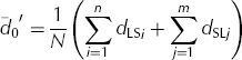
Figure 7b shows the nearest distances for L series white spots using straight lines, and Figure 7c shows the nearest distances between L and S series white spots using straight lines. The six L series white spots located at the edge of Figure 7a were discounted in the calculations using Eqns (1) and (2) because of the ‘edge effects’ described by Reference RipleyRipley (1981).

If the white spots are randomly distributed, the average nearest distance d _E is given by Eqn (3). The nearest distance value R is calculated using Eqn (4).

(3)

(4)

Here A is the observational area. If the spots are distributed randomly, R will be 1. If the spots are distributed with a hexagonal distribution, R will be 2.149. This is the maximum possible value for R. If the spots exist in only one position, R will be 0.

Using the 47 L series white spots in Figure 6a, the d ₀ was 93.9 mm and the d _E was 65.1 mm. Thus, R was 1.44. This indicated that the L series white spots were not randomly distributed, but were regularly distributed at some level. The difference between 1.44 and 1 was examined using the Z score (Reference SugiuraSugiura, 2003) given by

(5)

(6)

The Z value, 5.48, is larger than the significance value at 0.1% (Z _0.001 = 3.291). Thus, we considered that L series white spots were not randomly distributed.

Equation (7) gives the nearest distance at which L series and S series white spots were randomly distributed, and the value of R’ indicates the distribution between L series and S series white spots.

(7)

(8)

Here n _L is the ratio of L series white spots to the total number of white spots (n _L = n/N), and m _S is the ratio of S series white spots to the total number of white spots (m _S = m/N). If L series white spots and S series white spots are randomly distributed, R’ will be 1. If L series white spots and S series white spots are distributed at only one point, R ^’ will be 0. If all L series white spots are located on S series white spots, R ^’ will be 0.

Using Eqns (2) and (7), d ₀ ^’ was 98.2 mm and d _E was 75.0 mm, and thus R ^; was 1.31. This means that S series white spots were not randomly distributed. In other words, S series white spots were distributed close to L series white spots at some level. The difference between 1.31 and 1 was examined using the Z score (Reference SugiuraSugiura, 2003) given by

(9)

(10)

(11)

The Z value comes to 5.14, larger than the significance value at 0.1% (Z _0.001 = 3.291). Thus, we considered that S series white spots were not randomly distributed.

5.2.2. Analysis using a Voronoi diagram

A Voronoi diagram consists of a polygon calculated using the perpendicular bisectors of two points (e.g. Okabe and others, 2000; Reference SugiharaSugihara, 2009). We used the gravitational centre of each white spot for calculations using computer software (Voronoi partition.exe). Figure 9a shows the boundaries and gravitational centres of all the white spots in Figure 7a, and Figure 9b shows a Voronoi diagram of the L series white spots. Each domain in Figure 9b corresponds to an air-captured area of L series white spots from the definition of a Voronoi diagram. Figure 10 shows the number of sides in the polygons in Figure 9b. We excluded the polygons that faced the edges. We found that the number of hexagonal polygons was higher than the number of other types. This suggests that a white spot in Figure 7a tends to be surrounded by six other white spots.

Fig. 9.

(a) Periphery and gravitational centre of the white spots. (b) Voronoi diagram; lines are the perpendicular bisectors of two points.

Fig. 10.

Frequency distribution of the number of lines in a Voronoi diagram, shown in Figure 9b.

On the other hand, Reference Kumar and KurtzKumar and Kurtz (1993) clarify that a Voronoi tessellation of a Poisson point process, i.e. a random distribution, has the maximum probability at hexagonal polygons using a Monte Carlo simulation of 2 × 10⁶ polygons. Because the white spots in Figure 7a were not randomly distributed (Section 5.2.1), we consider that analytical results in Figure 10 reflect the true nature of the horizontal distribution of white spots.

5.2.3. Analysis by the two-dimensional (2-D) correlation function

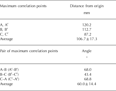
A normalized autocorrelation function was used for analysing periodicity in the horizontal distribution of white spots. The 2-D normalized correlation is defined by (Reference BracewellBracewell, 2000; Reference TakaiTakai, 2000)

(12)

where x and y are rectangular coordinates, u (x, y) is an image, and Δx and Δy are displacements of the image. The calculations were performed by an image analysis program produced by MATLAB^® (The MathWorks, Inc.) using the Wiener–Khintchine formulae (Reference HinoHino, 1977; Reference TakaiTakai, 2000). Figure 11 shows the distribution of the normalized correlation for a displacement of 300 mm in the x – and y –axes using the above calculations. Maximum correlation areas were labelled A–E, and symmetrical positions were labelled A’-E’. We found that six areas with high correlation values (A–C) exist around the origin of the coordinates. Table 2 shows the distance from the centre and the angles between the two areas. Each distance ranged from 87.2 to 120.2 mm and the angles ranged from 43° to 68°. The average values ± the standard deviation were 106.7 ± 17.3 mm and 60.0 ± 14.4°, respectively. This result demonstrates that one white spot tends to be surrounded by six other spots.

Fig. 11.

Distribution of the 2-D normalized correlation of the white spots in Figure 7a. High-correlation areas are labelled A–E and their symmetrical positions are labelled A′–E′.

Table 2.

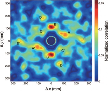
Distances and angles for the maximum correlation areas (A–C, A^’–C^’) shown in Figure 11

Using three independent methods, we found that white spots were not randomly distributed, and that one white spot tends to be surrounded by six other spots. This can be explained by the hexagonal close-packed (hcp) structure having the highest packing ratio (74%, = π/(3√2)) for equal-radius circles in a horizontal surface (Fig. 12). Because the white spots are formed by air trapped in the mixed ice–water layer, the positions of the spots are determined by competition between these air bubbles in the layer. These characteristics of white spotted wet snow were also verified by other observations of white spotted wet snow in the 2010/11 winter, which will be reported elsewhere.

Fig. 12.

Hexagonal close-packed (hcp) structure for equal-radius circles on a horizontal surface. The unit cell of a triangle is shown with a bold line.

6. Conclusions

This paper summarizes observations of white spotted wet snow in Kitami and Oketo on 1 November 2009. The main results of this study are:

1. 1. White spotted wet snow was formed on an asphalt road, concrete, and tile pavements in Kitami and Oketo, eastern Hokkaido. These materials are almost impermeable to water.

2. 2. A thin water layer 2–5 mm thick existed just above the road. A mixed ice–water layer 2–3 mm thick existed on the thin water layer. Ice grains 1 mm in diameter and small snow grains were present in the mixed ice–water layer.

3. 3. Thin air bubbles ~1 mm thick were present between the thin water layer and the mixed ice–water layer, and formed white spots due to the diffusive reflection of sunlight between the two layers.

4. 4. We considered the process of white spotted wet snow formation using meteorological data in Kitami. The impermeable surface layer of wet snow was important for the formation of white spotted wet snow.

5. 5. Large and small white spots were not randomly distributed. We found that one large white spot tends to be surrounded by six other large white spots. In general, hexagonal close packing (hcp) had the highest packing ratio for equal-radius circles on a horizontal surface. This is the reason for the observed results.

Our results indicate that white spots form on impermeable materials with a 10–30 mm thickness of water-saturated snow. When a small amount of snow is deposited on glacier or sea ice, and the snow is partially melted by solar radiation or positive temperatures, the above conditions are easily satisfied. Thus, we consider that white spotted wet snow probably forms on glacier ice or sea ice. However, as both the ice and the spots are white, it will be difficult to identify white spots on ice.

According to our observations, the diameter of the white spots ranged from 30 to 100 mm. The physics controlling the coalescing process of air bubbles (Fig. 6d–e) will be our next target in our studies of ‘white spots physics’.