


1. Introduction
The chain-ladder algorithm to compute the unpaid claim requirement in an insurance financial statement is the most well-known reservation methodology in actuarial practice. This algorithm has been widely examined by many researchers in the last three decades, such as Kremer (Reference Kremer1982), Taylor (Reference Taylor1986, Reference Taylor2000), Renshaw (Reference Renshaw1989), Verrall (Reference Verrall1990), Mack (Reference Mack1993), Murphy (Reference Murphy1994), Schmidt & Schnaus (Reference Schmidt and Schnaus1996), Barnett & Zehnwirth (Reference Barnett and Zehnwirth1998), England & Verrall (Reference England and Verrall1999) and Wüthrich & Merz (Reference Wüthrich and Merz2008).
In particular, considerable research related to the well-known distribution-free chain-ladder model by Mack has been performed. In terms of the prediction uncertainty estimation within Mack’s model, the most relevant contributions include those of Mack (Reference Mack1993), Buchwalder et al., (Reference Buchwalder, Bühlmann, Merz and Wüthrich2006), Mack et al., (Reference Mack, Quarg and Braun2006), Gisler (Reference Gisler2006, Reference Gisler2019, Reference Gisler2020), Merz & Wüthrich (Reference Merz and Wüthrich2008, Reference Merz and Wüthrich2014), Röhr (Reference Röhr2016), England et al., (Reference England, Verrall and Wüthrich2019), Diers et al., (Reference Diers, Linde and Hahn2016) and Lindholm et al., (Reference Lindholm, Lindskog and Wahl2020).
In 1993, Mack derived an estimator (Mack formula) to quantify the ultimate prediction uncertainty within his model. Later, in 2006, certain controversial discussions occurred (see Mack et al., Reference Mack, Quarg and Braun2006; Gisler Reference Gisler2006) when Buchwalder et al., (Reference Buchwalder, Bühlmann, Merz and Wüthrich2006) proposed a novel estimator (BBMW formula); however, the question related to which of the two formulas should be preferred went unanswered. Recently, Gisler (Reference Gisler2020) stated that the Mack formula should be preferred over the BBMW formula. Notably, Gisler (Reference Gisler2020) highlighted several deficiencies related to the BBMW estimator, linked with the conditional resampling approach, which was adopted in Buchwalder et al., (Reference Buchwalder, Bühlmann, Merz and Wüthrich2006) to derive the estimator for the second term of the conditional mean squared error of prediction (MSEP), usually known as the estimation error. Moreover, Gisler (Reference Gisler2020) proved that for individual accident years, the Mack estimator of the estimation error does (on average, given partial information) overestimates the true prediction uncertainty, albeit to a smaller extent than the BBMW estimator.
However, Gisler (Reference Gisler2019) previously demonstrated that the Mack formula can be derived by applying a certain estimation principle, that is unfortunately, as mentioned in the original article, not fully well-defined and must be applied with caution especially when non-linear functions in the unknown parameters need to be estimated.
Considering these aspects and principally the fact that both Mack and BBMW formulas result to be biased (as demonstrated in Gisler Reference Gisler2020), in this paper, we propose a new estimator for the ultimate prediction uncertainty within the famous Mack’s distribution-free chain-ladder model, which under some additional technical assumptions can be proved to be unbiased.
Unluckily, the new unbiased estimator does show some peculiar behaviours, in particular with respect to its possible negativity. This is a drawback which might be worth trading off for the unbiasedness property, since there is empirical evidence that the likelihood of a negative realisation is extremely low.
Organisation of the paper. In section 2, we specify the model assumptions of the Mack chain-ladder model and recall the traditional notation as well as some key results. Moreover, we define the true value of the ultimate claim prediction uncertainty for both single accident years and for the total over all accident years.
In section 3, we propose a novel formula which can be used as an estimator for the true uncertainty and can be demonstrated to be conditionally unbiased given the first triangle column.
In section 4, we consider several numerical examples to compare the results from the different formulas and demonstrate that both the Mack and BBMW formulas as well as the new formula can (with non-negligible probability) materially fail to predict the true uncertainty.
2. Mack Model
As usual in claims reserving, we denote by $C_{i,\,j}>0$
the cumulative claim figures from accident years
$C_{i,\,j}>0$
the cumulative claim figures from accident years $i \in \{0,\dots,I\}$
at the end of development years
$i \in \{0,\dots,I\}$
at the end of development years $j \in \{0,\dots,J\}, \, J \le I$
and we assume that the claims are fully developed at the end of development year J.
$j \in \{0,\dots,J\}, \, J \le I$
and we assume that the claims are fully developed at the end of development year J.
For time $t \in \{0,\dots,I+J\}$
,
$t \in \{0,\dots,I+J\}$
, $\mathcal{D}_{t}$
indicates the cumulative claims payment data
$\mathcal{D}_{t}$
indicates the cumulative claims payment data $(C_{i,\,j})$
up to time t. For instance, at time I we have
$(C_{i,\,j})$
up to time t. For instance, at time I we have
 \begin{align}\mathcal{D}_{I}=\left\{C_{i,\,j}\;:\; i=0,\dots,I, \, i+j \le I\right\}.\end{align}
In 1993, the following distribution-free stochastic model underlying the chain-ladder reserving method was introduced by Mack (Reference Mack1993).
Model Assumptions 1 (Mack model).
-
• Vectors $(C_{i,\,0},\dots,C_{i,\,J})$
,
$\,i \in \{0,\dots,I\}$
are independent
$(C_{i,\,0},\dots,C_{i,\,J})$
,
$\,i \in \{0,\dots,I\}$
are independent -
• There exist positive parameters
$f_0,\dots,f_{J-1}$
and
$\sigma_0^2,\dots,\sigma_{J-1}^2$
such that for all
$i \in \{0,\dots,I\}$
and all
$j \in \{0,\dots,J-1\}$
(2)
\begin{align} E[C_{i,\,j+1}|C_{i,\,0},\dots,C_{i,\,j}]=f_j C_{i,\,j}, \end{align}
(3)
\begin{align} Var(C_{i,\,j+1}|C_{i,\,0},\dots,C_{i,\,j})=\sigma_j^2 C_{i,\,j}. \end{align}


Within Mack’s model, the unknown parameters $f_0,\dots,f_{J-1}$
and
$f_0,\dots,f_{J-1}$
and $\sigma_0^2,\dots,\sigma_{J-1}^2$
are estimated at time I by using the following, conditionally given
$\sigma_0^2,\dots,\sigma_{J-1}^2$
are estimated at time I by using the following, conditionally given $\mathcal{B}_{j}=\{ C_{i,\,k}; i+k \le I, k\le j\} \subset \mathcal{D}_I$
, unbiased estimators
$\mathcal{B}_{j}=\{ C_{i,\,k}; i+k \le I, k\le j\} \subset \mathcal{D}_I$
, unbiased estimators
 \begin{align} \widehat{f_j}&=\frac{\sum_{i=0}^{I-j-1}C_{i,\,j+1}}{\sum_{i=0}^{I-j-1} C_{i,\,j}},\quad j\in \{0,\dots,J-1\},\end{align}
 \begin{align} \widehat{\sigma_j^2}&=\frac{1}{I-j-1}\sum_{i=0}^{I-j-1} C_{i,\,j}\left(\frac{C_{i,\,j+1}}{C_{i,\,j}}-\widehat{f_j}\right)^2,\quad j\in \{0,\dots,J-1\}, \end{align}
where, for $J=I$
,
$J=I$
, $\sigma_{J-1}^2$
is usually estimated through extrapolation as
$\sigma_{J-1}^2$
is usually estimated through extrapolation as
 \begin{align}\widehat{\sigma_{J-1}^2}&=\min\left(\widehat{\sigma_{J-3}^2},\widehat{\sigma_{J-2}^2},\frac{\left(\widehat{\sigma_{J-2}^2}\right)^2}{\widehat{\sigma_{J-3}^2}}\right).\end{align}
The ultimate claim $C_{i,\,J}$
for accident year
$C_{i,\,J}$
for accident year $i \in \{0,\dots,I\}$
is at time I predicted by
$i \in \{0,\dots,I\}$
is at time I predicted by
 \begin{align} \widehat{C}_{i,J}=C_{i,\,I-i} \prod_{j=I-i}^{J-1} \widehat{f}_j.\end{align}
Predictor (7) is, conditionally given $\mathcal{B}_{I-i}$
, unbiased for
$\mathcal{B}_{I-i}$
, unbiased for $E\left[C_{i,\,J}\big|\mathcal{B}_{I-i}\right]=E\left[C_{i,\,J}\big|\mathcal{D}_I\right]$
, i.e. we have
$E\left[C_{i,\,J}\big|\mathcal{B}_{I-i}\right]=E\left[C_{i,\,J}\big|\mathcal{D}_I\right]$
, i.e. we have
 \begin{align}E\left[\widehat{C}_{i,J}\big|\mathcal{B}_{I-i}\right]=E\left[C_{i,\,J}\big|\mathcal{B}_{I-i}\right].\end{align}
Moreover, the ultimate claim $\sum_{i=0}^I C_{i,\,J}$
for the total over all accident years is at time I predicted by
$\sum_{i=0}^I C_{i,\,J}$
for the total over all accident years is at time I predicted by
 \begin{align} \sum_{i=0}^I \widehat{C}_{i,J}.\end{align}
Predictor (9) is, conditionally given $\mathcal{B}_{0}$
, unbiased for
$\mathcal{B}_{0}$
, unbiased for $E\left[\sum_{i=0}^I C_{i,\,J}\big|\mathcal{B}_{0}\right]$
, i.e. we have
$E\left[\sum_{i=0}^I C_{i,\,J}\big|\mathcal{B}_{0}\right]$
, i.e. we have
 \begin{align}E\left[\sum_{i=0}^I \widehat{C}_{i,J}\bigg|\mathcal{B}_{0}\right]=E\left[\sum_{i=0}^I C_{i,\,J}\bigg|\mathcal{B}_{0}\right].\end{align}
Furthermore, Mack (Reference Mack1993) also demonstrated that it holds true
 \begin{align} E\left[\left(\widehat{f}_j\right)^2\bigg|\mathcal{B}_j\right]=f_j^2+\frac{\sigma^2_j}{\sum_{h=0}^{I-j-1}C_{h,j}},\quad j\in \{0,\dots,J-1\}. \end{align}
2.1 Quantification of the ultimate claim prediction error
The objective is to quantify the ultimate claim prediction uncertainty at time I for both single and aggregated accident years. In a distribution-free framework, this is usually done by considering the following quantities of interest which will be also referred to as the true values, because they measure, with respect to the squared loss function, the expected deviation between the unknown ultimate claim amounts ( $C_{i,\,J}$
and
$C_{i,\,J}$
and $\sum_{i=0}^I C_{i,\,J}$
respectively) and their predicted amounts (
$\sum_{i=0}^I C_{i,\,J}$
respectively) and their predicted amounts ( $\widehat{C}_{i,J}$
and
$\widehat{C}_{i,J}$
and $\sum_{i=0}^I\widehat{C}_{i,J,}$
respectively) at time I.
$\sum_{i=0}^I\widehat{C}_{i,J,}$
respectively) at time I.
Definition 1 (Conditional MSEP for single accident years). The conditional MSEP of the ultimate claim predictor for single accident year i is defined as
 \begin{align} {\rm msep}_{C_{i,\,J}|\mathcal{D}_I}\left(\widehat{C}_{i,J}\right)&=E\left[\left(C_{i,\,J}-\widehat{C}_{i,J}\right)^2\bigg|\mathcal{D}_I\right].\end{align}
The true value (12) can be decomposed as follows:
 \begin{align} {\rm msep}_{ C_{i,\,J}|\mathcal{D}_I}\left(\widehat{C}_{i,J}\right)&=Var\left(C_{i,\,J}\bigg|\mathcal{D}_I\right)+ \left( \widehat{C}_{i,J} -E\left[ C_{i,\,J}\bigg|\mathcal{D}_I\right]\right)^2 \nonumber\\[5pt] &=\underbrace{ Var\left(C_{i,\,J}\bigg|\mathcal{D}_I\right)}_{\textrm{PV}_{i}}+ \underbrace{C_{i,\,I-i}^2 \left(\prod_{j=I-i}^{J-1} \widehat{f}_j - \prod_{j=I-i}^{J-1} f_j \right)^2}_{\textrm{EE}_{i}},\end{align}
where $\textrm{PV}_{i}$
denotes the process variance and
$\textrm{PV}_{i}$
denotes the process variance and $\textrm{EE}_{i}$
the estimation error of an individual accident year i.
$\textrm{EE}_{i}$
the estimation error of an individual accident year i.
Definition 2 (Conditional MSEP for aggregated accident years). The conditional MSEP of the ultimate claim predictor for aggregated accident years is defined as
 \begin{align} {\rm msep}_{\sum_{i=0}^I C_{i,\,J}|\mathcal{D}_I}\left(\sum_{i=0}^I \widehat{C}_{i,J}\right)&=E\left[\left(\sum_{i=0}^I (C_{i,\,J}-\widehat{C}_{i,J})\right)^2\bigg|\mathcal{D}_I\right].\end{align}
The true value (14) can be decomposed as follows:
 \begin{align} {\rm msep}_{\sum_{i=0}^I C_{i,\,J}|\mathcal{D}_I}\left(\sum_{i=0}^I \widehat{C}_{i,J}\right)&=Var\left(\sum_{i=0}^I C_{i,\,J}\bigg|\mathcal{D}_I\right)+ \left(\sum_{i=0}^I \widehat{C}_{i,J} -E\left[\sum_{i=0}^I C_{i,\,J}\bigg|\mathcal{D}_I\right]\right)^2 \nonumber\\[5pt] &=\underbrace{\sum_{i=0}^I Var\left(C_{i,\,J}\bigg|\mathcal{D}_I\right)}_{\sum_{i=0}^I\textrm{PV}_{i}=\textrm{PV}_{\textrm{tot}}}+ \underbrace{\left(\sum_{i=0}^I C_{i,\,I-i} \left(\prod_{j=I-i}^{J-1} \widehat{f}_j - \prod_{j=I-i}^{J-1} f_j \right)\right)^2}_{\textrm{EE}_{\textrm{tot}}},\end{align}
where $\textrm{PV}_\textrm{tot}$
denotes the process variance for the total over all accident years and
$\textrm{PV}_\textrm{tot}$
denotes the process variance for the total over all accident years and $\textrm{EE}_{\textrm{tot}}$
the estimation error for the total over all accident years.
$\textrm{EE}_{\textrm{tot}}$
the estimation error for the total over all accident years.
The process variance $\textrm{PV}_{i}$
can be easily calculated. By iteration, the Model Assumptions 1 indicate that (see Mack, Reference Mack1993)
$\textrm{PV}_{i}$
can be easily calculated. By iteration, the Model Assumptions 1 indicate that (see Mack, Reference Mack1993)
 \begin{align} \textrm{PV}_{i}= C_{i,\,I-i} \sum_{k=I-i}^{J-1} \left(\prod_{m=I-i}^{k-1} f_m \right) \sigma_k^2 \left(\prod_{n=k+1}^{J-1} f_n^2\right), \quad i \in \{0,\dots,I\}.\end{align}
On the other side, the estimation errors (for single accident year i and for the total over all accident years) can be easily expressed as
 \begin{align} &\textrm{EE}_{i}= C_{i,\,I-i}^2\left(\prod_{k=I-i}^{J-1} \left(\widehat{f}_k\right)^2+\prod_{k=I-i}^{J-1} f_k^2 -2\prod_{k=I-i}^{J-1} f_k \widehat{f}_k\right), \quad i \in \{0,\dots,I\},\end{align}
 \begin{align} &\textrm{EE}_{\textrm{tot}}=\sum_{i=1}^I \textrm{EE}_{i} +2\sum_{1 \le i<j\le I} C_{i,\,I-i}C_{j,I-j} \left(\prod_{k=I-i}^{J-1} \widehat{f}_k - \prod_{k=I-i}^{J-1} f_k \right)\left(\prod_{k=I-j}^{J-1} \widehat{f}_k - \prod_{k=I-j}^{J-1} f_k \right).\end{align}
3. The New Formula
Since the model parameter $(f_{j})$
and
$(f_{j})$
and $(\sigma_j^2)$
are unknown, the true value (12) given by
$(\sigma_j^2)$
are unknown, the true value (12) given by $\textrm{PV}_{i}+\textrm{EE}_{i}$
cannot be evaluated. For the process variance, the traditional approach in actuarial literature considers the estimator (19) for
$\textrm{PV}_{i}+\textrm{EE}_{i}$
cannot be evaluated. For the process variance, the traditional approach in actuarial literature considers the estimator (19) for $\textrm{PV}_{i}$
based on the data
$\textrm{PV}_{i}$
based on the data $\mathcal{D}_{I}$
(see Mack, Reference Mack1993):
$\mathcal{D}_{I}$
(see Mack, Reference Mack1993):
 \begin{align} \widehat{\textrm{PV}_{i}}^{\textrm{Mack}}&=\sum_{k=I-i}^{J-1} C_{i,\,I-i} \left(\prod_{m=I-i}^{k-1} \widehat{f}_m\right)\widehat{\sigma_k^2}\prod_{n=k+1}^{J-1} \left(\widehat{f}_n\right)^2.\end{align}
But unfortunately, this proposal does not result to be, conditionally given $\mathcal{B}_{I-i}$
, unbiased for
$\mathcal{B}_{I-i}$
, unbiased for $E\left[\textrm{PV}_{i}\big|\mathcal{B}_{I-i}\right]$
.
$E\left[\textrm{PV}_{i}\big|\mathcal{B}_{I-i}\right]$
.
On the other hand, for the estimation error, the traditional approach focus on estimating $E\left[\textrm{EE}_{i}\big|\mathcal{B}_{I-i}\right]$
based on the data
$E\left[\textrm{EE}_{i}\big|\mathcal{B}_{I-i}\right]$
based on the data $\mathcal{D}_{I}$
, since directly estimating the positive term
$\mathcal{D}_{I}$
, since directly estimating the positive term $\textrm{EE}_{i}$
based on the data
$\textrm{EE}_{i}$
based on the data $\mathcal{D}_{I}$
leads to a degenerated estimator (namely 0).
$\mathcal{D}_{I}$
leads to a degenerated estimator (namely 0).
However, the until now known proposals (see Mack, Reference Mack1993 and Buchwalder et al., Reference Buchwalder, Bühlmann, Merz and Wüthrich2006) do not result to be, conditionally given $\mathcal{B}_{I-i}$
, unbiased for
$\mathcal{B}_{I-i}$
, unbiased for $E\left[\textrm{EE}_{i}\big|\mathcal{B}_{I-i}\right]$
(see Gisler, Reference Gisler2020).
$E\left[\textrm{EE}_{i}\big|\mathcal{B}_{I-i}\right]$
(see Gisler, Reference Gisler2020).
3.1 Single accident years
In this paper, our goal is to derive estimators $\widehat{\textrm{PV}_{i}}^{\textrm{NEW}}$
and
$\widehat{\textrm{PV}_{i}}^{\textrm{NEW}}$
and $\widehat{\textrm{EE}_{i}}^{\textrm{NEW}}$
that fulfil the properties
$\widehat{\textrm{EE}_{i}}^{\textrm{NEW}}$
that fulfil the properties
 \begin{align} E\left[\widehat{\textrm{PV}_{i}}^{\textrm{NEW}}\bigg|\mathcal{B}_{I-i}\right]=E\left[\textrm{PV}_{i} \bigg|\mathcal{B}_{I-i}\right]< \infty,\end{align}
and
 \begin{align} E\left[\widehat{\textrm{EE}_{i}}^{\textrm{NEW}}\bigg|\mathcal{B}_{I-i}\right]=E\left[\textrm{EE}_{i}\bigg|\mathcal{B}_{I-i}\right]< \infty,\end{align}
i.e. estimators which result to be, conditionally given $\mathcal{B}_{I-i}$
, unbiased for
$\mathcal{B}_{I-i}$
, unbiased for $E\left[\textrm{PV}_{i} \big|\mathcal{B}_{I-i}\right]$
and
$E\left[\textrm{PV}_{i} \big|\mathcal{B}_{I-i}\right]$
and $E\left[\textrm{EE}_{i} \big|\mathcal{B}_{I-i}\right]$
respectively.
$E\left[\textrm{EE}_{i} \big|\mathcal{B}_{I-i}\right]$
respectively.
Let us first present a, conditionally given $\mathcal{B}_{I-i}$
, unbiased estimator for
$\mathcal{B}_{I-i}$
, unbiased estimator for $\prod_{k=I-i}^{J-1} f_k^2$
.
$\prod_{k=I-i}^{J-1} f_k^2$
.
We have the following Theorem.
Theorem 1. Provided $E\left[\bigg|\prod_{j=I-i}^{J-1}\left(\left(\widehat{f}_j\right)^2 -\frac{\widehat{\sigma_j^2}}{\sum_{k=0}^{I-j-1} C_{k,j}}\right)\bigg|\right] < \infty$
, under Model Assumptions 1 (with
$E\left[\bigg|\prod_{j=I-i}^{J-1}\left(\left(\widehat{f}_j\right)^2 -\frac{\widehat{\sigma_j^2}}{\sum_{k=0}^{I-j-1} C_{k,j}}\right)\bigg|\right] < \infty$
, under Model Assumptions 1 (with $J<I$
) we have that the estimator
$J<I$
) we have that the estimator
 \begin{align} \prod_{j=I-i}^{J-1}\left(\left(\widehat{f}_j\right)^2 -\frac{\widehat{\sigma_j^2}}{\sum_{k=0}^{I-j-1} C_{k,j}}\right), \quad i \in \{I-J+1,\dots,I\},\end{align}
is, conditionally given $\mathcal{B}_{I-i}$
, unbiased for
$\mathcal{B}_{I-i}$
, unbiased for $\prod_{j=I-i}^{J-1} f_j^2$
.
$\prod_{j=I-i}^{J-1} f_j^2$
.
Proof. From result (11) as well as the conditionally unbiasedness of the parameter estimates ( $\widehat{\sigma_j^2}$
), we get
$\widehat{\sigma_j^2}$
), we get
 \begin{align}\!\!\!\!\!\!\!\!\!\!\!\!\!\!\!\!\!\!\!\!\!\!\!\!\!\!\!\!\!\!\!\!\!\!\!\!\!\!\!\!\!\!\!\!\!\!\!\!\!\!\!\!\!\!\!\!\!\!\!\!\!\!\!\!\!\!\infty > E\left[\prod_{j=I-i}^{J-1}\left(\left(\widehat{f}_j\right)^2 -\frac{\widehat{\sigma_j^2}}{\sum_{k=0}^{I-j-1} C_{k,j}}\right)\bigg|\mathcal{B}_{I-i} \right]\qquad\quad\qquad \nonumber \end{align}
 \begin{align} & \quad = E\left[E\left[\prod_{j=I-i}^{J-1}\left(\left(\widehat{f}_j\right)^2 -\frac{\widehat{\sigma_j^2}}{\sum_{k=0}^{I-j-1} C_{k,j}}\right)\bigg|\mathcal{B}_{J-1} \right]\bigg|\mathcal{B}_{I-i} \right]\nonumber\\[5pt] & \quad =E\left[\prod_{j=I-i}^{J-2}\left(\left(\widehat{f}_j\right)^2 -\frac{\widehat{\sigma_j^2}}{\sum_{k=0}^{I-j-1} C_{k,j}}\right)E\left[\left(\widehat{f}_{J-1}\right)^2 -\frac{\widehat{\sigma_{J-1}^2}}{\sum_{k=0}^{I-J} C_{k,{J-1}}}\bigg|\mathcal{B}_{J-1} \right]\bigg|\mathcal{B}_{I-i} \right]\nonumber\\[5pt]& \quad =E\left[\prod_{j=I-i}^{J-2}\left(\left(\widehat{f}_j\right)^2 -\frac{\widehat{\sigma_j^2}}{\sum_{k=0}^{I-j-1} C_{k,j}}\right)\bigg|\mathcal{B}_{I-i} \right] f^2_{J-1}=\ldots=\prod_{j=I-i}^{J-1} f_j^2, \quad i \in \{I-J+1,\dots,I\}.\nonumber\end{align}
In order to guarantee the existence of the involved quantities, in the following we will work under the additional technical assumptions
 \begin{align} E\left[\prod_{j=I-i}^{J-1}\left(\widehat{f}_j\right)^2\right] < \infty, \quad i \in \{I-J+1,\dots,I\},\end{align}
and
 \begin{align} E\left[\bigg|\prod_{j=I-i}^{J-1}\left(\left(\widehat{f}_j\right)^2 -\frac{\widehat{\sigma_j^2}}{\sum_{k=0}^{I-j-1} C_{k,j}}\right)\bigg|\right] < \infty, \quad i \in \{I-J+1,\dots,I\}.\end{align}
Remark 1. As not uncommonly, the technical assumptions (23) and (24) are unverifiable. However, they can be reasonably assumed to hold true, since they are consistent with data typically encountered in actuarial practice. Moreover, we underline that the core technical requirement for the unbiasedness result stated in Theorem 1 is the technical assumption (24) and not the positivity of estimator (22) along all the possible trajectories.
Under Model Assumptions 1 and the technical assumption (24), there could exist trajectories of the underlying claims payments process for which the realisations of estimator (22) are negative. This is a drawback of the unbiased estimator (22) but not a probabilistic issue, since estimators are random variables, and their realisations may even significantly differ from the quantity they intend to estimate. However, for typical general insurance data, the unbiased estimator (22) results to be positive. This is due to the fact that for typical data, the term $\left(\widehat{f}_j\right)^2$
dominates
$\left(\widehat{f}_j\right)^2$
dominates $\frac{\widehat{\sigma_j^2}}{\sum_{h=0}^{I-j-1}C_{h,j}}$
. This is also the argument that justifies the common use of the first-order Taylor approximations in this domain.
$\frac{\widehat{\sigma_j^2}}{\sum_{h=0}^{I-j-1}C_{h,j}}$
. This is also the argument that justifies the common use of the first-order Taylor approximations in this domain.
Also note that the positivity of estimator (22) follows from the following regularity condition.
Regularity Condition.
 \begin{align} \sum_{i=0}^{I-j-1}C_{i,\,j} \left(I-j-1\right) > \sum_{i=0}^{I-j-1} C_{i,\,j}\left(\frac{C_{i,\,j+1}/C_{i,\,j}}{\widehat{f_j}}-1\right)^2, \quad j \in \{0,\dots,J-1<I-1\}.\end{align}
Display (25) further highlights that for typical data fulfilling Model Assumptions 1, the unbiased estimator (22) results to be positive.
Remark 2. Given data $\mathcal{D}_I$
for which Model Assumptions 1 can be considered appropriate and for sufficiently large data availability (i.e.
$\mathcal{D}_I$
for which Model Assumptions 1 can be considered appropriate and for sufficiently large data availability (i.e. $I-J$
sufficiently large), the regularity condition (25) is fulfilled. Also note that, when considering a positive set
$I-J$
sufficiently large), the regularity condition (25) is fulfilled. Also note that, when considering a positive set $\mathcal{B}_0$
and when sufficiently restricting the domain of the model parameters, with the help of the time series model described in Merz & Wüthrich (Reference Merz and Wüthrich2008) (see Model Assumptions 3.9), all the considered triangles in our simulation studies did fulfil the regularity condition (25). This gives empirical evidence that the likelihood of a negative realisation of the unbiased estimator (22) is extremely low.
$\mathcal{B}_0$
and when sufficiently restricting the domain of the model parameters, with the help of the time series model described in Merz & Wüthrich (Reference Merz and Wüthrich2008) (see Model Assumptions 3.9), all the considered triangles in our simulation studies did fulfil the regularity condition (25). This gives empirical evidence that the likelihood of a negative realisation of the unbiased estimator (22) is extremely low.
Remark 3. For generally excluding the negativity eventuality, we could have considered the positive estimator for $\prod_{j=I-i}^{J-1} f_j^2$
given by
$\prod_{j=I-i}^{J-1} f_j^2$
given by
 \begin{align} \prod_{j=I-i}^{J-1} \left[\left(\left(\widehat{f}_j\right)^2- \frac{\widehat{\sigma_j^2}}{\sum_{h=0}^{I-j-1} C_{h,j}}\right)1_{\left\{\left(\widehat{f}_j\right)^2>\frac{\widehat{\sigma_j^2}}{\sum_{h=0}^{I-j-1} C_{h,j}}\right\}}+\left(\widehat{f}_j\right)^21_{\left\{\left(\widehat{f}_j\right)^2\le\frac{\widehat{\sigma_j^2}}{\sum_{h=0}^{I-j-1} C_{h,j}}\right\}}\right].\end{align}
Essentially, this estimator coincides, conditional on the data $\mathcal{D}_I$
, either with estimator (22) or with the classical upwards biased estimator for
$\mathcal{D}_I$
, either with estimator (22) or with the classical upwards biased estimator for $\prod_{j=I-i}^{J-1} f_j^2$
given by
$\prod_{j=I-i}^{J-1} f_j^2$
given by $\prod_{j=I-i}^{J-1} \left(\widehat{f}_j\right)^2$
. However, for estimator (26) we would not be able to prove the conditional unbiasedness property as stated in Theorem 1 for estimator (22). Moreover, note that estimators (26) and (22) solely differ on an event with an extremely low empirical likelihood.
$\prod_{j=I-i}^{J-1} \left(\widehat{f}_j\right)^2$
. However, for estimator (26) we would not be able to prove the conditional unbiasedness property as stated in Theorem 1 for estimator (22). Moreover, note that estimators (26) and (22) solely differ on an event with an extremely low empirical likelihood.
Consequently, it could be worth trading off the peculiar behaviour of estimator (22) for its unbiasedness property.
Now note that from Theorem 1 by successive conditioning on $\mathcal{B}_{k+1}$
,
$\mathcal{B}_{k+1}$
, $\mathcal{B}_{k}$
and
$\mathcal{B}_{k}$
and $\mathcal{B}_{I-i}$
and looking at (16), we have that the estimator
$\mathcal{B}_{I-i}$
and looking at (16), we have that the estimator
 \begin{align} \widehat{\textrm{PV}_{i}}^{\textrm{NEW}}&=\sum_{k=I-i}^{J-1} C_{i,\,I-i} \left(\prod_{m=I-i}^{k-1} \widehat{f}_m\right)\widehat{\sigma_k^2}\prod_{n=k+1}^{J-1} \left[\left(\widehat{f}_n\right)^2- \frac{\widehat{\sigma_n^2}}{\sum_{h=0}^{I-n-1} C_{h,n}}\right],\end{align}
fulfils the desired property (20).
On the other hand, provided $E\left[\prod_{k=I-i}^{J-1} \left(\widehat{f}_k\right)^2\right]< \infty $
, from (17) using the conditional unbiasedness and uncorrelatedness of the parameter estimates
$E\left[\prod_{k=I-i}^{J-1} \left(\widehat{f}_k\right)^2\right]< \infty $
, from (17) using the conditional unbiasedness and uncorrelatedness of the parameter estimates $(\widehat{f}_j)$
we have
$(\widehat{f}_j)$
we have
 \begin{align}\infty > E\left[\textrm{EE}_{i}\bigg|\mathcal{B}_{I-i}\right]&=C_{i,\,I-i}^2 E\left[\left(\prod_{k=I-i}^{J-1} f_k^2 -2\prod_{k=I-i}^{J-1} f_k \widehat{f}_k+\prod_{k=I-i}^{J-1} \left(\widehat{f}_k\right)^2\right)\bigg|\mathcal{B}_{I-i}\right] \nonumber \\[5pt] &=C_{i,\,I-i}^2 \left(E\left[\prod_{k=I-i}^{J-1} \left(\widehat{f}_k\right)^2\bigg|\mathcal{B}_{I-i}\right] -\prod_{k=I-i}^{J-1} f_k^2\right). \end{align}
Therefore, from Theorem 1 it easily follows that the estimator
 \begin{align} &\widehat{\textrm{EE}_{i}}^{\textrm{NEW}}=C_{i,\,I-i}^2\left( \prod_{k=I-i}^{J-1}\left(\widehat{f}_k\right)^2-\prod_{k=I-i}^{J-1} \left[\left(\widehat{f}_k\right)^2- \frac{\widehat{\sigma_k^2}}{\sum_{h=0}^{I-k-1} C_{h,k}}\right] \right),\end{align}
fulfils the desired property (21). Moreover, when for given data $\mathcal{D}_I$
the regularity condition (25) is fulfilled, estimator (29) is positive too.
$\mathcal{D}_I$
the regularity condition (25) is fulfilled, estimator (29) is positive too.
Combining estimators (27) and (29) yields a novel estimator for (12):
Estimator 1 (Unbiased formula, single accident years). Under Model Assumptions 1, when for given data $\mathcal{D}_I$
the regularity condition (25) is fulfilled, we have the following positive estimator for
$\mathcal{D}_I$
the regularity condition (25) is fulfilled, we have the following positive estimator for ${PV}_{i}+{EE}_{i}$
at time I:
${PV}_{i}+{EE}_{i}$
at time I:
 \begin{align} \widehat{{PV}_{i}}^{\textrm{NEW}}+\widehat{{EE}_{i}}^{{NEW}}&=C_{i,\,I-i} \sum_{k=I-i}^{J-1} \left(\prod_{m=I-i}^{k-1} \widehat{f}_m\right)\widehat{\sigma_k^2}\prod_{n=k+1}^{J-1} \left[\left(\widehat{f}_n\right)^2- \frac{\widehat{\sigma_n^2}}{\sum_{h=0}^{I-n-1} C_{h,n}}\right]\nonumber\\[5pt]&\quad+C_{i,\,I-i}^2\left( \prod_{k=I-i}^{J-1}\left(\widehat{f}_k\right)^2-\prod_{k=I-i}^{J-1} \left[\left(\widehat{f}_k\right)^2- \frac{\widehat{\sigma_k^2}}{\sum_{h=0}^{I-k-1} C_{h,k}}\right] \right).\end{align}
Remark 4. We underline that (30) is a conditionally given $\mathcal{B}_{I-i}$
unbiased estimator for
$\mathcal{B}_{I-i}$
unbiased estimator for $E\left[{PV}_{i}+{EE}_{i}\big|\mathcal{B}_{I-i}\right]$
under Model Assumptions 1 (with
$E\left[{PV}_{i}+{EE}_{i}\big|\mathcal{B}_{I-i}\right]$
under Model Assumptions 1 (with $J<I$
) and the additional assumptions
$J<I$
) and the additional assumptions $E\left[\prod_{k=I-i}^{J-1} \left(\widehat{f}_k\right)^2\right]< \infty $
and
$E\left[\prod_{k=I-i}^{J-1} \left(\widehat{f}_k\right)^2\right]< \infty $
and $E\left[\bigg|\prod_{j=I-i}^{J-1} \left(\left(\widehat{f}_j\right)^2 -\frac{\widehat{\sigma_j^2}}{\sum_{k=0}^{I-j-1} C_{k,j}}\right)\bigg|\right] < \infty$
. Moreover, when for given data
$E\left[\bigg|\prod_{j=I-i}^{J-1} \left(\left(\widehat{f}_j\right)^2 -\frac{\widehat{\sigma_j^2}}{\sum_{k=0}^{I-j-1} C_{k,j}}\right)\bigg|\right] < \infty$
. Moreover, when for given data $\mathcal{D}_I$
the regularity condition (25) is fulfilled, estimator (30) is positive.
$\mathcal{D}_I$
the regularity condition (25) is fulfilled, estimator (30) is positive.
3.2 Aggregated accident years
Our goal is to derive estimators $\widehat{\textrm{PV}_{\textrm{tot}}}^{\textrm{NEW}}$
and
$\widehat{\textrm{PV}_{\textrm{tot}}}^{\textrm{NEW}}$
and $\widehat{\textrm{EE}_{\textrm{tot}}}^{\textrm{NEW}}$
which result to be, conditionally given
$\widehat{\textrm{EE}_{\textrm{tot}}}^{\textrm{NEW}}$
which result to be, conditionally given $\mathcal{B}_{0}$
, unbiased for
$\mathcal{B}_{0}$
, unbiased for $E\left[\textrm{PV}_{\textrm{tot}} \big|\mathcal{B}_{0}\right]$
and
$E\left[\textrm{PV}_{\textrm{tot}} \big|\mathcal{B}_{0}\right]$
and $E\left[\textrm{EE}_{\textrm{tot}} \big|\mathcal{B}_{0}\right]$
respectively.
$E\left[\textrm{EE}_{\textrm{tot}} \big|\mathcal{B}_{0}\right]$
respectively.
Let us consider the following proposals:
 \begin{align} \widehat{\textrm{EE}_{\textrm{tot}}}^{\textrm{NEW}}&=\sum_{i=1}^I \widehat{\textrm{EE}_{i}}^{\textrm{NEW}}+2\sum_{1 \le i<j\le I} C_{i,\,I-i} \left(C_{j,I-j}\prod_{k=I-j}^{I-i-1} \widehat{f}_k\right)\frac{\widehat{\textrm{EE}_{i}}^{\textrm{NEW}}}{C_{i,\,I-i}^2}.\end{align}
 \begin{align} \widehat{\textrm{PV}_{\textrm{tot}}}^{\textrm{NEW}}&=\sum_{i=1}^I \widehat{\textrm{PV}_{i}}^{\textrm{NEW}}.\end{align}
The following Theorem holds true.
Theorem 2. Provided $E\left[\prod_{j=I-i}^{J-1}\left(\widehat{f}_j\right)^2\right]<\infty$
and
$E\left[\prod_{j=I-i}^{J-1}\left(\widehat{f}_j\right)^2\right]<\infty$
and $E\left[\bigg|\prod_{j=I-i}^{J-1}\left(\left(\widehat{f}_j\right)^2 -\frac{\widehat{\sigma_j^2}}{\sum_{k=0}^{I-j-1} C_{k,j}}\right)\bigg|\right] < \infty,$ $\forall i \in \{I-J+1,\dots,I\}$
, under Model Assumptions 1 (with
$\forall i \in \{I-J+1,\dots,I\}$
, under Model Assumptions 1 (with $J<I$
) we have:
$J<I$
) we have:
 \begin{align} E\left[\widehat{\textrm{PV}_{\textrm{tot}}}^{\textrm{NEW}}\bigg|\mathcal{B}_{0}\right]=E\left[\textrm{PV}_{\textrm{tot}} \bigg|\mathcal{B}_{0}\right]< \infty,\end{align}
and
 \begin{align} E\left[\widehat{\textrm{EE}_{\textrm{tot}}}^{\textrm{NEW}}\bigg|\mathcal{B}_{0}\right]=E\left[\textrm{EE}_{\textrm{tot}}\bigg|\mathcal{B}_{0}\right]< \infty.\end{align}
Proof. It holds that
 \begin{align}&E\left[\widehat{\textrm{PV}_{\textrm{tot}}}^{\textrm{NEW}}\bigg|\mathcal{B}_0\right]= E\left[\sum_{i=1}^I E\left[\widehat{\textrm{PV}_{i}}^{\textrm{NEW}}\bigg|\mathcal{B}_{I-i}\right]\bigg|\mathcal{B}_0\right]= E\left[\textrm{PV}_{\textrm{tot}} \bigg|\mathcal{B}_0\right]<\infty.\nonumber\end{align}
This proves (33).
Furthermore, it holds that
 \begin{align}&E\left[\widehat{\textrm{EE}_{\textrm{tot}}}^{\textrm{NEW}} \bigg|\mathcal{B}_0\right]\nonumber \\[5pt]&=E\left[\sum_{i=1}^I E\left[\widehat{\textrm{EE}_{i}}^{\textrm{NEW}}\bigg|\mathcal{B}_{I-i}\right]\bigg|\mathcal{B}_0\right]+2\sum_{1 \le i<j\le I} E\left[C_{i,\,I-i} \left(C_{j,I-j}\prod_{k=I-j}^{I-i-1} \widehat{f}_k\right)E\left[\frac{\widehat{\textrm{EE}_{i}}^{\textrm{NEW}}}{C_{i,\,I-i}^2}\bigg|\mathcal{B}_{I-i}\right]\bigg|\mathcal{B}_0\right] \nonumber \\[5pt]&=E\left[\sum_{i=1}^I \textrm{EE}_{i}\bigg|\mathcal{B}_0\right]+2\sum_{1 \le i<j\le I} E\left[C_{i,\,I-i} \left(C_{j,I-j}\prod_{k=I-j}^{I-i-1} \widehat{f}_k\right) \left(E\left[\prod_{k=I-i}^{J-1} \left(\widehat{f}_k\right)^2\bigg|\mathcal{B}_{I-i}\right] -\prod_{k=I-i}^{J-1} f_k^2\right)\bigg|\mathcal{B}_0\right]\nonumber \\[5pt]& =E\left[\sum_{i=1}^I \textrm{EE}_{i}\bigg|\mathcal{B}_0\right]+2\sum_{1 \le i<j\le I} E\left[C_{i,\,I-i} C_{j,I-j}\left(\prod_{k=I-j}^{I-i-1} \widehat{f}_k\right) E\left[\prod_{k=I-i}^{J-1} \left(\widehat{f}_k\right)^2 -\prod_{k=I-i}^{J-1} f_k \prod_{k=I-i}^{J-1} \widehat{f}_k\bigg|\mathcal{B}_{I-i}\right]\bigg|\mathcal{B}_0\right]\nonumber \\[5pt]&=E\left[\sum_{i=1}^I \textrm{EE}_{i}\bigg|\mathcal{B}_0\right]+2\sum_{1 \le i<j\le I} E\left[C_{i,\,I-i} C_{j,I-j}E\left[\prod_{k=I-j}^{J-1} \widehat{f}_k\prod_{k=I-i}^{J-1} \widehat{f}_k -\prod_{k=I-i}^{J-1} f_k \prod_{k=I-j}^{J-1} \widehat{f}_k\bigg|\mathcal{B}_{I-i}\right]\bigg|\mathcal{B}_0\right]\nonumber \\[5pt]&=E\left[\sum_{i=1}^I \textrm{EE}_{i}\bigg|\mathcal{B}_0\right]+2\sum_{1 \le i<j\le I} E\left[C_{i,\,I-i} C_{j,I-j}E\left[\left(\prod_{k=I-i}^{J-1} \widehat{f}_k - \prod_{k=I-i}^{J-1} f_k \right) \left(\prod_{k=I-j}^{J-1} \widehat{f}_k - \prod_{k=I-j}^{J-1} f_k \right)\bigg|\mathcal{B}_{I-i}\right]\bigg|\mathcal{B}_0\right]\nonumber \\[5pt]&=E\left[\textrm{EE}_{\textrm{tot}} \bigg|\mathcal{B}_0\right]<\infty, \nonumber\end{align}
where in the second last step we used the fact that
 \begin{align}E\left[\left(\prod_{k=I-i}^{J-1} \widehat{f}_k - \prod_{k=I-i}^{J-1} f_k \right)\left(\prod_{k=I-j}^{J-1} f_k \right)\bigg|\mathcal{B}_{I-i}\right]=0. \nonumber\end{align}
This proves (34).
Combining estimators (31) and (32) yields a novel estimator for (14):
Estimator 2 (Unbiased formula, aggregated accident years). Under Model Assumptions 1, when for given data $\mathcal{D}_I$
the regularity condition (25) is fulfilled, we have the following positive estimator for
$\mathcal{D}_I$
the regularity condition (25) is fulfilled, we have the following positive estimator for $\textrm{PV}_{\textrm{tot}}+\textrm{EE}_{\textrm{tot}}$
at time I:
$\textrm{PV}_{\textrm{tot}}+\textrm{EE}_{\textrm{tot}}$
at time I:
 \begin{align} &\widehat{{PV}_{{tot}}}^{{NEW}}+\widehat{{EE}_{{tot}}}^{{NEW}}\nonumber\\[5pt]&=\sum_{i=1}^I C_{i,\,I-i} \sum_{k=I-i}^{J-1} \left(\prod_{m=I-i}^{k-1} \widehat{f}_m\right)\widehat{\sigma_k^2}\prod_{n=k+1}^{J-1} \left[\left(\widehat{f}_n\right)^2- \frac{\widehat{\sigma_n^2}}{\sum_{h=0}^{I-n-1} C_{h,n}}\right]\nonumber\\[5pt]&\quad+\sum_{i=1}^I C_{i,\,I-i}^2\left( \prod_{k=I-i}^{J-1}\left(\widehat{f}_k\right)^2-\prod_{k=I-i}^{J-1} \left[\left(\widehat{f}_k\right)^2- \frac{\widehat{\sigma_k^2}}{\sum_{h=0}^{I-k-1} C_{h,k}}\right] \right) \nonumber \\[5pt] & \quad + 2\sum_{1 \le i<j\le I} C_{i,\,I-i} \left(C_{j,I-j}\prod_{k=I-j}^{I-i-1} \widehat{f}_k\right) \left(\prod_{k=I-i}^{J-1} \left(\widehat{f}_k\right)^2-\prod_{k=I-i}^{J-1} \left[\left(\widehat{f}_k\right)^2- \frac{\widehat{\sigma_k^2}}{\sum_{h=0}^{I-k-1} C_{h,k}}\right] \right). \end{align}
Remark 5. We underline that (35) is a conditionally given $\mathcal{B}_{0}$
unbiased estimator for
$\mathcal{B}_{0}$
unbiased estimator for $E\left[{PV}_{{tot}}+{EE}_{{tot}}\big|\mathcal{B}_{0}\right]$
under Model Assumptions 1 (with
$E\left[{PV}_{{tot}}+{EE}_{{tot}}\big|\mathcal{B}_{0}\right]$
under Model Assumptions 1 (with $J<I$
) and the additional assumptions
$J<I$
) and the additional assumptions $E\left[\prod_{j=I-i}^{J-1}\left(\widehat{f}_j\right)^2\right]<\infty$
and
$E\left[\prod_{j=I-i}^{J-1}\left(\widehat{f}_j\right)^2\right]<\infty$
and $E\left[\bigg|\prod_{j=I-i}^{J-1}\left(\left(\widehat{f}_j\right)^2 -\frac{\widehat{\sigma_j^2}}{\sum_{k=0}^{I-j-1} C_{k,j}}\right)\bigg|\right] < \infty, \quad \forall i \in \{I-J+1,\dots,I\}$
. Moreover, when for given data
$E\left[\bigg|\prod_{j=I-i}^{J-1}\left(\left(\widehat{f}_j\right)^2 -\frac{\widehat{\sigma_j^2}}{\sum_{k=0}^{I-j-1} C_{k,j}}\right)\bigg|\right] < \infty, \quad \forall i \in \{I-J+1,\dots,I\}$
. Moreover, when for given data $\mathcal{D}_I$
the regularity condition (25) is fulfilled, estimator (35) is positive.
$\mathcal{D}_I$
the regularity condition (25) is fulfilled, estimator (35) is positive.
Remark 6. Using the telescope formula
 \begin{align}&\left(\prod_{k=I-i}^{J-1} \left(\widehat{f}_k\right)^2-\prod_{k=I-i}^{J-1} \left[\left(\widehat{f}_k\right)^2- \frac{\widehat{\sigma_k^2}}{\sum_{h=0}^{I-k-1} C_{h,k}}\right]\right)\nonumber\\[5pt] &\quad=\sum_{k=I-i}^{J-1}\prod_{n=I-i}^{k-1} \left(\widehat{f}_n\right)^2\frac{\widehat{\sigma_k^2}}{\sum_{h=0}^{I-k-1} C_{h,k}}\prod_{m=k+1}^{J-1}\left[\left(\widehat{f}_m\right)^2- \frac{\widehat{\sigma_m^2}}{\sum_{h=0}^{I-m-1} C_{h,m}}\right],\end{align}
and rearranging the summation indices leads to the following more simple display of formula (35)
 \begin{align} & \widehat{{PV}_{{tot}}}^{{NEW}}+\widehat{{EE}_{{tot}}}^{{NEW}} \nonumber \\ & \quad =\sum_{i=1}^I \sum_{k=I-i}^{J-1} \left(C_{i,\,I-i} \prod_{m=I-i}^{k-1} \widehat{f}_m\right)\widehat{\sigma_k^2}\prod_{n=k+1}^{J-1} \left[\left(\widehat{f}_n\right)^2- \frac{\widehat{\sigma_n^2}}{\sum_{h=0}^{I-n-1} C_{h,n}}\right]\nonumber\\&\qquad+\sum_{k=0}^{J-1} \left(\sum_{i=I-k}^{I} C_{i,\,I-i} \prod_{m=I-i}^{k-1} \widehat{f}_m\right)^2\frac{\widehat{\sigma_k^2}}{\sum_{h=0}^{I-k-1} C_{h,k}}\prod_{m=k+1}^{J-1}\left[\left(\widehat{f}_m\right)^2- \frac{\widehat{\sigma_m^2}}{\sum_{h=0}^{I-m-1} C_{h,m}}\right].\end{align}
For comparison reasons in section 4 (Numerical examples), we recall the Mack and BBMW formulas (see, e.g. Wüthrich & Merz, Reference Wüthrich and Merz2008).
3.3 Mack formula
Mack’s formulas for individual and for aggregated accident years are reported in the following sections.
3.3.1 Single accident years
For individual accident years, the Mack formula reads:
 \begin{align}&\widehat{\textrm{PV}_{i}}^{\textrm{Mack}}+\widehat{\textrm{EE}_{i}}^{\textrm{Mack}}=\left(\widehat{C}_{i,J}\right)^2 \sum_{k=I-i}^{J-1} \frac{\widehat{\sigma_k^2}/\left(\widehat{f}_k\right)^2}{C_{i,\,I-i}\prod_{j=I-i}^{k-1}\widehat{f}_j}+ \left(\widehat{C}_{i,J}\right)^2 \sum_{k=I-i}^{J-1} \frac{\widehat{\sigma_k^2}/\left(\widehat{f}_k\right)^2}{\sum_{h=0}^{I-k-1} C_{h,k}}.\end{align}
3.3.2 Aggregated accident years
For aggregated accident years, the Mack formula reads:
 \begin{align} \widehat{\textrm{PV}_{\textrm{tot}}}^{\textrm{Mack}}+\widehat{\textrm{EE}_{\textrm{tot}}}^{\textrm{Mack}}&=\sum_{i=1}^I \left(\widehat{C}_{i,J}\right)^2 \sum_{k=I-i}^{J-1} \frac{\widehat{\sigma_k^2}/\left(\widehat{f}_k\right)^2}{C_{i,\,I-i}\prod_{j=I-i}^{k-1}\widehat{f}_j}+ \sum_{i=1}^I\left(\widehat{C}_{i,J}\right)^2 \sum_{k=I-i}^{J-1} \frac{\widehat{\sigma_k^2}/\left(\widehat{f}_k\right)^2}{\sum_{h=0}^{I-k-1} C_{h,k}} \nonumber \\[5pt] &\quad+2 \sum_{1\le i< j \le I} \widehat{C}_{i,J} \widehat{C}_{j,J} \sum_{k=I-i}^{J-1} \frac{\widehat{\sigma_k^2}/\left(\widehat{f}_k\right)^2}{\sum_{h=0}^{I-k-1} C_{h,k}}.\end{align}
Remark 7. Merging the second and third term in (39) by rearranging the summation indices leads to the following more simple display
 \begin{align} \widehat{{PV}_{{tot}}}^{{Mack}}+\widehat{{EE}_{{tot}}}^{{Mack}}=\sum_{i=1}^I \left(\widehat{C}_{i,J}\right)^2 \sum_{k=I-i}^{J-1} \frac{\widehat{\sigma_k^2}/\left(\widehat{f}_k\right)^2}{C_{i,\,I-i}\prod_{j=I-i}^{k-1}\widehat{f}_j}+\sum_{k=0}^{J-1} \left(\sum_{i=I-k}^I \widehat{C}_{i,J}\right)^2 \frac{\widehat{\sigma_k^2}/\left(\widehat{f}_k\right)^2}{\sum_{h=0}^{I-k-1} C_{h,k}},\end{align}
which corresponds to the form of the Mack formula derived in Gisler (Reference Gisler2019).
3.4 BBMW formula
BBMW’s formulas for individual and for aggregated accident years are reported in the following sections.
3.4.1 Single accident years
For individual accident years, the BBMW formula reads:
 \begin{align} &\widehat{\textrm{PV}_{i}}^{\textrm{Mack}}+\widehat{\textrm{EE}_{i}}^{\textrm{BBMW}} \nonumber \\[5pt]&\quad=\left(\widehat{C}_{i,J}\right)^2 \sum_{k=I-i}^{J-1} \frac{\widehat{\sigma_k^2}/\left(\widehat{f}_k\right)^2}{C_{i,\,I-i}\prod_{j=I-i}^{k-1}\widehat{f}_j}+ C_{i,\,I-i}^2 \left(\prod_{k=I-i}^{J-1} \left[\left(\widehat{f}_k\right)^2+ \frac{\widehat{\sigma_k^2}}{\sum_{h=0}^{I-k-1} C_{h,k}}\right] -\prod_{k=I-i}^{J-1} \left(\widehat{f}_k\right)^2\right).\end{align}
3.4.2 Aggregated accident years
For aggregated accident years, the BBMW formula reads:
 \begin{align} &\widehat{\textrm{PV}_{\textrm{tot}}}^{\textrm{Mack}}+\widehat{\textrm{EE}_{\textrm{tot}}}^{\textrm{BBMW}}\nonumber \\[5pt]&=\sum_{i=1}^I\left(\widehat{C}_{i,J}\right)^2 \sum_{k=I-i}^{J-1} \frac{\widehat{\sigma_k^2}/\left(\widehat{f}_k\right)^2}{C_{i,\,I-i}\prod_{j=I-i}^{k-1}\widehat{f}_j}+\sum_{i=1}^I C_{i,\,I-i}^2 \left(\prod_{k=I-i}^{J-1} \left[\left(\widehat{f}_k\right)^2+ \frac{\widehat{\sigma_k^2}}{\sum_{h=0}^{I-k-1} C_{h,k}}\right] -\prod_{k=I-i}^{J-1} \left(\widehat{f}_k\right)^2\right) \nonumber\\[5pt]&\quad+2\sum_{1 \le i<j\le I} C_{i,\,I-i}\left(C_{j,I-j}\prod_{k=I-j}^{I-i-1} \widehat{f}_k\right) \left(\prod_{k=I-i}^{J-1} \left[\left(\widehat{f}_k\right)^2+ \frac{\widehat{\sigma_k^2}}{\sum_{h=0}^{I-k-1} C_{h,k}}\right]- \prod_{k=I-i}^{J-1} \left(\widehat{f}_k\right)^2 \right).\end{align}
Remark 8. Using the telescope formula
 \begin{align}&\left(\prod_{k=I-i}^{J-1} \left[\left(\widehat{f}_k\right)^2+ \frac{\widehat{\sigma_k^2}}{\sum_{h=0}^{I-k-1} C_{h,k}}\right]-\prod_{k=I-i}^{J-1} \left(\widehat{f}_k\right)^2 \right)\nonumber\\[5pt]&\quad=\sum_{k=I-i}^{J-1}\prod_{n=I-i}^{k-1} \left[\left(\widehat{f}_n\right)^2+ \frac{\widehat{\sigma_n^2}}{\sum_{h=0}^{I-n-1} C_{h,n}}\right]\frac{\widehat{\sigma_k^2}}{\sum_{h=0}^{I-k-1} C_{h,k}}\prod_{m=k+1}^{J-1}\left(\widehat{f}_m\right)^2,\end{align}
and rearranging the summation indices leads to the following more simple display of formula (42)
 \begin{align}&\widehat{{PV}_{{tot}}}^{{Mack}}+\widehat{{EE}_{{tot}}}^{{BBMW}}\nonumber\\&=\sum_{i=1}^I\left(\widehat{C}_{i,J}\right)^2 \sum_{k=I-i}^{J-1} \frac{\widehat{\sigma_k^2}/\left(\widehat{f}_k\right)^2}{C_{i,\,I-i}\prod_{j=I-i}^{k-1}\widehat{f}_j}\nonumber\\&\quad+\sum_{k=0}^{J-1} \left(\sum_{i=I-k}^{I} C_{i,\,I-i} \prod_{m=I-i}^{k-1} \widehat{f}_m\right)^2\frac{\widehat{\sigma_k^2}}{\sum_{h=0}^{I-k-1} C_{h,k}}\prod_{m=k+1}^{J-1}\left[\left(\widehat{f}_m\right)^2+ \frac{\widehat{\sigma_m^2}}{\sum_{h=0}^{I-m-1} C_{h,m}}\right].\end{align}
3.5 Peculiar behaviours of the Unbiased formula (35)
We have seen that strictly under Model Assumptions 1 (or even including the technical assumptions (23) and (24)), the Unbiased estimator (35) does show a theoretical peculiar behaviour with respect to its possible negativity. However, for given data $\mathcal{D}_I$
which satisfies the regularity condition (25), the Unbiased estimator (35) results to be positive.
$\mathcal{D}_I$
which satisfies the regularity condition (25), the Unbiased estimator (35) results to be positive.
Strictly under Model Assumptions 1, another theoretical peculiar behaviour of the Unbiased estimator $\widehat{\textrm{PV}_{\textrm{tot}}}^{\textrm{NEW}}+\widehat{\textrm{EE}_{\textrm{tot}}}^{\textrm{NEW}}$
relates to the fact that, when looking it as a multivariable function in the estimated parameters
$\widehat{\textrm{PV}_{\textrm{tot}}}^{\textrm{NEW}}+\widehat{\textrm{EE}_{\textrm{tot}}}^{\textrm{NEW}}$
relates to the fact that, when looking it as a multivariable function in the estimated parameters $(\widehat{\sigma_j^2})$
, it may not increase for increasing values of its arguments. This is curious, since the true value
$(\widehat{\sigma_j^2})$
, it may not increase for increasing values of its arguments. This is curious, since the true value $\textrm{PV}_{\textrm{tot}}+\textrm{EE}_{\textrm{tot}}$
does not show this behaviour in the sense that data with underlying higher volatility, i.e. with larger
$\textrm{PV}_{\textrm{tot}}+\textrm{EE}_{\textrm{tot}}$
does not show this behaviour in the sense that data with underlying higher volatility, i.e. with larger $(\sigma_j^2)$
parameters, do lead to a larger mean squared error of prediction.
$(\sigma_j^2)$
parameters, do lead to a larger mean squared error of prediction.
3.6 Final comments
The Unbiased formula (35) was derived focusing on a traditional well desired property for estimators, namely unbiasedness. In our view, this approach is much more straightforward and easy to explain (and to remember) compared to the approaches underlying the derivation of both Mack and BBMW formulas.
We highlight that, when for given data $\mathcal{D}_I$
the regularity condition (25) is fulfilled, it holds true
$\mathcal{D}_I$
the regularity condition (25) is fulfilled, it holds true
 \begin{align}\underbrace{\widehat{\textrm{PV}_{\textrm{tot}}}^{\textrm{NEW}}+\widehat{\textrm{EE}_{\textrm{tot}}}^{\textrm{NEW}}}_{\textrm{Unbiased formula}}<\underbrace{\widehat{\textrm{PV}_{\textrm{tot}}}^{\textrm{Mack}}+\widehat{\textrm{EE}_{\textrm{tot}}}^{\textrm{Mack}} }_{\textrm{Mack formula}}<\underbrace{\widehat{\textrm{PV}_{\textrm{tot}}}^{\textrm{Mack}}+\widehat{\textrm{EE}_{\textrm{tot}}}^{\textrm{BBMW}}}_{\textrm{BBMW formula}},\end{align}
i.e. the Unbiased formula is smaller than Mack and BBMW formulas. However, as we will see in the numerical section 4, the three formulas generally produce results which are very close.
Moreover, note that given data $\mathcal{D}_I$
, the true value
$\mathcal{D}_I$
, the true value $\textrm{PV}_{\textrm{tot}}+\textrm{EE}_{\textrm{tot}}$
is a fix number which quantifies the true prediction uncertainty. Therefore, we would appreciate if the three formulas were to deliver results close to this quantity. However, the magnitude and the frequency of the possible deviations we observed in our numerical analysis (see section 4) is remarkable, even when considering average-sized triangles often available in actuarial practice.
$\textrm{PV}_{\textrm{tot}}+\textrm{EE}_{\textrm{tot}}$
is a fix number which quantifies the true prediction uncertainty. Therefore, we would appreciate if the three formulas were to deliver results close to this quantity. However, the magnitude and the frequency of the possible deviations we observed in our numerical analysis (see section 4) is remarkable, even when considering average-sized triangles often available in actuarial practice.
As a consequence, we would like to make the actuarial community aware that, even when Mack’s model perfectly fits the available data, the ultimate claim prediction uncertainty estimated according to the three considered formulas (Mack, BBMW and Unbiased) may with non-negligible probability, perhaps materially (especially for small-sized triangles), deviate from the true value. In particular, the latter can result to be bigger than the BBMW formula or even smaller than the Unbiased formula. This fact can be demonstrated by simulations, by considering generated triangles that exactly fulfil the claims payments evolution described through Mack’s model.
As usually done in statistics, MSEP given by
 \begin{align} E\left[\bigg(\textrm{estimator}-(\textrm{PV}_{\textrm{tot}}+\textrm{EE}_{\textrm{tot}})\bigg)^2\bigg|\mathcal{B}_0\right],\end{align}
can be considered for assessing the performance of the different estimators.
In that respect, when hypothetically assuming
-
• Model Assumptions 1 (with
$J<I$
) -
• the positivity of estimator (22) along all the (finite) trajectories of the claims payments process

it would be possible to show that the Unbiased formula (35) outperforms the Mack and BBMW formulas in terms of (46). It namely holds true:
 \begin{align}&\quad =E\bigg[\left(\widehat{\textrm{PV}_{\textrm{tot}}}^{\textrm{Mack}}+\widehat{\textrm{EE}_{\textrm{tot}}}^{\textrm{Mack}}+\widehat{\textrm{PV}_{\textrm{tot}}}^{\textrm{NEW}}+\widehat{\textrm{EE}_{\textrm{tot}}}^{\textrm{NEW}}-2\textrm{PV}_{\textrm{tot}}-2\textrm{EE}_{\textrm{tot}}\right)\nonumber \\&\quad\quad\quad\cdot\left(\widehat{\textrm{PV}_{\textrm{tot}}}^{\textrm{Mack}}+\widehat{\textrm{EE}_{\textrm{tot}}}^{\textrm{Mack}}-\widehat{\textrm{PV}_{\textrm{tot}}}^{\textrm{NEW}}-\widehat{\textrm{EE}_{\textrm{tot}}}^{\textrm{NEW}}\right)\bigg|\mathcal{B}_{0}\bigg] \\ & \qquad\quad >\delta \underbrace{E\left[\widehat{\textrm{PV}_{\textrm{tot}}}^{\textrm{Mack}}-\textrm{PV}_{\textrm{tot}}\bigg|\mathcal{B}_{0}\right]}_{>0}+\delta \underbrace{E\left[\widehat{\textrm{EE}_{\textrm{tot}}}^{\textrm{Mack}}-\textrm{EE}_{\textrm{tot}}\bigg|\mathcal{B}_{0}\right]}_{>0}>0, \nonumber \end{align}
provided it exists $\delta >0$
with
$\delta >0$
with
 \begin{align}P\left[\widehat{\textrm{PV}_{\textrm{tot}}}^{\textrm{Mack}}+\widehat{\textrm{EE}_{\textrm{tot}}}^{\textrm{Mack}}-\left(\widehat{\textrm{PV}_{\textrm{tot}}}^{\textrm{NEW}}+\widehat{\textrm{EE}_{\textrm{tot}}}^{\textrm{NEW}}\right)>\delta \bigg|\mathcal{B}_{0}\right]=1.\end{align}
Also, under the assumptions of the time series model described in Merz & Wüthrich (Reference Merz and Wüthrich2008) (with $J<I$
) our simulation studies indicate (when ensuring the regularity condition (25) to be fulfilled for all the considered triangles) an empirical superiority of the Unbiased formula (35) in terms of (46) (see section 4).
$J<I$
) our simulation studies indicate (when ensuring the regularity condition (25) to be fulfilled for all the considered triangles) an empirical superiority of the Unbiased formula (35) in terms of (46) (see section 4).
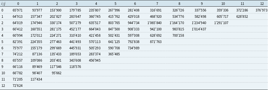
Example 1: Cumulative payments $(C_{i,\,j})$
.
$(C_{i,\,j})$
.
The true model parameters.

Example 1: Parameter estimates.
Example 1: Ultimate estimates and reserves at time I.

Example 1: The ultimate prediction error for aggregated accident years (as a percentage of the reserves).

Example 2: Cumulative payments $(C_{i,\,j})$
.
$(C_{i,\,j})$
.
Example 2: The ultimate prediction error for aggregated accident years (as a percentage of the reserves).

Expected squared deviation between $\textrm{estimator}^{1/2}$
and
$\textrm{estimator}^{1/2}$
and $\textrm{true value}^{1/2}$
, given
$\textrm{true value}^{1/2}$
, given $\mathcal{B}_0$
.
$\mathcal{B}_0$
.
Example 1 extended: Cumulative payments $(C_{i,\,j})$
.
$(C_{i,\,j})$
.

However, since the quantity (46) might not be the most appropriate and the three above-mentioned assumptions might not be consistent, from a theoretical point of view the assessment of the “goodness” of the three estimators might still be a subject for future research.
Example 2 extended: Cumulative payments $(C_{i,\,j})$
.
$(C_{i,\,j})$
.

Example 1: The ultimate prediction error for aggregated accident years (as a percentage of the reserves) for different triangles sizes.

Example 2: The ultimate prediction error for aggregated accident years (as a percentage of the reserves) for different triangles sizes.

Expected squared deviation between $\textrm{estimator}^{1/2}$
and
$\textrm{estimator}^{1/2}$
and $\textrm{true value}^{1/2}$
, given
$\textrm{true value}^{1/2}$
, given $\mathcal{B}_0$
, for different triangles sizes.
$\mathcal{B}_0$
, for different triangles sizes.

Probabilities of a high deviation from the true value, given $\mathcal{B}_0$
, for different triangles sizes.
$\mathcal{B}_0$
, for different triangles sizes.

4. Numerical Examples
Let us first analyse a simulated example.
4.1 A simulated example
Consider the cumulative payments $(C_{i,\,j})$
showed in Table 1 which have been simulated (for a given set
$(C_{i,\,j})$
showed in Table 1 which have been simulated (for a given set $\mathcal{B}_0$
and independently for each accident year i) by using the true parameters
$\mathcal{B}_0$
and independently for each accident year i) by using the true parameters $(f_j)$
,
$(f_j)$
, $(\sigma_j^2)$
specified in Table 2 according to the time series model
$(\sigma_j^2)$
specified in Table 2 according to the time series model
 \begin{align} C_{i,\,j+1}=f_j C_{i,\,j} + \sigma_j \sqrt{C_{i,\,j}} \varepsilon_{i,j+1},\end{align}
with $(\varepsilon_{i,j+1})$
i.i.d., uniformly distributed on
$(\varepsilon_{i,j+1})$
i.i.d., uniformly distributed on $[-\sqrt{3},\sqrt{3}]$
. Consequently, having additionally ensured positiveness of the data (see Model Assumptions 3.9 (time series model) and the related Remarks 3.10 in Merz & Wüthrich, Reference Merz and Wüthrich2008), these cumulative payments fulfil Model Assumptions 1.
$[-\sqrt{3},\sqrt{3}]$
. Consequently, having additionally ensured positiveness of the data (see Model Assumptions 3.9 (time series model) and the related Remarks 3.10 in Merz & Wüthrich, Reference Merz and Wüthrich2008), these cumulative payments fulfil Model Assumptions 1.
The set $\mathcal{B}_0$
by class of business.
$\mathcal{B}_0$
by class of business.

Performance study by class of business: The true model parameters and distribution assumptions.

Expected squared deviation between $\textrm{estimator}^{1/2}$
and
$\textrm{estimator}^{1/2}$
and $\textrm{true value}^{1/2}$
, given
$\textrm{true value}^{1/2}$
, given $\mathcal{B}_0$
, by class of business.
$\mathcal{B}_0$
, by class of business.

Also recall that when the true parameters are known, the true value $\textrm{PV}_{\textrm{tot}}+\textrm{EE}_{\textrm{tot}}$
for the ultimate prediction uncertainty can be computed analytically through formulas (16) and (18).
$\textrm{PV}_{\textrm{tot}}+\textrm{EE}_{\textrm{tot}}$
for the ultimate prediction uncertainty can be computed analytically through formulas (16) and (18).
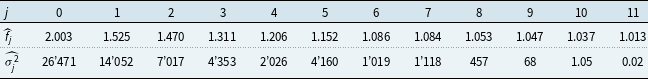
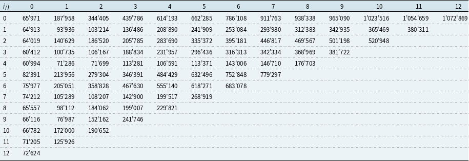
These data yield the parameter estimates related to Mack’s model, as indicated in Table 3, as well as the ultimate estimates $(\widehat{C}_{i,J})$
and reserves
$(\widehat{C}_{i,J})$
and reserves $(\widehat{C}_{i,J}-C_{i,\,I-i})$
at time I, as indicated in Table 4. Moreover, using estimators (39), (42), and (35), we can obtain the prediction uncertainties, as indicated in Table 5.
$(\widehat{C}_{i,J}-C_{i,\,I-i})$
at time I, as indicated in Table 4. Moreover, using estimators (39), (42), and (35), we can obtain the prediction uncertainties, as indicated in Table 5.
Given $\mathcal{D}_I$
, the empirical true value
$\mathcal{D}_I$
, the empirical true value $\textrm{PV}_{\textrm{tot}}+\textrm{EE}_{\textrm{tot}}$
is calculated by simulating the future claims payments (30’000 simulations using the true parameters
$\textrm{PV}_{\textrm{tot}}+\textrm{EE}_{\textrm{tot}}$
is calculated by simulating the future claims payments (30’000 simulations using the true parameters $(f_j)$
,
$(f_j)$
, $(\sigma_j^2)$
) and computing the average of the squared differences between simulated ultimate value and the ultimate estimate at time I given by
$(\sigma_j^2)$
) and computing the average of the squared differences between simulated ultimate value and the ultimate estimate at time I given by $\sum_{i=0}^I \widehat{C}_{i,J}$
. As expected, this numerical simulation yields a result that is well aligned with the true value.
$\sum_{i=0}^I \widehat{C}_{i,J}$
. As expected, this numerical simulation yields a result that is well aligned with the true value.
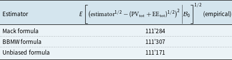
Table 5 indicates that the three formulas (Mack, BBMW and Unbiased) to quantify the ultimate prediction uncertainty yield similar results. However, the true value $\textrm{PV}_{\textrm{tot}}+\textrm{EE}_{\textrm{tot}}$
is considerably smaller than the estimated values, and, in this case, the Unbiased formula (35) achieves a result that is most similar to the true value.
$\textrm{PV}_{\textrm{tot}}+\textrm{EE}_{\textrm{tot}}$
is considerably smaller than the estimated values, and, in this case, the Unbiased formula (35) achieves a result that is most similar to the true value.
However, such a scenario does not usually occur. In fact, if another simulated triangle (see Table 6) based on the same true parameters and same set $\mathcal{B}_0$
is considered, the results presented in Table 7 are achieved. It can be noted that in this case, the BBMW formula yields the result closest to the true ultimate uncertainty.
$\mathcal{B}_0$
is considered, the results presented in Table 7 are achieved. It can be noted that in this case, the BBMW formula yields the result closest to the true ultimate uncertainty.
Finally, Table 8 presents the results of the performance simulation study (herein 50’000 triangles based on the same true parameters and same set $\mathcal{B}_0$
are considered) related to the expected squared deviation between estimator and true value, given
$\mathcal{B}_0$
are considered) related to the expected squared deviation between estimator and true value, given $\mathcal{B}_0$
. Here, it can be empirically observed that the Unbiased formula (35) slightly outperforms the other formulas.
$\mathcal{B}_0$
. Here, it can be empirically observed that the Unbiased formula (35) slightly outperforms the other formulas.
Increasing the number of available accident years related to the above considered examples, we get the data shown in Tables 9 and 10. Computing the prediction uncertainties at different points in time (i.e. for different triangles sizes), we get the results displayed in Tables 11 and 12.
From Tables 11 and 12, we can observe that, at each evaluation point in time, the three formulas do produce very close results. Moreover with increasing data availability, the possible gaps between estimators and true values reduce, since the estimators for the model parameters tend to get closer to the true parameters values.
In particular, as we can see from Table 13, at each evaluation point in time the Unbiased formula is performing slightly better than Mack and BBMW formulas. Moreover, the expected squared deviation between estimator and true value, given $\mathcal{B}_0$
, does decrease with increasing triangle size.
$\mathcal{B}_0$
, does decrease with increasing triangle size.
Remark 9. We highlight that all the considered triangles in this simulation study do fulfil the regularity condition (25). Also, we would like to further underline that deviations from the true value are ordinary and simply due to the random variable nature of estimators. Nevertheless, the large deviations we observed in our simulation study, as well as their high frequency (see Table 14), is noteworthy. Moreover, it is important to underline the key role played by the largeness of the data availability given by $I-J$
. Indeed, a large data availability helps to reduce the probability that estimator (35) does significantly differ from the true value. In other words,
$I-J$
. Indeed, a large data availability helps to reduce the probability that estimator (35) does significantly differ from the true value. In other words, $I-J$
should be sufficiently large (in fact larger than usually considered in the examples presented in actuarial literature or usually available in actuarial practice) in order to get an estimator which is well close distributed around the true value. A large data availability also helps to reduce the variance of the estimated sigma parameters which generally tends to be very high.
$I-J$
should be sufficiently large (in fact larger than usually considered in the examples presented in actuarial literature or usually available in actuarial practice) in order to get an estimator which is well close distributed around the true value. A large data availability also helps to reduce the variance of the estimated sigma parameters which generally tends to be very high.
4.2 Performance simulation study for different model parameter choices
Similarly as in the previous section, we simulate triangles according the time series model (49) with $(\varepsilon_{i,j+1})$
independent and shifted Gamma distributed with some given shape parameter
$(\varepsilon_{i,j+1})$
independent and shifted Gamma distributed with some given shape parameter $\alpha$
, with variance equal to 1 and expected value equal to 0. Then we run the performance analysis for different model parameter choices
$\alpha$
, with variance equal to 1 and expected value equal to 0. Then we run the performance analysis for different model parameter choices $(f_j)$
and
$(f_j)$
and $(\sigma^2_j)$
, which have been inspired by some real data triangles in actuarial practice. The studied data
$(\sigma^2_j)$
, which have been inspired by some real data triangles in actuarial practice. The studied data $\mathcal{B}_0$
are shown in Table 15, and the chosen model parameters for the different classes of business are shown in Table 16.
$\mathcal{B}_0$
are shown in Table 15, and the chosen model parameters for the different classes of business are shown in Table 16.
The results of the performance analysis (40’000 triangles considered for each model parameter choice) related to the expected squared deviation between estimator and true value, given $\mathcal{B}_0,$
are presented in Table 17. Again, it can be empirically observed that the Unbiased formula (35) slightly outperforms the other formulas.
$\mathcal{B}_0,$
are presented in Table 17. Again, it can be empirically observed that the Unbiased formula (35) slightly outperforms the other formulas.
4.3 Two real data examples
In this section, we analyse two real data examples. Note that in this case, there is also a model risk involved since we do not know, whether the data do exactly fulfil Model Assumptions 1 or not. Therefore, adding a loading on the three formulas is generally appropriate. This might also be the main reason why, based on various empirical studies on real claims data, there seems to hold a conjecture suggesting that the classical Mack estimator may be rather on the optimistic side.
4.3.1 The Merz-Wüthrich triangle
We consider the Private Liability triangle presented in Merz & Wüthrich (Reference Merz and Wüthrich2014) (see Table 18) and first observe that the regularity condition (25) is fulfilled.
The Merz-Wüthrich triangle: Cumulative payments $(C_{i,\,j})$
, estimated and guessed parameters.
$(C_{i,\,j})$
, estimated and guessed parameters.

Evaluating the three estimators for the ultimate prediction uncertainty, we get the results displayed in Table 19 and remark that the formulas lead to very close outcomes.
The Merz-Wüthrich triangle: The ultimate prediction error for aggregated accident years (as a percentage of the reserves).

The Taylor-Ashe triangle: Cumulative payments $(C_{i,\,j})$
, estimated and guessed parameters.
$(C_{i,\,j})$
, estimated and guessed parameters.

Since we do not know the true model parameters $(f_j)$
and
$(f_j)$
and $(\sigma^2_j)$
we cannot compute the true value
$(\sigma^2_j)$
we cannot compute the true value $\textrm{PV}_{\textrm{tot}}+\textrm{EE}_{\textrm{tot}}$
. However, based on the estimated parameters at time 16 we can make some rational guesses for the true model parameters and then compute the true value for the ultimate prediction uncertainty. By doing this, we observe that
$\textrm{PV}_{\textrm{tot}}+\textrm{EE}_{\textrm{tot}}$
. However, based on the estimated parameters at time 16 we can make some rational guesses for the true model parameters and then compute the true value for the ultimate prediction uncertainty. By doing this, we observe that $\textrm{PV}_{\textrm{tot}}+\textrm{EE}_{\textrm{tot}}$
could materially deviate from the estimated values. This is remarkable, because it means that if the cumulative payments will effectively evolve according to Model Assumptions 1 with model parameters as given by our guesses, then the true prediction uncertainty would materially deviate from the three available formulas. Moreover note that, when believing in the above mentioned empirical conjecture, we might conclude that our first two guesses are more realistic, because for these choices the true value
$\textrm{PV}_{\textrm{tot}}+\textrm{EE}_{\textrm{tot}}$
could materially deviate from the estimated values. This is remarkable, because it means that if the cumulative payments will effectively evolve according to Model Assumptions 1 with model parameters as given by our guesses, then the true prediction uncertainty would materially deviate from the three available formulas. Moreover note that, when believing in the above mentioned empirical conjecture, we might conclude that our first two guesses are more realistic, because for these choices the true value $\textrm{PV}_{\textrm{tot}}+\textrm{EE}_{\textrm{tot}}$
is bigger than the three estimated values, meaning that the real uncertainty is higher than indicated by the classical Mack formula. Also note that the difficulty in making a rational guess is highly driven by the sigma’s parameters, since the variances of
$\textrm{PV}_{\textrm{tot}}+\textrm{EE}_{\textrm{tot}}$
is bigger than the three estimated values, meaning that the real uncertainty is higher than indicated by the classical Mack formula. Also note that the difficulty in making a rational guess is highly driven by the sigma’s parameters, since the variances of $(\widehat{\sigma^2_j})$
are very high for the considered triangle size. In that respect, we remark that when having more accident years data at our disposal, the guessing procedure would likely be facilitated and the related true values will tend to be closer to the three formulas, as also indicated by the simulated example in section 4.1 (see Table 13).
$(\widehat{\sigma^2_j})$
are very high for the considered triangle size. In that respect, we remark that when having more accident years data at our disposal, the guessing procedure would likely be facilitated and the related true values will tend to be closer to the three formulas, as also indicated by the simulated example in section 4.1 (see Table 13).
4.3.2 The Taylor-Ashe triangle
We consider the triangle presented in Taylor & Ashe (Reference Taylor and Ashe1983) (see Table 20) and first observe that the regularity condition (25) is fulfilled.
Evaluating the three estimators for the ultimate prediction uncertainty, we get the results displayed in Table 21 and again remark that the formulas lead to very close outcomes.
The Taylor-Ashe triangle: The ultimate prediction error for aggregated accident years (as a percentage of the reserves).

Similarly to the previous example, we observe that the true value $\textrm{PV}_{\textrm{tot}}+\textrm{EE}_{\textrm{tot}}$
computed based on some rational guesses for the true model parameters could materially deviate from the three formulas. Moreover, the fact that the true value can be bigger than the estimated values for several model parameter guesses might also be a driver for the empirical conjecture suggesting that the classical Mack estimator may be on the optimistic side.
$\textrm{PV}_{\textrm{tot}}+\textrm{EE}_{\textrm{tot}}$
computed based on some rational guesses for the true model parameters could materially deviate from the three formulas. Moreover, the fact that the true value can be bigger than the estimated values for several model parameter guesses might also be a driver for the empirical conjecture suggesting that the classical Mack estimator may be on the optimistic side.
5. Conclusion
Within the chain-ladder model of Mack and under some additional technical assumptions, we derived a new estimator for the ultimate prediction uncertainty that is unbiased (conditionally given the first triangle column). Unluckily, from a theoretical point of view, the unbiased estimator does also show some peculiar behaviours, in particular with respect to its possible negativity. However, from a practice point of view, these behaviours do not create difficulties when considering typical insurance data. Also, the required additional technical assumptions can be reasonably assumed to hold true, since they are consistent with data typically encountered in actuarial practice, and should not be confused with the strong (and possibly inconsistent) assumption of positivity along all the (finite) trajectories of the claims payments process.
Furthermore, we underline that the three considered formulas (Mack, BBMW and Unbiased) produce extremely similar results, and the differences may not be significant for applications in actuarial practice.
Therefore, using the straightforward explained Unbiased formula (which deliver the smallest result) does not lead to any relevant misestimation of reserve risk compared to the Mack and BBMW formulas, also in case the true value occurs to be bigger than its estimators.
Indeed, we demonstrated that all three estimators can, with non-negligible probability, materially fail to quantify the true uncertainty, especially when considering small or average-sized triangles often available in practice.
Acknowledgements
I would like to thank Prof. Dr. Mario Wüthrich for fruitful discussions on earlier versions of this manuscript which made me aware of the unbiasedness property of the new proposed estimator. Also, I would like to thank the Editor and several anonymous reviewers for their helpful comments and inputs which permitted to improve the quality of the paper.


 Open access