2.1. The ice dynamics model

The thermomechanically coupled scheme is designed and implemented as one integral component of a scalable and extensible geofluid modelling system, SEGMENT (Reference RenRen and others, 2009). By synthetically solving the three-dimensional conservation equations for mass, momentum and energy under multiple rheological relationships, SEGMENT provides prognostic fields of the driving and resistive forces, and describes the flow fields and the dynamic evolution of thickness profiles of the medium (ice in this case). The inner ice domain follows the Reference GlenGlen (1955) ice rheology. A granular layer is allowed between ice and unfractured bedrock. The granular viscosity parameterization is based on Reference Jop, Forterre and PouliquenJop and others (2006). Many ice models use only ice-over-bedrock configurations. In contrast, SEGMENT-Ice has an ice–granular-material–bedrock configuration for regions with granular material present, mostly for regions with significant basal melting. Reference Ren, Fu, Leslie, Karoly, Chen and WilsonRen and others (2011a) provide the formulation of the granular law; justification of the granular layer; the omission of isostatic rebound; discussion of consistent choices of ice constitutive law and Weertman basal sliding; new approaches in parameterizing surface melting and runoff; the crevasse enhancement of basal sliding; and sea-water–ice interaction at the calving front.

Parameterization of viscosity is critical for ice creep. SEGMENT-ice has two improvements over Glen’s ice rheological law (Reference HookeHooke, 1981; Reference Van der VeenVan der Veen, 1999), factoring in the flow-induced anisotropy and granular basal conditions. The flow enhancement by re-fabricating (Reference Wang and WarnerWang and Warner, 1999) is implemented, so older ice, farther from the Summit, is easier to deform. SEGMENT-ice also allows a lubricating layer of basal sediments between the ice and bedrock which enhances ice flow and forms a positive feedback for mass loss in a warming climate (Reference MacAyealMacAyeal, 1992; Reference Alley, Lawson, Larson, Evenson and BakerAlley and others, 2003; Reference Ren, Fu, Karoly, Leslie, Chen and WilsonRen and others, 2010; Fig. 2, further below). Because the ocean temperature is higher than that around Antarctica, there are no ice shelves around Greenland. However, there are several water-terminating fast glaciers around the periphery of GrIS, such as Jakobshavn (J), Kangerdlugssuaq (K), Helheim (H) and Petermann (P) glaciers. In SEGMENT-ice, ocean–ice interactions are parameterized so that the depressing of the freezing point by soluble substances, the salinity dependence of ocean water thermal properties and the ocean-current-dependent sensible heat fluxes are all included.

As the climate warms, increased air temperature through turbulent sensible heat-flux exchange increases surface melting and runoff. Similarly, changes in precipitation affect the upper boundary input to the ice-sheet system. For the period of interest here, major ice temperature fluctuations are near the upper surface of the GrIS. The strain rate, however, can be large near the bottom, so SEGMENT-ice has a 31-vertical-level, stretched grid to better differentiate the bottom and near surface. The uppermost layer is 0.45 m thick near the GrIS Summit (e.g. gridlines in inset of Fig. 1), fine enough to simulate the upper surface energy state on a monthly timescale. Because of its location, the GrIS is an important contributor to eustatic SLR, ocean salinity and North Atlantic thermohaline circulation (Reference AlleyAlley, 2000). In SEGMENT-ice, the total mass loss comprises surface mass balance and the dynamic mass balance due to ice flow divergence.

Fig. 1. Land-cover mask for the Greenland ice sheet. The locations of Jakobshavn (J.), Kangerdlugssuaq (K.), Petermann (P.) and Helheim (H.) glaciers, the northeast Greenland ice stream (NE.) and the Summit (SMT) are labeled. Hatched areas are regions with ice loads but with bottom elevations lower than the present sea level. Red box delimits the 1 km simulation of Jakobshavn Isbræ in Figure 6. Inset is a zoomed Petermann Glacier (south is to the left), a vertical cross-section along the vertical red line.

In ice flow, inertial and viscous terms counteract pressure gradient forces. The full Navier–Stokes equations are used in the momentum equations of SEGMENT-ice. Because of comparably large aspect ratios, ice streams and surrounding transition zones are the areas where a full Stokes model is most needed (Reference Zwinger, Greve, Gagliardini, Shiraiwa and LylyZwinger and others, 2007). Finally, there are two important improvements in the SEGMENT-ice numerics. Recently, the Robert–Asselin–Williams (RAW; Reference WilliamsWilliams, 2011) filter has been adopted, in place of the more commonly used Asselin time filter. This treatment has improved both spin-up and the conservation energetics of the physical processes. A second improvement is in the optimization procedure of the data assimilation code. A quasi-Newton minimization scheme is now used instead of the conjugate-gradient scheme which is less robust and less efficient for real, noisy data.

Relevant to the first positive feedback mechanism identified in this study, SEGMENT-ice has a unique ice-shelf component that considers the heat transfer between ice and the surrounding sea water as an aqueous solution of five major electrolytes (Cl⁻, Na⁺, Mg²⁺, SO₄ ²⁻and Ca²⁺) and the subsequent ice formation and melting at the interface. Sea water is an aqueous solution of many electrolytes. The physical properties of this solution that are relevant for heat transfer are thermal conductivity, λ, density, ρ, heat capacity under constant pressure, c_p , and kinematic viscosity, v. The heat transfer from liquid (the sea water) to solid (the ice in contact with sea water), Q _h, is also related to the liquid flow property, measured as Prandtl number and Grashof number, to measure whether the natural or forced heat conductance dominates. Under typical conditions in the polar seas surrounding Greenland, a turbulent boundary layer is a more accurate approximation. The ocean currents around Greenland are complicated. The East and West Greenland Currents transport cold and fresher water that meets the subtropical warm and saltier waters from the Irminger Current, a topographically steered branch of the North Atlantic Current. Fresh water occurs in the vicinity of the glacier environment in the upper 100 m, but strong mixing and density-driven circulations are plentiful at greater depths. Recent observations confirm that there are vigorous circulations even under a glacier terminus (e.g. Reference Rignot, Koppes and VelicognaRignot and others, 2010; Reference StraneoStraneo and others, 2010). Thus, we propose that

(1)

where ρ is sea-water density, c_p is specific heat of sea water, u is sea-current speed, T_l is sea-water temperature, T_s is ice surface temperature and C _H is a stability-dependent heat transfer coefficient ((3 × 10⁻⁶)−10⁻⁵). Note that ρ, c_p and C _H are all functions of salinity S (the molar fraction of electrolytes over water).

There is a problem concerning freezing-point depression by electrolytes in solvent. When the solution reaches solid (ice)–liquid (sea-water) equilibrium, the chemical potential of the solvent is equal between the liquid and the solid phase (Raoult’s law). The molar Gibbs free energy for liquid phase is defined as

(2)

where T is temperature, P is pressure, R ^* is the ideal gas constant and a is the activity of the solvent. The chemical potential for the solid state is similarly defined as

(3)

According to the Gibbs–Helmholtz equation,

(4)

where h ₀ ^″ is the enthalpy of pure water and h ₀ ^′ is the enthalpy of pure ice. Thus Δh(T) = (h ₀ ^″ – h ₀ ^′) is the enthalpy change of fusion and can be parameterized linearly around the triple point along an isotherm:

Here is heat capacity and I″-′ = Δh(T_f), where ″ denotes liquid states and ′ denotes solid states, is usually termed latent heat of fusion. Integrating Equation (4) along an isotherm from the triple point of pure water, T_f, to an arbitrary temperature T, gives

(5)

For a given value of a (molar concentration of solutes), Equation (5) can be solved numerically to obtain an equilibrium temperature, T. In SEGMENT-ice, Equation (5) is used in determining phase change of ice in contact with sea water. This parameterization is relevant for water-terminated glaciers (e.g. Helheim Glacier) and ice streams.

2.2. Climate model forcing

This study investigates both atmospheric and oceanic driving of GrIS melting, especially for ocean-terminating fast outlet glaciers. The key controls on melting, such as volume and properties of subtropical water intrusion, the alongshore wind patterns and the associated changes in weather patterns, likely are intertwined. Therefore, CGCMs provide the predicted atmospheric and oceanic parameters to drive the SEGMENT-ice model.

Refining the horizontal model resolution improves the regional simulations of precipitation (Reference GenthonGenthon 1994; Reference Ohmura, Wild and BengtssonOhmura and others, 1996). Thus, two CGCMs with relatively fine horizontal resolutions, the NCAR CCSM3 (Reference CollinsCollins and others, 2006; ∼1.4°) and MIROC3.2 (Reference Hasumi and EmoriHasumi and Emori, 2004; ∼1.125°), were chosen. These CGCMs provide all input variables needed by SEGMENT-ice, i.e. monthly-mean near-surface air temperature, precipitation rate, surface (skin) temperature, surface pressure, 2 m wind speed and all six components of radiation for determining the surface energy balance. For ice melting, SEGMENT-ice (Reference Ren, Fu, Leslie, Chen, Wilson and KarolyRen and others, 2011b) uses an energy-balance scheme instead of the positive degree-day (PDD) schemes which are popular in ice models applied to paleoclimate studies. Estimates of the warming effects on ice-sheet melting are based on the IPCC Special Report on Emissions Scenarios (SRES) A1 B scenario, which assumes a balanced energy source in a future world of rapid economic growth. This scenario is chosen primarily because it reflects the most recent trends in the driving forces of emissions.

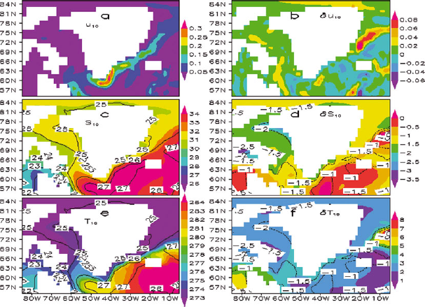
In addition to atmospheric parameters, to investigate the ice–ocean interactions at Jakobshavn, Kangerdlugssuaq, Helheim and Petermann glaciers, the ocean flow speed, , potential temperature, T, salinity, S, and density, ρ, are also needed. Density is not an independent property since it is a function of temperature, salinity and pressure. That is, it is a function of salinity and potential temperature. For the outlet glaciers north of 70° N, the CCSM and MIROC-hires ocean model outputs at 0, 10, 20, 30, 50, 75 and 100 m depths are interpolated to SEGMENT-ice grids. The top 100 m of sea water has similar spatial patterns of the physical properties and similar temporal variations. Therefore plots are shown only of the near-surface (10 m depth) ocean parameters (Fig. 2). For Helheim Glacier, which resides in the Sermilik Fjord, the 1 km resolution ice-thickness data obtained from the SeaRISE project (http://websrv.cs.umt.edu/isis/index.php/Main_Page) indicate that the terminus depth is ∼700 m, close to the estimation of Reference ThomasThomas and others (2000). Oceanic parameters up to 1000 m are used for this glacier. At present, none of the climate models has a coupled land-ice component, so the limited salinity changes (Fig. 2b and e) are due primarily to precipitation changes and changes in river routing and, to a lesser degree, circulation adjustments. The model (Fig. 2f) shows significant warming of ocean water around the GrIS from the surface to 100 m.

Fig. 2. Oceanic forcings shown at 10 m depth. (a) Flow speed (m s⁻¹), (c) salinity (psu) and (e) potential temperature (K), with changes over the 21st century shown respectively in (b), (d) and (f). Contours in (c) and (e) are potential density (kg m⁻³, difference from 1000 kg m⁻³) and are the same in both panels. Contours in (d) and (f) are changes in potential density.

3.1. Impacts of ocean water interactions

Freezing-point temperatures at the four selected fast glaciers are respectively −1.6, −1.7, −1.65 and −1.66°C at Jakobshavn, Helheim and Petermann glaciers and the northeast Greenland ice stream. Figure 3 shows the projected additional ice retreat due to interactions with sea water (the combined results of water warming and freshening). By 2100, the calculated net retreats from ocean contribution are 327, 87, 57, 728 and 682 m for the northeast Greenland ice stream and Petermann, Kangerdlugssuaq, Helheim and Jakobshavn glaciers respectively. To the southeast of the GrIS (e.g. Kangerdlugssuaq and Helheim glaciers), the ocean salinity is already low (28 psu at surface level) and the contributions from water freshening are small (<5%). At Jakobshavn Isbræ, it can be as large as 15%. For the same temperature differences between ice and liquid/gas, water is five times more efficient in melting ice than air, due to its higher bulk heat-transfer coefficient. Although for ocean water the heat transfer coefficient, C _H, is three orders of magnitude smaller than for air, its density is three orders of magnitude larger than for air, and its specific heat is four times larger than for air. Reference HuHu and others (2010) prove that the surface water salinity can fluctuate about 2 psu on glacial timescales. If current climate change is more significant than historical natural climate changes, a sensitivity experiment is performed assuming a 5 psu fluctuation of the upper 1000 m of sea water. If other factors are unchanged, the contribution from the freshening of sea water is <3% of the sensible heat transfer between ice and sea water.

Fig. 3. Terminus retreat for five fast glaciers at the margin of the GrIS: Helheim (H.), Jakobshavn (J.) and Kangerdlugssuaq (K.) glaciers, the northeast Greenland ice stream (NE.) and Petermann Glacier (P.). The retreat is perpendicular to the interface. Dotted lines indicate that the glaciers are likely to be totally land-terminated by that time, and the direct ocean effects will suddenly disappear.

Note that the additional melting due to freshening is small compared with that of ocean water warming. The ocean water influence on the GrIS outlet glaciers is limited because the interfaces are only a small fraction of the entire grounding line and because some of the water-terminating glaciers will be land-terminating during the 21st century (e.g. Kangerdlugssuaq and Helheim glaciers in Fig. 3). From Figure 1, the bedrock elevations for the outlet glaciers are below sea level. There are always ocean/ice interfaces before the grounding line retreats to locations above sea level.

At the base of water-terminating glaciers (Fig. 4), the interface is usually slanted so the water cavity is wedge-like. The angle, θ, can be small (typically several degrees) to form ice shelves, or moderate to form landlocked ice. For numerical modelling, we set the stress tangential to the water/ice interface to be zero. The normal stress is the hydrostatic stress of the water at that depth. Inside the ice, the imbalance of stresses is compensated by viscous creep. Thermodynamically, turbulent sensible heat fluxes and phase changes are allowed at the interface. As the ice always melts from below, the tongue is lowered to meet the hydrostatic balance requirement. In SEGMENT-ice, the yield strength of the solid ice is prescribed so that when the yield strength is exceeded, crevasses occur. As ice is brittle, even at temperatures close to the melting point, a lowering of the ice tongue is usually accompanied by cracking. The reverse is true when ice accumulates at the interface. The actual fluctuation of the grounding line location is a dynamic balance between melting/condensing and flow divergence. To convert retreating into grounding-line retreat, the angle effects should be factored in, as they affect the melting fraction contribution. For Helheim Glacier, the grounding line retreat reaches 80 km by the end of this century from the ocean contribution alone, and may render this glacier totally land-terminated by that time.

Fig. 4. Schematic of a water-terminating glacier. The water/ice interface cavity is usually wedge-shaped with angle θ. The model calculates the ice retreat normal to the interface. The grounding line retreat should be estimated with a multiplicative factor 1/tan θ which can be up to O(10²) in magnitude. The portion that extends to sea (L _c) is limited by climate conditions, primarily by ice mass turnover rate and ocean temperature. Ice is brittle because its low melting-point diffusivity is ∼10⁻¹⁵ m² s⁻¹. The limiting length L for shelf break is a good indicator of grounding line retreat. θ increases as the climate warms. If the ice sheet is primarily land-based, the ocean’s effect diminishes as the grounding line retreats to ground above sea level (point N).

The GrIS meltwater routing into surrounding waters might have an effect on the AMOC analogous to the inter-basin freshwater transfer effects (Reference MolnarMolnar, 2008). For example, relatively fresh North Pacific water can enter the Arctic Ocean through the Bering Strait and go further into the North Atlantic through the clockwise Arctic Ocean surface current. Reference HuHu and others (2010) found that the opening and closing of the Bering Strait corresponds well with the eustatic sea-level oscillations on subglacial temporal scales (∼20 ka). This is not explicable by solar radiation and albedo positive feedback alone, as they both vary smoothly within the 116 ka last glacial period. This identified self-constraint mechanism is the strengthening and slackening of the AMOC. When the AMOC is strong (e.g. when the Bering Strait is completely shut down by a drop in sea level or is frozen when the sea water is relatively shallow) the northward heat transfer is strong and persists for many thousands of years. This will cause a drastic shrinkage of ice sheets and an associated global SLR. The opposite phase is a strong mixing of surface water from the Arctic Ocean and a weakened AMOC resulting in a colder environment that favours expansion of glaciers and ice sheets. At present, the runoff water from the GrIS melting may act in a similar way to weaken the AMOC, but to a much smaller extent when compared with Pacific–Atlantic water mixing. It is a checking mechanism for enhanced melting as climate warms (i.e. a negative feedback). However, the Reference HuHu and others (2010) results cannot be taken literally in the current human-induced climate-warming context. The current warming trend is not comparable with the natural oscillatory climate variability, as it has a human component with an upward trend. This implies a net total energy build-up within the climate system. Even when the AMOC weakens, atmospheric components may assume the poleward energy-transporting role.

3.2. Impacts of strain heating

The evolution of ice-sheet geometry configuration is governed by competition between the net accumulation rate, which is climate-governed, and the divergence/convergence of gravitationally induced ice velocity, which is flow-governed. Ice microphysical processes regulate the character of the ice flow, especially the dependence of viscosity on strain rate and temperature. For a given ice thickness, bedrock geometry and temperature profile within the ice, an equilibrium flow field is obtainable. To maintain exact balance, the flow-induced strain heating must be removed completely by reversible means. Additionally, flow caused by divergence/convergence must be exactly balanced by surface net accumulation/ablation. As a consequence, exact balance is never reached. In the following discussion of strain heating, it is assumed that a nearly balanced state exists so that the ice geometry does not vary significantly.

Strain heating can be expressed as (Reference GreveGreve, 2005), where v is ice viscosity and σ_eff is effective stress (Pa) expressed as , with tr being the trace function and σ being the deviatoric stress tensor. Assuming constant geometry and temperature field within the ice sheet, strain heating can be expressed as , where A is the temperature-dependent ice fluidity, related to the activation energies for ice deformation. At the same time, is a temporal constant. Thus, it is straightforward to show that, for two temperatures T₁ and T₂, the ratio of strain heating is A(T₁)/A(T₂). In the derivation, enhancement factors are omitted and only the parameterization of Reference PatersonPaterson (1994) is used.

Figure 5 shows the near upper surface (10 m depth) strain-heating changes estimated according to MIROC-hires estimated atmospheric parameters. For each line segment, the starting point corresponds to the 2000 situation and the end point corresponds to the 2100 situation. The absolute values for different fast glaciers are also quite different as they depend on ice geometry. Thus, it is less meaningful to make cross comparisons between different locations. For each glacier, strain-heating values are plotted against strain heating at −35°C. The A(T) curve is also plotted to provide a reference. Integrating the ice model with the SRES A1B scenario until 2100, we find that ice temperatures at Jakobshavn, Petermann, Kangerdlugssuaq and Helheim glaciers, Summit and Southern Dome increase by 1.8, 3.7, 2.8, 3, 2.42 and 2.6°C respectively over the 100 year period. As a result, for Petermann Glacier, the strain-heating rate, in the near surface at 10 m depth, will almost double by 2100. Strain-heating rates at Jakobshavn and Kangerdlugssuaq glaciers are already quite high, but will increase as the temperature increases (there is a ∼80% increase from 2000 to 2100). Increased strain heating will be significant over all the GrIS, so as long as the air temperature keeps increasing, the strain-heating rate also increases.

Fig. 5. Strain-heating rate relative to the rate at −35°C at six stations: Summit (SMT), Petermann Glacier (P.), Southern Dome (SD), Kangerdlugssuaq (K.), Helheim (H.) and Jakobshavn (J.) glaciers. The starting point corresponds to the value in 2000; the end point corresponds to the value in 2100. To differentiate clearly between locations, the Petermann Glacier data are indicated by a red dashed line, the Southern Dome data by a blue line, and the Helheim Glacier data by a green line.

The ‘grade-glacier’ theory (Reference Hallet, Hunter and BogenHallet and others, 1996 and references therein; Reference Alley, Lawson, Larson, Evenson and BakerAlley and others, 2003) generalizes silt production and transportation as an integrated component of ice erosion on the glacier bed. It shows that climate fluctuations, by modifying ice surface slope, can affect sediment transport and erosion patterns. This theory partially motivated the granular basal sliding treatment because the established warming climate may flatten the marginal area of the fast glaciers surrounding the GrIS and encourage the deposition of granular sediments. This is a positive feedback because granular basal sliding enhances ice divergence to downstream locations which are not in equilibrium even with current climate conditions, and hence the ice melts rapidly. The meltwater thus generated enhances granular material production. The detailed parameterization of granular material viscosity can be found in Reference Ren, Fu, Karoly, Leslie, Chen and WilsonRen and others (2010, Reference Ren, Fu, Leslie, Karoly, Chen and Wilson2011a,Reference Ren, Fu, Leslie, Chen, Wilson and Karolyb). This erosion positive feedback explains why the fast glaciers usually have bedrock elevations lower than the surrounding regions (ice lying in trenches) and usually are below sea level (e.g. H., J. and K. glaciers in Fig. 1). For example, the bedrock topography at Jakobshavn Isbræ may initially be a slight depression. With the positive feedback of ice viscosity enhancement (the larger the slope, the smaller the viscosity as time elapses), the ice speed increases and the ice flow forms a stream as it becomes narrower and more concentrated than sheet flow. As the ice flows faster, the erosion rate increases and more granular material is produced at the bottom. Granular material has a much smaller viscosity than solid ice and the flow is greatly enhanced and the generated granular material is effectively transported downstream. As these positive feedbacks continue, a deeper trench of the order of hundreds of metres is produced and the trench extends upstream. If the ice were suddenly removed, Greenland would become three major islands separated by shallow ocean waters.

3.3. Impacts of granular basal sliding

Granular material can be widely available under an ice sheet because, during the glacier’s history, around the grounding line repeated phase changes between ice and water are highly effective mechanisms for producing granular material. The process is several orders of magnitude faster than uniform weathering by runoff water. To study ice-sheet flow, granular material under solid ice is less important than that located under a melting base. To first order, the subglacial geochemical environment consists of finely crushed rocks bathed in ice melt, analogous to the flow-through reactors used to measure mineral weathering rates (Reference Anderson and KnightAnderson, 2006). For SEGMENT-ice, the input parameters are granular layer thickness and effective grain size. Obtaining the granular layer thickness is difficult because both the production rates and the subglacial flow washout rate are required (Reference Cutler and KnightCutler, 2006). With sufficient surface ice-flow observations and known ice temperature distributions, the granular parameters can be objectively retrieved by the data assimilation routine of SEGMENT-ice. The retrieved granular material thickness and effective size are used only as initial conditions. Their subsequent evolution is parameterized according to Reference Anderson and KnightAnderson (2006), using an erosion scheme with temperature- and geology-dependent multiplicative factors.

3.4. Case study: Jakobshavn Isbræ

Jakobshavn Isbræ lies at the intersection of the three positive feedbacks described in the preceding subsections. From Figure 1, if the ice is completely removed, Greenland becomes three islands separated by shallow ocean waters. Geologically, Jakobshavn Isbræ is located in the valley between the largest middle island (containing the Summit, SMT in Fig. 1) and the southern island (containing the Southern Dome, SD). The largest surface slope angle is ∼9° at 1 km resolution, one of the steepest surface slopes on the GrIS. At the interface with ocean water, there is ∼550 m deep ice below sea level and the width of the mouth is ∼6 km (hence the vertical cross section is ∼3 km² at the ocean/ice interface). Because of its southern location (69° N), the ice temperature is relatively high, with a surface annual mean temperature of about −10°C.

A model simulation of the entire GrIS was made at 1 km horizontal resolution, but only the flow changes between 2000 and 2100 for the Jakobshavn Isbræ vicinity are shown here (Fig. 6). Meteorological forcing parameters are from CCSM3 under the SRES A1B scenario emissions assumption. Figure 6a is a model-simulated present-day surface level ice-flow velocity, and Figure 6b shows the flow vertical profile changes over the 2000–2100 period, near the bottleneck leading to the present mouth (‘+’ in Fig. 6a). The flow is concentrated, and maximum velocity cores indicate primarily westward speeds of >8000 m a⁻¹. In addition to the positive feedback of granular basal sliding, the concentrated ice flow arises from the steep bedrock geometry and the reduction in ice viscosity. Because of the large magnitude of flow divergence/convergence, large fluctuations in ice geometry adjustment are expected, on decadal timescales. However, ocean discharge will always be significant. We show a limited simulation domain (49.97W, 68.883N at the left lower corner to 48.42W, 69.44N at the right upper corner). Viewed from the entire GrIS, this ice stream drains a large sector of the ice sheet (∼7% of the total area). Integration along the ocean/ice interface of the cross product of ice velocity and unit normal of the interface indicates that the present ice speeds supply ∼23 km³ a⁻¹ to the ocean.

Fig. 6. SEGMENT-ice simulation of the ice flow field at Jakobshavn Isbræ (red box in Fig. 1). (a) Year 2000 surface (u, v) velocity. (b) The u-velocity profile at a point near the mouth (ice/ocean interface, ‘+’ in (a)) for 2000 and a projected 2100 profile (dashed line). Ice flow is faster in 2100 because the ice temperature is higher; the back force from ocean hydrostatic pressure is lower because the tongue thins as ocean melting increases, and there is increased granular basal sliding speed. Including ice-thickness changes, the discharge rate at the mouth of Jakobshavn Isbræ has increased by ∼1.2 km³ a⁻¹(∼5% of year 2000 value) by 2100. 1 km resolution ice geometry data are used in the model simulation. Meteorological fields for the projection are from CCSM3 under the SRES A1B scenario.

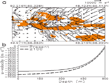
There is an expected increase in flow speeds in the 21st century (Fig. 6b), as a result of interactions between ocean warming, air warming and increased granular basal sliding. Ice surface elevation over this small area is insignificant because of a dynamic equilibrium between increased ice discharge and the increased ice flow at the upper stream source region. Compared with the year 2000 level, annual ice discharge into the ocean could increase by ∼1.4 km³ a⁻¹ (∼5% of the present annual rate) by 2100. The grounding line is steadily retreating. By 2050 the ice/ocean interface may retreat to the ‘+’ sign location, and by 2100 to the location of the double dashed blue line. Because of the complicated bedrock topography, the ice/ocean interface may be separated into two segments by 2100 (Fig. 6a). The southern branch has deeper (1000 m) ice layers lying below sea level than the wider, northern branch, which has <100 m ice lying below sea level. Also the ice speed is larger for the southern branch (∼8500 m a⁻¹)than the northern branch (700 m a⁻¹). Hence the ice/sea interaction is primarily through the southern branch. The southeast areas below sea level (right lower corner in Fig. 6a) cannot interact with the ocean water in the transient climate change period as they have no direct connection to the ocean.

Ice thickness near the mouth is ∼600 m. At the bottom, basal sliding contributes a sliding speed of ∼90 m a⁻¹ at present, increasing to ∼400 m a⁻¹ by 2100 (Fig. 6b). The ice velocity profile within the thin (∼1 m) granular layer is dilatant, but flow is shear-thinning above that layer. The 300 m a⁻¹ increase thus adds almost uniformly to the 600 m thick ice.