


Near-surface temperature is among the most important external forcings for ice-sheet models studies. It defines where and how much snow and ice is lost from an ice sheet through surface melt. In currently glaciated areas such as Greenland and Antarctica, an increasing number of near-surface temperature measurements are available from automatic weather stations (Steffen and others, 1996; Ahlstrøm and others, 2008; van As and others, 2014). Owing to the fact that ice sheets typically have smooth geometries and large horizontal dimensions, the overlying atmospheric conditions are characterized by smooth near-surface temperature fields, which are, to a great extent, modulated by ice-surface elevation. This enables a spatial interpolation between in situ measurements using an intrinsic linear relation between the surface elevation and near-surface temperature, which is commonly termed a slope lapse rate (here and in the following the slope lapse rate is defined to be positive, if the near-surface temperature decreases with elevation) (Ritz and others in Reference Ritz, Fabre and Letréguilly1997; Fausto and others in 2009).
A slope lapse rate indicates the rate of near-surface temperature decrease with elevation and generally differs from the free-air lapse rate or the rate of moist adiabatic cooling, which is normally within the range of 6–7°C km−1 (Marshall and others, Reference Marshall, Sharp, Burgess and Anslow2007; Fausto and others, Reference Fausto, Ahlstrøm, Van As, Bøggild and Johnsen2009; Gardner and others, Reference Gardner2009). Analyses of existing observational data in Greenland have shown that slope lapse rates vary significantly through the year, with lower lapse rates recorded over melting glaciers close to the ice-sheet margin (Hanna and others, Reference Hanna2005; Stone and others, Reference Stone, Lunt, Rutt and Hanna2010). In glacial modeling studies, slope lapse rates (especially over the melting period) play a critical role, and are often used as tunable parameters (e.g. Gardner and others, Reference Gardner2009). The modeling experiments of Stone and others (Reference Stone, Lunt, Rutt and Hanna2010) have demonstrated that an increase in the summer slope lapse rate by ~1.6°C km−1 leads to an increase of up to 50% in the modeled present-day volume of the Greenland ice sheet. The outcomes of stand-alone paleo ice-sheet simulations emphasize an even stronger influence of lapse rates on the modeled volumes of the former ice sheets, which depend strongly on how near-surface temperature forcing is modified during the inception, growth and decay of ice sheets. For example, Abe–Ouchi and others (Reference Abe–Ouchi, Segawa and Saito2007) tested the sensitivity of the former Northern Hemisphere ice sheets to changes in slope lapse rates by 1–2°C km−1 and revealed that such changes triggered differences of 50–250% in the modeled ice volume during the Last Glacial Maximum (LGM). It is therefore important to understand whether the present-day estimates of slope lapse rates from ice-covered regions are appropriate for modeling ice sheets under climate conditions that are different from modern.
Using observational data from four glaciers in the Canadian high Arctic and climate reanalyses, Gardner and others (Reference Gardner2009) suggested a negative relation between near-surface lapse rates and lower-troposphere temperatures. Here we seek to extend their analysis to glacial-interglacial timescales by comparing the slope lapse rates that would arise from the two extreme climate states of the last glacial cycle, namely the Holocene and the LGM. For this purpose, we use the outputs of paleoclimate modeling experiments to derive the LGM, early Holocene, and pre-industrial climate states and compare our model results with observation-based lapse rates. Our study focuses on the Greenland ice sheet, since it is an ideal target for such an analysis. Although the Greenland ice sheet was more extensive during the glacial period (in many places reaching the continental shelf break), changes in its geometry since the LGM can be considered minor compared with the regions that were entirely buried under continental-scale ice masses during the LGM and had undergone a complete deglaciation during Termination I (O'Brien and others, Reference O'Brien1995; Johnsen and others, Reference Johnsen1997; Rasmussen and others, Reference Rasmussen2006). Greenland can therefore serve as a reference region for a nearly one-to-one evaluation of the Holocene and LGM boundary layer conditions over ice-sheet surfaces.
1. METHODS
In this study, we analyze three near-surface temperature fields derived from the coupled general circulation model CCSM3 (Community Climate System Model, version 3.0, Collins and others, Reference Collins2006; Fig. 1). CCSM3 is composed of four separate model components that simultaneously simulate atmosphere, ocean, sea ice and land surface interacting through a central model coupler. For this particular study, the treatment of the atmospheric boundary layer processes in the climate model is of utmost importance. In CCSM3, the turbulence parameterization includes an explicit, non-local atmospheric boundary layer parameterization, while surface exchanges of heat, moisture and momentum are treated with bulk exchange formulations following Monin–Obukhov similarity theory (Collins and others, Reference Collins2004).
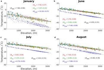
Modeled near-surface temperatures (vertical axes; °C) versus surface elevation (horizontal axes), (m), for the coldest month and the melting period derived from the pre-industrial (PI, red), early Holocene (EH, green) and Last Glacial Maximum (LGM, blue) climate simulations. Yellow diamonds and cyan triangles mark the measurements from the GC-Net (Steffen and others, Reference Steffen, Box and Abdalati1996) and PROMICE (Ahlstrøm and others, Reference Ahlstrøm2008; van As and others, Reference van As, Fausto and Steffen2014) stations, respectively. Gray and black lines denote the results of the weighted least-squares regression for the climate simulations and observations, respectively.

We performed simulations of the pre-industrial, early Holocene and LGM climate conditions with a relatively high atmosphere model resolution of T85, approximately corresponding to 1.4° and 26 levels in the vertical (Prange and others, Reference Prange, Steph, Liu, Keigwin, Schulz, Schulz and Paul2015). Our pre-industrial and LGM climate simulations follow the protocols established by the Paleoclimate Modelling Intercomparison Project Phase 2 (PMIP2, Braconnot and others, Reference Braconnot2007) and share identical setups with the CCSM3 runs presented as part of the PMIP2 (Otto-Bliesner and others, Reference Otto-Bliesner2006), but with a twofold increase in the horizontal resolution of the atmosphere and land components. Following this protocol, for the pre-industrial simulation we have applied the greenhouse gas concentrations, ozone and aerosol distributions appropriate for the time before industrialization (ca 1800). The LGM simulation utilizes the orbital parameters, greenhouse gas concentrations, sea-level lowering and the ice-sheet configurations of 21 000 years before present. For the early Holocene simulation, we used the orbital parameters and greenhouse gas concentrations for 8500 years before present (CO2 = 260 ppmv, CH4 = 660 ppbv, N2O = 260 ppbv). All other forcings were the same as in the pre-industrial simulation. For each simulation, the model has been run over a period of 1400 years to attain a quasi-equilibrium state. 100-year averages of the climate model outputs have been used to infer the monthly slope lapse rates for the LGM, early Holocene and pre-industrial periods (Fig. 2).
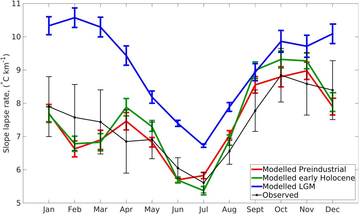
Evolution of slope lapse rates through the year as inferred from the LGM (blue), the early Holocene (green) and pre-industrial (red) climate simulations and observations (black). Vertical bars mark the corresponding standard errors.
A linear relation between near-surface temperatures and ice surface elevation in Greenland has been derived using a 1/σ 2-weighted least-squares regression applied to the mean monthly temperature fields across a range of ice elevations above 500 m (Fig. 1). Our choice of the lower elevation limit (500 m) is motivated by the fact that the resolution of the climate model simulations is too low to capture the steep elevation gradients at the ice-sheet margins and may introduce inaccuracies in the model-based estimates of the slope lapse rate.
The weighting coefficients in the least-squares regression are calculated using the std dev. of temperature for different elevation intervals. Based on these calculations, we determine the slope lapse rates for each month, compared then with the estimates from available observations taken in Greenland (Table 1; Steffen and others, Reference Steffen, Box and Abdalati1996; Steffen and Box, Reference Steffen and Box2001; Hanna and others, Reference Hanna2005; Ahlstrøm and others, Reference Ahlstrøm2008; Fausto and others, Reference Fausto, Ahlstrøm, Van As, Bøggild and Johnsen2009). In this study, we combine observational datasets from automated weather stations from the PROMICE (Program for Monitoring of the Greenland ice sheet, Ahlstrøm and others, Reference Ahlstrøm2008; van As and others, Reference van As, Fausto and Steffen2014) and GC-Net (Greenland Climate Network; Steffen and others, Reference Steffen, Box and Abdalati1996) projects to validate our model-based estimates (near-surface temperature and slope lapse rates, see Figs 1, 2). The combined dataset consists of monthly mean temperatures from 24 PROMICE stations mainly located at low elevations (up to 1000 m) and operating from year 2007 and mean hourly temperatures from 22 GC-Net AWS stations mostly located between elevations 2000 and 3000 m and operating since year 1995. The complete list of stations used in this study can be found in Supplementary Tables S1 and S2. Based on these datasets, we have calculated mean monthly temperature over the observational period and have combined them in our slope lapse rate calculations. Our observation-based lapse rates have been estimated following the same procedure as for the model-based estimates.
Overview of observational and model-based slope lapse rates

* High elevations, above 1 km.
† Low elevations, below 1 km.
2. RESULTS AND DISCUSSION
The three climate simulations and observational data consistently produce a large scatter in near-surface temperatures at similar elevation levels during the cold months (Fig. 1a). This is contrasted by a relatively minor spread inferred for the warm summer period (Figs 1b–d). The stronger scattering in the winter temperatures compared with the summer period finds its expression in the higher values of the surface temperature std dev. (Fausto and others, Reference Fausto, Ahlstrøm, Van As and Steffen2011; Rogozhina and Rau, Reference Rogozhina and Rau2014; Seguinot and Rogozhina, Reference Seguinot and Rogozhina2014; Wake and Marshall, Reference Wake and Marshall2015). This is generally attributed to increased cyclonic activity in winter (van As and others, Reference van As, Fausto and Steffen2014) and a larger climate sensitivity of near-surface air temperature over frozen surfaces than over melting surfaces (Gardner and others, Reference Gardner2009). Due to a smaller scatter and a nearly linear temperature decrease with elevation, constant slope lapse rates appear to describe better the summer near-surface temperatures, which matter most for ice-sheet modeling studies.
In agreement with observations (Steffen and others, Reference Steffen, Box and Abdalati1996; Steffen and Box, Reference Steffen and Box2001; Hanna and others, Reference Hanna2005; Ahlstrøm and others, Reference Ahlstrøm2008), our climate simulations of the LGM, early Holocene and pre-industrial periods feature a clear seasonal cycle in the slope lapse rates, with the lowest values occurring in the summer period (Fig. 2). This phenomenon is explained by a complex interplay between several mechanisms such as the summer surface melting at lower elevations, which tends to limit the near-surface warming by keeping the surface temperature at the melting point, and winter boundary layer processes associated with radiative surface cooling, which is weaker at lower elevations, stronger katabatic winds and increased sensible heat flux at lower elevations (Gardner and others, Reference Gardner2009; van As and others, Reference van As, Fausto and Steffen2014).
The early Holocene and pre-industrial simulations produce comparable temperatures over the Greenland ice sheet, which are contrasted by 10–30 °C lower near-surface temperatures during the LGM (Fig. 1). The modeled early Holocene climate in Greenland is characterized by somewhat warmer summers and colder winters compared with the pre-industrial period. However, the modeled early Holocene and pre-industrial near-surface temperatures are both in close agreement with the present-day measurements from automated weather stations (Fig. 1). As a result, the monthly lapse rates derived for the two historical periods and the observational period are also similar (Fig. 2). The estimated lapse rates range from 5.70 to 8.98°C km−1 for the pre-industrial period, from 5.37 to 9.32°C km−1 for the early Holocene and from 5.61 to 8.59°C km−1 for the observational period. The largest differences of ~1.0°C km−1 between the lapse rate curves (Fig. 2) are found during the autumn and spring months.
An entirely different picture is presented by the LGM simulation that produces larger slope lapse rates throughout the year. The difference between the LGM and various interglacial lapse rates is smallest in the autumn (0.06–1.16°C km−1) and largest during the late winter (~4°C km−1). Throughout the surface ablation period, the LGM lapse rates are 0.85–1.71°C km−1 above the interglacial values. This inference supports the existence of a previously hypothesized negative relation between the slope lapse rates and lower-troposphere temperatures by Gardner and others (Reference Gardner2009). Our finding of higher lapse rates during the LGM indicates that the concept of Gardner and others (Reference Gardner2009) may be applicable to periods outside the observational record and over multimillennial timescales.
Interestingly, in line with the results of Kageyama and others (Reference Kageyama, Harrison and Abe-Ouchi2005) our simulations reveal that LGM free-atmosphere lapse rates increase at low latitudes, but generally decrease in the extratropics. This implies that glacial-interglacial changes in slope lapse rates over Greenland are linked to elevation-dependent boundary layer and surface processes, including summer melting, radiative winter cooling and a non-linear negative relation between surface temperature and inversion strength modifying turbulent heat fluxes (Krinner and Genthon, Reference Krinner and Genthon1998).
3. CONCLUSIONS
We have used the outputs of global climate simulations of the LGM, early Holocene and pre-industrial periods to reveal that slope lapse rates over the Greenland ice sheet may have responded strongly to changes in climate conditions over glacial–interglacial timescales. Our model- and observation-based lapse rate estimates for the early Holocene, pre-industrial and observational periods are in close agreement. Hence, it is reasonable to assume that these lapse rates within the range of ~5.5 and 9.5°C km−1 over the seasonal cycle are broadly representative of the interglacial climate conditions. In contrast, our estimates of the glacial slope lapse rates obtained from the LGM simulation are up to 4°C km−1 higher than the above interglacial values.
Our study indicates that slope lapse rates may have significantly varied with background climate. We suggest that following the transition from the last glacial period to the Holocene interglacial period, the mean annual lapse rates over the Greenland ice sheet decreased by nearly 20%. Although the underlying mechanisms need further investigation, this finding has strong implications for paleoglacial modeling studies, in which lapse rates are assumed to be constant in space and time and are often based on present-day observations.
SUPPLEMENTARY MATERIAL
The supplementary material for this article can be found at https://doi.org/10.1017/jog.2017.10
CONTRIBUTION STATEMENT
O.E. performed the analysis and prepared the manuscript draft, I.R. designed the concept and worked on the manuscript text, M.P. provided CCSM3 output data and model description, P.B. and M.P. interpreted the global climate fields; all authors contributed to the data interpretation and writing of this paper.
ACKNOWLEDGEMENTS
O.E. has been supported by the German Academic Exchange Service (DAAD) grant No. 91578577. I.R., M.P., A.P., P.B. and M.S. have been supported by the BMBF German Climate Modeling Initiative PalMod. J.B. has been supported by Helmholz Graduate School GeoSim. We thank Huadong Liu and INTERDYNAMIC project HydroPaTH for providing the results of the climate model experiments, Konrad Steffen Research Group for providing GC-Net observational data and PROMICE team (data are available at http://www.promice.dk). We are grateful to Jennifer Newall for having copyedited the manuscript.


 Open access