


Differential equation models have become increasingly popular for investigating dynamic processes in social and behavioral sciences. These models describe the relations between a variable’s value and its derivatives over time (Boker et al., Reference Boker, Neale, Rausch, Montfort, Oud and Satorra2004), offering a powerful framework for modeling the mechanisms underlying behavioral processes using intensive longitudinal data. In psychological research, second-order differential equation models, such as the damped oscillator model, are commonly employed to capture the dynamics of systems around its equilibrium. These models are especially useful for describing self-regulatory processes, which are central to many psychological theories (Boker et al., Reference Boker, Neale, Rausch, Montfort, Oud and Satorra2004; Hu & Treinen, Reference Hu and Treinen2019). Given their ability to model complex dynamics and their theoretical relevance, second-order differential equation models have been applied to examine dynamic mechanisms across a variety of psychological constructs, such as affects (Chow et al., Reference Chow, Ram, Boker, Fujita and Clore2005; Ollero et al., Reference Ollero, Estrada, Hunter and Cáncer2025; Reed et al., Reference Reed, Barnard and Butler2015; Steele & Ferrer, Reference Steele and Ferrer2011), physiological reactivity (Helm et al., Reference Helm, Sbarra and Ferrer2012), substance use (Boker & Graham, Reference Boker and Graham1998), working memory (Gasimova et al., Reference Gasimova, Robitzsch, Wilhelm, Boker, Hu and Hülür2014), sexual desire (Farr et al., Reference Farr, Diamond and Boker2014), and parent–adolescent interactions (Zheng et al., Reference Zheng, Xu, Li and Hu2024).
With the growing application of differential equation models, their estimation methods have seen substantial developments in recent decades. These methods generally fall into two categories: one-stage and two-stage methods. The one-stage method employs the analytic solution or numerical integration of the differential equation model to perform nonlinear least squares regression. For instance, Hu and Treinen (Reference Hu and Treinen2019) demonstrated high estimation accuracy for parameters and their standard errors (SEs) in a simulation study based on the analytic solution of the damped oscillator model. However, this method requires multiple starting values (for the variable, its derivatives and model parameters), and the estimation results can be highly sensitive to these starting values, as will be illustrated in Section 1. Another one-stage approach is based on state-space models (Durbin & Koopman, Reference Durbin and Koopman2012), which provide a general modeling framework for dynamic processes, including those governed by differential equations. These models are often regarded as an effective approach for estimating differential equation parameters, especially given their ability to handle measurement and dynamic errors within a unified framework. This approach can be implemented in R packages, such as dynr (Ou et al., Reference Ou, Hunter and Chow2019), OpenMx (Neale et al., Reference Neale, Hunter, Pritikin, Zahery, Brick, Kirkpatrick and Boker2016), and ctsem (Driver et al., Reference Driver, Oud and Voelkle2017).
The two-stage methods are grounded in the linear relations between a variable and its derivatives in differential equation models. These methods first estimate derivatives from the observed data, and then use these estimated derivatives to obtain model parameters through linear regression. This procedure offers a practical advantage, as it can be easily implemented using standard linear regression tools. A widely used method in this category is the generalized local linear approximation (GLLA; Boker et al., Reference Boker, Deboeck, Edler, Keel, Chow, Ferrer and Hsieh2010), which computes derivatives from observed data and estimates parameters in a linear regression model. Before estimating derivatives and model parameters, an essential preprocessing step is to reorganize the dataset into a time-delay embedded matrix. Specifically, the time series is cut into overlapping segments, which are then stacked as rows in the matrix. The length of these overlapping segments, referred to as the embedding dimension, determines the number of local time points used for derivative estimation. An example of a five-dimensional time-delay embedded matrix is shown in Figure 1 (
 $N = 3$
subjects,
$N = 3$
subjects,
 $T = 7$
observations). This time-delay embedding technique enhances the precision of parameter estimation using overlapping samples (Von Oertzen & Boker, Reference Von Oertzen and Boker2010) and has been shown to be robust to misspecification of sampling intervals (Boker et al., Reference Boker, Tiberio, Moulder, Montfort, Oud and Voelkle2019).
$T = 7$
observations). This time-delay embedding technique enhances the precision of parameter estimation using overlapping samples (Von Oertzen & Boker, Reference Von Oertzen and Boker2010) and has been shown to be robust to misspecification of sampling intervals (Boker et al., Reference Boker, Tiberio, Moulder, Montfort, Oud and Voelkle2019).
Illustration of a five-dimensional time-delay embedded data matrix (
 $N = 3$
subjects,
$N = 3$
subjects,
 $T = 7$
observations).
$T = 7$
observations).

The latent differential equation (LDE; Boker et al., Reference Boker, Neale, Rausch, Montfort, Oud and Satorra2004) method is a variant of GLLA that also builds upon the time-delay embedded data matrix. Unlike GLLA, which explicitly calculates the derivatives and treats them as observed variables in differential equation models, LDE specifies derivatives as latent variables indicated by observed time-delay embedded variables with fixed factor loadings.Footnote 1 Coefficients of the differential equation model are estimated as path coefficients among latent derivative variables. Although LDE can leverage the advantages of the SEM framework, both GLLA and LDE may produce biased estimates of differential equation coefficients at the second stage due to potential inaccuracies in derivative estimation at the first stage—whether through explicit calculation in GLLA or fixed loading specification in LDE. These limitations of GLLA and LDE will be further demonstrated in Section 1.
Given the flexibility, ease of implementation, and wide applications of GLLA in estimating differential equation models, addressing the bias in its parameters estimates is of critical importance. To this end, we propose a bias-correction method for the GLLA estimates in second-order differential equation models. The main idea behind this method is solving a bias-correction equation (derived from the relation between the true parameter values and their biased estimates) via stochastic approximation (SA). We demonstrate that this approach yields asymptotically unbiased point estimators even when the initial estimator (i.e., GLLA in our case) is asymptotically biased.Footnote 2 Additionally, we develop a numerical procedure to compute asymptotically valid SEs for the bias-corrected estimator.
The remainder of the article is organized as follows. We begin by illustrating the limitations of existing estimation methods, including the one-stage nonlinear regression approach and the two-stage methods (GLLA and LDE), using a simulated dataset based on a simple second-order differential equation model (i.e., the linear oscillator model with time-independent measurement error). Next, we introduce the bias-correction method for two-stage GLLA estimates, outlining its general idea and implementation via SA, and demonstrate its application to correct the bias of a single parameter using the same simulated dataset. We also provide a numerical computation procedure of the SEs for the bias-corrected estimator. We then extend the bias-correction method to a more commonly used second-order differential equation model—the damped linear oscillator model. In this extension, we first examine the performance of the bias-correction method in simultaneously addressing multiple parameters and then further investigate its effectiveness under more realistic scenarios by incorporating time-dependent dynamic error. Following this, we conduct a simulation study to evaluate the performance of the bias-correction method in handling multiple parameters in the damped linear oscillator model with dynamic error. Throughout these extended analyses and the simulation study, we compare the performance of our bias-correction method against estimates obtained from state-space models. We further use empirical data to demonstrate different results of GLLA and the bias-correction method. Finally, we discuss the broader implications of this study and suggest directions for future research.
1 Limitations of existing estimation methods: A simple illustration
The limitations of the one-stage method (i.e., nonlinear regression estimation) and the two-stage methods (GLLA and LDE) are illustrated using the linear oscillator model with measurement error. The model is specified as
 $$ \begin{align} X(t) = x(t) + e(t), \end{align} $$
 $$ \begin{align} \!\kern-0.3pt\ddot{x}(t) = \eta x(t),\ \ \,\quad \end{align} $$
where
 $X(t)$
is the measured displacement of a variable from its equilibrium at time t,
$X(t)$
is the measured displacement of a variable from its equilibrium at time t,
 $x(t)$
is the latent value of the displacement at time t,
$x(t)$
is the latent value of the displacement at time t,
 $e(t)$
is the measurement error that follows a normal distribution
$e(t)$
is the measurement error that follows a normal distribution
 $e(t) \sim N(0,\sigma _{e})$
,
$e(t) \sim N(0,\sigma _{e})$
,
 $\ddot {x}(t)$
is the second derivative of
$\ddot {x}(t)$
is the second derivative of
 $x(t)$
with respect to time at time t, and
$x(t)$
with respect to time at time t, and
 $\eta $
is the frequency parameter that determines the frequency of oscillation.
$\eta $
is the frequency parameter that determines the frequency of oscillation.
 $\eta $
is restricted to be negative. Equations (1) and (2) describe a self-regulatory system: when the system deviates from its equilibrium, it is pulled back to its equilibrium. Higher absolute values of
$\eta $
is restricted to be negative. Equations (1) and (2) describe a self-regulatory system: when the system deviates from its equilibrium, it is pulled back to its equilibrium. Higher absolute values of
 $\eta $
indicate more frequent fluctuations.Footnote
3
$\eta $
indicate more frequent fluctuations.Footnote
3
1.1 Data generation
A dataset with a large number of time points (
 $T = 1,000$
) for a single individual (
$T = 1,000$
) for a single individual (
 $N = 1$
) was generated according to Equations (1) and (2). Specifically, we first simulated data without measurement error using the analytic solution of Equation (2):
$N = 1$
) was generated according to Equations (1) and (2). Specifically, we first simulated data without measurement error using the analytic solution of Equation (2):
 $$ \begin{align} x(t) = A\cos(\omega t) + B \sin(\omega t), \end{align} $$
where
 $\omega = \sqrt {- \eta }$
,
$\omega = \sqrt {- \eta }$
,
 $A = x_{1}$
, and
$A = x_{1}$
, and
 $B = \dot {x}_{1}/\omega $
. Here,
$B = \dot {x}_{1}/\omega $
. Here,
 $x_{1}$
and
$x_{1}$
and
 $\dot {x}_{1}$
are the initial values of the displacement and the first derivative, respectively. We set
$\dot {x}_{1}$
are the initial values of the displacement and the first derivative, respectively. We set
 $\eta = -0.8$
to account for a typical cycle length of 7 time points (i.e.,
$\eta = -0.8$
to account for a typical cycle length of 7 time points (i.e.,
 $2\pi /\omega = 2\pi /\sqrt {- \eta } \approx 7$
), which, for instance, corresponds to a weekly cycle with one observation per day.
$2\pi /\omega = 2\pi /\sqrt {- \eta } \approx 7$
), which, for instance, corresponds to a weekly cycle with one observation per day.
1.2 One-stage estimation
In the one-stage method (i.e., nonlinear regression estimation), we used the analytic solution (Equation (3)) of the linear oscillator model to perform a nonlinear least square regression, aiming to estimate
 $\eta $
,
$\eta $
,
 $x_{1}$
, and
$x_{1}$
, and
 $\dot {x}_{1}$
by minimizing the residual sum of squares (RSS). This was implemented using the R function nls.
$\dot {x}_{1}$
by minimizing the residual sum of squares (RSS). This was implemented using the R function nls.
However, we found that the estimates were highly sensitive to the choice of starting values, particularly for
 $\eta $
. As shown in Figure 2, the RSS varies as a function of
$\eta $
. As shown in Figure 2, the RSS varies as a function of
 $\eta $
when
$\eta $
when
 $x_{1}$
and
$x_{1}$
and
 $\dot {x}_{1}$
are fixed at their true values. The RSS function has multiple local minima; therefore, numerical search algorithms may get trapped at different suboptimal solutions depending on the user-supplied starting values of
$\dot {x}_{1}$
are fixed at their true values. The RSS function has multiple local minima; therefore, numerical search algorithms may get trapped at different suboptimal solutions depending on the user-supplied starting values of
 $\eta $
. The presence of local optima poses computational challenges for one-stage estimation of differential equation models—even when the model can be expressed in closed form.
$\eta $
. The presence of local optima poses computational challenges for one-stage estimation of differential equation models—even when the model can be expressed in closed form.
Residual sum of squares (RSS) across different values of
 $\eta $
in the linear oscillator model.
$\eta $
in the linear oscillator model.
Note: The solid line represents the RSS for each candidate
 $\eta $
. The vertical dashed line indicates the true value of
$\eta $
. The vertical dashed line indicates the true value of
 $\eta $
used in data generation.
$\eta $
used in data generation.

1.3 Two-stage estimation
In the two-stage methods (GLLA and LDE), we reorganized the dataset to construct a time-delay embedded matrix with an embedding dimension of 5 (as illustrated in Figure 1). For GLLA, we first estimated the zero- and second-order derivatives using this matrix, and then fitted a linear regression model using the R function lm to estimate the regression effect (i.e.,
 $\eta $
) of the zero-order derivative
$\eta $
) of the zero-order derivative
 $x(t)$
on the second-order derivative
$x(t)$
on the second-order derivative
 $\ddot {x}(t)$
. For LDE, we specified a structural equation model using the R package lavaan (Rosseel, Reference Rosseel2012), treating the derivatives as latent variables, the dimensions of the time-delay embedded data as observed variables, and fixing the factor loadings to predefined values (Boker et al., Reference Boker, Neale, Rausch, Montfort, Oud and Satorra2004; Hu et al., Reference Hu, Boker, Neale and Klump2014).
$\ddot {x}(t)$
. For LDE, we specified a structural equation model using the R package lavaan (Rosseel, Reference Rosseel2012), treating the derivatives as latent variables, the dimensions of the time-delay embedded data as observed variables, and fixing the factor loadings to predefined values (Boker et al., Reference Boker, Neale, Rausch, Montfort, Oud and Satorra2004; Hu et al., Reference Hu, Boker, Neale and Klump2014).
The results showed that both methods produced biased estimates of
 $\eta $
, with GLLA yielding an estimate of
$\eta $
, with GLLA yielding an estimate of
 $-0.618$
and LDE yielding
$-0.618$
and LDE yielding
 $-0.626$
, both deviating substantially from the true value of
$-0.626$
, both deviating substantially from the true value of
 $-0.8$
. These findings highlight the limitations of the two-stage methods in providing accurate estimates of the dynamic parameter
$-0.8$
. These findings highlight the limitations of the two-stage methods in providing accurate estimates of the dynamic parameter
 $\eta $
in differential equation models.Footnote
4
$\eta $
in differential equation models.Footnote
4
2 Bias correction for two-stage GLLA estimates
In this section, we demonstrate how to correct the bias of two-stage GLLA estimates in differential equation models. We first introduce the general idea of the bias-correction method, and its implementation via SA. Then, the same dataset generated based on the linear oscillator model was used to illustrate the procedure of the bias-correction method.
2.1 Bias correction via stochastic approximation
2.1.1 General idea of the bias-correction method
Let
 $\boldsymbol {Y} = (Y_{1}, \ldots ,Y_{n})'$
represent sample data generated from the model
$\boldsymbol {Y} = (Y_{1}, \ldots ,Y_{n})'$
represent sample data generated from the model
 $\mathbb {P}_{\boldsymbol {\theta }^{*}}$
, where
$\mathbb {P}_{\boldsymbol {\theta }^{*}}$
, where
 $\boldsymbol {\theta }^{*} \in \Theta $
is the true parameter vector, and
$\boldsymbol {\theta }^{*} \in \Theta $
is the true parameter vector, and
 $\hat {\boldsymbol {\theta }} = \hat {\boldsymbol {\theta }}(\boldsymbol {Y})$
is a point estimate of
$\hat {\boldsymbol {\theta }} = \hat {\boldsymbol {\theta }}(\boldsymbol {Y})$
is a point estimate of
 $\boldsymbol {\theta }^{*}$
.Footnote
5
The bias of
$\boldsymbol {\theta }^{*}$
.Footnote
5
The bias of
 $\hat {\boldsymbol {\theta }}$
can be expressed as
$\hat {\boldsymbol {\theta }}$
can be expressed as
 $$ \begin{align} \boldsymbol{b}(\boldsymbol{\theta}^{*}) = \mathbb{E}_{\boldsymbol{\theta}^{*}}\{\hat{\boldsymbol{\theta}}(\boldsymbol{Y})\} - \boldsymbol{\theta}^{*}. \end{align} $$
If there exists a
 $\boldsymbol {\theta }$
such that
$\boldsymbol {\theta }$
such that
 $\mathbb {E}_{\boldsymbol {\theta }}\{\hat {\boldsymbol {\theta }}(\boldsymbol {Y})\} = \mathbb {E}_{\boldsymbol {\theta }^{*}}\{\hat {\boldsymbol {\theta }}(\boldsymbol {Y})\}$
, and the map from
$\mathbb {E}_{\boldsymbol {\theta }}\{\hat {\boldsymbol {\theta }}(\boldsymbol {Y})\} = \mathbb {E}_{\boldsymbol {\theta }^{*}}\{\hat {\boldsymbol {\theta }}(\boldsymbol {Y})\}$
, and the map from
 $\boldsymbol {\theta }$
to
$\boldsymbol {\theta }$
to
 $\mathbb {E}_{\boldsymbol {\theta }}\{\hat {\boldsymbol {\theta }}(\boldsymbol {Y})\}$
is local injective (i.e.,
$\mathbb {E}_{\boldsymbol {\theta }}\{\hat {\boldsymbol {\theta }}(\boldsymbol {Y})\}$
is local injective (i.e.,
 $\mathbb {E}_{\boldsymbol {\theta }_1}\{\hat {\boldsymbol {\theta }}(\boldsymbol {Y})\} = \mathbb {E}_{\boldsymbol {\theta }_2}\{\hat {\boldsymbol {\theta }}(\boldsymbol {Y})\} \Rightarrow \boldsymbol {\theta }_1 = \boldsymbol {\theta }_2$
), we know that this
$\mathbb {E}_{\boldsymbol {\theta }_1}\{\hat {\boldsymbol {\theta }}(\boldsymbol {Y})\} = \mathbb {E}_{\boldsymbol {\theta }_2}\{\hat {\boldsymbol {\theta }}(\boldsymbol {Y})\} \Rightarrow \boldsymbol {\theta }_1 = \boldsymbol {\theta }_2$
), we know that this
 $\boldsymbol {\theta }$
must be the true value
$\boldsymbol {\theta }$
must be the true value
 $\boldsymbol {\theta }^{*}$
. However, since
$\boldsymbol {\theta }^{*}$
. However, since
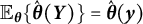
 $\mathbb {E}_{\boldsymbol {\theta }^{*}}\{\hat {\boldsymbol {\theta }}(\boldsymbol {Y})\}$
is unknown, we approximate it with its unbiased estimate
$\mathbb {E}_{\boldsymbol {\theta }^{*}}\{\hat {\boldsymbol {\theta }}(\boldsymbol {Y})\}$
is unknown, we approximate it with its unbiased estimate
 $\hat {\boldsymbol {\theta }}(\boldsymbol {y})$
, where
$\hat {\boldsymbol {\theta }}(\boldsymbol {y})$
, where
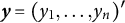 $\boldsymbol {y} = (y_{1}, \ldots , y_{n})'$
denotes a specific realization (or observed counterpart) of the random sample
$\boldsymbol {y} = (y_{1}, \ldots , y_{n})'$
denotes a specific realization (or observed counterpart) of the random sample
 $\boldsymbol {Y}$
. Then, if we can find a
$\boldsymbol {Y}$
. Then, if we can find a
 $\boldsymbol {\theta }$
such that
$\boldsymbol {\theta }$
such that
 $\mathbb {E}_{\boldsymbol {\theta }}\{\hat {\boldsymbol {\theta }}(\boldsymbol {Y})\} = \hat {\boldsymbol {\theta }}(\boldsymbol {y})$
, we can infer that this
$\mathbb {E}_{\boldsymbol {\theta }}\{\hat {\boldsymbol {\theta }}(\boldsymbol {Y})\} = \hat {\boldsymbol {\theta }}(\boldsymbol {y})$
, we can infer that this
 $\boldsymbol {\theta }$
should be close to
$\boldsymbol {\theta }$
should be close to
 $\boldsymbol {\theta }^{*}$
. Thus, the goal of bias correction becomes solving for
$\boldsymbol {\theta }^{*}$
. Thus, the goal of bias correction becomes solving for
 $\boldsymbol {\theta }$
from the following equation:
$\boldsymbol {\theta }$
from the following equation:
 $$ \begin{align} \mathbb{E}_{\boldsymbol{\theta}}\{\hat{\boldsymbol{\theta}}(\boldsymbol{Y})\} - \hat{\boldsymbol{\theta}}(\boldsymbol{y}) = \boldsymbol{0}. \end{align} $$
The solution to (5), denoted by
 $\tilde {\boldsymbol {\theta }}(\boldsymbol {y})$
, has been shown by Leung and Wang (Reference Leung and Wang1998) to reduce the bias to
$\tilde {\boldsymbol {\theta }}(\boldsymbol {y})$
, has been shown by Leung and Wang (Reference Leung and Wang1998) to reduce the bias to
 $O(n^{-1})$
for estimating single-parameter models under mild assumptions. In the Appendix, we generalize the bias-correction result in multiparameter settings, demonstrating that the bias-corrected estimator maintains the same
$O(n^{-1})$
for estimating single-parameter models under mild assumptions. In the Appendix, we generalize the bias-correction result in multiparameter settings, demonstrating that the bias-corrected estimator maintains the same
 $O(n^{-1})$
bias order and thus remains asymptotically unbiased.
$O(n^{-1})$
bias order and thus remains asymptotically unbiased.
The rationale behind this approach is illustrated in Figure 3, using the estimation of
 $\eta $
in the linear oscillator model as an example. We varied the true values of
$\eta $
in the linear oscillator model as an example. We varied the true values of
 $\eta $
from
$\eta $
from
 $-1$
to
$-1$
to
 $0$
(excluding
$0$
(excluding
 $0$
), and fixed the other parameters at the values used in the previous illustrative example to generated datasets. For each value of
$0$
), and fixed the other parameters at the values used in the previous illustrative example to generated datasets. For each value of
 $\eta $
, 10,000 datasets were generated, and
$\eta $
, 10,000 datasets were generated, and
 $\eta $
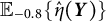
was estimated using GLLA. The expectation of
$\eta $
was estimated using GLLA. The expectation of
 $\eta $
(denoted by
$\eta $
(denoted by
 $\mathbb {E}_{\eta }\{\hat {\eta }(\boldsymbol {Y})\}$
) is plotted as a function of
$\mathbb {E}_{\eta }\{\hat {\eta }(\boldsymbol {Y})\}$
) is plotted as a function of
 $\eta $
in Figure 3 (the solid black line). The estimator
$\eta $
in Figure 3 (the solid black line). The estimator
 $\hat {\eta }(\boldsymbol {Y})$
is found to be biased, and the bias increases as the magnitude of
$\hat {\eta }(\boldsymbol {Y})$
is found to be biased, and the bias increases as the magnitude of
 $\eta $
increases. This trend is reflected in the deviation of
$\eta $
increases. This trend is reflected in the deviation of
 $\mathbb {E}_{\eta }\{\hat {\eta }(\boldsymbol {Y})\}$
from the diagonal (the dotted black line). For the true value of
$\mathbb {E}_{\eta }\{\hat {\eta }(\boldsymbol {Y})\}$
from the diagonal (the dotted black line). For the true value of
 $\eta = -0.8$
(indicated by the orange dashed line), GLLA overestimated the parameter (i.e.,
$\eta = -0.8$
(indicated by the orange dashed line), GLLA overestimated the parameter (i.e.,
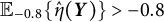 $\mathbb {E}_{-0.8}\{\hat {\eta }(\boldsymbol {Y})\}> -0.8$
). To correct the bias, we can use the biased estimator
$\mathbb {E}_{-0.8}\{\hat {\eta }(\boldsymbol {Y})\}> -0.8$
). To correct the bias, we can use the biased estimator
 $\hat {\eta }(\boldsymbol {Y})$
, whose sampling distribution is centered around
$\hat {\eta }(\boldsymbol {Y})$
, whose sampling distribution is centered around
 $\mathbb {E}_{-0.8}\{\hat {\eta }(\boldsymbol {Y})\}$
(depicted by the blue distribution), to obtain the sampling distribution for
$\mathbb {E}_{-0.8}\{\hat {\eta }(\boldsymbol {Y})\}$
(depicted by the blue distribution), to obtain the sampling distribution for
 $\tilde {\eta }(\boldsymbol {y})$
(the orange distribution) by identifying the corresponding x-coordinate from the solid black line. The sampling distribution of the bias-corrected estimator
$\tilde {\eta }(\boldsymbol {y})$
(the orange distribution) by identifying the corresponding x-coordinate from the solid black line. The sampling distribution of the bias-corrected estimator
 $\tilde {\eta }(\boldsymbol {y})$
is expected to center around the true value of
$\tilde {\eta }(\boldsymbol {y})$
is expected to center around the true value of
 $\eta = -0.8$
.
$\eta = -0.8$
.
Illustration of the bias-correction procedure using the
 $\eta $
estimation in the linear oscillator model as an example.
$\eta $
estimation in the linear oscillator model as an example.
Note: The solid black line represents the expectation
 $\mathbb {E}_{\eta }\{\hat {\eta }(\boldsymbol {Y})\}$
as a function of
$\mathbb {E}_{\eta }\{\hat {\eta }(\boldsymbol {Y})\}$
as a function of
 $\eta $
. The orange dashed line marks the true value of
$\eta $
. The orange dashed line marks the true value of
 $\eta = -0.8$
, and the blue and orange distributions show the sampling distributions of the biased estimator
$\eta = -0.8$
, and the blue and orange distributions show the sampling distributions of the biased estimator
 $\hat {\eta }(\boldsymbol {Y})$
and the bias-corrected estimator
$\hat {\eta }(\boldsymbol {Y})$
and the bias-corrected estimator
 $\tilde {\eta }(\boldsymbol {y})$
, respectively.
$\tilde {\eta }(\boldsymbol {y})$
, respectively.

2.1.2 Stochastic approximation and the Robbins–Monro algorithm
To solve Equation (5), SA methods can be used to obtain bias-corrected estimates. These methods are particularly well-suited for solving equations involving intractable expectations. Specifically, let
 $\boldsymbol {A}$
be a data-generating algorithm that produces simulated data
$\boldsymbol {A}$
be a data-generating algorithm that produces simulated data
 $\boldsymbol {Y}$
based on the parameter
$\boldsymbol {Y}$
based on the parameter
 $\boldsymbol {\theta }$
and a random variable
$\boldsymbol {\theta }$
and a random variable
 $\boldsymbol {U}$
with distribution
$\boldsymbol {U}$
with distribution
 $\mathbb {P}$
independent of
$\mathbb {P}$
independent of
 $\boldsymbol {\theta }$
, that is,
$\boldsymbol {\theta }$
, that is,
 $\boldsymbol {Y} = A(\boldsymbol {\theta }, \boldsymbol {U})$
. Consider solving for
$\boldsymbol {Y} = A(\boldsymbol {\theta }, \boldsymbol {U})$
. Consider solving for
 $\boldsymbol {\theta }$
from the equation (or a set of equations)
$\boldsymbol {\theta }$
from the equation (or a set of equations)
 $$ \begin{align} \boldsymbol{0} = \boldsymbol{g}(\boldsymbol{\theta}) = \mathbb{E}\{\boldsymbol{G}(\boldsymbol{\theta}, \boldsymbol{U})\}, \end{align} $$
where
 $\boldsymbol {g}(\boldsymbol {\theta }) = \mathbb {E}\{\hat {\boldsymbol {\theta }}[\boldsymbol {A}(\boldsymbol {\theta }, \boldsymbol {U})] \} - \hat {\boldsymbol {\theta }}(\boldsymbol {y})$
and
$\boldsymbol {g}(\boldsymbol {\theta }) = \mathbb {E}\{\hat {\boldsymbol {\theta }}[\boldsymbol {A}(\boldsymbol {\theta }, \boldsymbol {U})] \} - \hat {\boldsymbol {\theta }}(\boldsymbol {y})$
and
 $\boldsymbol {G}(\boldsymbol {\theta }, \boldsymbol {U}) = \hat {\boldsymbol {\theta }}[\boldsymbol {A}(\boldsymbol {\theta }, \boldsymbol {U})] - \hat {\boldsymbol {\theta }}(\boldsymbol {y})$
. The expectation is taken over the random variable
$\boldsymbol {G}(\boldsymbol {\theta }, \boldsymbol {U}) = \hat {\boldsymbol {\theta }}[\boldsymbol {A}(\boldsymbol {\theta }, \boldsymbol {U})] - \hat {\boldsymbol {\theta }}(\boldsymbol {y})$
. The expectation is taken over the random variable
 $\boldsymbol {U} \sim \mathbb {P}$
while the observed data
$\boldsymbol {U} \sim \mathbb {P}$
while the observed data
 $\boldsymbol {y}$
are kept fixed. In the previously discussed example based on the linear oscillator model, the frequency parameter
$\boldsymbol {y}$
are kept fixed. In the previously discussed example based on the linear oscillator model, the frequency parameter
 $\eta $
can be viewed as the parameter
$\eta $
can be viewed as the parameter
 $\boldsymbol {\theta }$
, and the measurement error
$\boldsymbol {\theta }$
, and the measurement error
 $e(t)$
can be interpreted as parameter-free random components
$e(t)$
can be interpreted as parameter-free random components
 $\boldsymbol {U}$
.Footnote
6
$\boldsymbol {U}$
.Footnote
6
To solve Equation (6), a fundamental SA method—the Robbins–Monro algorithm (RM algorithm; Robbins & Monro, Reference Robbins and Monro1951)—can be applied. This algorithm iteratively updates the approximation to the root using the following recursive scheme:
 $$ \begin{align} \boldsymbol{\theta}_{k+1} = \boldsymbol{\theta}_{k} - \gamma_{k}\hat{\boldsymbol{g}}_{m}(\boldsymbol{\theta}_{k}), \end{align} $$
where
 $\boldsymbol {\theta }_{k}$
denotes the k-th iterate (
$\boldsymbol {\theta }_{k}$
denotes the k-th iterate (
 $k = 1, 2, \ldots , K$
; K is the total number of iterations) of
$k = 1, 2, \ldots , K$
; K is the total number of iterations) of
 $\boldsymbol {\theta }$
,
$\boldsymbol {\theta }$
,
 $\gamma _{k}$
is a sequence of constants converging to zero, and
$\gamma _{k}$
is a sequence of constants converging to zero, and
 $\hat {\boldsymbol {g}}_{m}(\boldsymbol {\theta }_{k})$
is an unbiased Monte Carlo (MC) estimate of
$\hat {\boldsymbol {g}}_{m}(\boldsymbol {\theta }_{k})$
is an unbiased Monte Carlo (MC) estimate of
 $\boldsymbol {g}(\boldsymbol {\theta }_{k})$
, which is computed as
$\boldsymbol {g}(\boldsymbol {\theta }_{k})$
, which is computed as
 $$ \begin{align} \hat{\boldsymbol{g}}_{m}(\boldsymbol{\theta}_{k}) = \frac{1}{m} \sum_{j=1}^{m} \boldsymbol{G}(\boldsymbol{\theta}_{k}, \boldsymbol{U}_{j}). \end{align} $$
Here,
 $\boldsymbol {U}_{1}, \ldots , \boldsymbol {U}_{m}$
are independent and identically distributed samples drawn from
$\boldsymbol {U}_{1}, \ldots , \boldsymbol {U}_{m}$
are independent and identically distributed samples drawn from
 $\mathbb {P}$
, and m is the total number of MC simulations (which is typically not large in practice). In this study, we set
$\mathbb {P}$
, and m is the total number of MC simulations (which is typically not large in practice). In this study, we set
 $m = 5$
for all simulations and the empirical example.
$m = 5$
for all simulations and the empirical example.
The sequence
 $\gamma _{k}$
must satisfy the following conditions to ensure convergence of the algorithm:
$\gamma _{k}$
must satisfy the following conditions to ensure convergence of the algorithm:
 $$ \begin{align} \gamma_{k} \in (0, 1], \quad \sum_{k=1}^{\infty}\gamma_{k} = \infty, \quad \text{and} \quad \sum_{k=1}^{\infty}\gamma_{k}^{2} < \infty. \end{align} $$
These conditions ensure that
 $\gamma _{k}$
decreases slowly to zero, allowing the algorithm to filter out the noise effect and ensuring that the sequence of estimates converges to the root of
$\gamma _{k}$
decreases slowly to zero, allowing the algorithm to filter out the noise effect and ensuring that the sequence of estimates converges to the root of
 $\boldsymbol {g}(\cdot )$
. In this study, we set
$\boldsymbol {g}(\cdot )$
. In this study, we set
 $\gamma _{k} = \alpha k^{-\beta }$
with some
$\gamma _{k} = \alpha k^{-\beta }$
with some
 $\alpha> 0$
and
$\alpha> 0$
and
 $\beta \in (\frac {1}{2}, 1]$
, ensuring that the constants decrease slowly to zero.
$\beta \in (\frac {1}{2}, 1]$
, ensuring that the constants decrease slowly to zero.
2.2 Illustrative example
2.2.1 Procedure of bias correction
The dataset generated based on the linear oscillator model is used to illustrate the bias-correction procedure of the two-stage GLLA estimates. For illustrative purposes, we focus on correcting the biased estimate of the frequency parameter
 $\eta $
. The RM algorithm takes the following steps to correct the biased estimates:
$\eta $
. The RM algorithm takes the following steps to correct the biased estimates:
-
Step 0: Initialize by setting
 $k = 0$
and obtaining the initial estimates
$\hat {\boldsymbol {\theta }}_0$
using GLLA. Set
$\boldsymbol {\theta }_1 = \hat {\boldsymbol {\theta }}_0$
.
$k = 0$
and obtaining the initial estimates
$\hat {\boldsymbol {\theta }}_0$
using GLLA. Set
$\boldsymbol {\theta }_1 = \hat {\boldsymbol {\theta }}_0$
. -
Step 1: Set
$k = k + 1$
. Generate
$\boldsymbol {U}_{1}, \dots , \boldsymbol {U}_{m}$
from
$\mathbb {P}$
and compute: (10)
$$ \begin{align} \hat{\boldsymbol{g}}_m(\boldsymbol{\theta}_k) = \frac{1}{m}\sum_{j = 1}^m\hat{\boldsymbol{\theta}}[\boldsymbol{A}(\boldsymbol{\theta}_k,\boldsymbol{U}_j)] - \hat{\boldsymbol{\theta}}(\boldsymbol{y}). \end{align} $$
When generating datasets, the initial values of the displacement (
$x_{1}$
) and the first derivative (
$\dot {x}_{1}$
) are fixed to their values used in the previous simulation illustration for simplicity. -
Step 2: Update
$\boldsymbol {\theta }_{k}$
using Equation (7), with
$\alpha = 0.3$
,
$\beta = 0.6$
for all simulations in this study. -
Step 3: Repeat Steps 1 and 2 until convergence.


The final point estimates after a sufficiently large number of iterations K are obtained using the weighted average
 $$ \begin{align} \overline{\boldsymbol{\theta}}_{K} = \frac{\sum_{k=\lfloor K/2 \rfloor + 1}^{K}\gamma_{k}\boldsymbol{\theta}_{k}}{\sum_{k=\lfloor K/2 \rfloor + 1}^{K}\gamma_{k}}, \end{align} $$
where
 $\lfloor \cdot \rfloor $
denotes the integer part of a real number. In this study, we run a fixed total of 5,000 iterations. Convergence was considered achieved if the relative difference between the point estimates at iterations 4,999 and 5,000 (i.e., their difference divided by the estimate at 4,999) fell below a tolerance threshold of 0.01%.
$\lfloor \cdot \rfloor $
denotes the integer part of a real number. In this study, we run a fixed total of 5,000 iterations. Convergence was considered achieved if the relative difference between the point estimates at iterations 4,999 and 5,000 (i.e., their difference divided by the estimate at 4,999) fell below a tolerance threshold of 0.01%.
Additionally, the SE of the frequency parameter was estimated using the following equation (the derivation of a more general form is provided in the Appendix as Equation (16); Equation (12) is a special case of Equation (16)):
 $$ \begin{align} \widehat{SE} = \sqrt{[\widehat{\dot{\boldsymbol{L}}}(\overline{\boldsymbol{\theta}}_{K})]^{-2} \widehat{\mathrm{Var}}_{\overline{\boldsymbol{\theta}}_{K}}\{\hat{\boldsymbol{\theta}}\}}, \end{align} $$
where
 $\widehat {\mathrm {Var}}_{\overline {\boldsymbol {\theta }}_{K}}\{\hat {\boldsymbol {\theta }}\}$
was estimated using the MC approximation with 10,000 simulations. The expected value
$\widehat {\mathrm {Var}}_{\overline {\boldsymbol {\theta }}_{K}}\{\hat {\boldsymbol {\theta }}\}$
was estimated using the MC approximation with 10,000 simulations. The expected value
 $\mathbb {E}_{\boldsymbol {\theta }}\{\hat {\boldsymbol {\theta }}\}$
is denoted as
$\mathbb {E}_{\boldsymbol {\theta }}\{\hat {\boldsymbol {\theta }}\}$
is denoted as
 $\boldsymbol {L}(\boldsymbol {\theta })$
, and
$\boldsymbol {L}(\boldsymbol {\theta })$
, and
 $\widehat {\dot {\boldsymbol {L}}}(\overline {\boldsymbol {\theta }}_{K})$
is its derivative evaluated at the final point estimate
$\widehat {\dot {\boldsymbol {L}}}(\overline {\boldsymbol {\theta }}_{K})$
is its derivative evaluated at the final point estimate
 $\overline {\boldsymbol {\theta }}_{K}$
. This derivative was computed numerically using the finite differences method with the jacobian function in the R package numDeriv (Gilbert & Varadhan, Reference Gilbert and Varadhan2016), where we fixed the parameter-free random components
$\overline {\boldsymbol {\theta }}_{K}$
. This derivative was computed numerically using the finite differences method with the jacobian function in the R package numDeriv (Gilbert & Varadhan, Reference Gilbert and Varadhan2016), where we fixed the parameter-free random components
 $\boldsymbol {U}$
to ensure numerical variability arises solely from parameter perturbations. This approach is also applied in the computation of the more general form of SE described later. For notational simplicity, from Equation (12) onward, we omit explicit dependence notation in estimators.
$\boldsymbol {U}$
to ensure numerical variability arises solely from parameter perturbations. This approach is also applied in the computation of the more general form of SE described later. For notational simplicity, from Equation (12) onward, we omit explicit dependence notation in estimators.
2.2.2 Results
Figure 4 displays the iterates of
 $\eta $
using the bias-correction method. Although starting from the highly biased GLLA estimate (
$\eta $
using the bias-correction method. Although starting from the highly biased GLLA estimate (
 $\hat {\eta } = -0.618$
), the iterates gradually converged, with the final estimate (
$\hat {\eta } = -0.618$
), the iterates gradually converged, with the final estimate (
 $\overline {\eta }_{K} = -0.800$
) after
$\overline {\eta }_{K} = -0.800$
) after
 $K = 1,000$
iterations matching the true value to the third decimal place. This result demonstrates the effectiveness of the bias-correction procedure in reducing bias in the two-stage GLLA estimates in differential equation models. In addition, the SE estimate for
$K = 1,000$
iterations matching the true value to the third decimal place. This result demonstrates the effectiveness of the bias-correction procedure in reducing bias in the two-stage GLLA estimates in differential equation models. In addition, the SE estimate for
 $\eta $
was
$\eta $
was
 $0.169 \times 10^{-3}$
, indicating high precision in the final estimate.
$0.169 \times 10^{-3}$
, indicating high precision in the final estimate.
Iterates and point estimates of
 $\eta $
in the linear oscillator model.
$\eta $
in the linear oscillator model.
Note: The solid line represents the iterates of
 $\eta $
using the bias-correction method. The dashed lines indicate the true value (orange), the point estimates using GLLA (blue), and the point estimate using LDE (teal).
$\eta $
using the bias-correction method. The dashed lines indicate the true value (orange), the point estimates using GLLA (blue), and the point estimate using LDE (teal).

2.2.3 Summary
This example illustrates the bias-correction procedure in a relatively simple setting, where (a) only one parameter is of focus (i.e., the frequency parameter
 $\eta $
in the linear oscillator model) and (b) the model involves only time-independent noise (i.e., measurement error). To assess the performance of the bias-correction method in more general settings, the remainder of this article will extend the approach to the damped linear oscillator model, (a) addressing bias correction and SE estimation for multiple parameters and (b) incorporating time-dependent process noise (i.e., dynamic error) into the model.
$\eta $
in the linear oscillator model) and (b) the model involves only time-independent noise (i.e., measurement error). To assess the performance of the bias-correction method in more general settings, the remainder of this article will extend the approach to the damped linear oscillator model, (a) addressing bias correction and SE estimation for multiple parameters and (b) incorporating time-dependent process noise (i.e., dynamic error) into the model.
3 Extension to the damped linear oscillator model
The damped linear oscillator model is a widely used differential equation model in psychological research (e.g., Chow et al., Reference Chow, Ram, Boker, Fujita and Clore2005; Ollero et al., Reference Ollero, Estrada, Hunter and Cáncer2025; Hu & Treinen, Reference Hu and Treinen2019). In this section, we first demonstrate how the bias-correction procedure can be applied to reduce bias in the estimation of multiple parameters in the damped linear oscillator model. We then further evaluate the effectiveness of the bias-correction method by incorporating dynamic error into the model.
3.1 Bias correction for multiple parameters in the damped linear oscillator model
The damped linear oscillator model with measurement error is specified as follows:
 $$ \begin{align} \!\!\!X(t) = x(t) + e(t),\quad \end{align} $$
 $$ \begin{align} \ddot{x}(t) = \eta x(t) + \zeta\dot{x}(t). \end{align} $$
Equation (13) is the same as Equation (1). In Equation (14),
 $\dot {x}(t)$
and
$\dot {x}(t)$
and
 $\ddot {x}(t)$
represent the first and second derivatives of
$\ddot {x}(t)$
represent the first and second derivatives of
 $x(t)$
with respect to time, respectively. The frequency parameter
$x(t)$
with respect to time, respectively. The frequency parameter
 $\eta $
describes the frequency of oscillation. The damping parameter
$\eta $
describes the frequency of oscillation. The damping parameter
 $\zeta $
governs the amplitude of oscillation.Footnote
7
A negative value of
$\zeta $
governs the amplitude of oscillation.Footnote
7
A negative value of
 $\zeta $
indicates a decrease in oscillation amplitude over time, while a positive value of
$\zeta $
indicates a decrease in oscillation amplitude over time, while a positive value of
 $\zeta $
indicates an increase in amplitude. When
$\zeta $
indicates an increase in amplitude. When
 $\zeta =0$
, the oscillation amplitude remains constant, and the model reduces to the linear oscillator model.
$\zeta =0$
, the oscillation amplitude remains constant, and the model reduces to the linear oscillator model.
3.1.1 Data generation
To preliminarily assess the effectiveness of the bias-correction method for GLLA estimates of multiple parameters, we generated a large dataset based on the damped linear oscillator model, in which the frequency parameter, damping parameter, standard deviation of measurement error, and initial values were all treated as unknown parameters to be estimated. Specifically, individual time-series data (
 $T = 100$
) were generated according to Equations (13) and (14) for
$T = 100$
) were generated according to Equations (13) and (14) for
 $N = 1,000$
individuals. The measurement error-free data were first simulated using the analytic solution of Equation (14), which is valid when
$N = 1,000$
individuals. The measurement error-free data were first simulated using the analytic solution of Equation (14), which is valid when
 $\eta <0$
and
$\eta <0$
and
 $\zeta ^2+4\eta <0$
(Hu & Treinen, Reference Hu and Treinen2019):
$\zeta ^2+4\eta <0$
(Hu & Treinen, Reference Hu and Treinen2019):
 $$ \begin{align} x(t) = e^{\zeta t/2}\left(A\cos ( \omega^{\prime}t ) + B\sin{( \omega^{\prime}t )} \right), \end{align} $$
where
 $\omega ^{\prime} = \sqrt {- \eta - \zeta ^{2}/4}$
,
$\omega ^{\prime} = \sqrt {- \eta - \zeta ^{2}/4}$
,
 $A = x_{1}$
, and
$A = x_{1}$
, and
 $B = {\dot {x}}_{1}/\omega ^{\prime}$
, with
$B = {\dot {x}}_{1}/\omega ^{\prime}$
, with
 $x_{1}$
and
$x_{1}$
and
 ${\dot {x}}_{1}$
representing the initial values of the displacement and the first derivative, respectively. We set
${\dot {x}}_{1}$
representing the initial values of the displacement and the first derivative, respectively. We set
 $\eta = -0.8$
and
$\eta = -0.8$
and
 $\zeta = -0.04$
to reflect a typical cycle length of 7 time points (i.e.,
$\zeta = -0.04$
to reflect a typical cycle length of 7 time points (i.e.,
 $2\pi /\omega ^{\prime} = 2\pi /\sqrt {- \eta - \zeta ^{2}/4} \approx 7$
) and a commonly small value of
$2\pi /\omega ^{\prime} = 2\pi /\sqrt {- \eta - \zeta ^{2}/4} \approx 7$
) and a commonly small value of
 $\zeta $
(Cho et al., Reference Cho, Chow, Marini and Martire2024).
$\zeta $
(Cho et al., Reference Cho, Chow, Marini and Martire2024).
When estimating derivatives using a five-dimensional time-delay embedded matrix via GLLA (see Figure 1), the first row of the resulting matrix represents the derivative estimates at the third time point of the original time series. Therefore, we set the values of the third time point for the zero- and first-order derivatives (
 $x_{3} = -10$
and
$x_{3} = -10$
and
 ${\dot {x}}_{3} = -10$
) in order to approximate the time series starting near a positive peak of the oscillation while simultaneously obtaining the true initial values for GLLA. We then used these values as initial conditions to generate (
${\dot {x}}_{3} = -10$
) in order to approximate the time series starting near a positive peak of the oscillation while simultaneously obtaining the true initial values for GLLA. We then used these values as initial conditions to generate (
 $T - 2$
) time points forward and 2 time points backward according to Equation (15), resulting in T time points for each individual. The observed dataset for each individual was generated by adding measurement error drawn from a normal distribution with mean zero and the standard deviation of
$T - 2$
) time points forward and 2 time points backward according to Equation (15), resulting in T time points for each individual. The observed dataset for each individual was generated by adding measurement error drawn from a normal distribution with mean zero and the standard deviation of
 $\sigma _{e} = 1$
. This generating process was repeated N times, yielding a final dataset with N individuals, each having T observations.
$\sigma _{e} = 1$
. This generating process was repeated N times, yielding a final dataset with N individuals, each having T observations.
3.1.2 Estimation and bias correction
To obtain the GLLA estimates of parameters in the damped linear oscillator model, we first estimated the zero-, first-, and second-order derivatives using a five-dimensional time-delay embedded matrix. We then fitted a linear regression model with the zero- and first-order derivatives as predictors and the second-order derivative as the outcome variable to estimate the frequency parameter
 $\eta $
and the damping parameter
$\eta $
and the damping parameter
 $\zeta $
. To estimate the third time point for the zero-order (
$\zeta $
. To estimate the third time point for the zero-order (
 $x_{3}$
) and first-order (
$x_{3}$
) and first-order (
 ${\dot {x}}_{3}$
) derivatives, we averaged the first row of the corresponding derivative estimates across individuals. For the standard deviation of measurement error, we used the between-person standard deviation of the first row of the zero-order derivative as an estimate.
${\dot {x}}_{3}$
) derivatives, we averaged the first row of the corresponding derivative estimates across individuals. For the standard deviation of measurement error, we used the between-person standard deviation of the first row of the zero-order derivative as an estimate.
To obtain the bias-corrected estimates, we followed the same procedure as in the linear oscillator model, except that in Step 1, five parameters (
 $\eta $
,
$\eta $
,
 $\zeta $
,
$\zeta $
,
 $x_{3}$
,
$x_{3}$
,
 ${\dot {x}}_{3}$
, and
${\dot {x}}_{3}$
, and
 $\sigma _{e}$
) were estimated and used to generate datasets during each iteration. The final point estimate for each parameter was calculated using Equation (11). The SE estimates were computed as
$\sigma _{e}$
) were estimated and used to generate datasets during each iteration. The final point estimate for each parameter was calculated using Equation (11). The SE estimates were computed as
 $$ \begin{align} \widehat{SE} = \sqrt{Diag(\widehat{\boldsymbol{\Sigma}})}, \end{align} $$
where the covariance matrix
 $\widehat {\boldsymbol {\Sigma }}$
is approximated by (the derivation is provided in the Appendix)
$\widehat {\boldsymbol {\Sigma }}$
is approximated by (the derivation is provided in the Appendix)
 $$ \begin{align} \widehat{\boldsymbol{\Sigma}} = \left[ \widehat{\dot{\boldsymbol{L}}}\left( {\overline{\boldsymbol{\theta}}}_{K} \right) \right]^{-1} {\widehat{\mathrm{Cov}}}_{{\overline{\boldsymbol{\theta}}}_{K}}\left\{ \widehat{\boldsymbol{\theta}} \right\} \left[ {\widehat{\dot{\boldsymbol{L}}}\left( {\overline{\boldsymbol{\theta}}}_{K} \right)} \right]^{-\top}. \end{align} $$
The covariance matrix
 ${\widehat {\mathrm {Cov}}}_{{\overline {\boldsymbol {\theta }}}_{K}}\left \{ \widehat {\boldsymbol {\theta }} \right \}$
was estimated using MC approximation with 10,000 simulations, and the Jacobian matrix
${\widehat {\mathrm {Cov}}}_{{\overline {\boldsymbol {\theta }}}_{K}}\left \{ \widehat {\boldsymbol {\theta }} \right \}$
was estimated using MC approximation with 10,000 simulations, and the Jacobian matrix
 $\widehat {\dot {\boldsymbol {L}}}\left ( {\overline {\boldsymbol {\theta }}}_{K} \right )$
was computed using the finite differences method.
$\widehat {\dot {\boldsymbol {L}}}\left ( {\overline {\boldsymbol {\theta }}}_{K} \right )$
was computed using the finite differences method.
For comparison, we also estimated the model parameters using state-space modeling (SSM) implemented in the R package dynr (Ou et al., Reference Ou, Hunter and Chow2019). The initial values for the frequency parameter
 $\eta $
and damping parameter
$\eta $
and damping parameter
 $\zeta $
were set to the GLLA estimates, while the initial value for the measurement error standard deviation
$\zeta $
were set to the GLLA estimates, while the initial value for the measurement error standard deviation
 $\sigma _e$
was set to the between-person standard deviation of the first row of the zero-order derivative estimates, consistent with the approach used for GLLA and the bias-correction method. For the initial conditions, which in dynr correspond to the first time point of the latent states (i.e., the zero- and first-order derivatives), we used the sample means across individuals of the first time point values for the zero-order derivative, and the mean of the numerical derivatives between the first and second time points for the first-order derivative. Given that the SSM estimates initial conditions at the first time point, whereas the bias-correction method estimates them at the third time point, a direct comparison of these initial condition parameters is not feasible. We imposed appropriate boundary constraints, restricting
$\sigma _e$
was set to the between-person standard deviation of the first row of the zero-order derivative estimates, consistent with the approach used for GLLA and the bias-correction method. For the initial conditions, which in dynr correspond to the first time point of the latent states (i.e., the zero- and first-order derivatives), we used the sample means across individuals of the first time point values for the zero-order derivative, and the mean of the numerical derivatives between the first and second time points for the first-order derivative. Given that the SSM estimates initial conditions at the first time point, whereas the bias-correction method estimates them at the third time point, a direct comparison of these initial condition parameters is not feasible. We imposed appropriate boundary constraints, restricting
 $\sigma _e> 0$
and
$\sigma _e> 0$
and
 $\eta < 0$
. All other estimation settings were kept at their default values.
$\eta < 0$
. All other estimation settings were kept at their default values.
3.1.3 Results
Figure 5 shows the iterates of parameters using the bias-correction method. All parameter iterates converged to equilibrium within 5,000 iterations. Compared to the GLLA estimates, the biased-corrected estimates were much closer to the true values, and exhibited small SE estimates (see Table 1). The SSM estimates for the frequency parameter
 $\eta $
and the measurement error standard deviation
$\eta $
and the measurement error standard deviation
 $\sigma _e$
were also highly accurate. However, for the damping parameter
$\sigma _e$
were also highly accurate. However, for the damping parameter
 $\zeta $
, the SSM estimate exhibited substantial bias, which was even larger than that of the GLLA estimate. This suggests that the bias-correction method effectively reduces the bias of the GLLA estimates for multiple parameters in the damped linear oscillator model with only time-independent noise (i.e., measurement error). This result motivates further investigation into the performance of the bias-correction method when time-dependent dynamic error is introduced into the model.
$\zeta $
, the SSM estimate exhibited substantial bias, which was even larger than that of the GLLA estimate. This suggests that the bias-correction method effectively reduces the bias of the GLLA estimates for multiple parameters in the damped linear oscillator model with only time-independent noise (i.e., measurement error). This result motivates further investigation into the performance of the bias-correction method when time-dependent dynamic error is introduced into the model.
Parameter estimates in the damped linear oscillator model with and without dynamic error using GLLA, state-space modeling (SSM), and the bias-correction method

Note:
 $^a$
The values of 0.000 are a result of rounding to three decimal places. When rounded to four decimal places, the values are 0.0001.
$^a$
The values of 0.000 are a result of rounding to three decimal places. When rounded to four decimal places, the values are 0.0001.
Relative bias of the parameter estimates and iterates in the damped linear oscillator model.
Note: The solid line represents the iterates of parameters using the bias-correction method. The dashed lines indicate the true value (orange), the GLLA estimates (dark blue), and the SSM estimates (light blue).

3.2 Bias correction in the damped linear oscillator model with dynamic error
The damped linear oscillator model with both time-independent measurement error and time-dependent dynamic error can be expressed as follows:
 $$ \begin{align} X(t) &= x(t) + e(t), \end{align} $$

Equation (18) is identical to Equations (1) and (13). In Equation (19), the original damped linear oscillator model in Equation (14) is multiplied by
 $\Delta t$
with the addition of the change in dynamic error
$\Delta t$
with the addition of the change in dynamic error
 $\Delta \varepsilon (t)$
, resulting in a stochastic version of the model.Footnote
8
The change in dynamic error
$\Delta \varepsilon (t)$
, resulting in a stochastic version of the model.Footnote
8
The change in dynamic error
 $\Delta \varepsilon (t)$
over a short time interval
$\Delta \varepsilon (t)$
over a short time interval
 $[t,t + \Delta t]$
follows a normal distribution with mean zero and variance
$[t,t + \Delta t]$
follows a normal distribution with mean zero and variance
 $\sigma _{\varepsilon }^{2}\Delta t$
. In other words,
$\sigma _{\varepsilon }^{2}\Delta t$
. In other words,
 $\Delta \varepsilon (t)$
can be modeled as the increment of a univariate standard Wiener process
$\Delta \varepsilon (t)$
can be modeled as the increment of a univariate standard Wiener process
 $W(t)$
scaled by the standard deviation
$W(t)$
scaled by the standard deviation
 $\sigma _{\varepsilon }$
, such that
$\sigma _{\varepsilon }$
, such that
 $\Delta \varepsilon (t) = \sigma _{\varepsilon }\Delta W(t)$
, where
$\Delta \varepsilon (t) = \sigma _{\varepsilon }\Delta W(t)$
, where
 $\Delta W(t) = W(t + \Delta t) - W(t)$
follows a normal distribution with mean zero and variance of
$\Delta W(t) = W(t + \Delta t) - W(t)$
follows a normal distribution with mean zero and variance of
 $\Delta t$
(i.e.,
$\Delta t$
(i.e.,
 $\Delta W(t) \sim N(0,\Delta t)$
).
$\Delta W(t) \sim N(0,\Delta t)$
).
Although both dynamic error
 $\varepsilon (t)$
and measurement error
$\varepsilon (t)$
and measurement error
 $e(t)$
follow normal distributions, they serve fundamentally different roles in the model. The dynamic error captures stochastic shocks that continuously influence the current and future states of the dynamic system, while the measurement error represents noise that only affects the current state (i.e., the measurement occasion) of the system (Chen et al., Reference Chen, Chow, Hunter, Montfort, Oud and Voelkle2018). In psychological studies that use differential equation models to examine dynamic processes, incorporating dynamic error is a more realistic assumption. This assumption reflects that the current state of the dynamic system cannot be perfectly predicted by its previous state, as random noise can contribute to the dynamic process at any moment (Ollero et al., Reference Ollero, Estrada, Hunter and Cáncer2025). Moreover, it accounts for the impact of unknown or unmodeled factors on the system’s evolution.
$e(t)$
follow normal distributions, they serve fundamentally different roles in the model. The dynamic error captures stochastic shocks that continuously influence the current and future states of the dynamic system, while the measurement error represents noise that only affects the current state (i.e., the measurement occasion) of the system (Chen et al., Reference Chen, Chow, Hunter, Montfort, Oud and Voelkle2018). In psychological studies that use differential equation models to examine dynamic processes, incorporating dynamic error is a more realistic assumption. This assumption reflects that the current state of the dynamic system cannot be perfectly predicted by its previous state, as random noise can contribute to the dynamic process at any moment (Ollero et al., Reference Ollero, Estrada, Hunter and Cáncer2025). Moreover, it accounts for the impact of unknown or unmodeled factors on the system’s evolution.
3.2.1 Data generation
To generate data for the damped linear oscillator model with dynamic error, we first simulate the measurement-error-free time-series data for each individual using the Euler method for numerical integration. This method approximates the state of the system over discrete time steps with the following update rules:
 $$ \begin{align} x(t + \Delta t) &= x(t) + \dot{x}(t) \Delta t, \end{align} $$

where the time step size is
 $\Delta t = 0.01$
. The initial conditions for the zero- and first-order derivatives were set at the third time point (
$\Delta t = 0.01$
. The initial conditions for the zero- and first-order derivatives were set at the third time point (
 $x_{3}$
and
$x_{3}$
and
 ${\dot {x}}_{3}$
). Numerical integration was used to generate
${\dot {x}}_{3}$
). Numerical integration was used to generate
 $(T - 2)/\Delta t$
time points forward and
$(T - 2)/\Delta t$
time points forward and
 $2/\Delta t$
time points backward, where
$2/\Delta t$
time points backward, where
 $T = 1,000$
, resulting in a total of
$T = 1,000$
, resulting in a total of
 $T/\Delta t = 100,000$
states. A thinning interval of
$T/\Delta t = 100,000$
states. A thinning interval of
 $1/\Delta t$
was then applied, resulting in
$1/\Delta t$
was then applied, resulting in
 $T = 1,000$
data points for each individual. The observed dataset for each individual was generated by adding measurement error drawn from a normal distribution with mean zero and standard deviation
$T = 1,000$
data points for each individual. The observed dataset for each individual was generated by adding measurement error drawn from a normal distribution with mean zero and standard deviation
 $\sigma _{e}$
. This process was repeated
$\sigma _{e}$
. This process was repeated
 $N = 100$
times, yielding a final dataset with N individuals, each having T observations. The true values of parameters were set to the same values used in the previous simulation (
$N = 100$
times, yielding a final dataset with N individuals, each having T observations. The true values of parameters were set to the same values used in the previous simulation (
 $\eta = -0.8$
,
$\eta = -0.8$
,
 $\zeta = -0.04$
,
$\zeta = -0.04$
,
 $x_{3} = -10$
,
$x_{3} = -10$
,
 ${\dot {x}}_{3} = -10$
, and
${\dot {x}}_{3} = -10$
, and
 $\sigma _{e} = 1$
), and the standard deviation of the dynamic error was set to
$\sigma _{e} = 1$
), and the standard deviation of the dynamic error was set to
 $\sigma _{\varepsilon } = 0.5$
.
$\sigma _{\varepsilon } = 0.5$
.
3.2.2 Estimation and bias correction
The GLLA estimates of the parameters
 $\eta $
,
$\eta $
,
 $\zeta $
,
$\zeta $
,
 $x_{3}$
,
$x_{3}$
,
 ${\dot {x}}_{3}$
, and
${\dot {x}}_{3}$
, and
 $\sigma _{e}$
were obtained using the same method as in the previous section. Additionally, the standard deviation of dynamic error
$\sigma _{e}$
were obtained using the same method as in the previous section. Additionally, the standard deviation of dynamic error
 $\sigma _{\varepsilon }$
was estimated using the residual standard deviation from the linear regression of the zero- and first-order derivatives on the second-order derivative. The bias-corrected estimates were obtained for all six parameters (
$\sigma _{\varepsilon }$
was estimated using the residual standard deviation from the linear regression of the zero- and first-order derivatives on the second-order derivative. The bias-corrected estimates were obtained for all six parameters (
 $\eta $
,
$\eta $
,
 $\zeta $
,
$\zeta $
,
 $x_{3}$
,
$x_{3}$
,
 ${\dot {x}}_{3}$
,
${\dot {x}}_{3}$
,
 $\sigma _{e}$
, and
$\sigma _{e}$
, and
 $\sigma _{\varepsilon }$
). The point estimates and SE estimates computed according to Equations (11) and (16), respectively.
$\sigma _{\varepsilon }$
). The point estimates and SE estimates computed according to Equations (11) and (16), respectively.
We also estimated the model parameters using SSM method. We specified the model following the example provided in the package documentation (https://github.com/mhunter1/dynr/blob/master/demo/LinearSDE.R). The initial values for the five parameters (
 $\eta $
,
$\eta $
,
 $\zeta $
,
$\zeta $
,
 $x_{3}$
,
$x_{3}$
,
 ${\dot {x}}_{3}$
, and
${\dot {x}}_{3}$
, and
 $\sigma _{e}$
) were set following the same procedure as described in the previous section for the model without dynamic error. For the dynamic error standard deviation
$\sigma _{e}$
) were set following the same procedure as described in the previous section for the model without dynamic error. For the dynamic error standard deviation
 $\sigma _{\varepsilon }$
, the initial value was set to the GLLA estimate, consistent with the approach used for the bias-correction method. We imposed boundary constraints, requiring
$\sigma _{\varepsilon }$
, the initial value was set to the GLLA estimate, consistent with the approach used for the bias-correction method. We imposed boundary constraints, requiring
 $\sigma _e> 0$
,
$\sigma _e> 0$
,
 $\sigma _{\varepsilon }> 0$
, and
$\sigma _{\varepsilon }> 0$
, and
 $\eta < 0$
.
$\eta < 0$
.
3.2.3 Results
Figure 6 presents the parameter iterates using the bias-correction method in the damped linear oscillator model with dynamic error. All parameters converged to their equilibrium within 5,000 iterations. As shown in Table 1, the GLLA estimates of the frequency parameter
 $\eta $
and the damping parameter
$\eta $
and the damping parameter
 $\zeta $
in the damped linear oscillator model with dynamic error exhibited larger bias than those in the model without dynamic error. The GLLA estimate of
$\zeta $
in the damped linear oscillator model with dynamic error exhibited larger bias than those in the model without dynamic error. The GLLA estimate of
 $\sigma _{\varepsilon }$
in the model with dynamic error also showed a large deviation from its true value. The SSM estimates for the frequency parameter
$\sigma _{\varepsilon }$
in the model with dynamic error also showed a large deviation from its true value. The SSM estimates for the frequency parameter
 $\eta $
and the measurement error standard deviation
$\eta $
and the measurement error standard deviation
 $\sigma _e$
showed acceptable bias levels. However, consistent with the results from the model without dynamic error, the SSM estimate for the damping parameter
$\sigma _e$
showed acceptable bias levels. However, consistent with the results from the model without dynamic error, the SSM estimate for the damping parameter
 $\zeta $
exhibited substantial bias that was larger than that of the GLLA estimate. Furthermore, the SSM estimate for the dynamic error standard deviation
$\zeta $
exhibited substantial bias that was larger than that of the GLLA estimate. Furthermore, the SSM estimate for the dynamic error standard deviation
 $\sigma _{\varepsilon }$
showed severe overestimation. For the biased-corrected estimates, although some still deviated slightly from their true values, the bias was largely reduced compared to the initial estimates using GLLA. The SE estimates were relatively larger than those in the damped linear oscillator model without dynamic error (except for the SE estimate of
$\sigma _{\varepsilon }$
showed severe overestimation. For the biased-corrected estimates, although some still deviated slightly from their true values, the bias was largely reduced compared to the initial estimates using GLLA. The SE estimates were relatively larger than those in the damped linear oscillator model without dynamic error (except for the SE estimate of
 $\sigma _{e}$
). These findings provide initial evidence for the effectiveness of the bias-correction method in addressing multiple parameters in a differential equation model with dynamic error.
$\sigma _{e}$
). These findings provide initial evidence for the effectiveness of the bias-correction method in addressing multiple parameters in a differential equation model with dynamic error.
Relative bias of the parameter estimates and iterates in the damped linear oscillator model with dynamic error.
Note: The solid line represents the iterates of parameters using the bias-correction method. The dashed lines indicate the true value (orange), the GLLA estimates (blue), and the SSM estimates (purple). The SSM point estimates (see Table 1) are not included in this figure to maintain clarity in visualization, as the large relative bias for
 $\sigma _{\varepsilon }$
would disproportionately scale the y-axis.
$\sigma _{\varepsilon }$
would disproportionately scale the y-axis.

4 Simulation study
Next, we conducted a simulation study to examine the effectiveness of the bias-correction method in the damped linear oscillator model with dynamic error. Specifically, we varied the true values of the damping parameter, the sample size, and the number of time points per individual, and compared the parameter estimates using GLLA, SSM, and the bias-correction method to assess their performance across different scenarios.
4.1 Procedure
We adopted the same procedure of data generation and parameter estimation as described in Section 3.2. In summary, we first simulated time series for each individual using the Euler method for numerical integration, and added measurement error to obtain observed data. This process was repeated for N individuals, each having T observations. For parameter estimation, we first constructed a five-dimensional time-delay embedded matrix and applied GLLA to estimate zero-, first-, and second-order derivatives. Using the estimated derivatives, we obtained the GLLA estimates of the six parameters (
 $\eta $
,
$\eta $
,
 $\zeta $
,
$\zeta $
,
 $x_{3}$
,
$x_{3}$
,
 ${\dot {x}}_{3}$
,
${\dot {x}}_{3}$
,
 $\sigma _{e}$
, and
$\sigma _{e}$
, and
 $\sigma _{\varepsilon }$
) in the damped linear oscillator model with dynamic error. Bias correction was performed using the RM algorithm outlined in Section 2.2.1. The point estimates were computed according to Equation (11), and the SE estimates were obtained using MC approximation and numerical differentiation method according to Equation (16). For comparison, we also estimated the parameters based on state-space models using the dynr package (Ou et al., Reference Ou, Hunter and Chow2019), following the same procedure as described in the previous section. The analysis was conducted in R 4.2.2 (R Core Team, 2020).
$\sigma _{\varepsilon }$
) in the damped linear oscillator model with dynamic error. Bias correction was performed using the RM algorithm outlined in Section 2.2.1. The point estimates were computed according to Equation (11), and the SE estimates were obtained using MC approximation and numerical differentiation method according to Equation (16). For comparison, we also estimated the parameters based on state-space models using the dynr package (Ou et al., Reference Ou, Hunter and Chow2019), following the same procedure as described in the previous section. The analysis was conducted in R 4.2.2 (R Core Team, 2020).
4.2 Simulation conditions
We varied the damping parameter (
 $\zeta $
=
$\zeta $
=
 $-$
0.04, 0, 0.04), the sample size (N = 50, 150, 500), and the number of time points per individual (T = 14, 28, 56), which were fully crossed, resulting in 27 (= 3
$-$
0.04, 0, 0.04), the sample size (N = 50, 150, 500), and the number of time points per individual (T = 14, 28, 56), which were fully crossed, resulting in 27 (= 3
 $\times $
3
$\times $
3
 $\times $
3) simulation conditions. In each condition, we replicated the MC simulation 500 times. The other parameters (
$\times $
3) simulation conditions. In each condition, we replicated the MC simulation 500 times. The other parameters (
 $\eta = -0.8$
,
$\eta = -0.8$
,
 $x_{3} = -10$
,
$x_{3} = -10$
,
 ${\dot {x}}_{3} = -10$
,
${\dot {x}}_{3} = -10$
,
 $\sigma _{e} = 1$
, and
$\sigma _{e} = 1$
, and
 $\sigma _{\varepsilon } = 0.5$
) were held constant across all simulation conditions. The frequency parameter
$\sigma _{\varepsilon } = 0.5$
) were held constant across all simulation conditions. The frequency parameter
 $\eta $
and the damping parameter
$\eta $
and the damping parameter
 $\zeta $
are of primary interest in the damped linear oscillator model. In the simulation study, we focused on
$\zeta $
are of primary interest in the damped linear oscillator model. In the simulation study, we focused on
 $\eta = -0.8$
to account for a typical cycle length of 7 time points (e.g., one week with one measurement per day), and varied
$\eta = -0.8$
to account for a typical cycle length of 7 time points (e.g., one week with one measurement per day), and varied
 $\zeta $
to represent a system with a damping process (
$\zeta $
to represent a system with a damping process (
 $\zeta < 0$
), an amplification process (
$\zeta < 0$
), an amplification process (
 $\zeta> 0$
), or without damping (
$\zeta> 0$
), or without damping (
 $\zeta = 0$
). For sample size, we used 50, 150, and 500 to represent small, medium, and large samples, respectively, as in typical intensive longitudinal studies. For the number of time points per individual, we chose 14, 28, and 56 to represent common study durations, covering approximately two, four (about one month), and eight (about two months) cycles.
$\zeta = 0$
). For sample size, we used 50, 150, and 500 to represent small, medium, and large samples, respectively, as in typical intensive longitudinal studies. For the number of time points per individual, we chose 14, 28, and 56 to represent common study durations, covering approximately two, four (about one month), and eight (about two months) cycles.
4.3 Evaluation criteria
4.3.1 Convergence rate
For the bias-correction method, we run a fixed total of 5,000 iterations. Convergence was determined by computing the relative difference between the point estimates at iterations 4,999 and 5,000 (i.e., their difference divided by the estimate at 4,999), with a tolerance threshold set to 0.01%.Footnote
9
For the converged cases of the bias-correction and SSM methods, we further examined the SE estimates to exclude outliers or improper solutions (i.e., SE estimates greater than 10 were considered outliers, as they were typically much less than 10). For the bias-correction method, we identified one and two cases containing outliers in the following two simulation conditions, respectively: (a)
 $N = 500$
,
$N = 500$
,
 $T = 56$
,
$T = 56$
,
 $\zeta = 0.04$
and (b)
$\zeta = 0.04$
and (b)
 $N = 50$
,
$N = 50$
,
 $T = 56$
,
$T = 56$
,
 $\zeta = 0$
. For the SSM method, we identified one and two cases containing outliers in the following two simulation conditions, respectively: (a)
$\zeta = 0$
. For the SSM method, we identified one and two cases containing outliers in the following two simulation conditions, respectively: (a)
 $N = 150$
,
$N = 150$
,
 $T = 14$
,
$T = 14$
,
 $\zeta = 0$
and (b)
$\zeta = 0$
and (b)
 $N = 150$
,
$N = 150$
,
 $T = 14$
,
$T = 14$
,
 $\zeta = 0.04$
. The convergence rate for each method and condition was calculated as the percentage of converged replications without outliers across the 500 simulation replications.
$\zeta = 0.04$
. The convergence rate for each method and condition was calculated as the percentage of converged replications without outliers across the 500 simulation replications.
4.3.2 Point estimates
For the six parameters (
 $\eta $
,
$\eta $
,
 $\zeta $
,
$\zeta $
,
 $x_{3}$
,
$x_{3}$
,
 ${\dot {x}}_{3}$
,
${\dot {x}}_{3}$
,
 $\sigma _{e}$
, and
$\sigma _{e}$
, and
 $\sigma _{\varepsilon }$
), we compare the accuracy of estimates using GLLA and the bias-correction method. For the parameters
$\sigma _{\varepsilon }$
), we compare the accuracy of estimates using GLLA and the bias-correction method. For the parameters
 $\eta $
,
$\eta $
,
 $\zeta $
,
$\zeta $
,
 $\sigma _{e}$
, and
$\sigma _{e}$
, and
 $\sigma _{\varepsilon }$
, we also report the estimation results from the SSM method. Specifically, we calculated the bias (i.e., the deviation of the average estimates across all replications from the true parameter values) for parameters with true values of 0 (e.g.,
$\sigma _{\varepsilon }$
, we also report the estimation results from the SSM method. Specifically, we calculated the bias (i.e., the deviation of the average estimates across all replications from the true parameter values) for parameters with true values of 0 (e.g.,
 $\zeta = 0$
in some simulation conditions), and the relative bias (i.e., bias divided by the true values) for parameters with non-zero true values. The MC SEs of the bias and relative bias were computed based on the converged replications without outliers. Additionally, we computed the root mean squared error (RMSE) of the parameter estimates.
$\zeta = 0$
in some simulation conditions), and the relative bias (i.e., bias divided by the true values) for parameters with non-zero true values. The MC SEs of the bias and relative bias were computed based on the converged replications without outliers. Additionally, we computed the root mean squared error (RMSE) of the parameter estimates.
4.3.3 Standard error estimates
We used the standard deviation of the parameter estimates from the converged replications without outliers as the true values of SE estimates (i.e., empirical SEs). For the bias-correction method, the bias, relative bias, and RMSE of the SE estimates were calculated to assess the accuracy of the SE estimates.
4.4 Results
Both the bias-correction and SSM methods showed high convergence rates across all conditions, ranging from 96.6% to 100% (Mean (M) = 99.33%). Table 2 presents the parameter estimation results in three example conditions (
 $N = 150$
,
$N = 150$
,
 $T = 28$
,
$T = 28$
,
 $\zeta = -0.04, 0, 0.04$
). The complete results of the simulation study are provided in Section S4 of the Supplementary Material. The key findings are summarized below.
$\zeta = -0.04, 0, 0.04$
). The complete results of the simulation study are provided in Section S4 of the Supplementary Material. The key findings are summarized below.
Parameter estimates using GLLA, the bias-correction method, and state-space modeling (SSM) in example conditions

Note: Type corresponds to the true value of
 $\zeta $
: Damping (
$\zeta $
: Damping (
 $\zeta = -0.04$
), Constant (
$\zeta = -0.04$
), Constant (
 $\zeta = 0$
), and Amplifying (
$\zeta = 0$
), and Amplifying (
 $\zeta = 0.04$
). Est denotes the mean of estimates across all converged replications without outliers. rBias denote the bias and relative bias (with
$\zeta = 0.04$
). Est denotes the mean of estimates across all converged replications without outliers. rBias denote the bias and relative bias (with
 $\pm $
2 Monte Carlo standard error intervals), respectively. RMSE denotes the root mean square error.
$\pm $
2 Monte Carlo standard error intervals), respectively. RMSE denotes the root mean square error.
Figure 7 presents the relative bias of parameters estimated using GLLA, SSM, and the bias-correction method. The results indicated that GLLA consistently underestimated the frequency parameter
 $\eta $
, the third time points of the zero-order and first-order derivatives (
$\eta $
, the third time points of the zero-order and first-order derivatives (
 $x_{3}$
and
$x_{3}$
and
 ${\dot {x}}_{3}$
), and the standard deviation of measurement error
${\dot {x}}_{3}$
), and the standard deviation of measurement error
 $\sigma _{e}$
, while overestimated the standard deviation of dynamic error
$\sigma _{e}$
, while overestimated the standard deviation of dynamic error
 $\sigma _{\varepsilon }$
. For the damping parameter
$\sigma _{\varepsilon }$
. For the damping parameter
 $\zeta $
, it was underestimated when the true value of
$\zeta $
, it was underestimated when the true value of
 $\zeta < 0$
, overestimated when
$\zeta < 0$
, overestimated when
 $\zeta> 0$
, and showed lower bias when
$\zeta> 0$
, and showed lower bias when
 $\zeta = 0$
.
$\zeta = 0$
.
Relative bias of parameters estimated using GLLA, the bias-correction (BC) method, and the state-space modeling (SSM) method.
Note: The error bars show the
 $\pm $
2 Monte Carlo standard error intervals. Values exceeding 0.5 are shown as 0.5 for better visualization. The gray area indicates the acceptable range of relative bias (
$\pm $
2 Monte Carlo standard error intervals. Values exceeding 0.5 are shown as 0.5 for better visualization. The gray area indicates the acceptable range of relative bias (
 $\pm $
10%). When the true value of
$\pm $
10%). When the true value of
 $\zeta $
is 0, the result for
$\zeta $
is 0, the result for
 $\zeta $
is reported as bias rather than relative bias.
$\zeta $
is reported as bias rather than relative bias.

The SSM method showed acceptable bias for the frequency parameter
 $\eta $
, though the bias was somewhat larger when
$\eta $
, though the bias was somewhat larger when
 $\zeta = -0.04$
and
$\zeta = -0.04$
and
 $T = 56$
. For the damping parameter
$T = 56$
. For the damping parameter
 $\zeta $
, the SSM estimates were accurate when the true value was 0, but showed varying degrees of bias when
$\zeta $
, the SSM estimates were accurate when the true value was 0, but showed varying degrees of bias when
 $\zeta = 0.04$
or
$\zeta = 0.04$
or
 $-0.04$
, with noticeably larger MC SEs in some conditions. For the measurement error standard deviation
$-0.04$
, with noticeably larger MC SEs in some conditions. For the measurement error standard deviation
 $\sigma _e$
, the SSM estimates were accurate when
$\sigma _e$
, the SSM estimates were accurate when
 $T = 14$
but became increasingly biased (tending toward underestimation) as T increased. Consistent with the demonstrations in the damped linear oscillator model, the SSM estimates for the dynamic error standard deviation
$T = 14$
but became increasingly biased (tending toward underestimation) as T increased. Consistent with the demonstrations in the damped linear oscillator model, the SSM estimates for the dynamic error standard deviation
 $\sigma _{\varepsilon }$
showed substantial overestimation across all conditions.
$\sigma _{\varepsilon }$
showed substantial overestimation across all conditions.
In contrast, the bias-corrected estimates for all six parameters showed high estimation accuracy, with the absolute values of relative bias lower than 5% for
 $\eta $
,
$\eta $
,
 $\zeta $
,
$\zeta $
,
 $x_{3}$
, and
$x_{3}$
, and
 ${\dot {x}}_{3}$
in most conditions, and lower than 10% for
${\dot {x}}_{3}$
in most conditions, and lower than 10% for
 $\sigma _{\varepsilon }$
in all but two specific conditions, where the relative bias was 10.4% and 11.5%.
$\sigma _{\varepsilon }$
in all but two specific conditions, where the relative bias was 10.4% and 11.5%.
Figure 8 shows the RMSE of parameters estimated using the three methods. The RMSE for parameters estimated using the bias-correction method was consistently lower than or similar to those of the SSM and GLLA methods. These results support the effectiveness of the bias-correction method in reducing the bias of the GLLA estimates.
RMSE of parameters estimated using GLLA, the bias-correction (BC) method, and the state-space modeling (SSM) method.
Note: Values exceeding 1 are shown as 1 for better visualization.

For the SE estimates, the bias-correction method showed small empirical SEs for
 $\eta $
(ranging from 0.020 to 0.048, M = 0.030),
$\eta $
(ranging from 0.020 to 0.048, M = 0.030),
 $\zeta $
(ranging from 0.006 to 0.023, M = 0.015),
$\zeta $
(ranging from 0.006 to 0.023, M = 0.015),
 $x_{3}$
(ranging from 0.059 to 0.126, M = 0.089), and
$x_{3}$
(ranging from 0.059 to 0.126, M = 0.089), and
 $\sigma _{e}$
(ranging from 0.015 to 0.052, M = 0.032), while relatively higher empirical SEs were observed for
$\sigma _{e}$
(ranging from 0.015 to 0.052, M = 0.032), while relatively higher empirical SEs were observed for
 ${\dot {x}}_{3}$
(ranging from 0.246 to 0.304, M = 0.280), and
${\dot {x}}_{3}$
(ranging from 0.246 to 0.304, M = 0.280), and
 $\sigma _{\varepsilon }$
(ranging from 0.276 to 0.366, M = 0.324). The absolute bias of SE estimates was less than 0.010 for
$\sigma _{\varepsilon }$
(ranging from 0.276 to 0.366, M = 0.324). The absolute bias of SE estimates was less than 0.010 for
 $\eta $
,
$\eta $
,
 $\zeta $
,
$\zeta $
,
 $x_{3}$
, and
$x_{3}$
, and
 $\sigma _{e}$
, and less than 0.025 for
$\sigma _{e}$
, and less than 0.025 for
 ${\dot {x}}_{3}$
and
${\dot {x}}_{3}$
and
 $\sigma _{\varepsilon }$
.
$\sigma _{\varepsilon }$
.
Overall, the bias of the GLLA estimates was largely reduced after applying the bias-correction method. Additionally, the SE estimates using the bias-correction method demonstrated relatively high precision in parameter estimates. These findings suggest that the bias-correction method can effectively estimate parameters in the damped linear oscillator model with dynamic error.
5 Empirical illustration
5.1 Data
The dataset comprises daily sales records from 119 stores in a shopping mall, tracked over a period of 14 days following a promotional event. This data was previously utilized by Hu and Treinen (Reference Hu and Treinen2019) to illustrate the damped oscillatory patterns in consumer behavior following sales promotions.
5.2 Analysis
We first standardized the sales for each individual store using the mean and standard deviation of each store’s sales over the 14-day period (i.e., within-store standardization). Next, we detrended the standardized sales by fitting a simple linear regression against time (with the promotion day as
 $t = 1$
) for each store, and saved the residuals for further analysis. We then fitted a damped linear oscillator model with dynamic error. Parameters were estimated using GLLA and the proposed bias-correction method. The bias-correction procedure followed the same settings as in the simulation study, except that the number of iterations in the RM algorithm was fixed at 10,000 to obtain more stable results. Finally, we generated 10,000 simulated trajectories based on both the GLLA estimates and the bias-corrected estimates, plotting the median trajectories (as fitted curves) and their 95% prediction intervals.
$t = 1$
) for each store, and saved the residuals for further analysis. We then fitted a damped linear oscillator model with dynamic error. Parameters were estimated using GLLA and the proposed bias-correction method. The bias-correction procedure followed the same settings as in the simulation study, except that the number of iterations in the RM algorithm was fixed at 10,000 to obtain more stable results. Finally, we generated 10,000 simulated trajectories based on both the GLLA estimates and the bias-corrected estimates, plotting the median trajectories (as fitted curves) and their 95% prediction intervals.
5.3 Results
Parameter estimation results revealed substantive differences between methods (see Table 3). The bias-correction method yielded estimates of
 $\eta = -0.864$
for the frequency parameter and
$\eta = -0.864$
for the frequency parameter and
 $\zeta = -0.472$
for the damping parameter, compared to
$\zeta = -0.472$
for the damping parameter, compared to
 $\eta = -0.526$
and
$\eta = -0.526$
and
 $\zeta = -0.266$
from GLLA. While both methods indicate a damped oscillatory process of daily sales after the promotion day, the fitted trajectories differ substantially. As shown in Figure 9, the bias-corrected median trajectory exhibited quicker oscillatory decay compared to the GLLA-based trajectory.
$\zeta = -0.266$
from GLLA. While both methods indicate a damped oscillatory process of daily sales after the promotion day, the fitted trajectories differ substantially. As shown in Figure 9, the bias-corrected median trajectory exhibited quicker oscillatory decay compared to the GLLA-based trajectory.
Parameter estimates in the damped linear oscillator model with dynamic error for sales data using GLLA and the bias-correction method

Comparison of fitted trajectories for standardized and detrended sales based on the GLLA estimates and the bias-corrected estimates.
Note: Light gray lines depict the observed daily sales trajectories for all 119 stores. Solid black line represents the median trajectory based on bias-corrected estimates (gray area indicates 95% prediction interval). Solid blue line shows the GLLA-based median trajectory (blue area indicates 95% prediction interval). The temporal distance (in days) between the two lowest points of the median trajectories are highlighted.

In addition, clear differences were observed in the prediction intervals between methods. The 95% prediction interval based on the bias-correction method was not only narrower than that based on GLLA, but also showed much less widening over time. In contrast, the prediction interval based on GLLA expanded substantially as time progressed. These differences reflect the discrepancy in the estimated standard deviation of dynamic error
 $\sigma _\varepsilon $
: GLLA produced a considerably larger estimate of
$\sigma _\varepsilon $
: GLLA produced a considerably larger estimate of
 $\sigma _\varepsilon = 0.219$
, compared to
$\sigma _\varepsilon = 0.219$
, compared to
 $\sigma _\varepsilon = 0.107$
from the bias-correction method. Because dynamic error continuously accumulates uncertainty over time, a larger
$\sigma _\varepsilon = 0.107$
from the bias-correction method. Because dynamic error continuously accumulates uncertainty over time, a larger
 $\sigma _\varepsilon $
amplifies the growth of the prediction interval, especially at later time points. It is important to note, however, that a smaller estimate of
$\sigma _\varepsilon $
amplifies the growth of the prediction interval, especially at later time points. It is important to note, however, that a smaller estimate of
 $\sigma _\varepsilon $
does not necessarily imply a more accurate representation of the underlying process, as the true value is unknown in the empirical data. Our purpose here is not to claim superiority of one method over the other based on dynamic error variance, but to illustrate how differences in parameter estimates are manifested in the fitted trajectories and their prediction intervals.
$\sigma _\varepsilon $
does not necessarily imply a more accurate representation of the underlying process, as the true value is unknown in the empirical data. Our purpose here is not to claim superiority of one method over the other based on dynamic error variance, but to illustrate how differences in parameter estimates are manifested in the fitted trajectories and their prediction intervals.
To further characterize the sales dynamics, we approximated the cycle length of sales dynamics using the formula
 $2\pi /\sqrt {- \eta - \zeta ^{2}/4}$
(i.e., derived without dynamic error). The cycle length computed using the GLLA estimates was 8.563 days, while the bias-corrected estimates yielded a cycle length of 6.987 days. This difference is also evident in the fitted trajectories (see Figure 9), where the temporal distance between the two lowest points was seven days (
$2\pi /\sqrt {- \eta - \zeta ^{2}/4}$
(i.e., derived without dynamic error). The cycle length computed using the GLLA estimates was 8.563 days, while the bias-corrected estimates yielded a cycle length of 6.987 days. This difference is also evident in the fitted trajectories (see Figure 9), where the temporal distance between the two lowest points was seven days (
 $l_{BC}$
) for the bias-corrected median trajectory and nine days (
$l_{BC}$
) for the bias-corrected median trajectory and nine days (
 $l_{GLLA}$
) for the GLLA-based trajectory. Given that shopping behavior typically follows weekly cycles with peaks on weekends, the cycle length approximated using the bias-corrected estimates aligns more closely with the common weekly shopping pattern. These results suggest that the bias-correction method provides improved accuracy in capturing the underlying dynamics of post-promotion sales.
$l_{GLLA}$
) for the GLLA-based trajectory. Given that shopping behavior typically follows weekly cycles with peaks on weekends, the cycle length approximated using the bias-corrected estimates aligns more closely with the common weekly shopping pattern. These results suggest that the bias-correction method provides improved accuracy in capturing the underlying dynamics of post-promotion sales.
6 Discussion
Differential equation models are powerful tools for investigating dynamic processes. These models provide a framework for understanding the relations between variables and their derivatives with respect to time, offering insights into the underlying mechanisms such as self-regulation. Among the various estimation methods, the GLLA is a widely used two-stage method due to its simplicity and ease of implementation. However, GLLA often produces biased parameter estimates. This study proposed a bias-correction method for GLLA via SA, which produces asymptotically unbiased estimates even when the initial bias of GLLA estimates is substantial. We also provide valid asymptotic SEs for the bias-corrected estimates.
6.1 Summary of findings
Through a simulation illustration, we first showed that GLLA, while straightforward, yielded biased estimates of a key parameter (i.e., the frequency parameter
 $\eta $
) in the linear oscillator model. Specifically, we found that the bias in GLLA estimates of
$\eta $
) in the linear oscillator model. Specifically, we found that the bias in GLLA estimates of
 $\eta $
becomes more pronounced as the absolute true value of
$\eta $
becomes more pronounced as the absolute true value of
 $\eta $
increases (see Figure 3). This is particularly concerning because, in real-world applications, researchers often encounter dynamic systems with high-frequency oscillations, where
$\eta $
increases (see Figure 3). This is particularly concerning because, in real-world applications, researchers often encounter dynamic systems with high-frequency oscillations, where
 $\eta $
can take on large absolute values (e.g., with
$\eta $
can take on large absolute values (e.g., with
 $\eta $
estimated to be between
$\eta $
estimated to be between
 $-0.4$
and
$-0.4$
and
 $-0.9$
; Cho et al., Reference Cho, Chow, Marini and Martire2024). To address this issue, we applied the proposed bias-correction method, which successfully reduced the bias in the GLLA estimate of
$-0.9$
; Cho et al., Reference Cho, Chow, Marini and Martire2024). To address this issue, we applied the proposed bias-correction method, which successfully reduced the bias in the GLLA estimate of
 $\eta $
, yielding highly accurate and precise results. This initial demonstration highlights the limitations of GLLA and suggest the potential of the bias-correction approach to more complex differential equation models.
$\eta $
, yielding highly accurate and precise results. This initial demonstration highlights the limitations of GLLA and suggest the potential of the bias-correction approach to more complex differential equation models.
Building on this foundation, we extended the bias-correction method to the damped linear oscillator model, introducing additional complexity by simultaneously accounting for multiple parameters and incorporating time-dependent dynamic error (or process noise). In the damped linear oscillator model, the frequency parameter (
 $\eta $
) and the damping parameters (
$\eta $
) and the damping parameters (
 $\zeta $
) are often of primary interest, but other parameters, such as the initial conditions (
$\zeta $
) are often of primary interest, but other parameters, such as the initial conditions (
 $x_{3}$
and
$x_{3}$
and
 ${\dot {x}}_{3}$
) and the standard deviation of measurement error (
${\dot {x}}_{3}$
) and the standard deviation of measurement error (
 $\sigma _{e}$
) and dynamic error (
$\sigma _{e}$
) and dynamic error (
 $\sigma _{\varepsilon }$
), also important in the estimation process, and have substantial meanings that may be of interests. Our simulation study demonstrated that the bias-correction method could reduce bias in the GLLA estimates of all these parameters, offering an effective approach to improving parameter estimation in the damped linear oscillator model.
$\sigma _{\varepsilon }$
), also important in the estimation process, and have substantial meanings that may be of interests. Our simulation study demonstrated that the bias-correction method could reduce bias in the GLLA estimates of all these parameters, offering an effective approach to improving parameter estimation in the damped linear oscillator model.
In addition to addressing bias in the estimation of multiple parameters, we further extended the bias-correction method to incorporate dynamic error, accounting for the stochastic nature of real-world processes. Dynamic error represents random innovations that continuously influence the system’s state, capturing the inherent unpredictability of many psychological processes (Chen et al., Reference Chen, Chow, Hunter, Montfort, Oud and Voelkle2018; Ollero et al., Reference Ollero, Estrada, Hunter and Cáncer2025). Our simulation results showed that the proposed bias-correction method was able to handle the additional complexity introduced by dynamic error, demonstrating its ability to provide accurate parameter estimates even in the presence of stochastic variability. By accounting for this source of variability, our method offers a more realistic representation of dynamic processes in differential equation models.
To evaluate the robustness of the bias-correction method in the damped linear oscillator model with dynamic error, we conducted a simulation study across a range of conditions, including different sample sizes, numbers of time points, and values of the damping parameter (
 $\zeta $
). The results showed that the bias-correction method consistently outperformed GLLA, with (much) smaller bias in parameter estimation. The bias-correction method also showed relatively high estimation precision, with small bias of SE estimates. Notably, the method performed well even with a small number of time points (e.g., 14) and relatively small sample size (i.e., 50), which are not uncommon in intensive longitudinal studies. Furthermore, the method showed consistent performance across different values of
$\zeta $
). The results showed that the bias-correction method consistently outperformed GLLA, with (much) smaller bias in parameter estimation. The bias-correction method also showed relatively high estimation precision, with small bias of SE estimates. Notably, the method performed well even with a small number of time points (e.g., 14) and relatively small sample size (i.e., 50), which are not uncommon in intensive longitudinal studies. Furthermore, the method showed consistent performance across different values of
 $\zeta $
, including cases where
$\zeta $
, including cases where
 $\zeta $
was negative (damping), positive (amplification), or zero (no damping), indicating its effectiveness under various dynamic mechanisms.
$\zeta $
was negative (damping), positive (amplification), or zero (no damping), indicating its effectiveness under various dynamic mechanisms.
We also compared our bias-correction approach with SSM. SSM represents a powerful and theoretically grounded one-stage framework for estimating differential equation models. However, our findings suggest that in certain practical scenarios, SSM may still encounter estimation accuracy challenges. While SSM provided accurate estimates for the frequency parameter
 $\eta $
in many conditions, it showed substantial bias in estimating the damping parameter
$\eta $
in many conditions, it showed substantial bias in estimating the damping parameter
 $\zeta $
and the dynamic error standard deviation
$\zeta $
and the dynamic error standard deviation
 $\sigma _{\varepsilon }$
. This is consistent with recent findings by Ollero et al. (Reference Ollero, Estrada, Hunter and Cáncer2025), who highlighted that continuous-time state-space models may struggle with accuracy when the number of time points is relatively small. Our results further demonstrate that the proposed bias-correction method maintains high accuracy even with relatively few time points (e.g., T = 14 or 28), underscoring its potential advantage for short time series. Additionally, as other one-stage methods, SSM requires appropriate initial values and sometimes may even need carefully specified boundary constraints (e.g., setting upper bounds on parameter values) beyond simple positivity constraints to achieve satisfactory estimation results. In contrast, our bias-correction method demonstrates relative robustness and high accuracy across various conditions without requiring extensive fine-tuning of boundary conditions.
$\sigma _{\varepsilon }$
. This is consistent with recent findings by Ollero et al. (Reference Ollero, Estrada, Hunter and Cáncer2025), who highlighted that continuous-time state-space models may struggle with accuracy when the number of time points is relatively small. Our results further demonstrate that the proposed bias-correction method maintains high accuracy even with relatively few time points (e.g., T = 14 or 28), underscoring its potential advantage for short time series. Additionally, as other one-stage methods, SSM requires appropriate initial values and sometimes may even need carefully specified boundary constraints (e.g., setting upper bounds on parameter values) beyond simple positivity constraints to achieve satisfactory estimation results. In contrast, our bias-correction method demonstrates relative robustness and high accuracy across various conditions without requiring extensive fine-tuning of boundary conditions.
6.2 Contributions and implications
Taken together, the findings of this study demonstrate the effectiveness of the bias-correction method in reducing bias of two-stage estimates in differential equation models. While the current study focused on second-order differential equation models such as the damped linear oscillator model, the underlying principles of the bias-correction method suggest its potential for broader applications. Specifically, the proposed method requires only an initial parameter estimation procedure (even if biased) and a rule for generating data based on the estimated parameters, enabling iterative bias reduction through SA. This opens up new possibilities for applying the method to a wide range of models. For instance, it could be used in differential equation models for bivariate or multivariate processes. Previous research has employed coupled differential equation models (Hu et al., Reference Hu, Boker, Neale and Klump2014) to examine the interactions between two individuals (e.g., romantic couples or parent–child dyads), or the predator–prey model (Lotka, Reference Lotka1920) to explore negative feedback mechanisms in dynamic bidirectional relations. The two-stage GLLA has also been used to estimate parameters in these models in psychological research (Luo & Hu, Reference Luo and Hu2023). The procedure of bias correction for the GLLA estimates in these models follows the same principles as in the current study, despite the increased number of parameters to be estimated. Given the flexibility and adaptability of the proposed bias-correction method, future research could refine the method and explore its applications to more complex models, enhancing our understanding of dynamic behavioral mechanisms.Footnote 10
In addition, our findings highlight the need for caution when applying GLLA, as well as other two-stage estimation methods, in differential equation models. As shown in our initial illustration, systematic bias was observed in the frequency parameter estimated using GLLA. It is important to note that the accuracy of such two-stage methods is influenced by the oscillation frequency relative to the sampling rate. Specifically, when the sampling interval is sufficiently shorter than the Nyquist limit (i.e., less than half the period of the oscillation), these methods can yield reasonably accurate estimates. However, estimation bias increases substantially as the sampling interval approaches this limit. This is demonstrated in our illustration with
 $\eta = -0.8$
and consistent with earlier simulation studies (e.g., Boker et al., Reference Boker, Neale, Rausch, Montfort, Oud and Satorra2004). Therefore, researchers should be mindful of sampling density when applying these two-stage methods.
$\eta = -0.8$
and consistent with earlier simulation studies (e.g., Boker et al., Reference Boker, Neale, Rausch, Montfort, Oud and Satorra2004). Therefore, researchers should be mindful of sampling density when applying these two-stage methods.
Two-stage estimation approaches, such as GLLA, provide practical approximations that can be informative in empirical studies. These methods have evolved over time, with developments such as obtaining derivative estimates using functional data analysis (Chow et al., Reference Chow, Bendezú, Cole and Ram2016; Trail et al., Reference Trail, Collins, Rivera, Li, Piper and Baker2014) or empirical Bayesian prediction (Deboeck, Reference Deboeck2020). Another potential strategy to improve derivative approximation is to pre-process the data using interpolation techniques (e.g., B-spline imputation; Gasimova et al., Reference Gasimova, Robitzsch, Wilhelm, Boker, Hu and Hülür2014), which may increase the effective sampling density and reduce bias in two-stage estimation.
However, it is important to recognize that parameter estimates from these two-stage methods may still be subject to bias. Unfortunately, this issue has received insufficient attention in the context of differential equation modeling. Several studies have noted and addressed the bias in the GLLA and LDE approaches. For instance, McKee et al. (Reference McKee, Hunter and Neale2020) demonstrated that LDE produces biased estimates of the damping parameter in the presence of dynamic noise (process noise) and proposed a piecewise deterministic approximation algorithm to address this. Hunter (Reference Hunter2016) highlighted that the derivative estimates from GLLA can be biased and exhibit correlated errors, and discussed the use of generalized orthogonal linear derivation (GOLD; Deboeck, Reference Deboeck2010) to obtain derivatives with uncorrelated errors, though parameter estimates from GOLD may still remain biased.
The current study further addresses this gap by proposing an effective and adaptable bias-correction method for the GLLA approach, thereby contributing to the existing literature by offering a practical solution to improve the accuracy of parameter estimates. A key strength of this method is its robustness to various sources of approximation error in GLLA, such as those arising from sampling densities, the number of time points, and initial values. As demonstrated in our simulations, the SA algorithm effectively reduces estimation bias and yields accurate parameter estimates, regardless of the specific source of the initial approximation error. By highlighting the importance of bias correction in differential equation models, this study aims to encourage applied researchers to consider this issue in their analyses, promoting more rigorous practices. Furthermore, the ideas presented here may inspire future methodological research to explore further refinements of two-stage estimation approaches for differential equation models.
6.3 Limitations and future directions
Several limitations of the current study should be acknowledged. First, while the simulation study considered a range of conditions, it did not explore all possible scenarios that researchers might encounter in practice. For example, our investigation focused on relatively small damping parameter values (
 $\zeta = -0.04, 0, 0.04$
) based on empirical findings in the psychological literature (Cho et al., Reference Cho, Chow, Marini and Martire2024). Examining a wider range of
$\zeta = -0.04, 0, 0.04$
) based on empirical findings in the psychological literature (Cho et al., Reference Cho, Chow, Marini and Martire2024). Examining a wider range of
 $\zeta $
values (e.g., Ollero et al., Reference Ollero, Estrada, Hunter and Cáncer2025) would be a valuable direction for future research. Additionally, our simulation relied on a single observed indicator for the latent position, a setting in which separating measurement error from dynamic error can be particularly challenging. Extending the bias-correction method to models with multiple indicators represents an important avenue for further investigation.
$\zeta $
values (e.g., Ollero et al., Reference Ollero, Estrada, Hunter and Cáncer2025) would be a valuable direction for future research. Additionally, our simulation relied on a single observed indicator for the latent position, a setting in which separating measurement error from dynamic error can be particularly challenging. Extending the bias-correction method to models with multiple indicators represents an important avenue for further investigation.
Second, the proposed method relies on the injectivity of the mapping from the true parameter values to the expected value of the initial estimator (i.e., the GLLA estimator). The bias-correction procedure assumes local one-to-one behavior of this mapping so that the correction identifies a unique nearby parameter value. This condition is conceptually similar to the standard local identification requirement for parametric models (Hunter et al., Reference Hunter, Kirkpatrick and Neale2025), which typically involves the rank of the Jacobian of the model-implied moments. However, a key distinction is that our condition does not rely on the likelihood function, but rather on the expectation of the initial estimator. A sufficient condition for this local injectivity is that the Jacobian matrix of this mapping has full column rank in a neighborhood of the true parameter values. Although this assumption is plausibly satisfied in many typical applications, it may not hold in all situations (e.g., when aliasing occurs due to oscillations beyond the Nyquist limit). In practice, this assumption can be empirically assessed by computing the numerical Jacobian at the obtained parameter estimates and checking its rank or condition number. Future work should formally establish sufficient conditions for local injectivity under realistic sampling constraints, to better identify the boundaries of the applicability of the bias-correction method.
Third, this study did not account for individual differences in model parameters. Beyond the average dynamics across persons, some researchers are also interested in how these dynamics vary across individuals, which can be modeled by incorporating random coefficients in differential equation models. In such models, the estimation of parameters becomes more complex due to the need to account for both fixed effects (representing the average dynamics) and random effects (capturing individual-level variations). As a result, correcting the bias of parameter estimation in these models can be challenging. Future research could explore how to apply the bias-correction method in differential equation models with random coefficients, investigating its utility in studying individual differences in dynamic processes.
Supplementary material
The supplementary material for this article can be found at https://doi.org/10.1017/psy.2026.10104.
Data availability statement
The data are available from the corresponding authors upon reasonable request.
Funding statement
The work of the first and second authors is supported by the National Natural Science Foundation of China (Grant No. 32471145, 32300938), the third author is supported by the National Natural Science Foundation of China (Grant No. 32571276), and the work of the second author is also supported by the Beijing Higher Education Innovation Center for Philosophy and Social Sciences.
Competing interests
The authors declare no competing interests.
A Appendix: Bias correction and SE estimation for multiple parameters
In this appendix, we establish key asymptotic properties of the bias-corrected estimator in multiparameter settings, extending the original result of Leung and Wang (Reference Leung and Wang1998) that was only applicable to single-parameter problems. Specifically, we demonstrate that the bias-corrected estimator achieves a bias of asymptotic order
 $O(n^{-1})$
, aligning with that of the maximum likelihood estimator. Moreover, we also derive the asymptotic covariance matrix for the bias-corrected estimator and provide a practical procedure for standard error (SE) estimation.
$O(n^{-1})$
, aligning with that of the maximum likelihood estimator. Moreover, we also derive the asymptotic covariance matrix for the bias-corrected estimator and provide a practical procedure for standard error (SE) estimation.
A1 Theorem
Let p be the number of parameters,
 $({\boldsymbol {\theta }}^{*}\in \boldsymbol {\Theta }\subseteq \mathbb {R}^{p})$
denote the true parameter vector, and
$({\boldsymbol {\theta }}^{*}\in \boldsymbol {\Theta }\subseteq \mathbb {R}^{p})$
denote the true parameter vector, and
 $(\hat {\boldsymbol {\theta }}\in \boldsymbol {\Theta })$
denote the initial estimator that can be biased. Define
$(\hat {\boldsymbol {\theta }}\in \boldsymbol {\Theta })$
denote the initial estimator that can be biased. Define
 $(\boldsymbol {L}(\boldsymbol {\theta }) = \mathbb {E}_{\boldsymbol {\theta }}\hat {\boldsymbol {\theta }})$
as the expected value of
$(\boldsymbol {L}(\boldsymbol {\theta }) = \mathbb {E}_{\boldsymbol {\theta }}\hat {\boldsymbol {\theta }})$
as the expected value of
 $(\hat {\boldsymbol {\theta }})$
under the model parameterized by
$(\hat {\boldsymbol {\theta }})$
under the model parameterized by
 $(\boldsymbol {\theta })$
. The bias-correction equation is
$(\boldsymbol {\theta })$
. The bias-correction equation is
 $\boldsymbol {L}(\boldsymbol {\theta }) - \hat {\boldsymbol {\theta }} = \boldsymbol {0}$
. The following regularity conditions are assumed for
$\boldsymbol {L}(\boldsymbol {\theta }) - \hat {\boldsymbol {\theta }} = \boldsymbol {0}$
. The following regularity conditions are assumed for
 $\hat {\boldsymbol {\theta }}$
and
$\hat {\boldsymbol {\theta }}$
and
 $\boldsymbol {L}(\boldsymbol {\theta })$
.
$\boldsymbol {L}(\boldsymbol {\theta })$
.
A1 (Positivity): For all
 $\boldsymbol {\theta }\in \boldsymbol {\Theta }$
, the
$\boldsymbol {\theta }\in \boldsymbol {\Theta }$
, the
 $p \times p$
Jacobian matrix
$p \times p$
Jacobian matrix
 $\dot {\boldsymbol {L}}(\boldsymbol {\theta })$
exists. In addition, the diagonal elements of
$\dot {\boldsymbol {L}}(\boldsymbol {\theta })$
exists. In addition, the diagonal elements of
 $\dot {\boldsymbol {L}}(\boldsymbol {\theta }^*)$
, denoted by
$\dot {\boldsymbol {L}}(\boldsymbol {\theta }^*)$
, denoted by
 $\mathrm {diag}(\dot {\boldsymbol {L}}(\boldsymbol {\theta }^*))$
, are positive.
$\mathrm {diag}(\dot {\boldsymbol {L}}(\boldsymbol {\theta }^*))$
, are positive.
A2 (Lipschitz condition): There exist constants K
1, K
2 > 0 such that for all
 $\boldsymbol {\theta }\in \boldsymbol {\Theta }$
,
$\boldsymbol {\theta }\in \boldsymbol {\Theta }$
,
 $$ \begin{align} K_1 \|\boldsymbol{\theta} - \boldsymbol{\theta}^*\|_2 \leq \|\boldsymbol{L}(\boldsymbol{\theta}) - \boldsymbol{L}(\boldsymbol{\theta}^*)\|_2 \leq K_2 \|\boldsymbol{\theta} - \boldsymbol{\theta}^*\|_2, \end{align} $$
where ∥
x
∥2 denotes the Euclidean norm for a vector
 $\boldsymbol {x}$
.
$\boldsymbol {x}$
.
A3 (Taylor expansion): For all
 $\boldsymbol {\theta }\in \boldsymbol {\Theta }$
,
$\boldsymbol {\theta }\in \boldsymbol {\Theta }$
,
 $\boldsymbol {L}({\boldsymbol {\theta }})$
admits the expansion:
$\boldsymbol {L}({\boldsymbol {\theta }})$
admits the expansion:
 $$ \begin{align} \boldsymbol{L}({\boldsymbol{\theta}}) = \boldsymbol{L}({\boldsymbol{\theta}}^*) + \dot{\boldsymbol{L}}({\boldsymbol{\theta}}^*) (\boldsymbol{\theta} - \boldsymbol{\theta}^*) + \boldsymbol{H}(\boldsymbol{\theta},\boldsymbol{\theta}^*) + {\boldsymbol{\delta}}(\boldsymbol{\theta}, \boldsymbol{\theta}^*), \end{align} $$
in which
 $\dot {\boldsymbol {L}}({\boldsymbol {\theta }}^*)$
is the Jacobian matrix, and
$\dot {\boldsymbol {L}}({\boldsymbol {\theta }}^*)$
is the Jacobian matrix, and
 $\boldsymbol {\delta }(\boldsymbol {\theta }) = o(\|\boldsymbol {\theta } - \boldsymbol {\theta }^*\|^2)$
uniformly in
$\boldsymbol {\delta }(\boldsymbol {\theta }) = o(\|\boldsymbol {\theta } - \boldsymbol {\theta }^*\|^2)$
uniformly in
 $\boldsymbol {\theta }$
. The second-order term in the expansion is denoted as
$\boldsymbol {\theta }$
. The second-order term in the expansion is denoted as
 $\boldsymbol {H}(\boldsymbol {\theta }, {\boldsymbol {\theta }}^*) = ({\boldsymbol {H}}_1(\boldsymbol {\theta }, {\boldsymbol {\theta }}^*), \dots , {\boldsymbol {H}}_p(\boldsymbol {\theta }, {\boldsymbol {\theta }}^*))^\top $
, in which
$\boldsymbol {H}(\boldsymbol {\theta }, {\boldsymbol {\theta }}^*) = ({\boldsymbol {H}}_1(\boldsymbol {\theta }, {\boldsymbol {\theta }}^*), \dots , {\boldsymbol {H}}_p(\boldsymbol {\theta }, {\boldsymbol {\theta }}^*))^\top $
, in which
 ${\boldsymbol {H}}_j(\boldsymbol {\theta }, {\boldsymbol {\theta }}^*) = (\boldsymbol {\theta } - {\boldsymbol {\theta }}^*)^\top \ddot {\boldsymbol {L}}_j({\boldsymbol {\theta }}^*)({\boldsymbol {\theta }} - {\boldsymbol {\theta }}^*)/2$
,
${\boldsymbol {H}}_j(\boldsymbol {\theta }, {\boldsymbol {\theta }}^*) = (\boldsymbol {\theta } - {\boldsymbol {\theta }}^*)^\top \ddot {\boldsymbol {L}}_j({\boldsymbol {\theta }}^*)({\boldsymbol {\theta }} - {\boldsymbol {\theta }}^*)/2$
,
 $\ddot {\boldsymbol {L}}_j({\boldsymbol {\theta }}^*)$
denotes the
$\ddot {\boldsymbol {L}}_j({\boldsymbol {\theta }}^*)$
denotes the
 $p\times p$
Hessian matrix of
$p\times p$
Hessian matrix of
 ${\boldsymbol {L}}_j({\boldsymbol {\theta }}^*)$
, and
${\boldsymbol {L}}_j({\boldsymbol {\theta }}^*)$
, and
 ${\boldsymbol {L}}_j({\boldsymbol {\theta }}^*)$
is the jth coordinate of
${\boldsymbol {L}}_j({\boldsymbol {\theta }}^*)$
is the jth coordinate of
 $\boldsymbol {L}({\boldsymbol {\theta }}^*)$
for each
$\boldsymbol {L}({\boldsymbol {\theta }}^*)$
for each
 $j = 1,\dots , p$
(p is the number of parameters).
$j = 1,\dots , p$
(p is the number of parameters).
A4 (Stable initial estimator): Under the true model
 ${\mathbb {P}}_{{\boldsymbol {\theta }}^*}$
, the covariance of initial estimator
${\mathbb {P}}_{{\boldsymbol {\theta }}^*}$
, the covariance of initial estimator
 $\hat {\boldsymbol {\theta }}$
, denoted by
$\hat {\boldsymbol {\theta }}$
, denoted by
 $\boldsymbol {\Sigma }_{\hat {\boldsymbol {\theta }}}({\boldsymbol {\theta }}^*)$
, is positive definite. Moreover,
$\boldsymbol {\Sigma }_{\hat {\boldsymbol {\theta }}}({\boldsymbol {\theta }}^*)$
, is positive definite. Moreover,
 $\|\boldsymbol {\Sigma }_{\hat {\boldsymbol {\theta }}}({\boldsymbol {\theta }}^*)\|_2 = O(n^{-1})$
, where
$\|\boldsymbol {\Sigma }_{\hat {\boldsymbol {\theta }}}({\boldsymbol {\theta }}^*)\|_2 = O(n^{-1})$
, where
 $\| \boldsymbol {A}\|_{2}$
stands for the spectral norm for a matrix
$\| \boldsymbol {A}\|_{2}$
stands for the spectral norm for a matrix
 $\boldsymbol {A}$
.
$\boldsymbol {A}$
.
Under Assumptions A1–A4, the bias-corrected estimator
 ${\boldsymbol {\theta }}_\infty $
satisfies
${\boldsymbol {\theta }}_\infty $
satisfies
 $$ \begin{align} \|\mathbb{E}(\boldsymbol{\theta}_\infty - \boldsymbol{\theta}^*)\|_\infty = O(n^{-1}), \end{align} $$
in which
 $\| \boldsymbol {x}\|_\infty $
denotes the maximum absolute value of the elements in
$\| \boldsymbol {x}\|_\infty $
denotes the maximum absolute value of the elements in
 $\boldsymbol {x}$
(i.e., the
$\boldsymbol {x}$
(i.e., the
 $\boldsymbol {L}^\infty $
norm of
$\boldsymbol {L}^\infty $
norm of
 $\boldsymbol {x}$
).
$\boldsymbol {x}$
).
A2 Proof of theorem
To establish Equation (A3), we define the conditional expectation error at the kth iteration as
 $\boldsymbol {e}_k = \mathbb {E}(\boldsymbol {\theta }_k - \boldsymbol {\theta }^* \mid \hat {\boldsymbol {\theta }})$
, where
$\boldsymbol {e}_k = \mathbb {E}(\boldsymbol {\theta }_k - \boldsymbol {\theta }^* \mid \hat {\boldsymbol {\theta }})$
, where
 $k = 1,\dots , K$
, and K is the total number of iterations. The stochastic approximation (SA) algorithm iterates via
$k = 1,\dots , K$
, and K is the total number of iterations. The stochastic approximation (SA) algorithm iterates via
 $\boldsymbol {\theta }_{k+1} = \boldsymbol {\theta }_{k} - \gamma _{k}(\hat {\boldsymbol {\theta }}_k - \hat {\boldsymbol {\theta }})$
. The subsequent conditional expectation error
$\boldsymbol {\theta }_{k+1} = \boldsymbol {\theta }_{k} - \gamma _{k}(\hat {\boldsymbol {\theta }}_k - \hat {\boldsymbol {\theta }})$
. The subsequent conditional expectation error
 $\boldsymbol {e}_{k+1}$
is then given by
$\boldsymbol {e}_{k+1}$
is then given by
 $$ \begin{align*} \boldsymbol{e}_{k+1} &= \mathbb{E}(\boldsymbol{\theta}_{k+1} - \boldsymbol{\theta}^* \mid \hat{\boldsymbol{\theta}}) = \mathbb{E}[\boldsymbol{\theta}_k - \gamma_k(\hat{\boldsymbol{\theta}}_k - \hat{\boldsymbol{\theta}})-\boldsymbol{\theta}^* \mid \hat{\boldsymbol{\theta}}] \\ &= \mathbb{E}[(\boldsymbol{\theta}_k-\boldsymbol{\theta}^*)-\gamma_k(\hat{\boldsymbol{\theta}}_k - \hat{\boldsymbol{\theta}}) \mid \hat{\boldsymbol{\theta}}] = \boldsymbol{e}_k - \gamma_k \mathbb{E}(\hat{\boldsymbol{\theta}}_k - \hat{\boldsymbol{\theta}} \mid \hat{\boldsymbol{\theta}}) \\ &= \boldsymbol{e}_k - \gamma_k \left\{ \mathbb{E}[\boldsymbol{L}(\boldsymbol{\theta}_k) \mid \hat{\boldsymbol{\theta}}] - \hat{\boldsymbol{\theta}}\right\}, \end{align*} $$
in which the last equality follows from the conditional independence between
 $\hat {\boldsymbol {\theta }}_k$
and
$\hat {\boldsymbol {\theta }}_k$
and
 $\hat {\boldsymbol {\theta }}$
given
$\hat {\boldsymbol {\theta }}$
given
 ${\boldsymbol {\theta }}_k$
. Substituting the Taylor expansion in Assumption A3, we derive the following recursive formula for the conditional expectation error:
${\boldsymbol {\theta }}_k$
. Substituting the Taylor expansion in Assumption A3, we derive the following recursive formula for the conditional expectation error:
 $$ \begin{align*} \boldsymbol{e}_{k+1} &=\boldsymbol{e}_k - \gamma_k \dot{\boldsymbol{L}}(\boldsymbol{\theta}^*) \\ &=\boldsymbol{e}_k - \frac{\gamma_k \boldsymbol{f}_k}{2} - \gamma_k[\boldsymbol{L}(\boldsymbol{\theta}^*)-\hat{\boldsymbol{\theta}}+\boldsymbol{\delta}_k)]\\ &=\left[\boldsymbol{I} -\gamma_k \dot{\boldsymbol{L}}(\boldsymbol{\theta}^*)\right] \boldsymbol{e}_k - \gamma_k\left( \frac{\boldsymbol{f}_k}{2} +\boldsymbol{\delta}_k\right) + \gamma_k\left[\boldsymbol{L}(\boldsymbol{\theta}^*)-\hat{\boldsymbol{\theta}}\right], \end{align*} $$
in which
 ${\boldsymbol {f}}_k = \mathbb {E}[\boldsymbol {H}({\boldsymbol {\theta }}_k,{\boldsymbol {\theta }}^*) \mid \hat {\boldsymbol {\theta }}]$
and
${\boldsymbol {f}}_k = \mathbb {E}[\boldsymbol {H}({\boldsymbol {\theta }}_k,{\boldsymbol {\theta }}^*) \mid \hat {\boldsymbol {\theta }}]$
and
 ${\boldsymbol {\delta }}_k = \mathbb {E}[\boldsymbol {\delta }({\boldsymbol {\theta }}_k, {\boldsymbol {\theta }}^*) \mid \hat {\boldsymbol {\theta }} ]$
.
${\boldsymbol {\delta }}_k = \mathbb {E}[\boldsymbol {\delta }({\boldsymbol {\theta }}_k, {\boldsymbol {\theta }}^*) \mid \hat {\boldsymbol {\theta }} ]$
.
 $\gamma _k = \alpha k^{-\beta }$
is the step size at the kth iteration, where we choose
$\gamma _k = \alpha k^{-\beta }$
is the step size at the kth iteration, where we choose
 $\alpha> 0$
and
$\alpha> 0$
and
 $\beta \in (1/2, 1]$
. Taking expectation (with respect to
$\beta \in (1/2, 1]$
. Taking expectation (with respect to
 $\hat {\boldsymbol {\theta }}$
) and noting that
$\hat {\boldsymbol {\theta }}$
) and noting that
 $\mathbb {E}\hat {\boldsymbol {\theta }} = \boldsymbol {L}({\boldsymbol {\theta }}^*)$
, we obtain
$\mathbb {E}\hat {\boldsymbol {\theta }} = \boldsymbol {L}({\boldsymbol {\theta }}^*)$
, we obtain
 $$ \begin{align} \mathbb{E}\boldsymbol{e}_{k+1} = \left[\boldsymbol{I}-\gamma_k \dot{\boldsymbol{L}}({\boldsymbol{\theta}}^*)\right] \mathbb{E}\boldsymbol{e}_k - \gamma_k \mathbb{E}{\boldsymbol{h}}_k, \end{align} $$
in which
 ${\boldsymbol {h}}_k = {\boldsymbol {f}}_k/2 + {\boldsymbol {\delta }}_k$
. Recursively applying Equation (A4) yields:
${\boldsymbol {h}}_k = {\boldsymbol {f}}_k/2 + {\boldsymbol {\delta }}_k$
. Recursively applying Equation (A4) yields:
 $$ \begin{align} \mathbb{E}{\boldsymbol{e}}_{k+1} = \prod_{i=1}^k \left[\boldsymbol{I} - \gamma_i \dot{\boldsymbol{L}}({\boldsymbol{\theta}}^*)\right] \mathbb{E}{\boldsymbol{e}}_1 - \sum_{j=1}^k \left\{ \prod_{i=j+1}^k \left[\boldsymbol{I} - \gamma_i \dot{\boldsymbol{L}}({\boldsymbol{\theta}}^*) \right]\right\} \gamma_j \mathbb{E}{\boldsymbol{h}}_j. \end{align} $$
The
 $\boldsymbol {L}^\infty $
norm of Equation (A5) can be bounded by the triangular equality:
$\boldsymbol {L}^\infty $
norm of Equation (A5) can be bounded by the triangular equality:
 $$ \begin{align} \|\mathbb{E}\boldsymbol{e}_{k+1}\|_\infty \le \underbrace{\left\|\prod_{i=1}^k \left[\boldsymbol{I} - \gamma_i \dot{\boldsymbol{L}}(\boldsymbol{\theta}^*)\right] \mathbb{E}\boldsymbol{e}_1\right\|_\infty}_{\mathrm{(I)}} + \underbrace{\left\|\sum_{j=1}^k \left\{\prod_{i=j+1}^k \left[\boldsymbol{I} - \gamma_i \dot{\boldsymbol{L}}(\boldsymbol{\theta}^*) \right]\right\} \gamma_j \mathbb{E}\boldsymbol{h}_j\right\|_\infty}_{\mathrm{(II)}}. \end{align} $$
Let
 $\|\boldsymbol {A}\|_\infty $
denote the maximum absolute value of the elements in a matrix
$\|\boldsymbol {A}\|_\infty $
denote the maximum absolute value of the elements in a matrix
 $\boldsymbol {A}$
. To further bound (I) in Equation (A6), note that
$\boldsymbol {A}$
. To further bound (I) in Equation (A6), note that
 $$ \begin{align} \|\boldsymbol{I} - \gamma_k \dot{\boldsymbol{L}}(\boldsymbol{\theta}^*)\|_\infty = \left\|\mathrm{diag}\left( \boldsymbol{I} - \gamma_k \dot{\boldsymbol{L}}(\boldsymbol{\theta}^*) \right)\right\|_\infty = 1 - \alpha\gamma_k \end{align} $$
for sufficiently large k due to Assumption A1 and the fact that
 $\gamma _k\to 0$
as
$\gamma _k\to 0$
as
 $k\to \infty $
. The constant
$k\to \infty $
. The constant
 $\alpha> 0$
in Equation (A7) equals to the minimum diagonal element in
$\alpha> 0$
in Equation (A7) equals to the minimum diagonal element in
 $\dot {\boldsymbol {L}}({\boldsymbol {\theta }}^*)$
. Hence, there exists a positive integer
$\dot {\boldsymbol {L}}({\boldsymbol {\theta }}^*)$
. Hence, there exists a positive integer
 $k_0$
such that for any
$k_0$
such that for any
 $k\ge k_0$
,
$k\ge k_0$
,
 $$ \begin{align} \mathrm{(I)}\lesssim \| \boldsymbol{I} - \gamma_k \dot{\boldsymbol{L}}({\boldsymbol{\theta}}^*)\|_\infty\|\mathbb{E}{\boldsymbol{e}}_1\|_1 \lesssim \prod_{i=k_0}^k(1-\alpha\gamma_i)\|\mathbb{E}{\boldsymbol{e}}_1\|_1 \le\exp\left(-\sum_{i=k_0}^k\alpha\gamma_i\right)\|\mathbb{E}{\boldsymbol{e}}_1\|_1, \end{align} $$
in which
 $\|\boldsymbol {x}\|_1$
denotes the
$\|\boldsymbol {x}\|_1$
denotes the
 ${\boldsymbol {L}}^1$
norm of a vector
${\boldsymbol {L}}^1$
norm of a vector
 $\boldsymbol {x}$
, and
$\boldsymbol {x}$
, and
 $\boldsymbol {a}\lesssim \boldsymbol {b}$
means
$\boldsymbol {a}\lesssim \boldsymbol {b}$
means
 $\boldsymbol {a}\le C \boldsymbol {b}$
with some
$\boldsymbol {a}\le C \boldsymbol {b}$
with some
 $0 < C < \infty $
. The last inequality in Equation (A8) follows from the fact that
$0 < C < \infty $
. The last inequality in Equation (A8) follows from the fact that
 $1-x\le \exp (-x)$
for all
$1-x\le \exp (-x)$
for all
 $0\le x\le 1$
. Because
$0\le x\le 1$
. Because
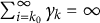 $\sum _{i=k_0}^\infty \gamma _k=\infty $
(Equation (9)), the right-hand side of Equation (A8) is
$\sum _{i=k_0}^\infty \gamma _k=\infty $
(Equation (9)), the right-hand side of Equation (A8) is
 $o(1)$
as
$o(1)$
as
 $k\to \infty $
.
$k\to \infty $
.
To bound
 $\mathrm {(II)}$
in Equation (A6), proceed similarly by noting that, for all
$\mathrm {(II)}$
in Equation (A6), proceed similarly by noting that, for all
 $k\ge k_0$
,
$k\ge k_0$
,
 $$ \begin{align} \begin{aligned} \mathrm{(II)}&=\left\|\sum_{j=1}^k \left\{\prod_{i=j+1}^k \left[I - \gamma_i \dot{\boldsymbol{L}}({\boldsymbol{\theta}}^*) \right]\right\} \gamma_j \mathbb{E}{\boldsymbol{h}}_j\right\|_\infty\\ &\le \sum_{j=1}^k\left\| \left\{\prod_{i=j+1}^k \left[\boldsymbol{I} - \gamma_i \dot{\boldsymbol{L}}({\boldsymbol{\theta}}^*) \right]\right\} \gamma_j \mathbb{E}{\boldsymbol{h}}_j\right\|_\infty \\ &\le \sum_{j=1}^k \left\| \left\{\prod_{i=j+1}^k \left[\boldsymbol{I} - \gamma_i \dot{\boldsymbol{L}}({\boldsymbol{\theta}}^*) \right]\right\} \right\|_\infty \gamma_j \|\mathbb{E}{\boldsymbol{h}}_j\|_1 \\ &\lesssim \sum_{j=k_0}^k \gamma_j\left\{\prod_{i=j+1}^k (1-\alpha\gamma_i)\right\} \|\mathbb{E}{\boldsymbol{h}}_j\|_1. \end{aligned} \end{align} $$
Now, we apply Lemma 1 of Sacks (Reference Sacks1958) to conclude that
 $$ \begin{align} \mathrm{(II)} \lesssim \|\mathbb{E}{\boldsymbol{h}}_\infty\|_1 \lesssim \left\|{\boldsymbol{\Sigma}}_{{\boldsymbol{\theta}}_\infty}({\boldsymbol{\theta}}^*)\right\|_2, \end{align} $$
in which
 ${\boldsymbol {\Sigma }}_{{\boldsymbol {\theta }}_\infty }({\boldsymbol {\theta }}^*) = \mathbb {E}[({\boldsymbol {\theta }}_\infty - {\boldsymbol {\theta }}^*) ({\boldsymbol {\theta }}_\infty - {\boldsymbol {\theta }}^*)^\top ]$
.
${\boldsymbol {\Sigma }}_{{\boldsymbol {\theta }}_\infty }({\boldsymbol {\theta }}^*) = \mathbb {E}[({\boldsymbol {\theta }}_\infty - {\boldsymbol {\theta }}^*) ({\boldsymbol {\theta }}_\infty - {\boldsymbol {\theta }}^*)^\top ]$
.
To justify the last inequality in Equation (A10), recall that the
 ${\boldsymbol {L}}^1$
norm of a vector is the sum of the absolute values of its components:
${\boldsymbol {L}}^1$
norm of a vector is the sum of the absolute values of its components:
 $$\begin{align*}\|\mathbb{E}{\boldsymbol{h}}_\infty\|_1 = \sum_{j=1}^p |\mathbb{E}[({\boldsymbol{f}}_\infty/2 + {\boldsymbol{\delta}}_\infty)_j]| \leq \frac{1}{2} \sum_{j=1}^p |\mathbb{E}[{\boldsymbol{H}}_j]| + \sum_{j=1}^p |\mathbb{E}[{\boldsymbol{\delta}}_j]|. \end{align*}$$
Thus, to bound
 $\|\mathbb {E}{\boldsymbol {h}}_\infty \|_1$
, it suffices to bound each component
$\|\mathbb {E}{\boldsymbol {h}}_\infty \|_1$
, it suffices to bound each component
 $|\mathbb {E}[{\boldsymbol {H}}_j]|$
and
$|\mathbb {E}[{\boldsymbol {H}}_j]|$
and
 $|\mathbb {E}[{\boldsymbol {\delta }}_j]|$
separately. We begin with the dominant term
$|\mathbb {E}[{\boldsymbol {\delta }}_j]|$
separately. We begin with the dominant term
 $\mathbb {E}[{\boldsymbol {H}}_j]$
. By Assumption A3,
$\mathbb {E}[{\boldsymbol {H}}_j]$
. By Assumption A3,
 ${\boldsymbol {H}}_j({\boldsymbol {\theta }}_\infty , {\boldsymbol {\theta }}^*) = ({\boldsymbol {\theta }}_\infty - {\boldsymbol {\theta }}^*)^\top \ddot {\boldsymbol {L}}_j({\boldsymbol {\theta }}^*)({{\boldsymbol {\theta }}_\infty } - {\boldsymbol {\theta }}^*)/2$
. Then,
${\boldsymbol {H}}_j({\boldsymbol {\theta }}_\infty , {\boldsymbol {\theta }}^*) = ({\boldsymbol {\theta }}_\infty - {\boldsymbol {\theta }}^*)^\top \ddot {\boldsymbol {L}}_j({\boldsymbol {\theta }}^*)({{\boldsymbol {\theta }}_\infty } - {\boldsymbol {\theta }}^*)/2$
. Then,
 $$ \begin{align*} |\mathbb{E}[{\boldsymbol{H}}_j({\boldsymbol{\theta}}_\infty, {\boldsymbol{\theta}}^*)]| &= \frac{1}{2} \left| \mathbb{E}[({\boldsymbol{\theta}}_\infty - {\boldsymbol{\theta}}^*)^\top \ddot{\boldsymbol{L}}_j({\boldsymbol{\theta}}^*)({\boldsymbol{\theta}}_\infty - {\boldsymbol{\theta}}^*)] \right| \\ &= \frac{1}{2} \left| \mathbb{E}[\mathrm{tr}(({\boldsymbol{\theta}}_\infty - {\boldsymbol{\theta}}^*)^\top \ddot{\boldsymbol{L}}_j({\boldsymbol{\theta}}^*)({\boldsymbol{\theta}}_\infty - {\boldsymbol{\theta}}^*))] \right| \\ &= \frac{1}{2} \left| \mathrm{tr}(\ddot{\boldsymbol{L}}_j({\boldsymbol{\theta}}^*) \mathbb{E}[({\boldsymbol{\theta}}_\infty - {\boldsymbol{\theta}}^*)({\boldsymbol{\theta}}_\infty - {\boldsymbol{\theta}}^*)^\top]) \right| \\ &= \frac{1}{2} \left| \mathrm{tr}(\ddot{\boldsymbol{L}}_j({\boldsymbol{\theta}}^*) {\boldsymbol{\Sigma}}_{{\boldsymbol{\theta}}_\infty}({\boldsymbol{\theta}}^*)) \right| \\ &\leq \frac{1}{2} \|\ddot{\boldsymbol{L}}_j({\boldsymbol{\theta}}^*)\|_* \|{\boldsymbol{\Sigma}}_{{\boldsymbol{\theta}}_\infty}({\boldsymbol{\theta}}^*)\|_2, \end{align*} $$
where
 $\|\cdot \|_*$
denotes the nuclear (trace) norm and the inequality follows from Hölder’s inequality for Schatten norms. Since
$\|\cdot \|_*$
denotes the nuclear (trace) norm and the inequality follows from Hölder’s inequality for Schatten norms. Since
 $\ddot {\boldsymbol {L}}_j({\boldsymbol {\theta }}^*)$
is a fixed matrix (independent of n), its nuclear norm is bounded.
$\ddot {\boldsymbol {L}}_j({\boldsymbol {\theta }}^*)$
is a fixed matrix (independent of n), its nuclear norm is bounded.
As for the remainder term
 $\mathbb {E}[{\boldsymbol {\delta }}_j]$
, by Assumption A3, we have
$\mathbb {E}[{\boldsymbol {\delta }}_j]$
, by Assumption A3, we have
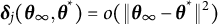 ${\boldsymbol {\delta }}_j({\boldsymbol {\theta }}_\infty , {\boldsymbol {\theta }}^*) = o(\|{\boldsymbol {\theta }}_\infty - {\boldsymbol {\theta }}^*\|^2)$
, which implies that
${\boldsymbol {\delta }}_j({\boldsymbol {\theta }}_\infty , {\boldsymbol {\theta }}^*) = o(\|{\boldsymbol {\theta }}_\infty - {\boldsymbol {\theta }}^*\|^2)$
, which implies that
 $|\mathbb {E}[{\boldsymbol {\delta }}_j]|$
is of higher order and can be bounded by a constant multiple of
$|\mathbb {E}[{\boldsymbol {\delta }}_j]|$
is of higher order and can be bounded by a constant multiple of
 $\|{\boldsymbol {\Sigma }}_{{\boldsymbol {\theta }}_\infty }({\boldsymbol {\theta }}^*)\|_2$
using similar arguments. Combining the bounds for all components
$\|{\boldsymbol {\Sigma }}_{{\boldsymbol {\theta }}_\infty }({\boldsymbol {\theta }}^*)\|_2$
using similar arguments. Combining the bounds for all components
 $j = 1, \dots , p$
yields the desired inequality.
$j = 1, \dots , p$
yields the desired inequality.
To further analyze the order of
 $\|{\boldsymbol {\Sigma }}_{{\boldsymbol {\theta }}_\infty }({\boldsymbol {\theta }}^*)\|_2$
, consider the one-term expansion
$\|{\boldsymbol {\Sigma }}_{{\boldsymbol {\theta }}_\infty }({\boldsymbol {\theta }}^*)\|_2$
, consider the one-term expansion
 $$ \begin{align} \boldsymbol{L}({\boldsymbol{\theta}}_\infty) = \boldsymbol{L}({\boldsymbol{\theta}}^*) + \dot{\boldsymbol{L}}(\tilde{\boldsymbol{\theta}})({\boldsymbol{\theta}}_\infty- {\boldsymbol{\theta}}^*), \end{align} $$
in which
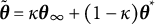 $\tilde {\boldsymbol {\theta }} = \kappa {\boldsymbol {\theta }}_\infty + (1 - \kappa ){\boldsymbol {\theta }}^*$
for some
$\tilde {\boldsymbol {\theta }} = \kappa {\boldsymbol {\theta }}_\infty + (1 - \kappa ){\boldsymbol {\theta }}^*$
for some
 $0\le \kappa \le 1$
. Recall that
$0\le \kappa \le 1$
. Recall that
 $\boldsymbol {L}({\boldsymbol {\theta }}_\infty ) = \hat {\boldsymbol {\theta }}$
(see Equation (5)) and that
$\boldsymbol {L}({\boldsymbol {\theta }}_\infty ) = \hat {\boldsymbol {\theta }}$
(see Equation (5)) and that
 $\boldsymbol {L}({\boldsymbol {\theta }}^*) = \hat {\boldsymbol {\theta }}$
. Therefore,
$\boldsymbol {L}({\boldsymbol {\theta }}^*) = \hat {\boldsymbol {\theta }}$
. Therefore,
 $$ \begin{align} {\boldsymbol{\Sigma}}_{\hat{\boldsymbol{\theta}}}({\boldsymbol{\theta}}^*) = \mathbb{E}[(\hat{\boldsymbol{\theta}} - \mathbb{E}\hat{\boldsymbol{\theta}})(\hat{\boldsymbol{\theta}} - \mathbb{E}\hat{\boldsymbol{\theta}})^\top] = \mathbb{E}[\dot{\boldsymbol{L}}(\tilde{\boldsymbol{\theta}})({\boldsymbol{\theta}}_\infty - {\boldsymbol{\theta}}^*)({\boldsymbol{\theta}}_\infty - {\boldsymbol{\theta}}^*)^\top\dot{\boldsymbol{L}}(\tilde{\boldsymbol{\theta}})^\top]. \end{align} $$
By Assumptions A2 and A4, we have
 $$ \begin{align} \|{\boldsymbol{\Sigma}}_{{\boldsymbol{\theta}}_\infty}({\boldsymbol{\theta}}^*)\|_2 = \left\|\mathbb{E}[({\boldsymbol{\theta}}_\infty - {\boldsymbol{\theta}}^*)({\boldsymbol{\theta}}_\infty - {\boldsymbol{\theta}}^*)^\top]\right\|_2\lesssim\|{\boldsymbol{\Sigma}}_{\hat{\boldsymbol{\theta}}}({\boldsymbol{\theta}}^*)\|_2 = O(n^{-1}). \end{align} $$
Combining Equations (A6), (A8), (A10), and (A13) concludes the proof of the theorem.
A3 Standard error estimation
We next introduce a practical strategy to estimate the SEs of the bias-corrected estimator
 ${\boldsymbol {\theta }}_\infty $
. More specifically, the theorem implies the consistency of
${\boldsymbol {\theta }}_\infty $
. More specifically, the theorem implies the consistency of
 ${\boldsymbol {\theta }}_\infty $
; therefore, by Equation (A11) and the continuous mapping theorem, we have
${\boldsymbol {\theta }}_\infty $
; therefore, by Equation (A11) and the continuous mapping theorem, we have
 $$ \begin{align} {\boldsymbol{\theta}}_\infty - {\boldsymbol{\theta}}^* = \dot{\boldsymbol{L}}({\boldsymbol{\theta}}^*)^{-1}(\hat{\boldsymbol{\theta}} - \mathbb{E}\hat{\boldsymbol{\theta}}) + o_p(1). \end{align} $$
Equation (A14) suggests that
 $$ \begin{align} {\boldsymbol{\Sigma}}_{{\boldsymbol{\theta}}_\infty}({\boldsymbol{\theta}}^*) \approx \dot{\boldsymbol{L}}({\boldsymbol{\theta}}^*)^{-1}{\boldsymbol{\Sigma}}_{\hat{\boldsymbol{\theta}}}({\boldsymbol{\theta}}^*) \dot{\boldsymbol{L}}({\boldsymbol{\theta}}^*)^{-\top}. \end{align} $$
In practice, Equation (A15) cannot be directly evaluated due to the unknown
 ${\boldsymbol {\theta }}^*$
. However, valid SEs can still be obtained using a consistent estimator of
${\boldsymbol {\theta }}^*$
. However, valid SEs can still be obtained using a consistent estimator of
 ${\boldsymbol {\Sigma }}_{{\boldsymbol {\theta }}_\infty }({\boldsymbol {\theta }}^*)$
. For instance, we can consistently estimate
${\boldsymbol {\Sigma }}_{{\boldsymbol {\theta }}_\infty }({\boldsymbol {\theta }}^*)$
. For instance, we can consistently estimate
 $\dot {\boldsymbol {L}}(\boldsymbol {\theta }^*)$
by
$\dot {\boldsymbol {L}}(\boldsymbol {\theta }^*)$
by
 $\dot {\boldsymbol {L}}({\boldsymbol {\theta }}_\infty )$
and
$\dot {\boldsymbol {L}}({\boldsymbol {\theta }}_\infty )$
and
 ${\boldsymbol {\Sigma }}_{\hat {\boldsymbol {\theta }}}(\boldsymbol {\theta }^*)$
by
${\boldsymbol {\Sigma }}_{\hat {\boldsymbol {\theta }}}(\boldsymbol {\theta }^*)$
by
 ${\boldsymbol {\Sigma }}_{\hat {\boldsymbol {\theta }}}({\boldsymbol {\theta }}_\infty )$
. Monte Carlo (MC) estimates of
${\boldsymbol {\Sigma }}_{\hat {\boldsymbol {\theta }}}({\boldsymbol {\theta }}_\infty )$
. Monte Carlo (MC) estimates of
 $\dot {{\boldsymbol {L}}}$
and
$\dot {{\boldsymbol {L}}}$
and
 ${\boldsymbol {\Sigma }}_{\hat {\boldsymbol {\theta }}}$
can be substituted if closed-form expressions do not exist. For the simulation and empirical example reported in the current study, we approximate Equation (A15) by
${\boldsymbol {\Sigma }}_{\hat {\boldsymbol {\theta }}}$
can be substituted if closed-form expressions do not exist. For the simulation and empirical example reported in the current study, we approximate Equation (A15) by
 $$ \begin{align} \widehat{\boldsymbol{\Sigma}}_{{\boldsymbol{\theta}}_\infty}({\boldsymbol{\theta}}^*) = \left[ \widehat{\dot{\boldsymbol{L}}}\left( {\overline{\boldsymbol{\theta}}}_{K} \right) \right]^{-1} \widehat{\boldsymbol{\Sigma}}_{\hat{\boldsymbol{\theta}}}({\overline{\boldsymbol{\theta}}}_{K}) \left[ {\widehat{\dot{\boldsymbol{L}}}\left( {\overline{\boldsymbol{\theta}}}_{K} \right)} \right]^{-\top}, \end{align} $$
in which
 ${\overline {\boldsymbol {\theta }}}_{K}$
is computed by Equation (11),
${\overline {\boldsymbol {\theta }}}_{K}$
is computed by Equation (11),
 $\widehat {\boldsymbol {\Sigma }}_{\hat {\boldsymbol {\theta }}}({\overline {\boldsymbol {\theta }}}_{K})$
is an MC estimate of
$\widehat {\boldsymbol {\Sigma }}_{\hat {\boldsymbol {\theta }}}({\overline {\boldsymbol {\theta }}}_{K})$
is an MC estimate of
 ${\boldsymbol {\Sigma }}_{\hat {\boldsymbol {\theta }}}({\boldsymbol {\theta }}^*)$
using
${\boldsymbol {\Sigma }}_{\hat {\boldsymbol {\theta }}}({\boldsymbol {\theta }}^*)$
using
 $\overline {\boldsymbol {\theta }}_K$
as the data-generating parameters, and the Jacobian matrix
$\overline {\boldsymbol {\theta }}_K$
as the data-generating parameters, and the Jacobian matrix
 $\widehat {\dot {\boldsymbol {L}}}\left ( {\overline {\boldsymbol {\theta }}}_{K} \right )$
is estimated via numerical differentiation.
$\widehat {\dot {\boldsymbol {L}}}\left ( {\overline {\boldsymbol {\theta }}}_{K} \right )$
is estimated via numerical differentiation.


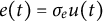
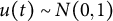


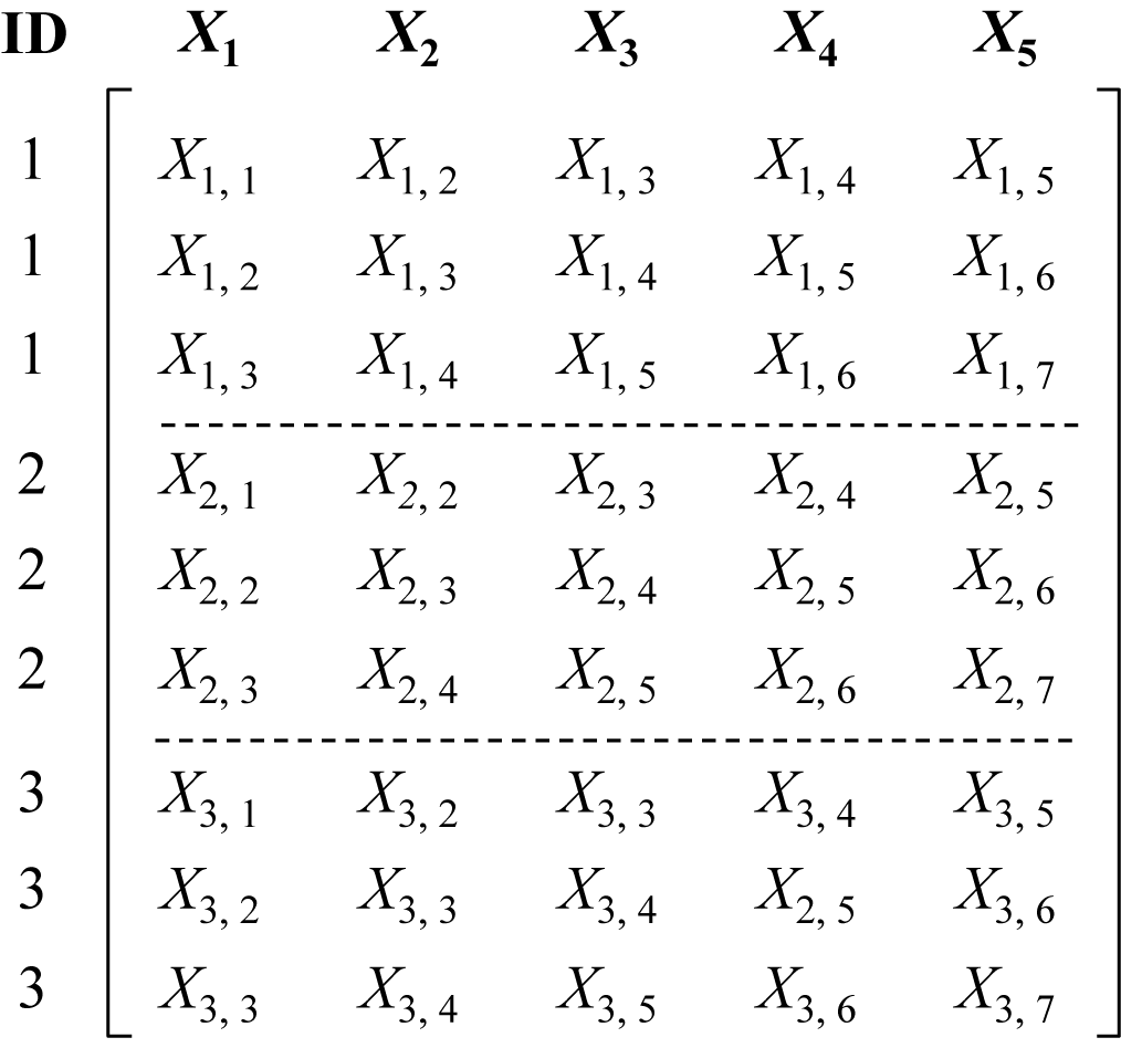


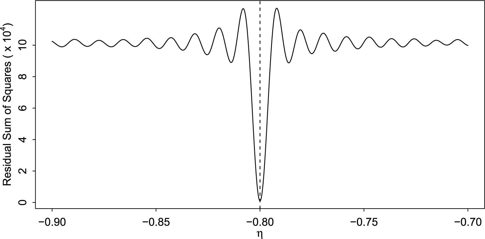


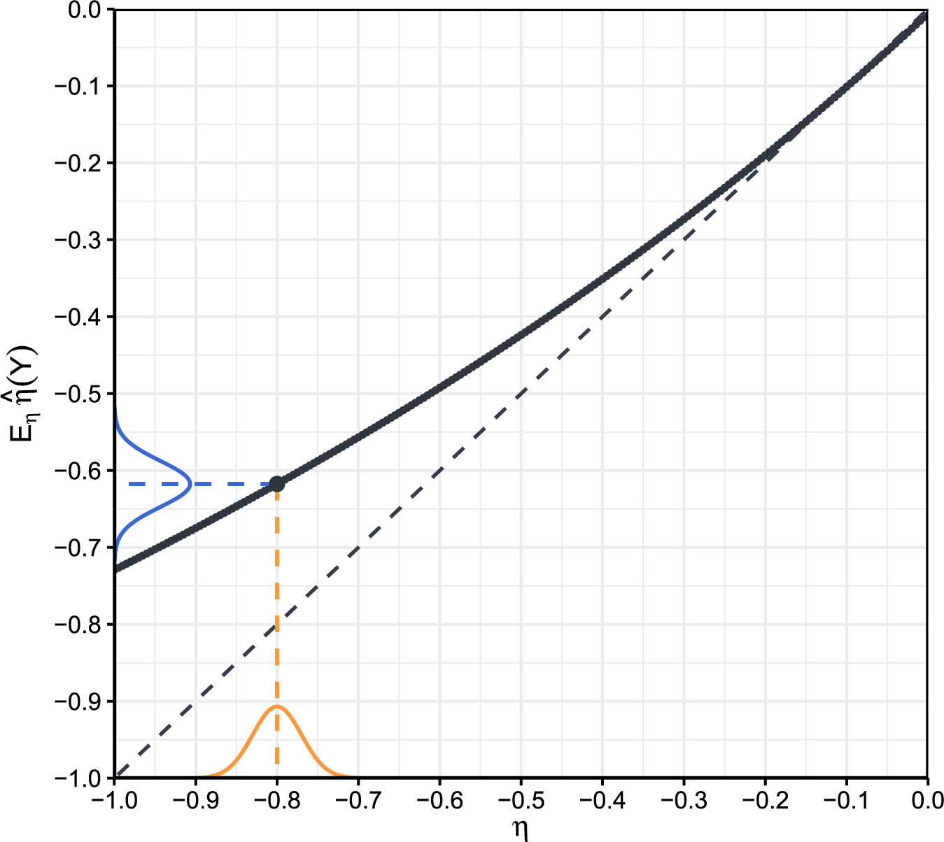


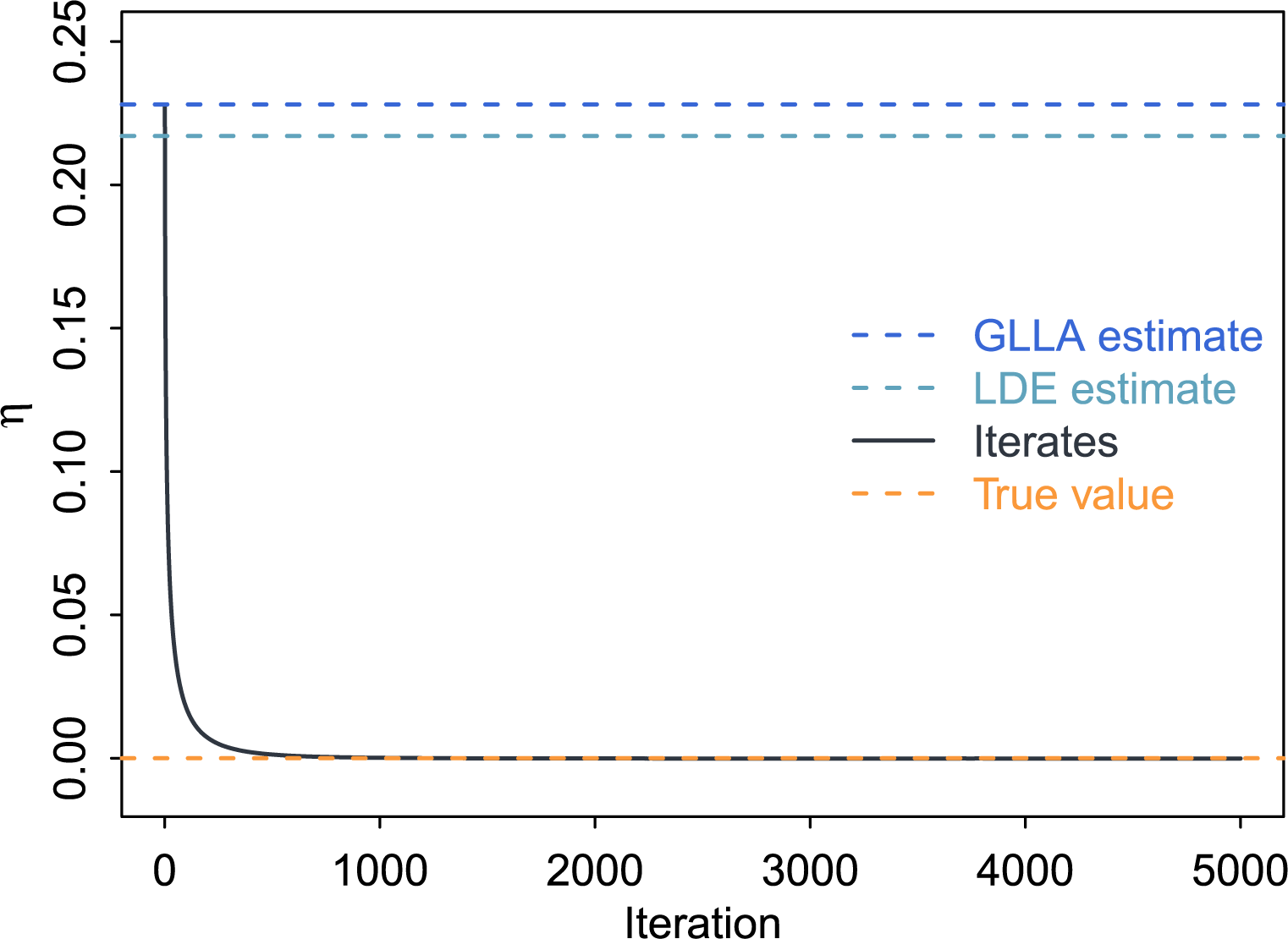


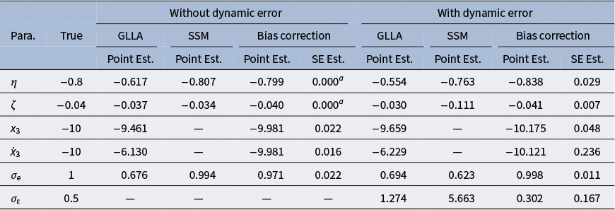
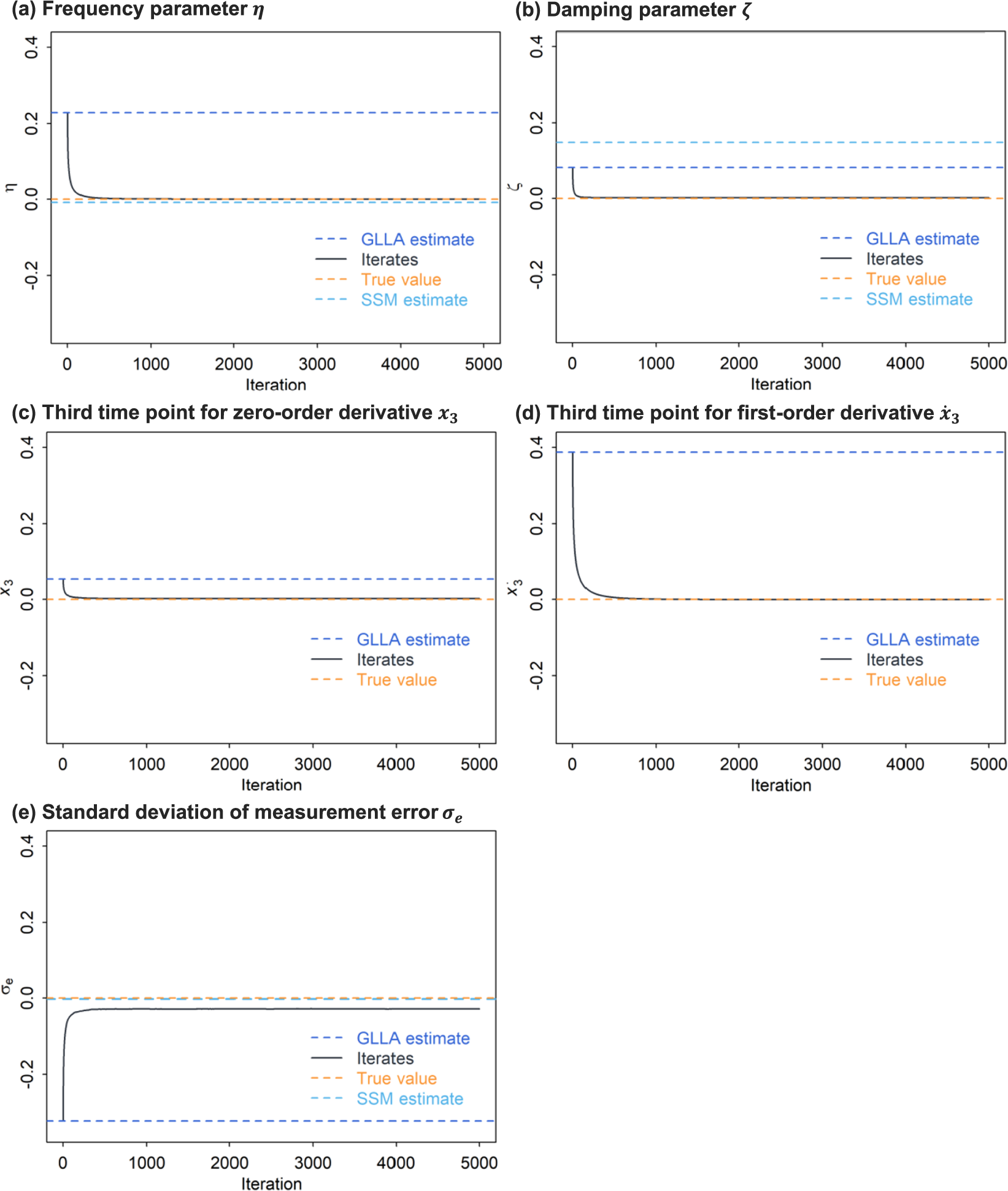
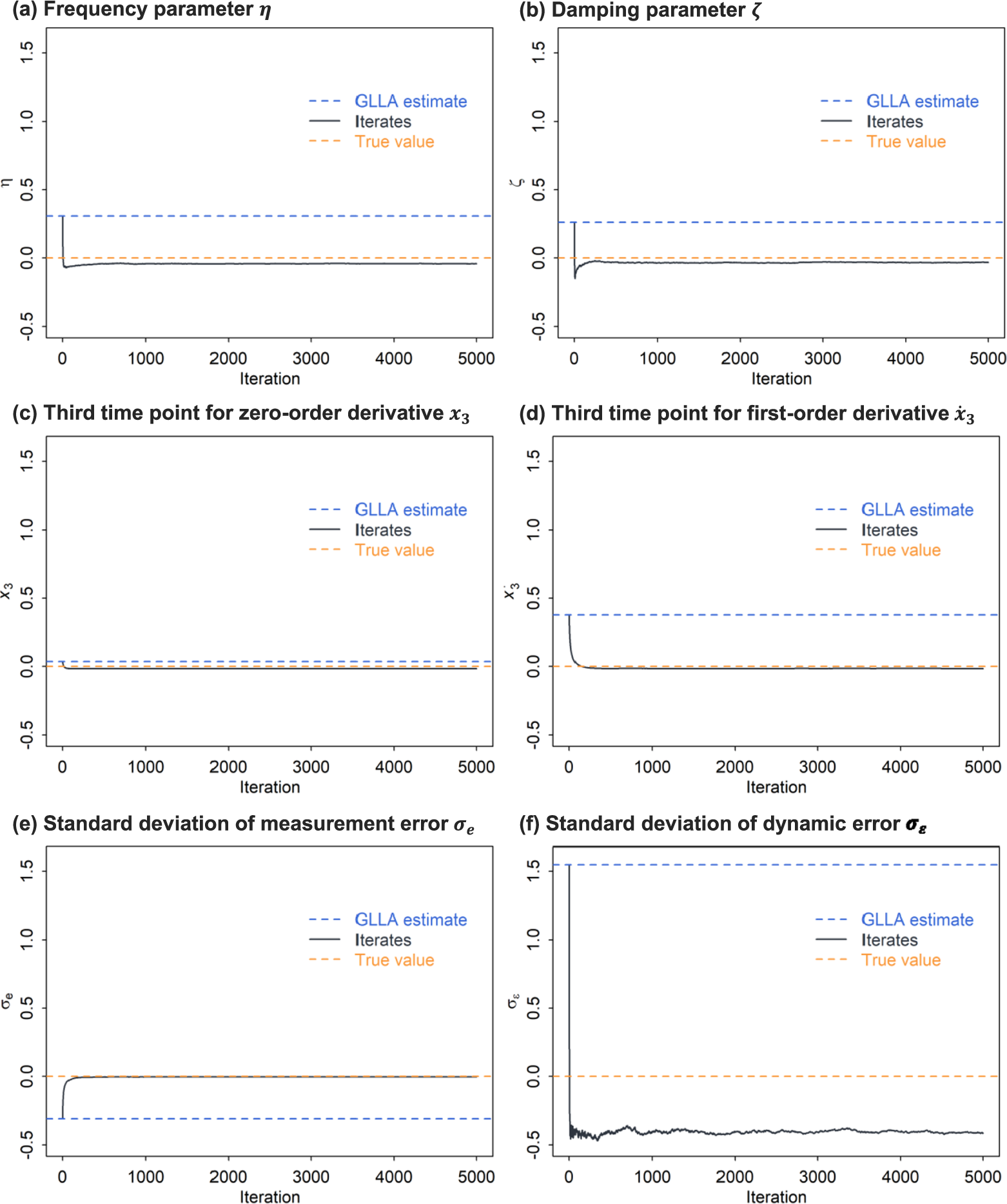

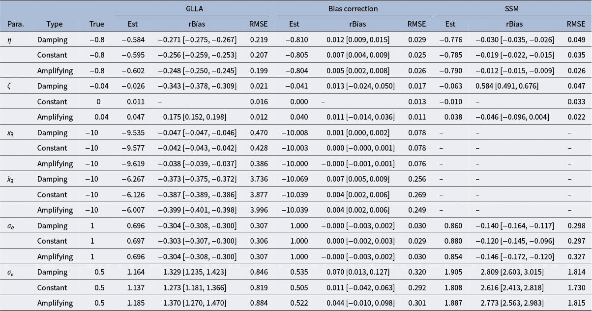
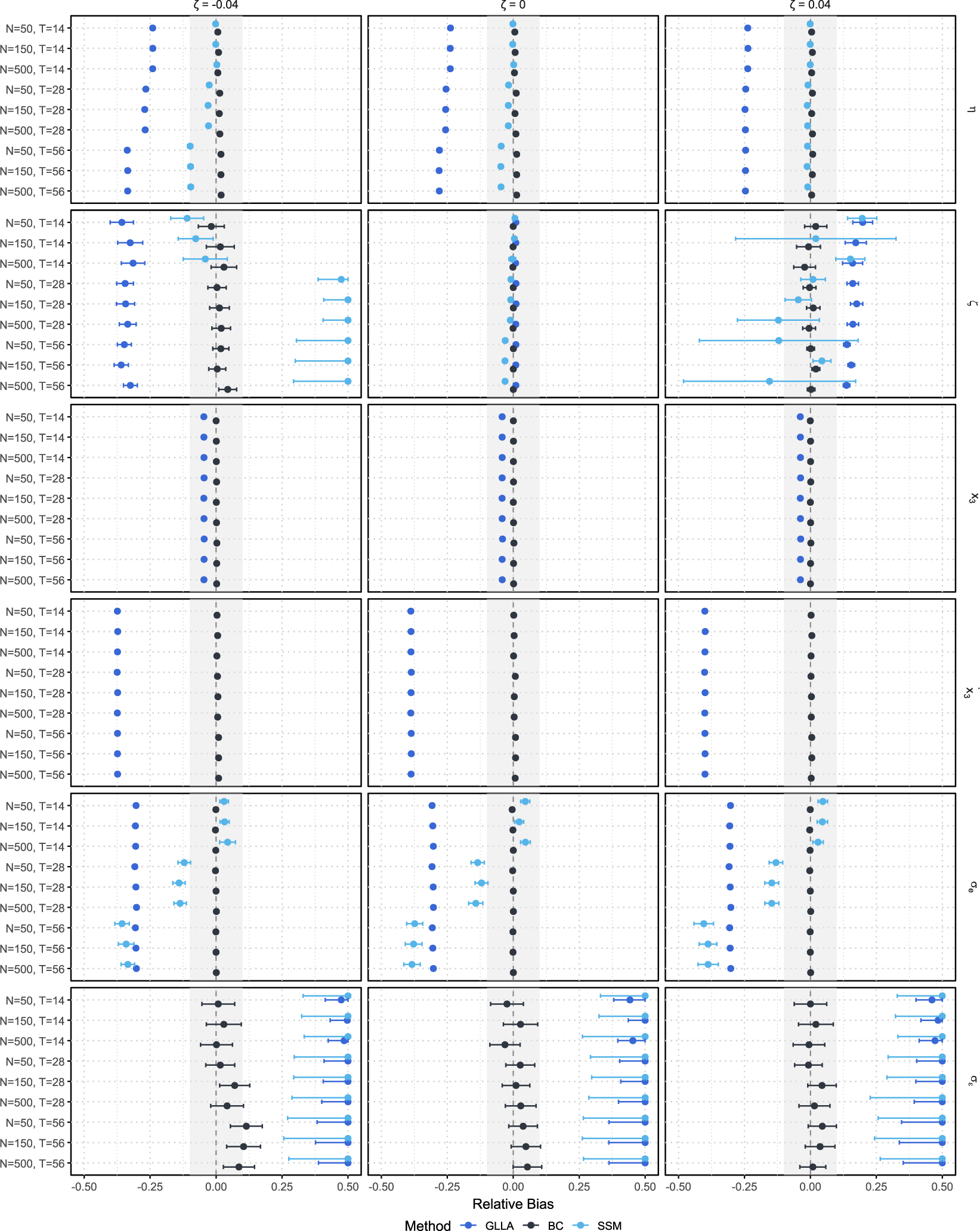


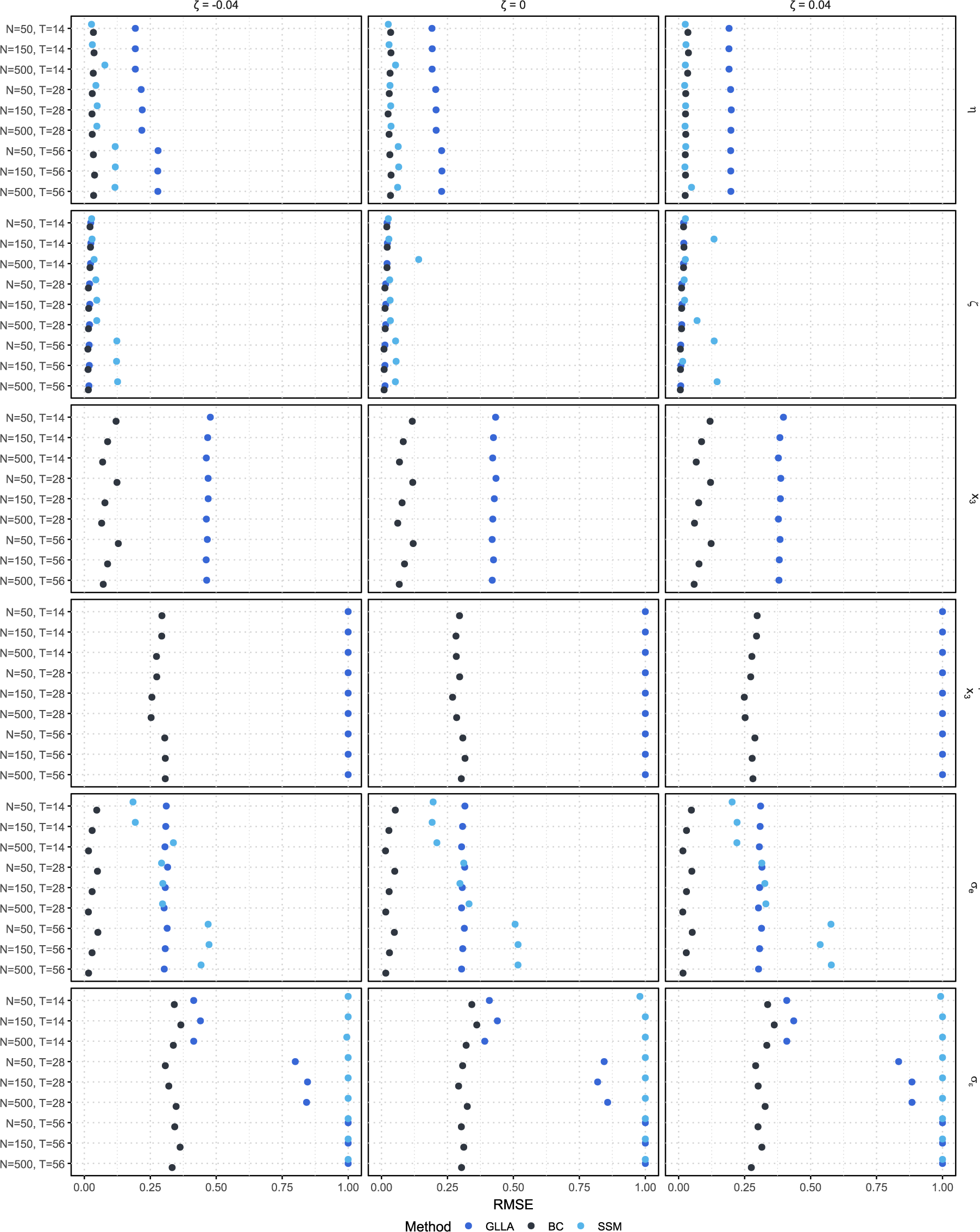
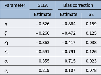
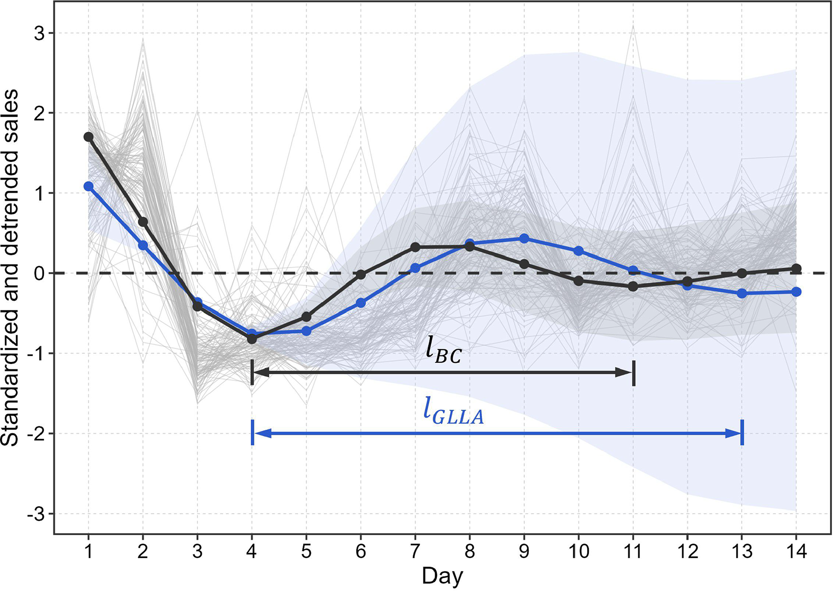


 Open access