


1. INTRODUCTION
Sea-ice thickness (SIT) is one of the essential climate variables that critically contributes to the characterization of Earth's climate (WMO, 2018). SIT is used in estimating the sea-ice volume, high-latitude heat-budget, ship navigation, global ocean circulation of the Earth system (Vinnikov and others, Reference Vinnikov1999; Maksym, Reference Maksym2019) and SIT data assimilation in regional ice prediction and global climate models (Chen and others, Reference Chen, Liu, Song, Yang and Xu2017). Accurate knowledge of SIT is sparse and insufficient at the desired temporal (daily) and spatial (<25 km) scales (Lindsay and Schweiger, Reference Lindsay and Schweiger2015). The volume of sea ice is inaccurately estimated due to uncertainty in SIT and its distribution caused by non-uniform, anisotropic and heterogeneous nature of the surface and bottom of sea ice. Many regional and global climate models use the thermodynamic model of sea-ice growth. The ice growth model has not been verified yet. Thus, the problem of remote-sensing retrieval of SIT and its adequate use in various regional ice prediction and global climate models is still a topic of active research.
There are a number of means by which information on SIT can be obtained. These can be categorized into invasive (in situ on-ice measurements) and non-invasive (remote-sensing) methods. Remote-sensing methods include passive microwave radiometry (Kaleschke and others, Reference Kaleschke, Tian-Kunze, Maaß, Mäkynen and Drusch2012; Nakata and others, Reference Nakata, Ohshima and Nihashi2018), helicopter-based electromagnetic (EM) induction system (Haas and others, Reference Haas, Lobach, Hendricks, Rabenstein and Pfaffling2009; Hunkeler and others, Reference Hunkeler2016), ice freeboard measurements from Cryosat-2 radar altimeter (Laxon and others, Reference Laxon2013; Yi and others, Reference Yi2019), ICESat laser altimeter (Kwok and Rothrock, Reference Kwok and Rothrock2009; Nihashi and others, Reference Nihashi2018), upward-looking sonar (ULS) (Hudson, Reference Hudson1990; Kwok, Reference Kwok2018), Global Navigation Satellite Systems-Reflectometry (GNSS-R) (Li and others, Reference Li2017) and Ground-Penetrating Radar (GPR) (Matsumoto and others, Reference Matsumoto, Yoshimura, Naoki, Cho and Wakabayashi2018). While other remote-sensing methods are either swath-limited (e.g. altimeters), or provide sparse spatial coverage (e.g. ULS), passive microwave radiometry offers continuous, all-weather, Arctic-wide coverage of SIT at different spatial resolutions. However, passive microwave radiometry for SIT retrieval is limited to the cold and dry winter season typically from mid-October to mid-April in the Arctic. During summer, the increasing liquid water content at the snow–air and snow–ice interface results in dramatic change of brightness temperature (TB) by the wet surface. Relatively high penetration depth at L-band and high TB contrast between ice and water at this frequency (~100 K at 1.4135 GHz) allow the assessment of the potential of retrieving SIT (Huntemann and others, Reference Huntemann2014).
Kaleschke and others (Reference Kaleschke, Tian-Kunze, Maaß, Mäkynen and Drusch2012) proposed an algorithm for estimating SIT up to 0.55 m using the TB from Soil Moisture and Ocean Salinity (SMOS) mission. The estimation of SIT from passive microwave TB involves a number of approximations and uncertainties, which also depend on several factors including the type of emissivity model of sea ice. Kaleschke and others (Reference Kaleschke, Tian-Kunze, Maaß, Mäkynen and Drusch2012) assumed ice temperature and ice salinity as constants, which turn out to be a major drawback of this algorithm (Tian-Kunze and others, Reference Tian-Kunze2014). Tian-Kunze and others (Reference Tian-Kunze2014) (Algorithm II) overcame this issue by considering the profiles of ice temperature and salinity varying with depth within the ice column. Algorithm II enables SIT estimates up to ~1.5 m. Algorithm II also has several shortcomings due to the fact that SIT retrieval is dependent on many factors such as sea-ice concentration (SIC), ice thickness distribution within the grid size, ice salinity, ice temperature and many others. The major drawback of Algorithm II lies in its inability to differentiate low SIC from thin SIT areas as both have similar TB. It retrieves thin SIT values in areas of the Arctic Ocean where SIC is <100%. Huntemann and others (Reference Huntemann2014) presented another approach to retrieve SIT, which used polarization difference (PD) (at 40–50° incidence angle) instead of TB and predicted thin SIT based on a regression equation derived from TOPAZ (Sakov and others, Reference Sakov2012) and the Cumulative Freezing Degree Days model. This approach also derives SIT in areas with SIC much <100%.
SMOS, a mission to measure SMOS and based on the Microwave Imaging Radiometer by Aperture Synthesis (MIRAS), is one of the Earth Explorer Opportunity missions from European Space Agency (ESA). It was launched on 2 November 2009 from Plesetsk Cosmodrome in Russia on Rockot launch vehicle. It offers TB of the Earth's surface in dual- and full-polarization, at different incidence angles (0–65°) and spatial resolutions from 35 km at the center of the field of view (FOV) to 50 km at the edge of the snapshot, with a wide swath of 1200 km. The principal objective of the SMOS mission is to provide maps of SMOS; however, as the knowledge from SMOS grew over the years, the data turned out to be exceedingly useful for cryosphere studies. The SMOS TB were explored for relation with the SIC (Gabarro and others, Reference Gabarro, Turiel, Elosegui, Pla-Resina and Portabella2017), thin SIT (Kaleschke and others, Reference Kaleschke, Maaß, Haas, Heygster and Tonboe2010, Reference Kaleschke, Tian-Kunze, Maaß, Mäkynen and Drusch2012; Huntemann and others, Reference Huntemann2014; Tian-Kunze and others, Reference Tian-Kunze2014), snow thickness (Maaß and others, Reference Maaß, Kaleschke, Tian-Kunze and Drusch2013; Zhou and others, Reference Zhou, Xu, Liu and Wang2018), soil moisture (Kerr and others, Reference Kerr2012; Khodayar and others, Reference Khodayar, Coll and Lopez-Baeza2019), sea surface salinity (SSS) (Font and others, Reference Font2010; Olmedo and others, Reference Olmedo, Taupier-Letage, Turiel and Alvera-Azcárate2018) and in many other earth applications. The ‘SMOSIce project’ (L-band Radiometry for Sea-Ice Applications Study) was conducted during 2010–13 to explore the potential of retrieving SIT from SMOS L-band TB (Heygster and others, Reference Heygster2009; Kaleschke and others, Reference Kaleschke2013).
In this paper, a new method is proposed for retrieving thin SIT by establishing a direct empirical relationship between SIT acquired through various ‘airborne sea-ice thickness’ (hereinafter: ASIT) campaigns throughout the Arctic during 2011–15 and SMOS PD at 50° incidence angle. This is the first empirical study that exclusively uses only ASIT data to train the algorithm. The latest version of SMOS Level 1B TB data in the Arctic has been used at 25 km SMOS grid during cold and dry months (October–April). Based on this algorithm, an operational thin SIT product of the Arctic has been generated for public to be available for download from the Barcelona Expert Center (BEC) website http://bec.icm.csic.es/. The paper is organized as follows: the data used are described in Section 2; the empirical approach methodology is presented in Section 3; results and validation are in Section 4; discussions on comparison with other SIT products in Section 5; and conclusions in the final Section 6.
2. DATA
2.1 SMOS data used
ESA provides SMOS TB science data in Level 1 and Level 2 products. This includes the complete Level 1B/1C and Level 2 soil moisture/ocean salinity data. ESA Level 1C is provided in Icosahedral Snyder Equal Area (ISEA) 4H9 grid. This is a hexagonal grid having a constant area of each cell and a non-uniform distance ~15 km between the centers of two adjacent cells. The instrumental resolution of SMOS for a single snapshot varies from 35 to 50 km depending on the pixel position in the reconstructed image. As shown by Talone and others (Reference Talone, Portabella, Martínez and González-Gambau2015), the maximum independence among measurements of the same snapshot, with a minimum loss of information, is attached to using spatial resolutions ~25 km. The use of smaller resolution grids with the SMOS measures would result in interpolation and therefore inaccuracies in the retrieval of geophysical variables. Therefore, the raw SMOS Level 1B (L1B) product has been used instead of traditional Level 1C to be able to obtain TB and retrieve SIT at this spatial resolution. A 25 km wide Equal-Area Scalable Earth North Azimuthal (NL EASE) grid is an appropriate grid for polar projections and fits well with the reconstruction image performed from Level 1B product.
The radiometric accuracy of individual TB observations is the lowest (~2 K) at antenna boresight, and it increases for lower and higher incidence angles (Kaleschke and others, Reference Kaleschke2013; Gabarro and others, Reference Gabarro, Turiel, Elosegui, Pla-Resina and Portabella2017). In radiometric measurements from space, as microwave radiation from Earth propagates through the ionosphere, the EM field components are rotated by an angle, called Faraday rotation, which depends on the total electron content present in the ionosphere, the frequency and the geomagnetic field (Corbella and others, Reference Corbella, Wu, Torres, Duffo and Martín-Neira2015). Faraday rotation is not negligible at SMOS operating frequency (1.4135 Hz) and must be corrected to have TB expressed in the Earth reference frame. This is not the only correction necessary that is taken into consideration; the correction has also been made in the TB associated with physical processes such as atmospheric self-emission and atmospheric attenuation of the upwelling brightness (Zine and others, Reference Zine2008). The L-band galactic emission reflected by sea or ice surface should be also taken into consideration in order to obtain the true radiation emitted by the ice. As the Earth makes one complete revolution of the Sun, it crosses the galactic plane twice; thus, two peaks of galactic noise are observed. The magnitude of galactic noise is dependent on the latitude (De Lannoy and others, Reference De Lannoy2015). Nevertheless, the galactic noise has not been corrected as it is considered insignificant for the Polar Regions.
Once measured TB values are converted from the original antenna reference frame to the Earth reference frame and all relevant external sources are corrected, a filter of outliers is applied to them. For each Earth surface point, the obtained TB values depend on the incidence angle at which they have been measured. TB has a smooth dependence on the incidence angle (Zine and others, Reference Zine2008). Therefore, it is assumed that the relationship among TB for three consecutive values of incidence angle can be considered as linear. Consequently, the TB values that deviated by more than three times the radiometric accuracy as compared with TB values of the two closer incidence angles were removed.
The hexagonal sampling in the Fourier domain results in aliasing, i.e. earth replicas or overlap with earth image in the reconstructed TB (Camps and others, Reference Camps, Vall-llossera, Duffo, Torres and Corbella2005). The alias-free TB data are used for SIT retrieval in this paper, and the direct and reflected Sun (Sun glint) and its tails from the TB values have also been corrected.
SMOS data pertaining to the ascending and descending passes were taken for three consecutive days and the TB values were averaged. The optimal incidence angle at 50° has been chosen for SIT retrieval after performing the sensitivity analysis of different incidence angles with PD values (Gabarro and others, Reference Gabarro, Turiel, Elosegui, Pla-Resina and Portabella2017). Though the Radio Frequency Interference (RFI) in SMOS TB observations has reduced since 2009, a threshold of 300 K is put on the TB beyond which the values are discarded. The minimum threshold value of TB at 50° incidence angle for SIT retrieval analysis is taken as 115 K.
2.2 Airborne SIT data
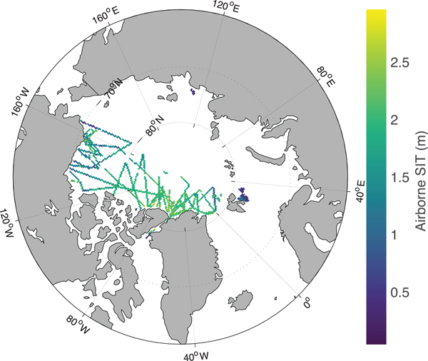
A large amount of ASIT data have been used in this paper from various field campaigns in the Arctic conducted by different countries during the 2011–15 period (Fig. 1, Table 1). Unfortunately, very few campaigns have acquired ASIT data (both thin and thick) in the Arctic during 2011–2015. The only ASIT data available for use from 2011 to 2015 are listed in Table 1. Airborne thin SIT data are difficult to acquire under harsh Arctic conditions and such campaigns are rare. The months of March–April are normally cold and dry in the Arctic with zero probability of liquid water content in the ice column or at any ice interface thus facilitating the penetration of microwaves. SIT data sources are: Seasonal Ice Zone Observational Network (SIZONet) in Chukchi Sea (NSF, 2009); National Aeronautics and Space Administration (NASA) Operation IceBridge (OIB) Airborne Topographic Mapper (ATM) in the central Arctic Ocean, Beaufort Sea and Upper Baffin Bay (Kurtz and others, Reference Kurtz, Studinger, Harbeck, Onana and Yi2015); EM bird (EMB) dataset for exclusive thin SIT validation from ESA SMOSIce (Barents Sea) and Alfred Wegener Institute (AWI) campaigns (Haas and others, Reference Haas, Lobach, Hendricks, Rabenstein and Pfaffling2009; Hendricks and others, Reference Hendricks2014; Kaleschke and others, Reference Kaleschke2016); TD XX campaign in Laptev Sea (Krumpen, Reference Krumpen2017); and N-ICE Campaign (King and others, Reference King, Gerland, Spreen and Bratrein2016) (Table 1). All of the above SIT data are available from respective websites provided under references. Almost all ASIT data used in this study are acquired using the EM induction system except the OIB data, which use freeboard method from laser altimetry (ATM) to retrieve the SIT. The ATM lidar is a conically scanning, full-waveform system that transmits 532 nm wavelength 6 ns pulses with a 3 or 5 kHz repetition rate (Kurtz and others, Reference Kurtz2013; Brunt and others, Reference Brunt2017). The listed averaged accuracies of SIT from EM induction and OIB data are 0.10 m (Haas and others, Reference Haas, Lobach, Hendricks, Rabenstein and Pfaffling2009) and 0.40 m (Farrell and others, Reference Farrell2012), respectively.
Geographic locations of ASIT (only 0–3 m) data from various EMB and OIB campaigns during 2011–15.
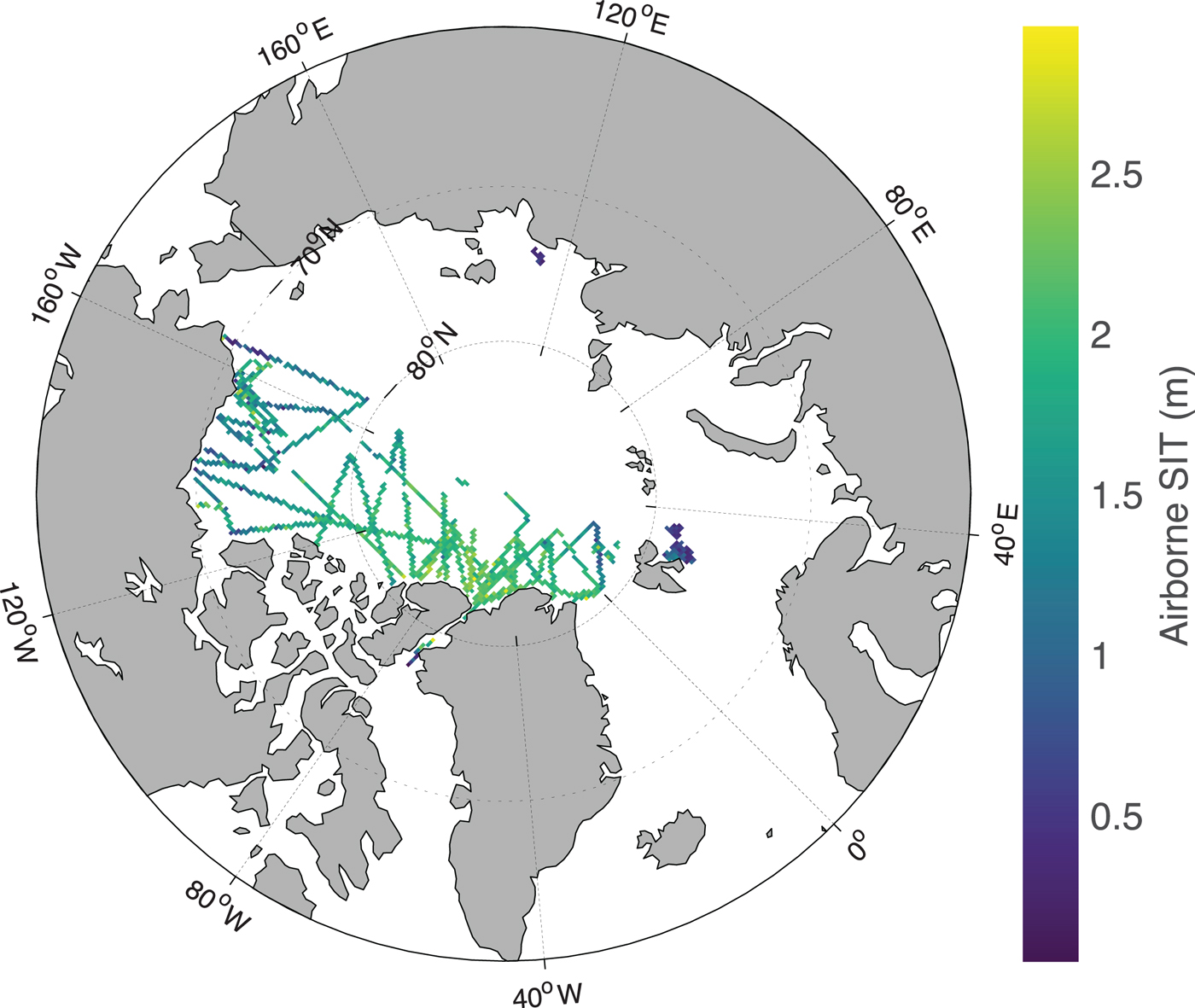
The ASIT data used in the paper from different Arctic field campaigns conducted during 2011–15. The flight tracks are shown in Figure 1

The total number of original, unaveraged, independent ASIT points is 1 388 511 and the total number of 25 km SMOS collocated grids is 1988. The number of SMOS grids collocated with the EMB data alone is 340. The airborne EMB data are divided into two groups, one for training the algorithm (consisting of 220 EMB and all OIB SIT values) and the other for validating the method (120 EMB SIT values). The data used exclusively for validation (and therefore excluded from algorithm training) are from the ESA SMOSIce and the AWI campaigns. No other airborne thin SIT data source exists during 2011–15 suitable for validation analysis at 25 km grid. The thin SIT data for these campaigns correspond to the following dates: 22 March 2014, and 8, 9, 11 and 22 April 2015, which upon collocating with SMOS at 25 km grid correspond to 120 independent grids (shown in Table 2). As the focus in this paper is only on thin sea ice, a significant difference in the computed SIT (hereinafter: BEC SIT) statistics is not expected from freeze-up (November) to winter-maximum (March–April). The seasons do not matter much, provided that surface conditions are cold (~−10 °C or below) and dry (zero liquid water content).
Exclusive thin SIT validation data from ESA SMOSIce and AWI EMB campaigns (Hendricks and others, Reference Hendricks2014). The SMOS collocated airborne data correspond to 120 independent grids

2.3 SIC data
The coincident operational SIC products (OSI-401-b) from European Organization for the Exploitation of Meteorological Satellites (EUMETSAT) Ocean and Sea Ice Satellite Application Facility (OSI SAF) have been used for the period of 2011–15. The OSI SAF generates SIC products using atmospherically corrected TB from Special Sensor Microwave Imager/Sounder (SSMI/S) and combining state-of-the-art algorithms (Tonboe and others, Reference Tonboe, Lavelle, Pfeiffer and Howe2017). The daily global SIC data for 2011–15 were downloaded as Network Common Data Form (NetCDF or .nc file) files on 10 km polar stereographic projection grid. The OSI SAF SIC data are re-gridded to 25 km to collocate with the BEC SIT product using linear 2D-interpolation. The SIC products are available at ftp://osisaf.met.no/../archive/ice/conc/.
2.4 Other SIT products
Two other SIT products have been used for inter-comparison and quality control with BEC SIT product, i.e. University of Bremen SIT product (hereafter UBremen SIT), and University of Hamburg SIT product (hereafter UHamburg SIT). Daily UBremen SIT data (October–April) are available from https://seaice.uni-bremen.de/data//smos/ncs/.
This UBremen product provides maximum retrievable thickness up to 0.50 m on 12.5 km polar stereographic grid (Huntemann and others, Reference Huntemann2014). It uses SMOS Level 1C data provided by ESA in ISEA 4H9 grid at incidence angles of 40–50°. For this incidence angle range, the spatial resolution is ~40 km (footprint 50 km × 31 km). The UBremen product (RFI filtered version) has been re-gridded to a 25 km grid for the 2011–15 period. The uncertainty in UBremen SIT is ~30% as provided by Huntemann and others (Reference Huntemann2014).
The UHamburg derives SIT from near nadir SMOS Level L3B TB using a single-layer emissivity model. The UHamburg SIT products are available from https://icdc.cen.uni-hamburg.de on polar stereographic 12.5 km grid. The netCDF files were downloaded for October–April 2011–15 and were re-gridded to 25 km. The UHamburg SIT algorithm uses bulk ice temperature from surface air parameters of Japanese 25-year Reanalysis (JRA-25) data and a zero-dimensional thermodynamic model (Tian-Kunze and others, Reference Tian-Kunze2014). The bulk ice salinity is derived from SSS integrating Massachusetts Institute of Technology General Circulation Model (MITgcm) and European Centre for Medium-Range Weather Forecasts (ECMRWF) ERA-Interim reanalysis. The UHamburg algorithm considers SIT distribution, which leads to a deeper penetration depth (up to ~1.5 m) than reported by Kaleschke and others (Reference Kaleschke, Tian-Kunze, Maaß, Mäkynen and Drusch2012). The UHamburg SIT algorithm does not apply the correction for the influence of SIC. The uncertainty in UHamburg SIT product is 0.22 m for SIT <0.50 m, and more than 1 m for SIT >0.50 m (Tian-Kunze and others, Reference Tian-Kunze2014).
3. EMPIRICAL METHODOLOGY
3.1 Data preparation and collocation
The ASIT data were cleaned and averaged, the PD was computed from SMOS EASE grid TB and the OSI SAF SIC data were collocated to the SMOS grid. Only the ASIT data values that lied between 0.001 and 3 m were retained. The lower limit is chosen to avoid the singularity during the computation and zero SIT would mean open water. The upper limit of 3 m is carefully chosen to allow sufficient variability of SIT and ice types in the data and to be able to observe the actual passive microwave emission response from the sea-ice column. Moreover, SIT >3 m significantly alters the mean and std dev. of the data. Thus, the range of 0.001 m < SIT < 3 m allows almost all sea-ice types.
The high incidence angle of 50° is chosen because the PD is large at the high incidence angle (Gabarro and others, Reference Gabarro, Turiel, Elosegui, Pla-Resina and Portabella2017) and it is close to the Brewster angle (~50° for SMOS) (Huntemann, Reference Huntemann2015; Leduc-Leballeur and others, Reference Leduc-Leballeur2015). The reflection coefficient is close to zero at Brewster angle allowing maximum transmission at L-band to penetrate as much of sea-ice column as possible, thus providing vital information on SIT. Moreover, the best radiometric accuracies are near the antenna boresight at ~38° incidence angle.
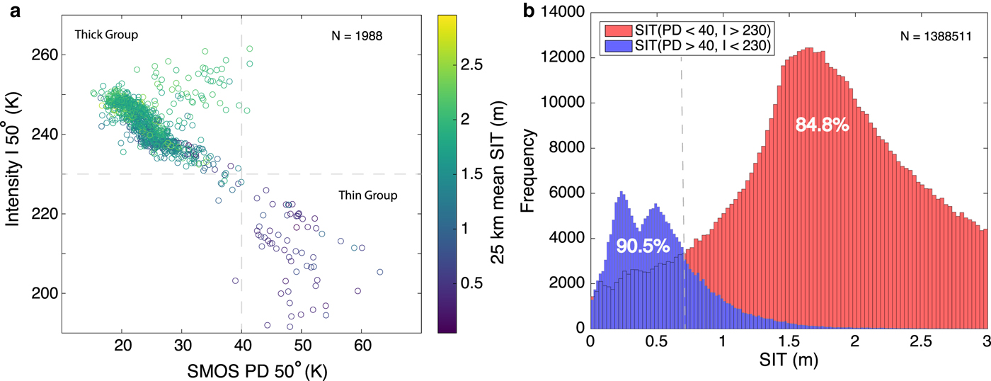
A sensitivity analysis by linear regression between various brightness variables (i.e. TB at horizontal (H) and vertical (V) polarization, First Stokes intensity or simply intensity I, and PD) shows that PD has a maximum correlation with the ASIT (Table 3). Two distinct groups have been identified based on the intensity and PD at 50° incidence angle (Fig. 2a).
Sensitivity analysis (linear regression) between SMOS TB at 50° incidence angle and ASIT (<3 m) (TBI = First Stokes intensity, TBV = vertical polarization, TBH = horizontal polarization, PD50 = polarization difference)
(a) Scatter plot of SMOS intensity (I) versus PD at 25 km grid for selected dates in March and April of 2011–15. The color bar shows the mean SIT value at 25 km grid (N = 1988). Vertical and horizontal dashed lines separate thin and thick SIT groups. (b) Histograms of two groups of original, unaveraged SIT (i.e. thin and thick, which are based on criteria as shown in the top left corner of the panel) (N =1 388 511). The vertical dashed line shows SIT where thin and thick SIT signatures merge. A 90.5% of the thin SIT data (blue histogram) belongs to thin SIT group, while 84.8% of thick SIT data (red histogram) belongs to thick SIT group.
The collocation of SMOS TB, ASIT, SIC and various SIT products is a very important step in the algorithm development. All datasets are collocated to SMOS (Gabarro and others, Reference Gabarro, Turiel, Elosegui, Pla-Resina and Portabella2017). A simple computational approach is applied for re-gridding other products (UBremen, UHamburg and OSI SAF SIC) onto the 25 km EASE grid using linear 2D-interpolation. The ASIT data are converted from geographic coordinates to North azimuthal equal-area map with 25 km resolution pixel (EASE grid or NL) by simple calculation (for details see https://nsidc.org/data/ease/ease_grid.html). Each 25 km cell contains several SIT values, i.e. an SIT distribution with a mean and an std dev. The mean value of all those ASIT values that fall inside a 25 km × 25 km gridcell is taken. This gives one SIT value per 25 km grid. This method effectively uses the sparse and limited amount of airborne thin SIT data to provide collocations at a more comparable spatial resolution to that of SMOS. The filled coastline data from the Global Self-consistent Hierarchical High-resolution Geography (GSHHG) dataset have been used as a land mask with a stereographic projection of North Polar regions and oblique Mercator projection.
3.2 Weighted non-linear curve fitting
All ASIT and SMOS PD data used for the curve fitting belong to grids with collocated OSI SAF SIC. The collocated ASIT and SMOS PD data that fall below 60% SIC have been rejected from this analysis. A cut-off of 60% SIC is chosen carefully after performing a sensitivity analysis between ASIT and SIC at 25 km grid. Now, the methodology for retrieving SIT using PD of SMOS TB at 50° incidence angle is introduced. The PD50 is defined as the difference between SMOS TB at H- and V-polarization at 50° incidence angle (Eqn (1)),
 $${\rm PD}50 = {\rm TBV}(50)-{\rm TBH}(50),$$
where TBH(50) and TBV(50) are TB values at H- and V-polarization at 50° incidence angle. It is already known that the TB is exponentially related to the SIT (Kaleschke and others, Reference Kaleschke, Maaß, Haas, Heygster and Tonboe2010, Reference Kaleschke, Tian-Kunze, Maaß, Mäkynen and Drusch2012). The SMOS PD data are fitted to the airborne measurements of SIT with a hyperbolic tangent curve as follows (Eqn (2), Fig. 3),
 $${\rm PD}50 = a + b\; {\rm tan}h\left( {\displaystyle{d \over {d_0}}} \right).$$
where d is SIT, a, b and d 0 are constants.
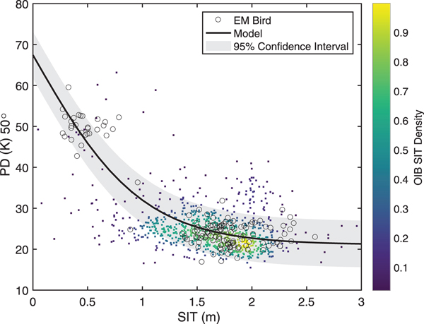
Model fit between SMOS PD at incidence angle 50° and ASIT from EMB and OIB campaigns during March and April of 2011–15. The density of OIB SIT is shown on a color scale.
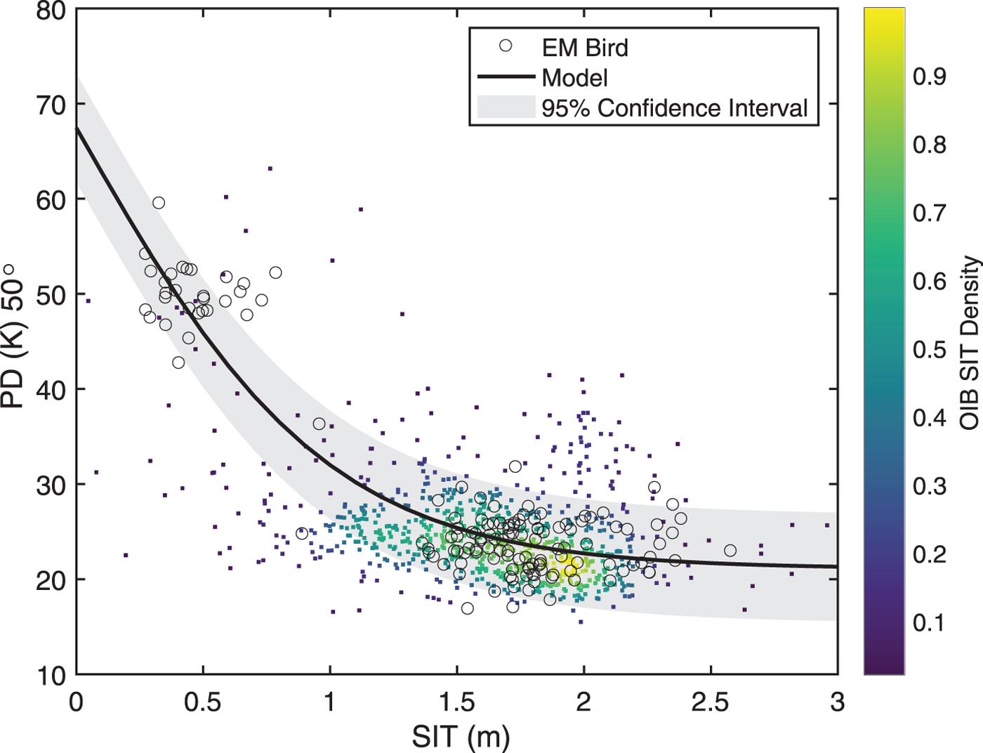
The EMB and OIB SIT data have been used for obtaining Eqn (2). As the available accuracies from two different data sources are 0.10 and 0.40 m, respectively; all values of OIB SIT are assigned a weight of 0.0625 (i.e. 1/16). The constants a = 67.4413, b = −46.3496 and d 0 = 0.9919 m. d 0 is the maximum retrievable SIT by this algorithm. The Pearson's r = 0.6277 for modeled PD versus SMOS PD. Figure 3 shows the scatter plot of EMB and OIB SIT data with non-linear curve fitting at 95% confidence interval. The color shows the density of OIB SIT data.
The Pearson and Spearman correlation coefficients are computed for modeled PD and SMOS PD. These details are presented in the Results (Section 4).
4. RESULTS
4.1 Rationale
The analyses start with a large amount of ASIT data acquired over 5 years' time span (2011–15) under different field campaigns, which include the year (2012) of lowest recorded Arctic sea-ice extent (Parkinson and Comiso, Reference Parkinson and Comiso2013), and a period (2013–14) of increase in sea-ice volume (Tilling and others, Reference Tilling, Ridout, Shepherd and Wingham2015). The airborne data cover a large variability of SIT and SIC in the Arctic, wide geographic distribution and SIT distribution from freeze-up to winter maximum of March (Fig. 1).
A reasonable relationship between SIT and PD (in TB) can be achieved if there is a substantial variability in SIT at corresponding unscaled TB. The use of thin SIT data from EMB with accuracy 0.10 m and thick SIT data from OIB with accuracy 0.40 m allows a reliable retrieval of SIT using SMOS TB (Fig. 2). Here, the thin and thick SIT groups in the data are defined based on the PD and intensity limits of each group. The EMB data contain some, though very few, number of thick SIT data points; and OIB data contain predominantly thick SIT data points with a small number of thin SIT data points. It can be intuitively defined from the scatter plot in Figure 2a, that PD > 40 K and I < 230 K is thin SIT group, and PD < 40 K and I > 230 K belong to thick SIT group (marked by vertical and horizontal dashed lines in Fig. 2a). A 90.5% of the thin SIT data (blue histogram in Fig. 2b) belongs to the thin SIT group, while 84.8% of thick SIT data (red histogram) belongs to thick SIT group (Table 4). The thin sea ice has an approximate PD range of 40–50 K and intensity between 190 and 220 K. The overlapping SIT (a vertical dashed line in Fig. 2b) gives a preliminary indication of upper bound of SIT to be computed, which is ~0.7 m.
Distribution of points within thin and thick groups (intensity, I versus polarization difference, PD). Incidence angle = 50°; thresholds: PD = 40 K, I = 230 K (Fig. 2)

4.2 Retrieval of the SIT
After establishing a non-linear relationship between SMOS PD and SIT (Eqns (1) and (2)), one can obtain the SIT for a given location and date by inverting Eqn (2). The inverted Eqn (2) becomes,
 $$d = d_0\; {\rm tan}h^{-1}z,$$
 $$z = \displaystyle{{{\rm PD}50-a} \over b}.$$
As the SIT (d) cannot be negative, only those values of tanh(d/d 0) are retained that lie between 0 and 1, i.e. the positive quadrant. This range also removes any imaginary numbers resulting from the tanh −1z and negative values of SIT (Eqns (3) and (4)). The maximum and minimum values of inverse hyperbolic tangent set the maximum and minimum limits of PD. Thus, 0 <z <1 gives 21.1K <PD50 <67.4K (rounded values to one decimal place). It is known from trigonometry that tanh −1(0) = 0 and tanh −1(1) = ∞; and tanh−1z <1, one can obtain 0 <d <0.9919 m. Thus, the retrievable BEC SIT values are <~0.99 m. This renders any SIT value higher than 0.99 m physically meaningless, and therefore, treated as the maximum in the SIT map. The proposed algorithm (hereinafter: BEC algorithm), by hyperbolic tangent properties, significantly limits the retrieval of SIT for regions where SIC is low as will be explained in Section 5.
4.3 Algorithm performance and SIT error
It is important to include different sea-ice representations, i.e. thin and thick SIT, for fitting a model with PD. This is to include the true sea-ice representation of all types. Thin SIT from EMB and thick SIT from OIB form a near ideal dataset for curve fitting (Fig. 3). Due to different instrumentation and acquisition techniques related to airborne thin and thick SIT, their accuracies differ from each other. Despite having different accuracies, it is possible to capture the true SIT response to TB using these datasets. It was described in the previous paragraph that there was a little overlap between the thin and thick SIT groups; this leaves a known region of little density between the thin and thick SIT groups (Ricker and others, Reference Ricker2017) (Fig. 3). This region (~0.5–1 m or so) is predominantly visible during March but is almost absent in the early freeze-up in November. A priori knowledge of a non-linear (exponential) dependence of SIT on TB is available from Kaleschke and others (Reference Kaleschke, Maaß, Haas, Heygster and Tonboe2010). The proposed hyperbolic tangent function fitting of PD with SIT is shown in Figure 3. The maximum PD value, 67.4 K occurs at zero SIT, and the magnitude of PD decreases as the SIT increases. The PD reaches the saturation at 21.1 K (see Eqn (2)), below which the increasing SIT does not make any change in the PD. Huntemann and others (Reference Huntemann2014) have reported the maximum value and saturation limit of PD as 51 and 20 K, respectively, which showed a dynamic range of 31 K. The PD range of 46 K using BEC algorithm makes it possible to effectively retrieve SIT from hyperbolic curve fitting. A narrow confidence interval for thin SIT indicates thin SIT prediction with greater confidence than thick SIT (Fig. 3).
The BEC algorithm predicts SIT in 0–0.99 m range with an RMSE of 0.10 m, which seems reasonably good for analysis at a 25 km grid. The main advantage of this result lies in the fact that the ambiguities between passive microwave emission contributions due to low SIC and thin SIT have been excluded. Where it is not possible to decipher TB from low SIC and thin SIT, the BEC algorithm simply rejects such regions. This is manifested in the regions of thin SIT and intermediate SIT (~0.8–1.4 m or so). A known gap in data points between 0.7 and 1.5 m is noticeable in Figure 4. One of the reasons for this gap is averaging SIT values at 25 km EASE-grid, on which SMOS PD data have been generated. Ricker and others (Reference Ricker2017) also showed this gap at 25 km EASE-grid when plotting CryoSat-2 (thick) and SMOS (thin) SIT. The gap becomes noticeable during March when most ice is thicker than 1.5 m except in the vulnerable regions of the circumpolar Arctic.
Validation of BEC SIT with exclusive ASIT (0–3 m) acquired from EMB campaigns (See Table 2) during March 2014 and April 2015.
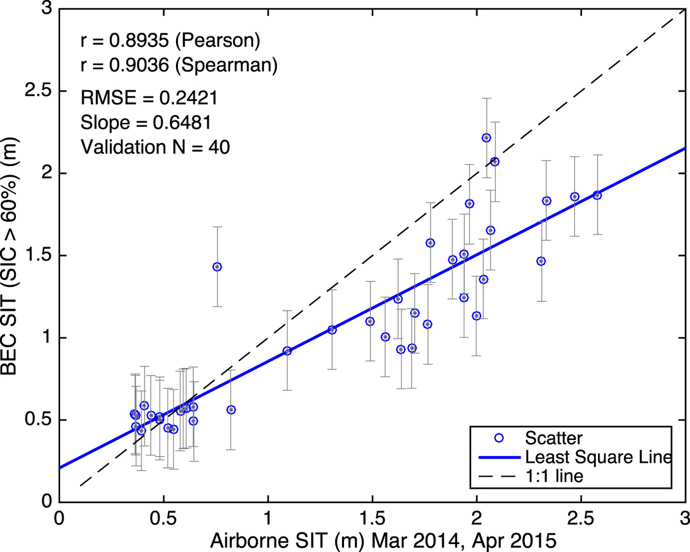
It is clear from Figure 4 that BEC SIT is biased above 1.5 m, and the algorithm underestimates the ground truth. The BEC SIT computed for thickness 0–3 m has an RMSE of 0.24 m with the ground truth and the maximum retrievable SIT is <0.99 m. Thus, BEC algorithm predicts SIT in the range 0–0.99 m with 10.5% error and SIT in the range 0–3 m with 24.4% error in it.
4.4 Validation of BEC SIT
The BEC SIT is validated for a full range of SIT 0–3 m to examine the predictive capability of BEC algorithm for thick ice, even though the SIT values >0.99 m are physically meaningless as explained above. Figure 4 shows the results of the validation of BEC SIT with corresponding collocated ASIT for March and April of 2014–15 for high OSI SAF SIC. The value of Pearson's r = 0.89, Spearman's r = 0.90, RMSE of LS fit (for SIT 0–3 m) = 0.24 m and the slope of the regression line (shown in solid blue) is 0.65. The total number of independent (validation) points available for LS regression, for which corresponding BEC SIT (in the range 0–3 m) exists, is 40. The identity line (1:1) is plotted as the black dashed line. It is clear from Figure 4 that BEC algorithm underestimates thick sea ice (~1.5 m or greater). The RMSE of 0.24 m of SIT retrieval in the range of 0–3 m seems reasonably good in the BEC algorithm.
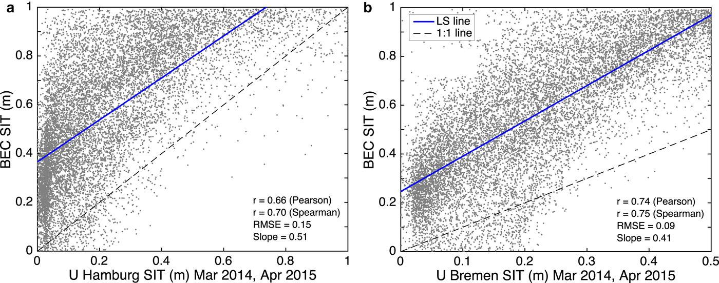
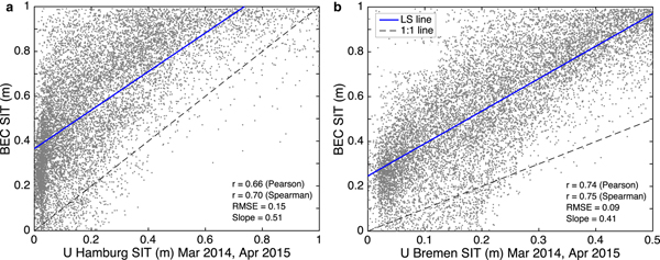
The BEC SIT product is compared with other SIT products to assess and verify relative performances. Figure 5 shows the performance of BEC SIT in comparison to UHamburg SIT and UBremen SIT for the same dates in March and April of 2014–15 from which BEC algorithm is generated. A linear regression (blue solid line in Fig. 5a) between BEC SIT and UHamburg SIT shows Pearson's r = 0.68, and Spearman's r = 0.71, RMSE = 0.15 m and the slope of 0.52. The BEC algorithm largely overestimates SIT when compared with UHamburg SIT but is statistically correlated well with UHamburg SIT. A linear regression (blue solid line in Fig. 5b) between BEC SIT and UBremen SIT shows Pearson's r = 0.74, and Spearman's r = 0.75, RMSE = 0.09 m and the slope of 0.41. BEC SIT departs significantly from UBremen SIT and shows highly biased and overestimated SIT values. A detailed account of this SIT comparison is provided in the Discussion (Section 5).
Scatter plot comparison of BEC SIT with (a) UHamburg SIT, (b) UBremen SIT for validation dates given in Table 2. The data correspond to the entire Arctic Ocean for each SIT product on the specified dates. The black line is 1:1. LS line is shown in blue color.
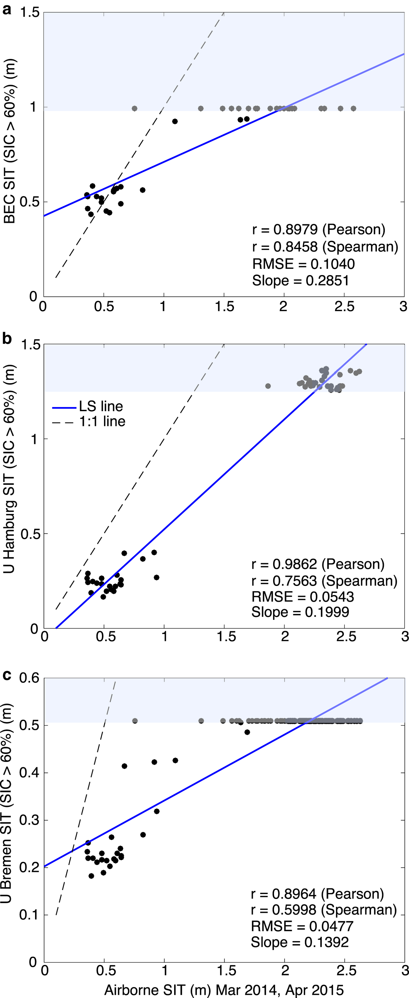
An individual statistical investigation of the three SIT products using the exclusive validation ASIT data for high OSI SAF SIC gives similar results as described in the above paragraph. In Figure 6, the black broken line is the identity line (1:1), the blue solid line is the linear regression between different SIT products and ASIT. All three algorithms give biased results for SIT >1 m. This supports an earlier statement that BEC SIT >0.99 m are physically meaningless, and other SIT products also show high error in SIT values >1 m. This elaborates one of the reasons why the SIT has been validated in the range 0–3 m (see Fig. 4) instead of 0–0.99 m, i.e. the performance evaluation. The computed SIT beyond the maximum retrievable SIT by an algorithm is shown as shaded region (in blue) in Figure 6. The re-gridding of UHamburg and UBremen SIT at 25 km grid degrades the computed SIT with a loss of information. The SIT values from UHamburg and UBremen algorithms considerably depart from the identity line (1:1) and underestimate thin SIT as compared to BEC algorithm at 25 km original SMOS grid. The maximum retrievable SIT by BEC algorithm is 0.99 m and the RMSE for BEC SIT values ranging between 0 and 0.99 is 0.1040 m (as shown in Fig. 6a), i.e. with 10.5% error of prediction. Coincidently, the accuracy of BEC SIT product is almost akin to the accuracy of EMB data, i.e. 0.10 m (Haas and others, Reference Haas, Lobach, Hendricks, Rabenstein and Pfaffling2009). The RMSEs for UHamburg (for 0–1.2 m) and UBremen SIT values (for 0–0.55 m) after re-gridding at 25 km are 0.0543 and 0.0477 m, respectively (Figs 6b and c).
A validation comparison of SIT (a) BEC, (b) UHamburg and (c) UBremen. The ASIT validation data used are from the dates given in Table 2. The black line is 1:1, and the regression line is shown in blue color. Blue-shaded region represents SIT that are not retrievable by a given algorithm (see Section 4.4 for explanation).
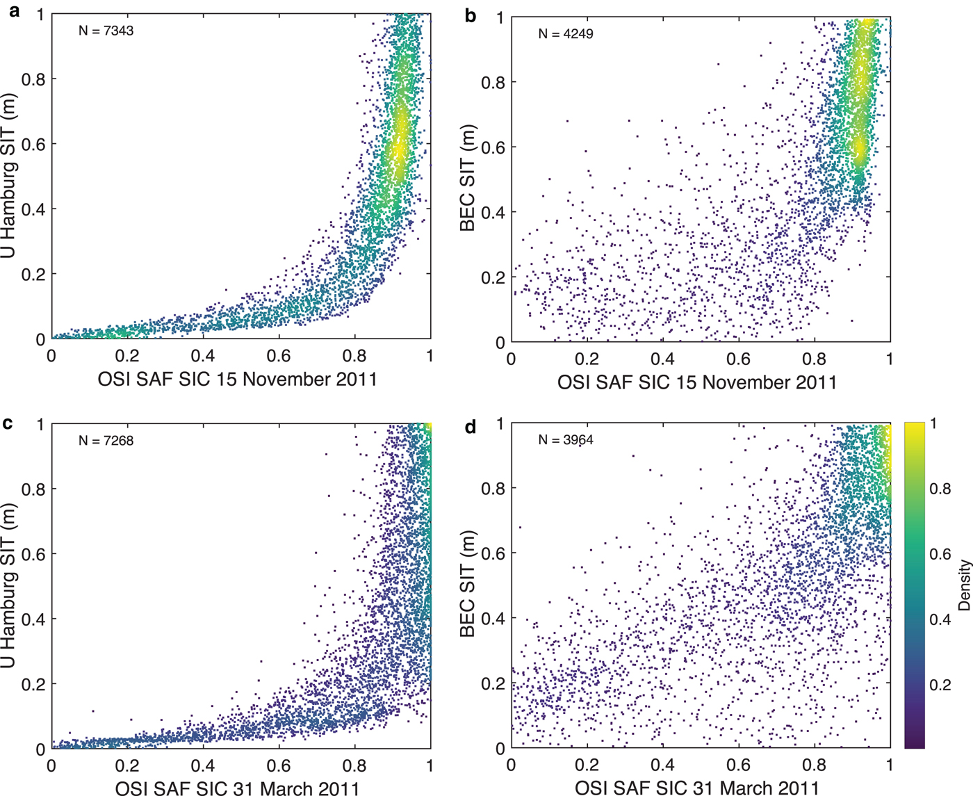
The BEC SIT versus OSI SAF SIC have been plotted for algorithm training dates (March and April of 2011–2015) and exclusive validation dates (March and April of 2014–15) to show that BEC SIT corresponds to high SIC (Table 2, Fig. 7). For validation dates, the BEC SIT corresponds to SIC above 80%. Extending this analysis from training and validation dates to any given date during winter, a performance analysis of BEC SIT and UHamburg SIT for 15 November 2011 (freeze-up onset) and 31 March 2011 (winter maximum) (Fig. 8) is attempted. Figure 8 shows a distinct relationship between SIT and SIC. This important result is discussed at length in the following Section 5. A graphical comparison of the three SIT products and corresponding OSI SAF SIC on during freeze-up clearly assesses the relative performances of SIT algorithms (Figs. 9–11).
Scatter plot showing BEC SIT for corresponding OSI SAF SIC during March and April. (a) Algorithm training data during 2011–15, (b) validation data during 2014–15 (Table 2).

Density plots of SIT derived using the UHamburg algorithm (Tian-Kunze and others, Reference Tian-Kunze2014) (a, c) and BEC SIT (b, d) against OSI SAF SIC on 15 November (a, b), and 31 March (c, d), 2011. The modes corresponding to the lowest and highest SIT are removed.
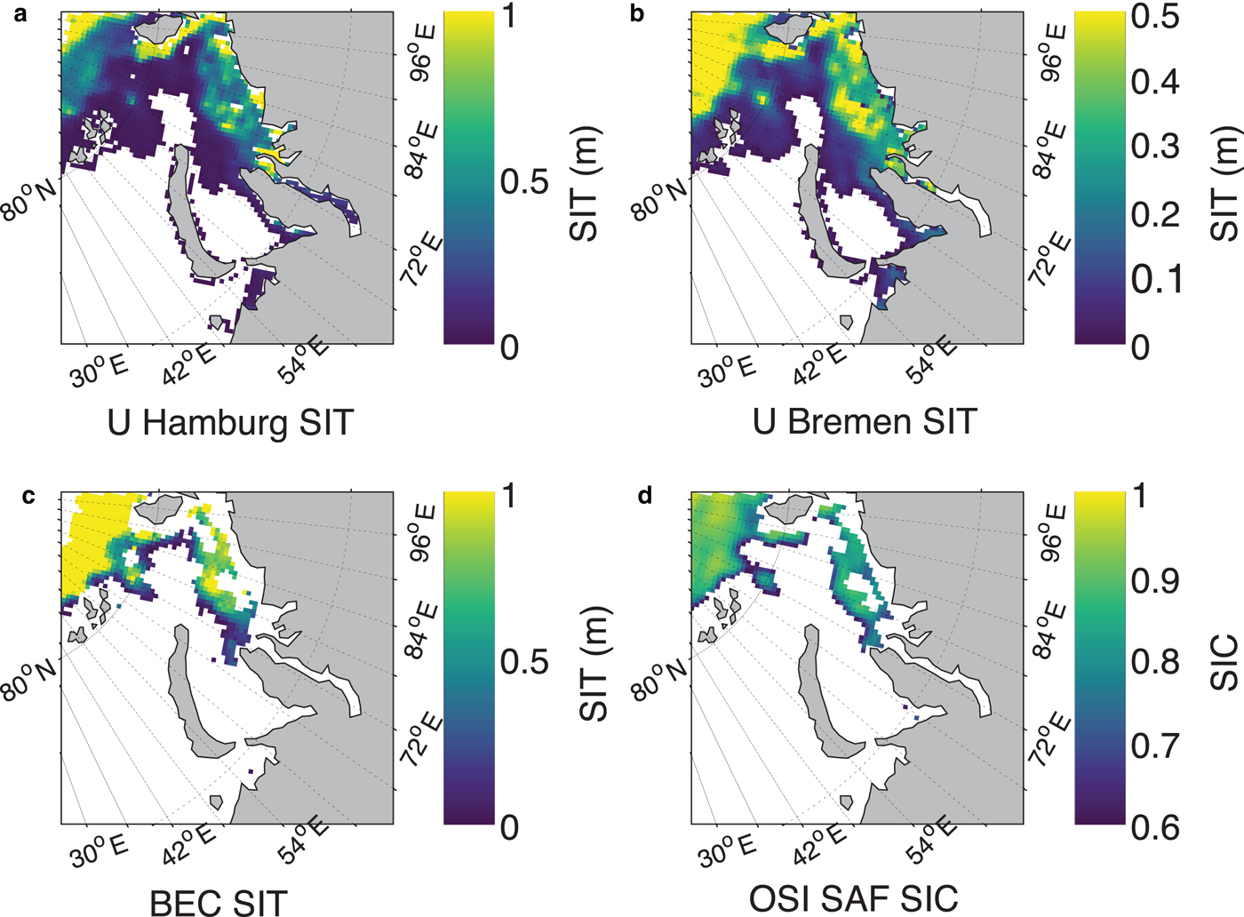
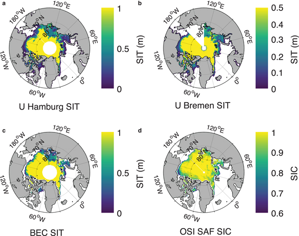
A visual comparison of SIT products from (a) UHamburg, (b) UBremen, (c) BEC and (d) OSI SAF SIC on 3 November 2014. SIT color scale shows the range of zero to maximum retrievable SIT by an algorithm.

A zoomed comparison of the performance of various SIT products at 25 km grid with respect to prevailing SIC conditions on 24 November 2015, in the Kara Sea region of Russian Arctic. (a) UHamburg SIT, (b) UBremen SIT, (c) BEC SIT and (d) OSI SAF SIC. SIT color scale shows the range of zero to maximum retrievable SIT by an algorithm.
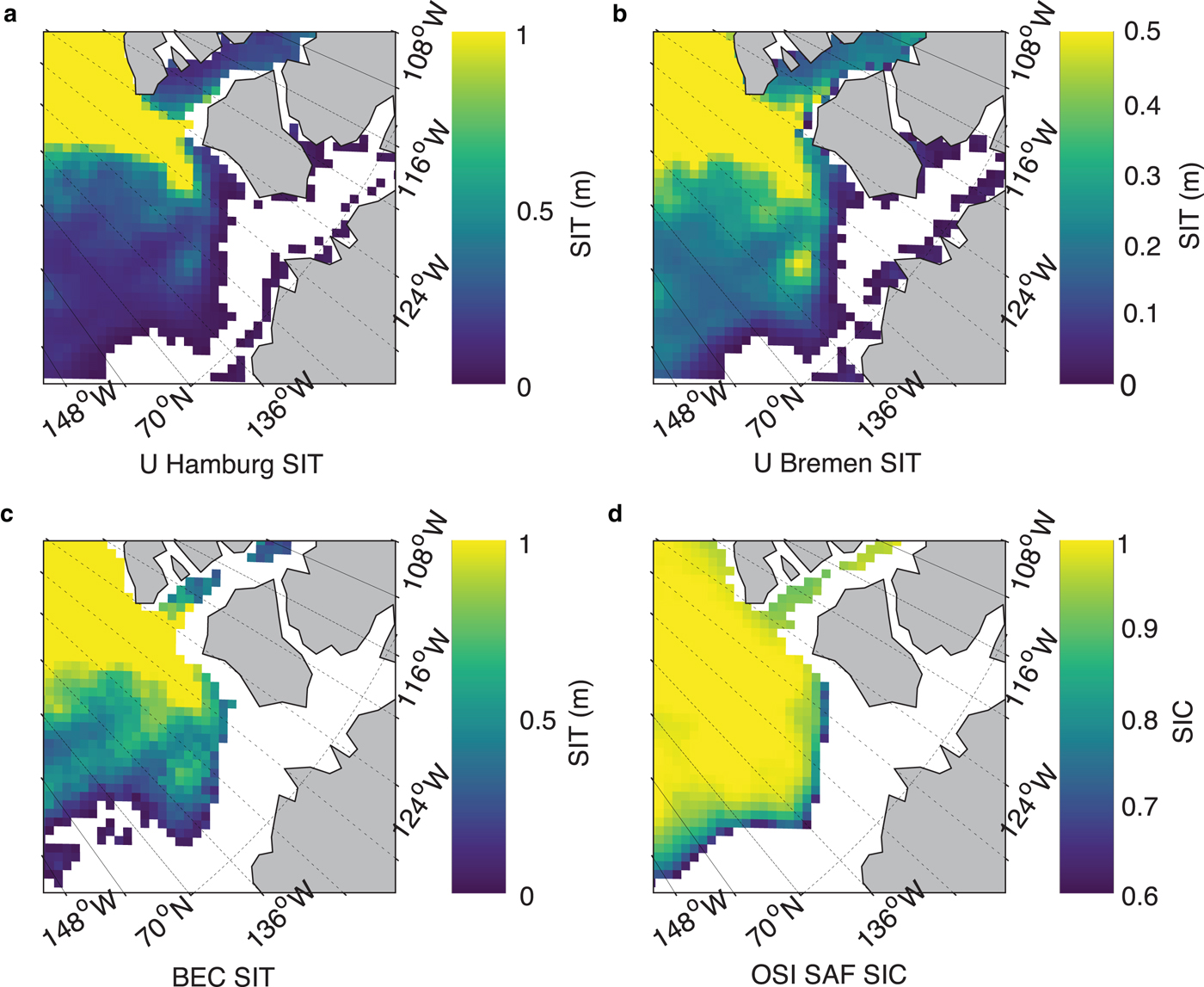
A zoomed comparison of the performance of various SIT products at 25 km grid with respect to prevailing SIC conditions on 20 October 2015, in Beaufort Sea of Canadian Arctic. (a) UHamburg SIT, (b) UBremen SIT, (c) BEC SIT and (d) OSI SAF SIC. SIT color scale shows the range of zero to maximum retrievable SIT by an algorithm.
5. DISCUSSION
5.1 Assessment with other SIT products
It is important to compare BEC SIT product with other available SIT products to assess its relative performance and advantages/disadvantages. Figure 5 shows BEC SIT compared with UHamburg and UBremen SIT computed for same dates in March–April of 2014–15 for which algorithm training is performed. It is obvious from the line of equality that BEC algorithm overestimates SIT in comparison to both other SIT products. When validating each SIT product with exclusive validation ASIT, the individual performance of algorithms at 25 km EASE-grid can be clearly compared (Fig. 6). A noticeable gap of ~0.8–1.4 m is observed in all three SIT products. Although the UHamburg and UBremen algorithms seem to provide reasonable thin SIT predicted values at 12.5 km, they highly underestimate SIT for all thickness ranges at 25 km grid. The BEC algorithm, however, underestimates only thick SIT and estimates thin SIT with a reasonable error.
The BEC algorithm significantly limits the prediction of SIT for the regions where there is ambiguity in TB for low SIC and thin SIT. This means that the BEC algorithm rejects the pixels where it is not possible to discriminate the TB signatures whether it is due to thin SIT or partial SIC within 25 km grid. None of the previous SIT algorithms addressed this issue and incorrectly provide thin SIT where partial SIC is present. The BEC algorithm exclusively addresses this major problem and considers only those points with SIC >60% for algorithm training (Fig. 7). The SIC threshold for 25 km SMOS EASE grid is intuitively chosen based on field experience. Even though the BEC algorithm predicts SIT for regions of all SIC (0–100%), regions of low SIC are significantly limited as seen in Figure 8. The core density of BEC SIT lies above 80% of SIC (the modes caused by zeros and maximum saturated values are removed) for both early freeze-up (November) and winter maximum (March). One can observe that during winter maximum in March, the highest density of BEC SIT values lies above 80% SIC whereas UHamburg SIT density is spread under low SIC (Fig. 8). This is because BEC SIT does not give any SIT value for those pixels with low SIC. A high scatter is observed in BEC SIT density plot due to a purely empirical approach of SIT retrieval.
Figure 9 shows a graphical representation of various SIT products vis-à-vis OSI SAF SIC during the freeze-up period on 3 November 2014. A lot of thin SIT and a mix of open water and sea ice (i.e. marginal ice zone (MIZ)) are observed offshore and at the ice edges. It is known that SMOS TB values in the proximity of land (~200 km from the edge of land) are contaminated by TB contributions from land (Martín-Neira and others, Reference Martín-Neira2016). It can be seen from Figure 9c that all along the land-ocean boundary there are no data (exceptions excluded) regardless of whether it is sea ice or seawater. This is most likely due to the combined presence of low SIC pixels and thin SIT at the land–sea and ice–water boundaries since only the TB data that are not corrected for the land–sea contamination have been used. Due to above reason, BEC algorithm automatically omits parts of areas of close proximity to the land while other SMOS SIT products (i.e. UHamburg and UBremen) do not consider to remove this effect (Fig. 9a and 9b). The BEC SIT product matches very well with the OSI SAF SIC of 80% or above (Fig. 9d). A zoomed comparison of the performance of all SIT retrievals has been shown in Figure 10 with prevailing SIC conditions in the Kara Sea region of Russian Arctic on 24 November 2015. It is evident from the figure that the BEC algorithm significantly limits the SIT retrieval in the regions of partial SIC. The similarity of common regions of SIC and BEC SIT is also evident in Figure 11 from the southern Beaufort Sea region of the Canadian Arctic on 20 October 2015. The omission of BEC SIT at the proximity to land and low SIC can be seen in Figure 11c.
6. CONCLUSION
In this paper, a new method for SIT retrieval from the PD of SMOS TB was presented. The BEC algorithm overcomes many difficulties that previous SIT products did not consider. These are summarized as follows:
(1) For the first time, only airborne data are used for algorithm training to retrieve the SIT from PD of SMOS TB. Other products use sea-ice model-based algorithms to retrieve SIT, which requires the knowledge of some auxiliary variables (temperature and salinity of the ice, the temperature of the air, etc.), whose errors are propagated onto the SIT retrievals.
(2) The BEC algorithm, by a hyperbolic function, rejects the regions having TB signatures of coincident marginal SIC and thin SIT. One of the most important unresolved issues in SIT retrieval using passive microwave radiometry is the ability to separate TB signatures from thin SIT and low SIC regions. One cannot discern them from the TB and/or its PD measurements. The UHamburg and UBremen algorithms neither resolve this issue nor filter such data, and thus provide incorrect retrieved SIT in the regions of low SIC.
(3) SMOS TB values without interpolation at 25 km EASE-grid are used. This is expected to improve the quality of SIT retrieval. Other SIT algorithms have interpolated SMOS TB to a 12.5 km grid compromising with the true TB response to SIT. The BEC algorithm can only be used for SIT below 0.99 m for which the RMSE is 0.10 m with a prediction error of 10.5%.
The fact that SIT can be retrieved from the SMOS TB has been well-received by the scientific community. However, this has certain limitations of its own. On the one hand, sensor limitations: (1) the information beyond certain spatial resolution is unavailable, which is 25 km grid for SMOS TB; and (2) the choice of microwave frequency for penetration depth in sea ice (low frequencies allow deeper investigation). On the other hand, the following geophysical limitations impact the TB and pose a problem for current SIT retrievals: snow roughness, ice surface roughness, ice thickness distribution, ice salinity, ice temperature, discrimination between thin SIT and low SIC, and others. These geophysical limitations leave a big gap in the proper understanding of the sea-ice characteristics at both the 25 km grid and the sub-grid levels. The BEC algorithm represents, however, a new step towards optimal SIT estimates by filtering SIT data under low SIC conditions. The averaging of ASIT at 25 km results in very few collocations in the range of 0.8–1.4 m due to the reduction in the number of data points. This SIT range seems to be a vulnerable range which has very small residence time compared to other thickness ranges. More collocations are therefore needed to consolidate the SIT model function. There is a need to acquire thin SIT field data during freeze-up, i.e. November–December before sea-ice advances from thin to thick ice. It would then be possible to capture more data in the vulnerable SIT range of 0.8–1.4 m at 25 km resolution, which would in turn lead to improved SIT retrievals from spaceborne passive microwave radiometry.
An operational SIT product in netCDF format, which includes a reprocessing for the past 9 years (SMOS mission lifetime) has been generated, and will be made available for (freely) registered users at bec.icm.csic.es by mid-2019. The registered users will be able to browse through product images and make area-based selection enquiry on a graphical visualization platform.
ACKNOWLEDGEMENTS
This work was supported in part by the Ministry of Economy and Competitiveness, Spain and in part by FEDER EU through the National R + D Plans PROMISES Project under Grant ESP2015-67549-C3-2-R and L-Band Project under Grant ESP2017-89463-C3-1-R. We thank the director of ICM-CSIC, Josep Lluis Pelegrí for encouragement and support. We thank the entire BEC team for useful discussions and technical help. We are thankful to Dr Stefan Hendricks of the Alfred Wegener Institute (AWI) for providing airborne EMB SIT data for 2011 and 2015. We gratefully acknowledge the following field campaigns for making the airborne SIT data available: SIZONet, NASA Operation IceBridge, ESA SMOSIce, TD XX and N-ICE.


 Open access