


1. Introduction
Global wind power has grown rapidly in recent years. For instance, 116.6 GW of new wind power capacity bringing the total installed capacity up to 1021 GW in 2023. On the one hand, it is known that wind power is a kind of clean energy that can reduce carbon emissions by replacing fossil energy. For example, a total of 837 GW of global wind energy installed capacity generated about 2186 TWh of electricity which is 1311 Mt of carbon dioxide (CO2) mitigation in 2021 (Long et al., Reference Long, Chen, Xu, Li and Wang2023). Also, wind power will reduce the NOX, SO2, as well as VOC emissions from outside the region coming from fossil-fuel-fired power plants (Ruan et al., Reference Wang, Luo, Wu and Fan2022). On the other hand, wind power also has a direct impact on the climate, such as wind speed, temperature, humidity, atmospheric boundary layer, precipitation, etc. (Keith et al., Reference Keith, DeCarolis, Denkenberger, Lenschow, Malyshev, Pacala and Rasch2004; Miller & Keith, Reference Mangara, Guo and Li2018; Saidur et al., Reference Saha, Moorthi, Wu, Wang, Nadiga, Tripp, Behringer, Hou, Chuang and Iredell2011) and even the resultant air pollution responses.
To date, in situ observations, satellite remote sensing, and both global and regional numerical models have been used to investigate the impacts of wind power. Wind farms alter the atmosphere by increasing surface roughness (Baidya Roy, Reference Baidya Roy2004), extracting momentum and adding extra turbulence (Xia et al., Reference Xia, Zhou, Freedman, Roy, Harris and Cervarich2019), inducing wakes (Wang et al., Reference Wang, Luo, Wu, Tan, He, Ye and Fan2019), and even changing the climate (Abbasi et al., Reference Abbasi, Tabassum and Abbasi2016; Fitch, Reference Fitch2015; Miller & Keith, Reference Mangara, Guo and Li2018; Sun et al., Reference Su, Li and Kahn2018). For instance, wind farms in west-central Texas in the US were found to warm the surface temperature in winter by 0.72 ℃/decade (Zhou et al., Reference Zhao, Li, Zhang, Yang and Liu2012), while European wind farms (Vautard et al., Reference Tomaszewski and Lundquist2014) and Chinese wind farms (Sun et al., Reference Su, Li and Kahn2018) change the surface temperature within ±0.3 ℃ and ±0.5 ℃, respectively, under various scenarios. Also, these impacts are related to the factors, such as atmospheric stability (Liu & Stevens, Reference Liu and Stevens2021; Wang et al., Reference Wang, Luo, Ming, Mu, Ye and Fan2022), inter-farm cluster interaction (Wang, Luo, Wu, et al., Reference Wang, Luo, Wu, Mu, Tan and Fan2023), topography (Yan et al., Reference Xueting, Jinxin, Zhenghong, Fei and Yang2018), and sea surface (Wu et al., Reference Wang, Shao, Zhang, Liu, Zou and Xiao2022). As air pollution is related to meteorological conditions, it is of great interest to understand how wind power influences air pollution redistribution, which is caused by the climatic impact.
Since 2008, China has been the global leader in the wind market, with a total capacity of 211 GW at the end of 2018, accounting for 36% of the total installed capacity. This number will further increase to 1,000 GW by 2050, and thus, wind power will serve as one of the most important power sources to achieve carbon peak and carbon neutrality goals (Institute, E.R., 2011). Evidence indicates that large wind clusters in northern China alter the regional planetary boundary layer height (PBLH) (Wang et al., Reference Papanastasiou, Melas and Lissaridis2019), which directly influences air pollutant concentrations (Li et al., Reference Li, Zhang, Cai, Song and Zhu2021). Since 2013, air pollution has been a serious public issue in China, especially in northern China (Guo et al., Reference Guo, Hu, Zamora, Peng and Zhang2014; Zhang et al., Reference Zhang, He and Huo2019). It is thus of significant importance to understand the climatic impacts and the resultant air pollutant responses induced by the Chinese wind power (CWP) on a national scale.
Here, we investigate the impacts of a realistic scenario of Chinese wind farms on local and regional climate and air pollution by using dynamic numerical weather predictions and a multiscale air quality model for the first time. Utilizing the available locations and cumulative capacity of wind farms in each province, we establish a dynamic wind farm fleet scenario in China from 2009 to 2018. This scenario offers a realistic portrayal of the explosive expansion of the wind power industry, alongside the significant air quality issues the country has encountered. The influence of a wind turbine on the atmosphere is represented by the momentum sink and turbulent kinetic energy (TKE) source in the region crossed by a turbine rotor with a wind farm parameterization (WFP) (Fitch, Olson, et al., Reference Fitch, Olson and Lundquist2013) in the Weather Research and Forecasting (WRF) model (Skamarock et al., Reference Saidur, Rahim, Islam and Solangi2008), and the Community Multiscale Air Quality (CMAQ) model (Byun & Schere, Reference Byun and Schere2006) is applied to investigate these impacts on both climate and air pollutants. The remainder of this paper is organized as follows: Section 2 introduces the materials and methods, including wind power development in China, experimental design, model configurations, wind farm parameterization, and WRF-CMAQ model validation. Section 3 shows the results of the impacts of Chinese wind farms on climate and air pollutants under the dynamic fleet scenario, i.e., seasonal, diurnal, and long-term impacts, also the underlying physics is analyzed and discussed, which is followed by the discussion and implications in Section 4.
2. Materials and methods
2.1. Wind power development in China
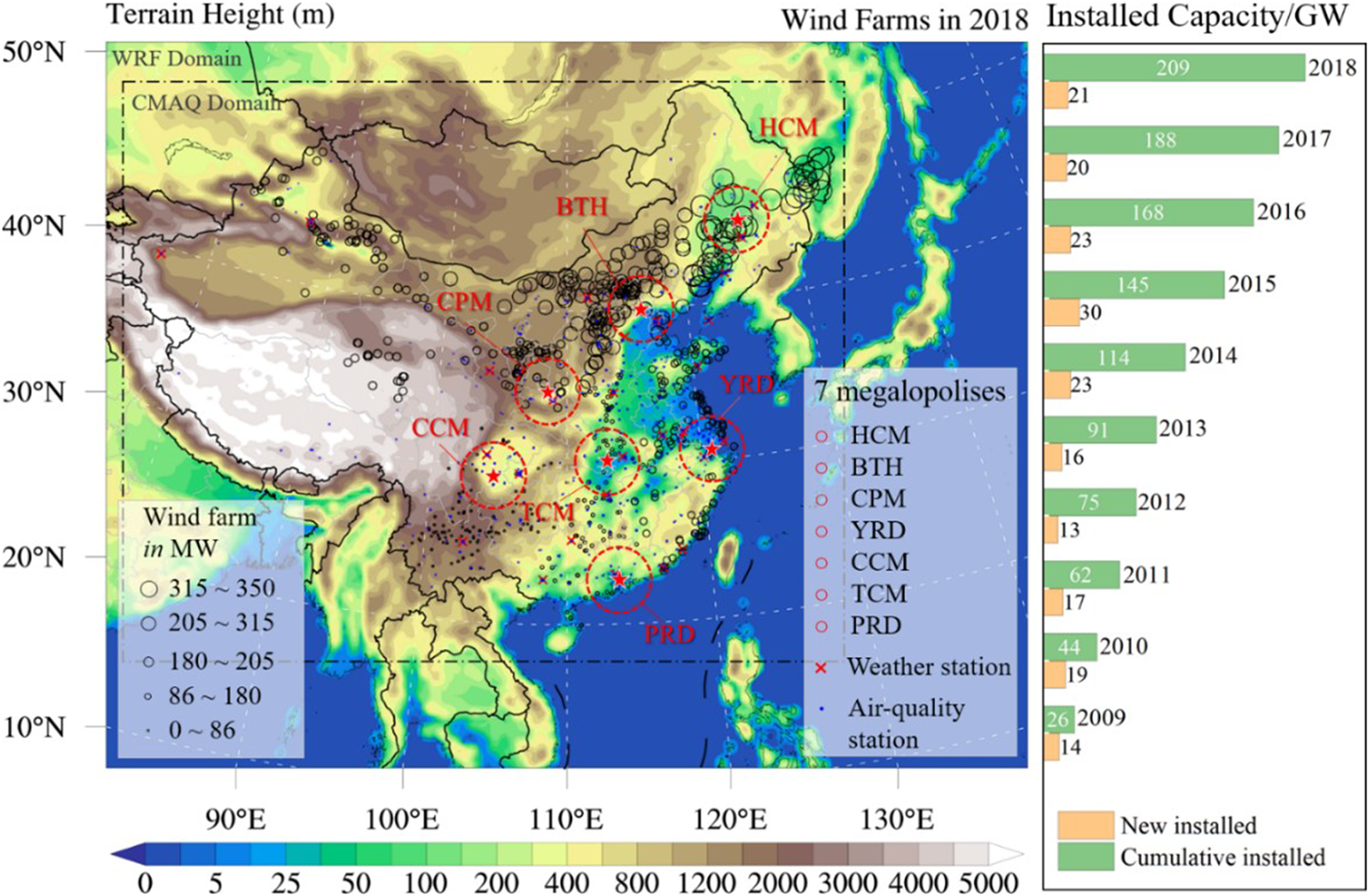
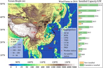
Wind power development in China started as early as the 1980s and progressed in three stages, i.e., the demonstration stage (1986–1993), the industrialization promotion stage (1994–2005), and the scaling-up stage (2006 onwards) (X. Zhao et al., Reference Zhao, Zheng, Wang, Smith, Lu, Aunan, Gu, Wang, Ding, Xing, Fu, Yang, Liou and Hao2016). During the scaling-up stage, the Renewable Energy Law was released in 2006 and revised in 2009. China has undergone explosive growth in wind power: six onshore gigawatt-scale wind power clusters have been erected in northern China, and a near-offshore wind cluster has been constructed in the coastal Jiangsu Province. The accumulated installed capacity of wind power rapidly rose from 26 GW in 2009 to 209 GW in 2018. The distribution of Chinese wind farms in 2018 and the accumulated installed wind power capacity from 2009 to 2018 are illustrated in Figure 1. The left panel map with Lambert projection shows the WRF and CAMQ domains. Each black circle represents a wind farm with various capacities, as shown in the legend left-bottom corner. The weather observation stations and air quality monitoring stations are marked with red cross-lines and blue triangles, respectively. Seven megalopolises featuring highly dense populations or heavy pollution are also marked. These regions include the northern inland areas with dense populations close to the substantial wind farms in China, e.g., the Harbin-Changchun Megalopolis (HCM) and the Beijing-Tianjin-Hebei (BTH) region, the central inland area with small wind farms, e.g., the Central Plains Megalopolis (CPM), and the southern and southeastern areas, e.g., the Chengdu-Chongqing Megalopolis (CCM), the Triangle of Central China Megalopolis (TCM), the Yangtze River Delta (YRD), and the Pearl River Delta (PRD).
The distribution of the wind farms in China in 2018, and the new and cumulative installed wind power capacity during 2009–2018.
2.2. Experimental design
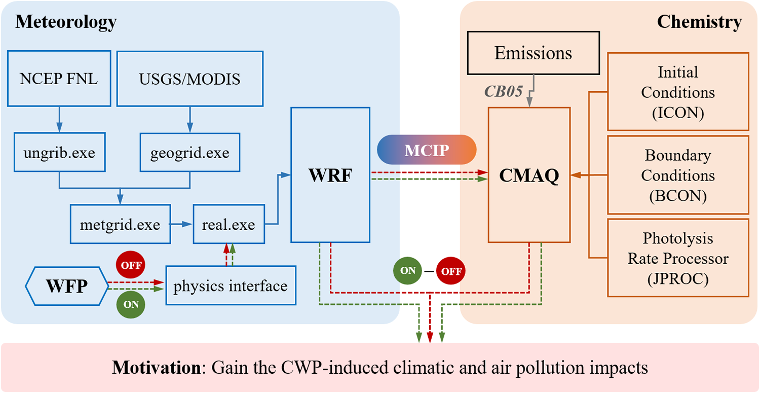
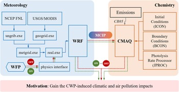
Taking into account the rapid development of wind power in China and the years of severe air quality pollution, we have selected the period from 2009 to 2018 for research and analysis. Among them, the CWP development scenario with a sharp increase in capacity from 26 GW in 2009 to 211 GW in 2018 (Wang et al., Reference Papanastasiou, Melas and Lissaridis2019), during which the central and eastern regions suffered severe haze events, especially air quality reached its peak in December 2013 (Zhang et al., Reference Zhang, He and Huo2019), resulted in daily average PM2.5 concentrations exceeding 150 μg · m−3, and in some areas even reaching 300 to 500 μg · m−3. Accordingly, this 10-year scenario provides a realistic representation of the explosive development of CWP and the serious air quality issues in China. The wind power scenario is established based on data from the Chinese Wind Energy Association. Considering the significant continental monsoon climate in China (Y. Wang et al., Reference Wang, Luo, Yuan, Zhang and Fan2015), we conduct simulations for winter (from December to February, WIN) and summer (from June to August, SUM) for each year from 2009 to 2018. For each phase, the control simulations are conducted both with wind farms (WF) and without wind farms (NWF), which consider the impact of coal-fired power plants on the atmospheric environment. The climatic and air pollution impacts of CWP are represented by the difference Δ between the atmospheric processes driven by the WF and NWF cases. In the present study, the atmospheric processes are simulated by the WRF-CMAQ modeling system (Byun & Schere, Reference Byun and Schere2006; Skamarock et al., Reference Saidur, Rahim, Islam and Solangi2008), in which the CMAQ model is used to simulate the atmospheric chemistry, the WRF model is used to generate the meteorological fields, and the one-way online connection is realized by using the Meteorology-Chemistry Interface Processor (MCIP) (Otte & Pleim, Reference Mlawer, Taubman, Brown, Iacono and Clough2010). The wind farm parameterization (WFP) (Fitch, Olson, et al., Reference Fitch, Olson and Lundquist2013) is used to describe the influence of a wind turbine on the atmosphere. Thereby, the combined modeling system WRF-WFP-CMAQ is established, and the flow charts of WRF and CMAQ are illustrated as shown in Figure 2. The grid resolution is designed according to the suggestion proposed by the previous studies (Mangara et al., Reference Lundquist, DuVivier, Kaffine and Tomaszewski2018; Tomaszewski & Lundquist, Reference Sun, Luo, Zhao and Chang2020) to properly capture the wind farm wakes in the WRF-WFP model. In these simulations, we update the WFP by using the thrust, power, and TKE coefficients from three representative turbines during three different stages, namely, 2009–2011, 2012–2014, and 2015–2018.
The flow chart of the combined modeling system of WRF-WFP-CMAQ in the present study.
2.3. WRF model and simulation setup
Meteorological processes are simulated by using WRF model version 3.7.1 (Skamarock et al., Reference Saidur, Rahim, Islam and Solangi2008), which solves the fully compressible and Euler non-hydrostatic problem with a run-time hydrostatic option equation based on terrain-following hydrostatic pressure coordinates. The WRF model primarily employs the finite-difference technique to discretize the governing equations, which describe atmospheric flows and thermodynamics (Skamarock et al., Reference Saidur, Rahim, Islam and Solangi2008). Moreover, the Advanced Research WRF (ARW) dynamical core is implemented, which uses a third-order Runge–Kutta time-stepping scheme combined with a fifth-order upstream-downwind advection algorithm for horizontal advection. For vertical advection, it adopts a mass-flux scheme to ensure conservation properties. The equations of the forces stemming from model physics (FU), turbulent mixing (FV), spherical projections (FW), and the Earth's rotation (F Θ) are formulated in flux forms, as expressed below, enabling the development of a conserved difference scheme and the elucidation of energy conversion relations within the atmosphere.
 \begin{equation}\left\{ \begin{gathered}
{\partial _t}U + (\nabla \cdot {\textbf{U}}u) + {\mu _d}\alpha {\partial _x}p + (\alpha /{\alpha _d}){\partial _\eta }p{\partial _x}\phi = {F_U} \hfill \\
{\partial _t}V + (\nabla \cdot {\textbf{U}}v) + {\mu _d}\alpha {\partial _y}p + (\alpha /{\alpha _d}){\partial _\eta }p{\partial _y}\phi = {F_V} \hfill \\
{\partial _t}W + (\nabla \cdot {\textbf{U}}w) - g[(\alpha /{\alpha _d}){\partial _\eta }p - {\mu _d}] = {F_W} \hfill \\
{\partial _t}\Theta + (\nabla \cdot {\textbf{U}}\theta ) = {F_\Theta } \hfill \\
{\partial _t}{Q_m} + (\nabla \cdot {\textbf{U}}{q_m}) = {F_{{Q_m}}} \hfill \\
\end{gathered} \right.\end{equation}
\begin{equation}\left\{ \begin{gathered}
{\partial _t}U + (\nabla \cdot {\textbf{U}}u) + {\mu _d}\alpha {\partial _x}p + (\alpha /{\alpha _d}){\partial _\eta }p{\partial _x}\phi = {F_U} \hfill \\
{\partial _t}V + (\nabla \cdot {\textbf{U}}v) + {\mu _d}\alpha {\partial _y}p + (\alpha /{\alpha _d}){\partial _\eta }p{\partial _y}\phi = {F_V} \hfill \\
{\partial _t}W + (\nabla \cdot {\textbf{U}}w) - g[(\alpha /{\alpha _d}){\partial _\eta }p - {\mu _d}] = {F_W} \hfill \\
{\partial _t}\Theta + (\nabla \cdot {\textbf{U}}\theta ) = {F_\Theta } \hfill \\
{\partial _t}{Q_m} + (\nabla \cdot {\textbf{U}}{q_m}) = {F_{{Q_m}}} \hfill \\
\end{gathered} \right.\end{equation} where μd is the dry air mass, p is the hydrostatic pressure, and ϕ is the geopotential. α = αd(1 +∑qi)−1 is the inverse density, and αd is the inverse density. Here, Qm = μdqm, where qm is the mixing ratio. The dry inverse density diagnostic equation is  ${\partial _\eta }$ = −αdμd. The variables in flux form are formulated as follows because μ(x, y) represents the mass per unit area at (x, y):
 \begin{equation}\left\{ \begin{gathered}
{\textbf{U}} = {\mu _d} {\textbf{u}} = \left( {U,V,W} \right) \hfill \\
\Omega = {\mu _d}\omega \hfill \\
\Theta = {\mu _d}\theta \hfill \\
\end{gathered} \right.\end{equation}
\begin{equation}\left\{ \begin{gathered}
{\textbf{U}} = {\mu _d} {\textbf{u}} = \left( {U,V,W} \right) \hfill \\
\Omega = {\mu _d}\omega \hfill \\
\Theta = {\mu _d}\theta \hfill \\
\end{gathered} \right.\end{equation}where u = (u, v, w) are the horizontal and vertical covariant velocities; ω is the contravariant vertical velocity; and θ is the potential temperature.
The meteorological boundary and initial conditions are sourced from the Final Operational Global Analysis dataset with a 1° × 1° grid resolution from the National Centers for Environmental Prediction (Saha et al., Reference Ruan, Lu, Wang, Xing, Wang, Chen, Nielsen, Luo, He and Hao2011). To reduce meteorological deviations, the grid-budging approach is used for four-dimensional data assimilation (FDDA) (F. Zhang et al., Reference Yu, Wang, Gao and Sun2015). A Lambert projection with two true latitudes of 25 °N and 40 °N is used for a single domain covering the inland and offshore regions of China, extending from 82.3 °E to 137.7 °E and from 7.3 °N to 50.7 °N, as shown in Figure 1. The model uses Arakawa C-grid staggering for the horizontal grid with 712 × 550 cells at a fine horizontal resolution of 9 km × 9 km. To resolve the atmospheric processes in the atmospheric boundary layer (Li et al., Reference Li, Zhang, Cai, Song and Zhu2021), the vertical resolution is designed to be ∼8.7 m in the lowest 160 m, stretching vertically thereafter, and 45 eta levels are used in total, as illustrated in Fig. S1. This vertical grid system intersects the turbine rotor with 7, 10, and 14 layers respectively for the three representative wind turbines at the three phases. It meets the requirement of vertical resolution (∼10 m) suggested by (Mangara et al., Reference Lundquist, DuVivier, Kaffine and Tomaszewski2018) and (Tomaszewski & Lundquist, Reference Sun, Luo, Zhao and Chang2020). Time-split integration is performed by using a 3rd-order Runge–Kutta scheme with a time step of approximately 10 s for gravity-wave modes. The geographical data are derived from the Moderate Resolution Imaging Spectroradiometer (MODIS)-based land use data. In addition, the following physics schemes are used for physical processes: the simple microphysical process is parameterized by the WRF Single-Moment Six-Class (WSM-6) microphysics scheme (Hong, Reference Hong2006), longwave radiation and shortwave radiation is represented by an accurate rapid radiative transfer model (RRTM) (Mlawer et al., Reference Miller and Keith1997) and the Goddard radiation scheme (Fouquart et al., Reference Fouquart, Bonnel and Ramaswamy1991), respectively, and the land surface physics is parameterized by the Noah land surface model (Ek et al., Reference Ek, Mitchell, Lin, Rogers, Grunmann, Koren, Gayno and Tarpley2003). The Mellor-Yamada-Nakanishi-Niino Level 2.5 (MYNN2) (Fitch et al., Reference Fitch, Olson, Lundquist, Dudhia, Gupta, Michalakes and Barstad2012; Xia et al., Reference Wyoming2017) planetary boundary layer (PBL) physics scheme is utilized with the Grell–Devenyi ensemble cumulus parameterization (Yu et al., Reference Yan, Shi, Chen, Wang, Mao and Liu2011) to ensure the proper implementation of the wind farm parameterization (WFP). The WRF model coupled with and without the WFP is used to simulate meteorological processes with and without wind farms in China, respectively; thus, the CWP-induced climatic and air pollution impacts could be represented by the difference between the atmospheric processes driven by the cases with and without the WFP.
2.4. Wind farm parameterization
In the WRF model, the high-frequency variability of the wind-turbine interaction can be resolved by using the WFP initially developed by Fitch, Lundquist, et al., (Reference Fitch, Lundquist and Olson2013) and Fitch et al., (Reference Fitch, Olson, Lundquist, Dudhia, Gupta, Michalakes and Barstad2012). The WFP interacts with the PBL scheme (MYNN2) by adding a turbulence source and a momentum sink to the governing equations within the vertical levels of the turbine rotors in the simulations (Keith et al., Reference Keith, DeCarolis, Denkenberger, Lenschow, Malyshev, Pacala and Rasch2004). The kinetic energy extracted from the atmosphere by wind turbines is computed by the thrust coefficient, which depends on the wind speed and is converted into electrical energy as a function of the power coefficient; the rest is converted into turbulent kinetic energy. In the grid (i, j, k), the rate of kinetic energy (KE) loss resulting from the disturbance caused by the wind turbine can be expressed as:
 \begin{equation}\frac{{\partial {\text{KE}}_{{\text{drag}}}^{ijk}}}{{\partial t}} = - \frac{1}{2}N_t^{}\Delta x\Delta y{C_T}{\rho _{ijk}}\left| {\textbf{U}} \right|_{ijk}^3{A_{ijk}}\end{equation}
where Nt is the wind turbine number in each grid, Δx and Δy are the spatial resolutions in the latitude and longitude directions, and Aijk is the cross-section area cut by the rotor between the levels k and k + 1. Given the significance of the horizontal velocity component relative to the vertical velocity, the rate of change in KE within the ABL and confined to the grid cell (i, j) can be mathematically expressed as follows:
 \begin{equation}\frac{{\partial {\text{KE}}_{{\text{cell}}}^{ijk}}}{{\partial t}} = {\rho _{ijk}}{\left| {\textbf{U}} \right|_{ijk}}\frac{{\partial {{\left| {\textbf{U}} \right|}_{ijk}}}}{{\partial t}}\left( {{z_{k + 1}} - {z_k}} \right)\Delta x\Delta y\end{equation}
Based on the principle of energy conservation, the rate of change in KE within the ABL is equivalent to the KE loss rate induced by the turbine in each grid cell, and the momentum tendency term is:
 \begin{equation}\frac{{\partial {{\left| {\textbf{U}} \right|}_{ijk}}}}{{\partial t}} = - \frac{1}{2}\frac{{N_T^{ij}{C_T}\left| {\textbf{U}} \right|_{ijk}^2{A_{ijk}}}}{{\left( {{z_{k + 1}} - {z_k}} \right)}}\end{equation}
The energy extracted from the atmosphere undergoes a conversion process into electrical energy (P) and turbulent kinetic energy (TKE) dissipated within the atmosphere, which are determined using the following calculations:
 \begin{equation}\left\{ \begin{gathered}
\frac{{\partial {P_{ijk}}}}{{\partial t}} = \frac{1}{2}\frac{{N_T^{ij}{C_p}\left| {\textbf{U}} \right|_{ijk}^3{A_{ijk}}}}{{\left( {{z_{k + 1}} - {z_k}} \right)}} \hfill \\
\frac{{\partial {\text{TK}}{{\text{E}}_{ijk}}}}{{\partial t}} = \frac{1}{2}\frac{{N_T^{ij}{C_{{\text{TKE}}}}\left| {\textbf{U}} \right|_{ijk}^3{A_{ijk}}}}{{\left( {{z_{k + 1}} - {z_k}} \right)}} \hfill \\
\end{gathered} \right.\end{equation}
\begin{equation}\left\{ \begin{gathered}
\frac{{\partial {P_{ijk}}}}{{\partial t}} = \frac{1}{2}\frac{{N_T^{ij}{C_p}\left| {\textbf{U}} \right|_{ijk}^3{A_{ijk}}}}{{\left( {{z_{k + 1}} - {z_k}} \right)}} \hfill \\
\frac{{\partial {\text{TK}}{{\text{E}}_{ijk}}}}{{\partial t}} = \frac{1}{2}\frac{{N_T^{ij}{C_{{\text{TKE}}}}\left| {\textbf{U}} \right|_{ijk}^3{A_{ijk}}}}{{\left( {{z_{k + 1}} - {z_k}} \right)}} \hfill \\
\end{gathered} \right.\end{equation}where zk +1 and zk represent the bellow and top-level heights of the grid cell with the vertical index of k in the model.
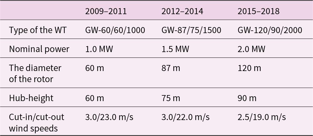
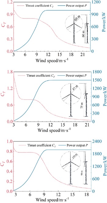
In this model, the wake effect is slightly underestimated due to the unresolved flow around the wind turbine in a grid larger than the distance between two turbines, but many previous studies (Baidya Roy & Traiteur, Reference Baidya Roy and Traiteur2010; Fitch et al., Reference Fitch, Olson, Lundquist, Dudhia, Gupta, Michalakes and Barstad2012; Miller & Keith, Reference Mangara, Guo and Li2018; Sun et al., Reference Su, Li and Kahn2018; Vautard et al., Reference Tomaszewski and Lundquist2014) have demonstrated that this model can reasonably represent the interaction between wind farms and the atmosphere. In the present study, we update the WFP by using local geographical data, the equivalent nominal power, and corresponding lists of thrust and power versus the wind speed from cut-in to cut-out for the typical wind turbines in three different phases, namely, GW-60/60/1000 (the diameter in meters/hub height in meters/nominal power in kilowatts) in 2009–2011, GW-87/75/1500 in 2012–2014, and GW-120/90/2000 in 2015–2018. The detailed parameters are listed in Figure 3 and Table 1. During the WRF-WFP simulations, the time step is 10 s. The results can be output every hour and averaged over a certain period to obtain temporally averaged data.
The wind turbine thrust coefficient and power output curves in each phase.
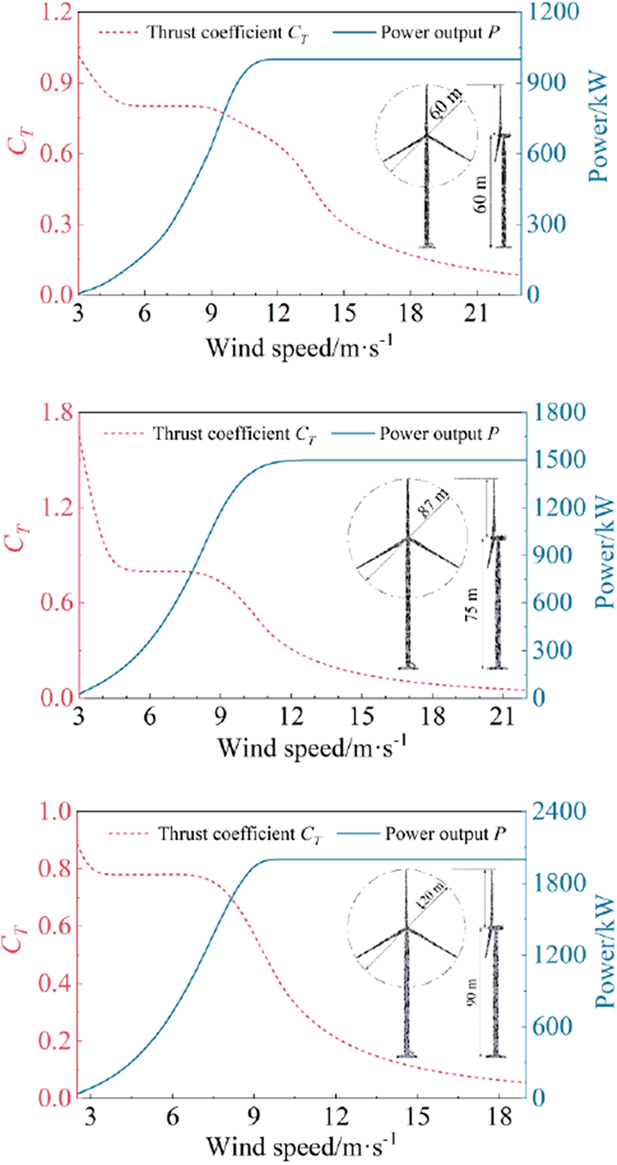
The basic parameters of the typical wind turbines used in the WFP model in each phase of the multiyear simulations
2.5. CMAQ model and simulation setup
The hemispheric version of the CMAQ (Byun & Schere, Reference Byun and Schere2006) modeling system (www.epa.gov/cmaq) is used to simulate air pollution with the meteorological fields generated by the Meteorology Chemistry Interface Processor (Otte & Pleim, Reference Mlawer, Taubman, Brown, Iacono and Clough2010) (MCIP version 4.3) using the outputs from the WRF model introduced above. The CMAQ model primarily adopts the finite-volume method for solving the equations that govern atmospheric chemistry (Byun & Schere, Reference Byun and Schere2006). This method ensures the conservation of mass, momentum, and species concentrations by integrating the equations over control volumes. Moreover, the chemical transformations and transport processes are typically solved using an iterative solver, combined with a sparse matrix solver for efficiency. The model also incorporates advanced advection schemes to handle tracer transport accurately. The CMAQ model is an Eulerian photochemical air quality model in which complex interactions between atmospheric pollutants on urban, regional, and hemispheric scales are treated in a consistent framework. Based on the correlation principle between the generalized meteorological vertical coordinate system and the rotating spherical coordinate system, the expression for the three-dimensional Euler control equation of pollutant concentration in the Chemical Transport Module (CCTM) can be expressed as:
 \begin{equation}
\begin{array}{@{}l@{}}
\dfrac{{\partial \varphi _i^*}}{{\partial t}} + {\nabla _\xi } \cdot \left[ {\varphi _i^*{{\bar{\mathbf{ U}}}_\xi }} \right] + \dfrac{{\partial (\varphi _i^*\overline {{u^3}} )}}{{\partial {x^3}}} + {\nabla _\xi } \cdot \left[ {\bar \rho \sqrt \gamma {{\mathbf{F}}_{{q_i}}}} \right] \\[5pt]
\ (\text{a})\quad\qquad (\text{b})\qquad\qquad\ \ (\text{c})\qquad\qquad\quad (\text{d}) \\[5pt]
\qquad +\, \dfrac{{\partial (\bar \rho \sqrt \gamma {\mathbf{F}}_{{q_i}}^3)}}{{\partial {x^3}}} = \sqrt \gamma {R_{{\varphi _i}}}({{\bar \varphi }_i}, \ldots ,{{\bar \varphi }_N}) + \sqrt \gamma {S_{{\varphi _i}}} \\[5pt]
\qquad\qquad\quad\, (\text{e})\qquad\quad \quad\qquad\quad\ (\text{f})\qquad\qquad (\text{g}) \\[5pt]
\qquad +\, {\left. {\dfrac{{\partial (\varphi _i^*)}}{{\partial t}}} \right|_{{\text{cloud}}}} + {\left. {\dfrac{{\partial (\varphi _i^*)}}{{\partial t}}} \right|_{{\text{ping}}}} + {\left. {\dfrac{{\partial (\varphi _i^*)}}{{\partial t}}} \right|_{{\text{areo}}}} \\[5pt]
\qquad\qquad\ \ \,(\text{h}) \quad\qquad\ \ (\text{i})\qquad\qquad\ (\text{j})
\end{array}
\end{equation}
\begin{equation}
\begin{array}{@{}l@{}}
\dfrac{{\partial \varphi _i^*}}{{\partial t}} + {\nabla _\xi } \cdot \left[ {\varphi _i^*{{\bar{\mathbf{ U}}}_\xi }} \right] + \dfrac{{\partial (\varphi _i^*\overline {{u^3}} )}}{{\partial {x^3}}} + {\nabla _\xi } \cdot \left[ {\bar \rho \sqrt \gamma {{\mathbf{F}}_{{q_i}}}} \right] \\[5pt]
\ (\text{a})\quad\qquad (\text{b})\qquad\qquad\ \ (\text{c})\qquad\qquad\quad (\text{d}) \\[5pt]
\qquad +\, \dfrac{{\partial (\bar \rho \sqrt \gamma {\mathbf{F}}_{{q_i}}^3)}}{{\partial {x^3}}} = \sqrt \gamma {R_{{\varphi _i}}}({{\bar \varphi }_i}, \ldots ,{{\bar \varphi }_N}) + \sqrt \gamma {S_{{\varphi _i}}} \\[5pt]
\qquad\qquad\quad\, (\text{e})\qquad\quad \quad\qquad\quad\ (\text{f})\qquad\qquad (\text{g}) \\[5pt]
\qquad +\, {\left. {\dfrac{{\partial (\varphi _i^*)}}{{\partial t}}} \right|_{{\text{cloud}}}} + {\left. {\dfrac{{\partial (\varphi _i^*)}}{{\partial t}}} \right|_{{\text{ping}}}} + {\left. {\dfrac{{\partial (\varphi _i^*)}}{{\partial t}}} \right|_{{\text{areo}}}} \\[5pt]
\qquad\qquad\ \ \,(\text{h}) \quad\qquad\ \ (\text{i})\qquad\qquad\ (\text{j})
\end{array}
\end{equation} where  $\varphi _i^*{\text{ = }}\sqrt \gamma {\bar \varphi _i} = {{\left| {{{\partial h} \mathord{\left/
{\vphantom {{\partial h} {\partial s}}} \right.
} {\partial s}}} \right|{{\bar \varphi }_i}} \mathord{\left/
{\vphantom {{\left| {{{\partial h} \mathord{\left/
{\vphantom {{\partial h} {\partial s}}} \right.
} {\partial s}}} \right|{{\bar \varphi }_i}} {{m^2}}}} \right.
} {{m^2}}}$, and m represents the map scale factor, h represents the geometric height, s represents the generalized meteorological vertical coordinate; Fqi represents the turbulent flux vector of trace species. The various physical and chemical phenomena: (a) the rate of air pollutant concentration alteration, (b) horizontal convection, (c) vertical convection, (d) horizontal eddy current diffusion transfer, (e) vertical eddy current diffusion transfer, (f) chemical reaction generation, (g) emissions originating from pollution sources, (h) cloud and mist mixing along with liquid phase formation, (i) smoke and rain rise, to (j) aerosol chemical processes. A comprehensive review can be found in the study by Byun and Schere (Reference Byun and Schere2006).
$\varphi _i^*{\text{ = }}\sqrt \gamma {\bar \varphi _i} = {{\left| {{{\partial h} \mathord{\left/
{\vphantom {{\partial h} {\partial s}}} \right.
} {\partial s}}} \right|{{\bar \varphi }_i}} \mathord{\left/
{\vphantom {{\left| {{{\partial h} \mathord{\left/
{\vphantom {{\partial h} {\partial s}}} \right.
} {\partial s}}} \right|{{\bar \varphi }_i}} {{m^2}}}} \right.
} {{m^2}}}$, and m represents the map scale factor, h represents the geometric height, s represents the generalized meteorological vertical coordinate; Fqi represents the turbulent flux vector of trace species. The various physical and chemical phenomena: (a) the rate of air pollutant concentration alteration, (b) horizontal convection, (c) vertical convection, (d) horizontal eddy current diffusion transfer, (e) vertical eddy current diffusion transfer, (f) chemical reaction generation, (g) emissions originating from pollution sources, (h) cloud and mist mixing along with liquid phase formation, (i) smoke and rain rise, to (j) aerosol chemical processes. A comprehensive review can be found in the study by Byun and Schere (Reference Byun and Schere2006).
In the present study, this model is used to investigate the CWP-induced impacts on representative air pollutants, namely, PM2.5 and NO2. The numerical experiments are performed by using CMAQ version 5.0.2 with a domain covering China with 568 × 454 grid cells at a horizontal resolution of 9 km. This domain is contained within the domain of the WRF model, as shown in Figure 1. The vertical grid resolution is the same as the configuration of the WRF model as aforementioned. To minimize the influence of the initial conditions, we implement a 10-day spin-up time before the start day in each case, similar to the WRF simulations. The anthropogenic emissions at a resolution of 9 km are obtained by interpolation from an inventory developed by previous studies (Zhao, Wang, Dong, et al., Reference Zhang, Zheng, Tong, Shao, Wang, Zhang, Xu, Wang, He and Liu2013; Zhao, Wang, Wang, et al., Reference Zhao, Wang, Dong, Wang, Duan, Fu, Hao and Fu2013; Zhao et al., Reference Zhao, Wang, Wang, Fu, Liu, Xu, Fu and Hao2018). Biogenic emissions are generated by the Model of Emissions of Gases and Aerosols from Nature (MEGAN) (Guenther et al., Reference Guenther, Jiang, Heald, Sakulyanontvittaya, Duhl, Emmons and Wang2012). The 2005 Carbon Bond (CB05) gas-phase chemical mechanism and the AERO6 aerosol module are used for atmospheric reactions. The CMAQ model runs with the lateral boundary profiles of the chemical concentration developed for the CB05_AERO6 chemical mechanism, which is designed to represent relatively clean air conditions to exclude the effects from the surrounding regions (Gipson, Reference Gipson1999).
2.6. Model validation
To validate the WRF-CMAQ, the surface meteorological parameters and air pollutants from the simulations are compared with observations from the Wyoming Weather Web (Wyoming, Reference Du, Fang, Huang, Cheng, Dang and Xing2018) and the National Urban Air Quality Real-time Release Platform of the China National Environmental Monitoring Center. The predicted 10 m wind speed (SPD10), 2 m temperature (T2), surface PM2.5, and surface NO2 exhibit reasonable agreement with the observations, indicating the reliability of the current models. Several metrics (Papanastasiou et al., Reference Otte and Pleim2010), such as the mean bias error (MBE), root mean square error (RMSE), and index of agreement (IA), are used to evaluate the performance of the WRF-CMAQ. Firstly, to validate the WRF model, we collect hourly observed surface meteorological data, such as the 2 m temperature (T2) and 10 m wind speed (SPD10), from 32 major cities in China during 2009–2018.
Figure 4 shows the correlations between the simulated SPD10 and T2 and the observations. The simulated results are generally consistent with the observed meteorological factors with the IA values of 0.85 and 0.82 for SPD10 in winter and summer, and 0.97 and 0.86 for T2 in winter and summer, respectively, though it slightly overestimates SPD10 and T2 in summer. Moreover, the spatial correlation comparison with the fifth-generation European Centre for Medium-Range Weather Forecasts Re-Analysis (ERA5) reanalysis dataset obtained from data assimilation was added. The monthly means of several meteorological factors, including the SPD10, T2, and PBLH are evaluated. Figure 5 shows a very similar spatial distribution of T2 between ERA5 and the WRF simulation with a horizontal grid resolution of 9 km, with spatial correlation coefficients of 0.99 in winter and 0.96 in summer, respectively. The SPD10 and PBLH also show a good correlation between the simulations and the ERA5 reanalysis data.
Correlation between the simulated meteorological factors (SPD10 and T2) and the observations.

Comparison of T2 in winter (upper panel) and summer (down panel) between the simulations (left panel) and ERA5 data (right panel) in 2018.

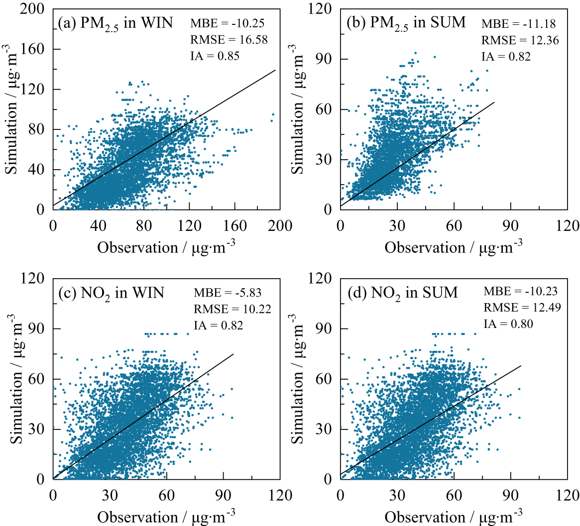
In addition, the hourly observed concentration of air pollutants, namely, surface PM2.5 and NO2, downloaded from the National Urban Air Quality Real-time Release Platform of the China National Environmental Monitoring Center (http://beijingair.sinaapp.com) serves as the benchmark for quantifying the performance of the CMAQ model. The observational data for air pollutants have been updated since May 13, 2014. The number of observation stations was 941 in 2014, 1497 during 2015–2016, and 1569 during 2017–2018, covering most prefecture-level cities in China. The relationships and relevant metrics for the simulated and observed background concentrations of PM2.5 and NO2 are also statistically analyzed, and scatterplots are shown in Figure 6. The MBE values reveal a slight underestimation of air pollutant concentrations, but the IA values for PM2.5 and NO2 are larger than 0.80 for all cases, indicating that the model exhibits good performance when simulating atmospheric chemistry. Therefore, the simulation results are generally consistent with the measured data and can be used to study the climatic and air quality impacts.
Correlation between the simulated air pollutants and the observations.
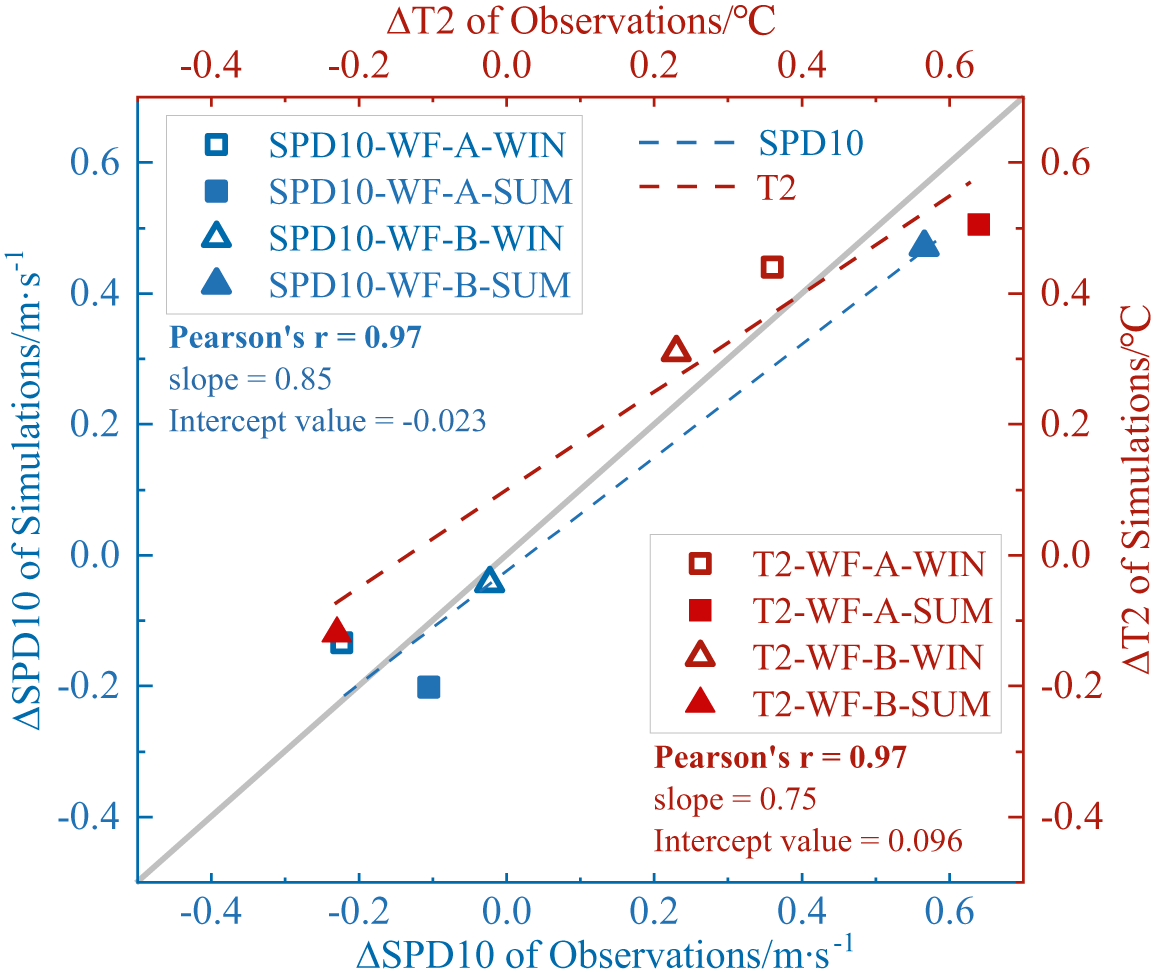
Essentially, a direct comparison of farm-induced climatic impacts between the WRF-CMAQ simulations and the observational data was provided. The available historic (2011–2018) meteorological observations (SPD10 and T2) at two representative weather stations in the BTH and TCM regions (here marked as WF-A in the BTH region and WF-B in the TCM region) were first collected. These historically observed data were then categorized into two groups, i.e., a control group of 2011–2014 during which the limited number of wind farms were operated, and a test group of 2015–2018 during which many new wind farms were installed. The mean modification on SPD10 and T2 due to increased wind farms can be quantified by the difference between the averaged values of the test and control groups. Similarly, the mean modification on SPD10 and T2 due to increased wind farms can also be obtained from the WRF-CMAQ simulations.
Figure 7 shows the comparison of the observed data and simulated results on WF-A in BTH and WF-B in TCM regions in China. The observed changes due to increased wind farms agree well with those of the simulations. This agreement provides strong evidence that the effects induced by wind farms have been well captured by the current simulations. Accordingly, the climatic and air quality impacts induced by CWP are reliable, and the well-validated WRF-CMAQ model can be used for further analysis in the present study.
Comparison of observations and simulations for the locations in the wind farms of WF-A in BTH and WF-B in TCM regions in China. The left and bottom axes stand for the results of SPD10 and the right and top axes stand for the T2.

3. Results
3.1. Seasonal climatic impacts
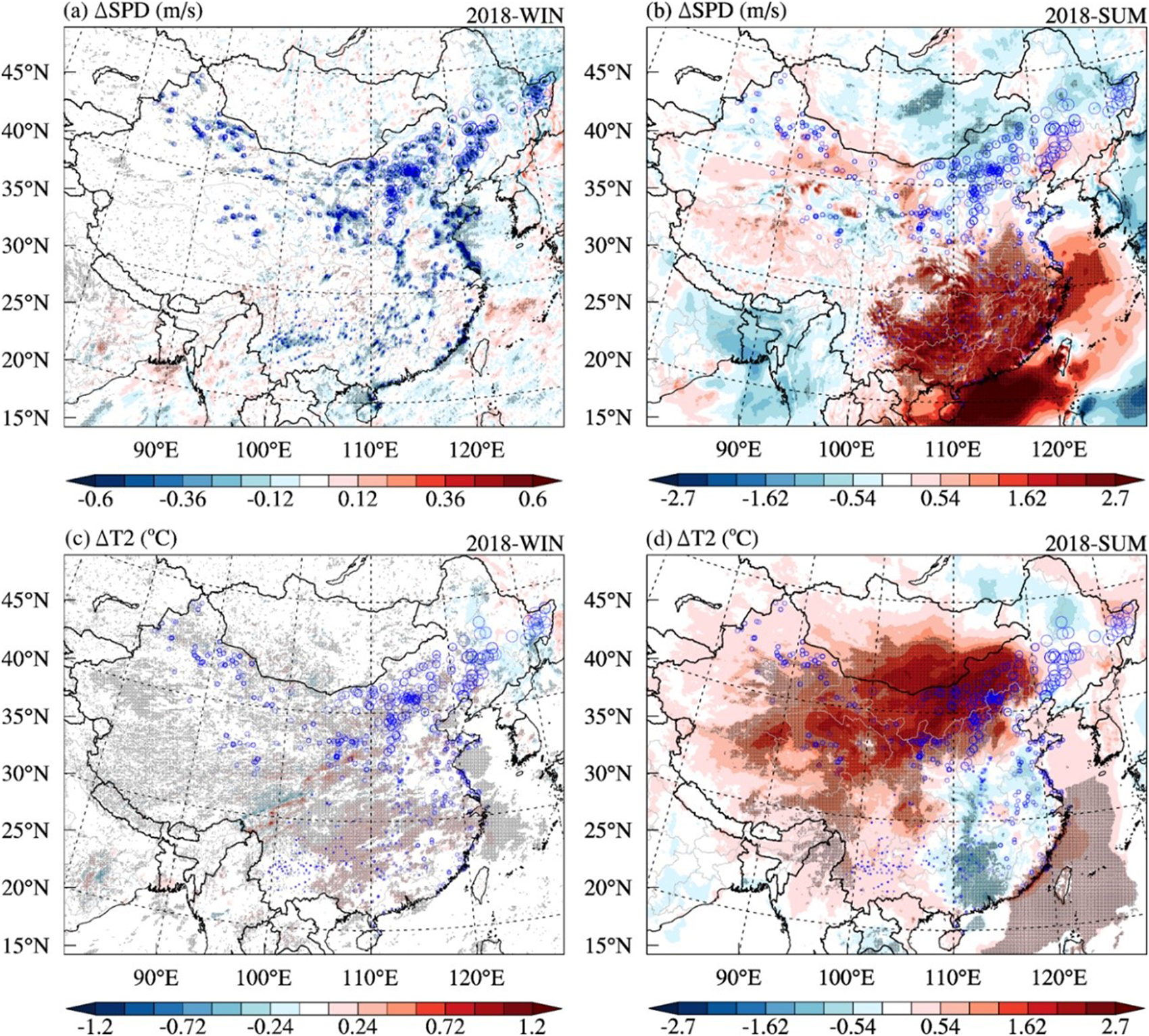
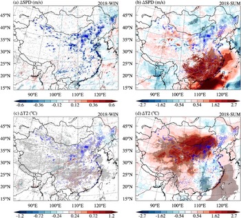
To visualize the CWP-induced seasonal climatic impacts, we illustrate the differences in the hub-height wind speed (ΔSPD) and 2 m temperature (ΔT2) between the WF and NWF cases in 2018, with maximum installed capacity during the period, as illustrated in Figure 8. The hourly SPD and T2 are obtained from the simulations for winter and summer and averaged over the seasons separately to obtain the contours of ΔSPD and ΔT2. In a contrast experiment, a Student's t-test is performed to examine the significance of the changes. It exhibits seasonal variability. In winter, the wind farm region undergoes a maximum wind speed deficit of 4.15 m · s−1 and the largest temperature increase of 1.24 ℃ (Figure 8a, c). This local climatic response is significantly spatially correlated with wind farms due to the immediate wind farm-induced absorption of momentum and TKE generation in the atmosphere in winter (Miller & Keith, Reference Mangara, Guo and Li2018; Wang et al., Reference Papanastasiou, Melas and Lissaridis2019). In contrast, the climatic response shows nonlocal and regional characteristics in summer (Figure 8b, d). Specifically, northern China experiences a remarkable wind loss with a peak of 3.2 m · s−1 and a warming effect with a peak of 2.55 ℃, while southeastern China experiences a seasonal peak wind gain of 4.24 m · s−1 and cooling of 1.43 ℃ and all changes are significant. These significant regional impacts are larger than those reported by some previous studies (Baidya Roy, Reference Baidya Roy2011; Baidya Roy & Traiteur, Reference Baidya Roy and Traiteur2010; Fitch, Reference Fitch2015; Miller & Keith, Reference Mangara, Guo and Li2018; Sun et al., Reference Su, Li and Kahn2018; Xia et al., Reference Xia, Cervarich, Roy, Zhou, Minder, Jimenez and Freedman2015; Zhou et al., Reference Zhao, Li, Zhang, Yang and Liu2012) due to the high capacity of wind power in the study period in China but are comparable to the results from a previous study that employed a general circulation model (Keith et al., Reference Keith, DeCarolis, Denkenberger, Lenschow, Malyshev, Pacala and Rasch2004).
Differences in the hub-height wind speed (ΔSPD) and 2 m temperature (ΔT2) in winter (a, c) and summer (b, d) in 2018. The areas with differences within the 95% confidence interval are indicated by the shaded zones marked with black dots. The blue circles represent wind farms.
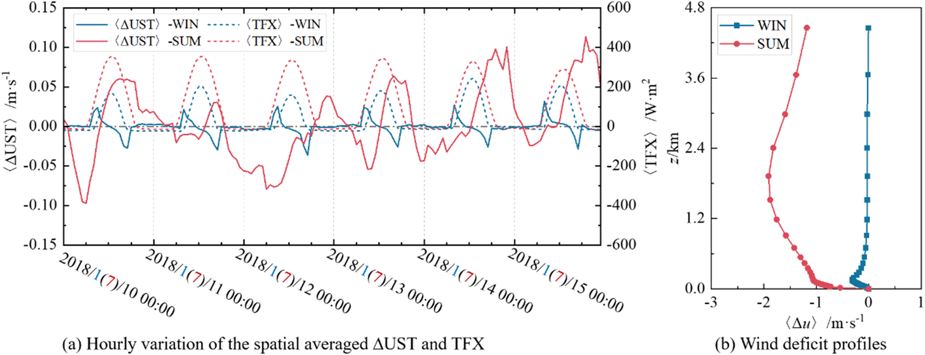
To understand these regional impacts in summer, we trace the CWP-induced surface friction and the background natural turbulent flux. Taking the BTH region as an example, the CWP-induced spatially averaged surface friction speed 〈ΔUST〉, background natural turbulent flux TFX, and wind deficit 〈Δu〉 are presented in Figure 9. Here, 〈TFX〉 represent the atmospheric stability (Miller & Keith, Reference Mangara, Guo and Li2018). The CWP-induced surface friction is small in winter, and the wind deficit is easily recovered below several hundred meters because of the relatively stable atmosphere. In contrast, the CWP-induced surface friction is remarkably large in summer, leading to a larger near-surface wind deficit. This stronger surface impact is easily subject to disturbances and becomes amplified under an unstable atmosphere with a higher TFX, allowing the wind deficit to continue to high levels reaching several kilometers. Indeed, the response of the 500-hPa geopotential height (ΔHGT500) in summer is much larger than that in winter (Fig. S2), indicating that the upper layers are considerably influenced in summer. As a result, a positive ΔHGT500 promotes mesoscale circulation, such as the western Pacific subtropical high surrounding southeastern China, while a negative ΔHGT500 inhibits this circulation, resulting in larger and regional wind gains and warming along the coast and cooling inland (Fig. S3a–c). Another reason might be that the steep vertical temperature gradient in summer is more sensitive to perturbation by wind farms (Miller & Keith, Reference Mangara, Guo and Li2018).
CWP-induced climatic changes in winter and summer in 2018. (a) Hourly variation of the spatially averaged surface friction speed difference 〈ΔUST〉 and background turbulent flux 〈TFX〉. (b) Wind deficit profiles for the BTH region.
3.2. Seasonal air pollution impacts
To investigate how CWP influenced air pollution in 2018, the changes in the concentrations of the representative pollutants of fine particles, namely, PM2.5 and NO2 (Zhang et al., Reference Zhang, Yang and Wang2012), in winter and summer are shown in Figure 10.
Differences in the PM2.5 and NO2 concentrations in winter (a, c) and summer (b, d) in 2018. The data are obtained by averaging the hourly outputs from the simulations in winter and summer. The areas with differences within the 95% confidence interval are indicated by the shaded zones marked with black dots. The blue circles represent wind farms.

In winter, PM2.5 is locally reduced in the wind farm regions but enhanced in the surroundings. However, eastern China is surrounded by significant mesoscale regional changes in summer. PM2.5 increases over northern and northeastern China with a maximum of 13.77 μg · m−3 but decreases in southeastern China with a peak of 16.37 μg · m−3. Similar trends are also found for the redistribution of NO2. During the operation of a wind farm, there are no additional emissions produced, thus, any variations in pollutant levels are primarily attributed to fluctuations in atmospheric conditions. In winter, the PBLH is low, and the turbulence is weak; hence, pollutants tend to accumulate (Su et al., Reference Skamarock, Klemp, Dudhia, Gill, Barker, Duda, Huang, Wang and Powers2018; C. Wang et al., Reference Vautard, Thais, Tobin, Breon, Devezeaux de Lavergne, Colette, Yiou and Ruti2019). Under these conditions, the local atmospheric vertical mixing induced by wind turbines increases the PBLH. This uplift promotes the diffusion of local pollutants into the higher layer and encourages advection to the surrounding regions, thereby increasing pollutant concentrations in the vicinity of wind farms. As a result, a negative correlation between the changes in air pollutants and the ΔPBLH can be observed in the regions with wind farms (Fig. S4a). However, in summer, air pollution usually weakens, while the PBLH rises due to radiative warming, fair vertical mixing, and strong turbulence (Fig. S4b). Accordingly, the CWP-induced pollutant changes show nonlocal and regional features rather than direct correlations with the ΔPBLH and wind farms. This is attributed to the nonlocal regional climatic impacts induced by wind farms in summer. The larger changes in surface meteorological conditions in summer than in winter result in remarkable air pollutant changes, and the relatively unstable atmosphere further promotes these changes through diffusion and advection at a high level, invoking a mesoscale response of air pollutants. Specifically, in northern China, the reduced wind speed strengthens the accumulation of PM2.5, while in southeastern China, the increased wind speed remarkably reduces the concentration of PM2.5 (Fig. S4d).
3.3. Diurnal climatic and air pollutant impacts
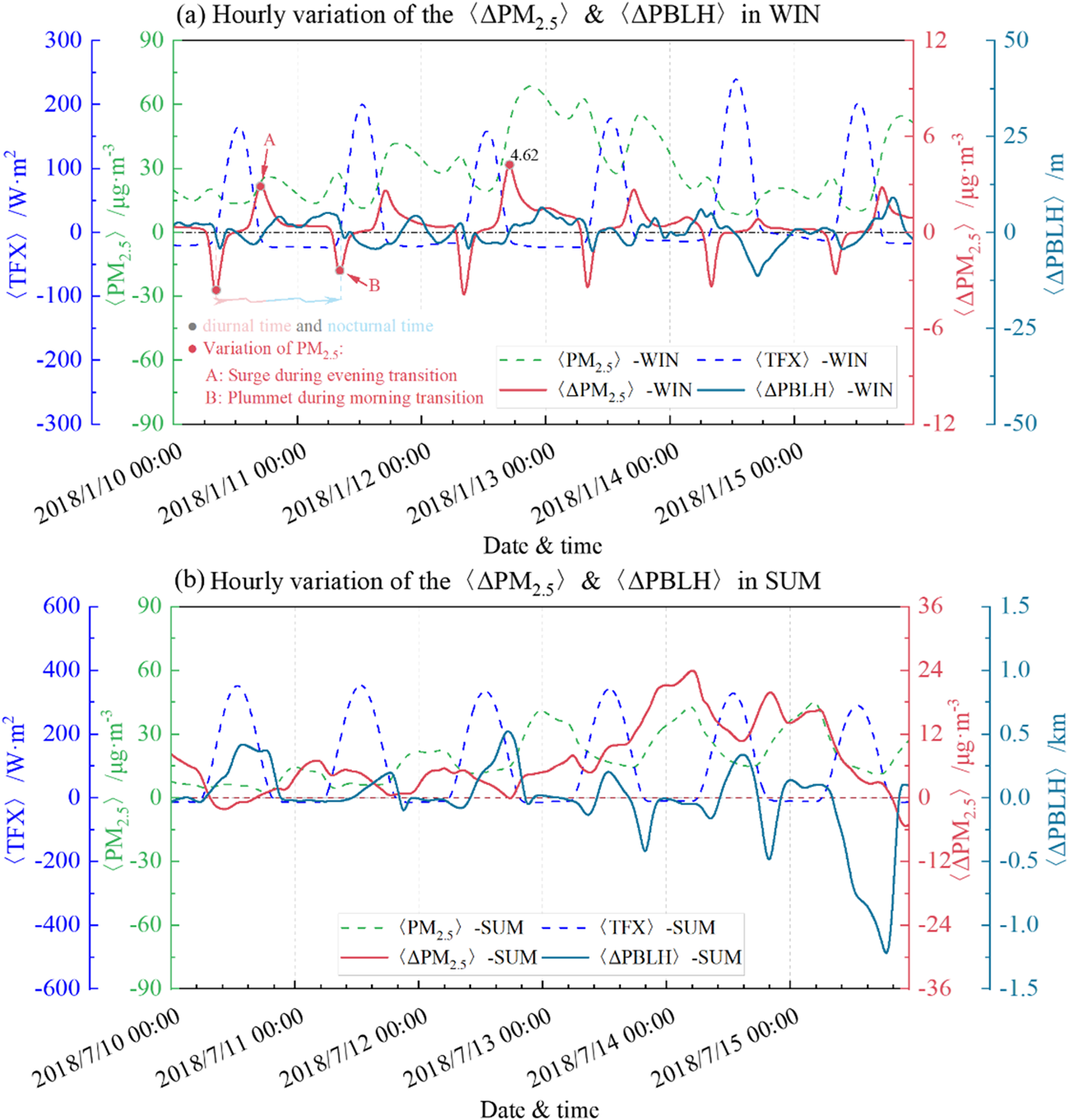
The impact of wind farms on the climate is related to atmospheric stability (Wang, Luo, Ming, et al., Reference Wang, Jia, Xia, Wu, Wei, Shang, Yang, Xue and Dou2023), thus we further explore the critical climate conditions caused by the diurnal variation of atmospheric stability as the daily temperature changes. Here, taking the BTH region as an example, we select six representative day and night cycles in both winter and summer (from January 10 to January 16, 2018, and from July 10 to July 16, 2018) to show the hourly variation patterns of induced meteorological elements, as illustrated in Figure 11.
Diurnal climatic variation in winter and summer in the BTH region: the average turbulence flux 〈TFX〉 and wind speed 〈SPD〉 in the wind farm area, as well as the induced surface friction velocity 〈ΔUST〉 and wind speed 〈ΔSPD〉.
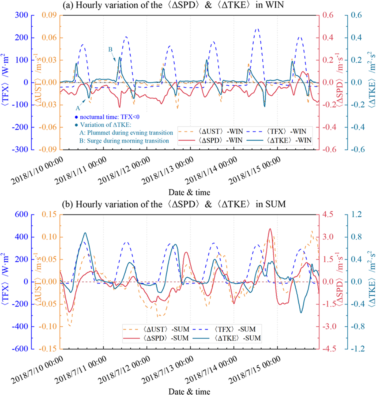
There is a significant diurnal pattern in the climatic elements due to the atmospheric stability as temperature changes. Here we use TFX to reflect the air stability. In winter, the average TFX exhibits pronounced diurnal patterns (Figure 11a). Specifically, the negative signifies a stable layer at night, while, the positive reflects an unstable layer during the day. The average wind in winter remains peaking at 12.5 m · s−1 and emerges a diurnal cycle in the friction velocity. This is evident in a sudden drop in the evening, followed by a marked increase at dawn. Moreover, the wind speed changes are correlated with the TKE changes, which is the main reason for wind loss. However, in summer (Figure 11b), TFX exhibits almost zero at night, indicating a neutral layer, while it has a larger positive during the day, showing an unstable atmosphere. There is no correlation between wind speed changes and turbulence kinetic energy changes.
In addition, the hourly variation of induced air pollutants 〈ΔPM2.5〉 with regional average turbulence flux 〈TFX〉 and atmospheric boundary layer height 〈ΔPBLH〉 are depicted in Figure 12. The alterations in air pollutants triggered by wind farms bear a resemblance to the fluctuations in climate, showing a diurnal cycle pattern. In winter (Figure 12a), the layer is stable at night and the PM2.5 is high, while during the day, the air is unstable and the PM2.5 decreases. Specifically, there is a sharp increase in ΔPM2.5 in the evening and a sudden decrease in ΔPM2.5 at dawn. This is opposite to the trend of wind changes. Meanwhile, the fluctuations in the pollutants display a negative correlation with the alterations in PBLH and wind. In contrast to winter, summer conditions show that wind farms trigger an elevation in PM2.5, devoid of diurnal patterns (Figure 12b). Instead, the changes in ΔPM2.5 align with the fluctuations in background PM2.5 levels, exhibiting a pronounced amplification. Notably, a peak increase of 23.85 μg · m−3 is observed, suggesting a substantial influence of wind farms on air quality in summer. Interestingly, this exhibits a weak negative correlation with variations in the PBLH. This decoupling is attributed to the complex interplay between wind farm operations and atmospheric dynamics in summer.
Diurnal climatic variation in winter and summer in the BTH region: induced air pollutants 〈ΔPM2.5〉 with regional average turbulence flux 〈TFX〉 and atmospheric boundary layer height 〈ΔPBLH〉.
3.4. Long-term impacts
The above results show that CWP had significant local and regional impacts on climate and air pollution in 2018. Here, the multiyear scenarios including three phases, i.e., 2009–2011, 2012–2014, and 2015–2018, with an increasing installed capacity of wind power are evaluated to reflect the long-term trends of the impacts and reduce the uncertainty in the statistics. Figure 13 shows the variations in the ensemble average impacts on the seven megalopolises mentioned above. All parameters are first spatially averaged over each target region and then temporally averaged over the three periods (denoted by “〈〉”).
Variations in the ensemble average impacts on seven megalopolises during three phases: Phase-I: 2009–2011, Phase-II: 2012–2014, and Phase-III: 2015–2018. The horizontal axis denotes the seven regions. All parameters are first spatially averaged over each region and then temporally averaged over each of the three statistical periods, as depicted in the six boxplots. (a) SPD, (b) T2, (c) PM2.5, and (d) NO2. The colors are used to group the data by season: winter (blue, left Y-axis) and summer (red, right Y-axis).
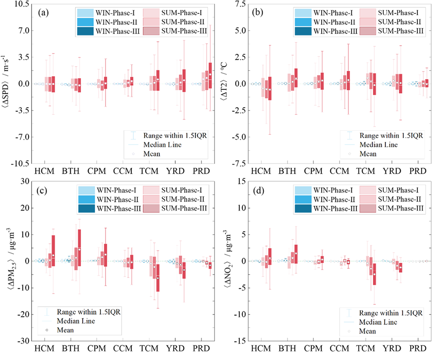
Notably, the CWP-induced impacts on climate and air pollutants become increasingly significant with the increasing installed wind power capacity, and the response in winter is much weaker than that in summer. Almost all areas with dense wind farms experience a slight but rising warming trend and a significant wind deficit in winter, while in summer, the responses show significant regional features (Figure 13a, b). The northern regions, such as BTH and HCM, experience an increase in PM2.5 and a decreased wind speed, while the southern regions, such as the YRD, TCM, and PRD exhibit a decrease in PM2.5 and an enhanced wind speed. Particularly, BTH experienced a remarkable wind loss with a spatial mean of 0.20 m · s−1 and warming with a spatial mean of 0.51 ℃, while YRD experienced a spatial mean wind gain of 0.47 m · s−1 and cooling of −0.12 ℃. These climatic changes are comparable to those in the previous studies about wind farms in China (Hubei Province (Xueting et al., Reference Xia, Zhou, Minder, Fovell and Jimenez2019), Changyi Hebei Province (Liu et al., Reference Liu, Dang, Xu and Weng2021), and entire wind farms in China (Sun et al., Reference Su, Li and Kahn2018)), wind farms in Europe (Vautard et al., Reference Tomaszewski and Lundquist2014), and large-scale wind farms in Continental US (Lundquist et al., Reference Long, Chen, Xu, Li and Wang2018; Miller & Keith, Reference Mangara, Guo and Li2018). The difference in quantitative results is mainly associated with the difference in the scale of wind farms and geographical or meteorological conditions. Moreover, PM2.5 increases in BTH with an average of 4.39 μg · m−3 but decreases in the YRD with an average of −3.27 μg · m−3. According to the study (Zhang et al., Reference Zhang, He and Huo2019), these changes in PM2.5 are equivalent to those achieved by approximately 1 year of the dominant contributions from anthropogenic emission abatements to reduce the national annual mean PM2.5 in China. This finding underscores a potential challenge in the central government's efforts to mitigate PM2.5 pollution, despite investing over 2 billion US dollars annually. Specifically, the potential for impacts in specific regions to undermine these endeavors underscores the intricate challenge of harmonizing clean energy promotion with advancements in air quality.
To further understand the CWP-induced climatic and air pollutant impacts, the hourly ΔSPD and ΔPM2.5 conditioned on the wind and turbulent flux for the multiyear scenarios in the key region of BTH (Zhang et al., Reference Zhang, He and Huo2019) are presented in Figure 14. All values are spatially averaged over the BTH region. In winter, the background wind prevails in the northwest within 3–15 m · s−1, while a wind deficit and an increased PM2.5 concentration emerge between the southwest and southeast with low wind speeds of 3–8 m · s−1 and high temperatures under a relatively stable atmosphere (Figure 14a–c). For all samples, the proportion of the wind speed loss is 86.9%, and the PM2.5 concentration increase is 75.2%, suggesting that the BTH region suffers mainly from wind loss and PM2.5 gain. This outcome is consistent with the results depicted in Figure 13 and might provide evidence to explain the reduction in the wind speed over Beijing from 2.06 m/s in 2009 to 1.84 m/s in 2014 (Du et al., Reference Wu, Luo, Wang and Fan2017). In summer, the background wind is dominant in the southeast within 3–8 m · s−1, and a large number of samples are under an unstable atmosphere (Figure 14d, e). In this situation, the CWP-induced ΔSPD and ΔPM2.5 increase notably, becoming four to five times greater than those in winter (Figure 14c, f).
Conditioned ΔSPD and ΔPM2.5 in the key region of BTH for winter (a–c) and summer (d–f). (a) Each circle in the wind rose represents the hourly wind deficit or gain (the edge color in blue or red, respectively), and the fill color represents the hourly PM2.5 difference in winter. The size and color of the circle are described by the legend in panel (b), which depicts the correlation between ΔSPD, ΔPM2.5, and TFX. The relationships between the spatially averaged hourly ΔSPD, ΔT2, and ΔPM2.5 are plotted in panel (c).

4. Discussion and implications
Our simulations demonstrate that CWP engenders notable climatic and air pollutant impacts in China. Concerning climate, wind farm effects are induced by the immediate absorption of momentum and the generation of TKE. In winter, these impacts are local and limited to the regions surrounding the wind farms, whereas in summer, the induced surface friction is larger and the wind change extends to high levels, modifying the mesoscale circulation. Furthermore, the climatic impacts of CWP redistribute air pollution concentrations. In winter, it shows a reduction in the areas covered by dense wind farms, while an increment in the surroundings. This difference is caused mainly by the ease with which the PBLH is uplifted under a stable atmosphere, as a rise in the PBLH promotes local vertical transport and the advection of pollutants to the surrounding regions. In contrast, in summer, air pollutants exhibit a mesoscale response. These changes in air pollutants are independent of the wind farms due to the mesoscale circulation changes under a strong unstable atmosphere. As a result, in northern China, the reduced wind causes more PM2.5, while in southeastern China, the increased wind reduces the concentration of surface PM2.5. Moreover, it shows the diurnal impacts of wind farms on climatic and air pollutant conditions. Wind farms introduce a diurnal cycle in surface friction velocity, with sharp drops in the evening and an increase at dawn, mirroring similar patterns in induced wind speed. This highlights the importance of considering some critical conditions, such as the diurnal variations, in assessing wind farm impacts on both the climatic impacts and the resultant air pollutant redistribution.
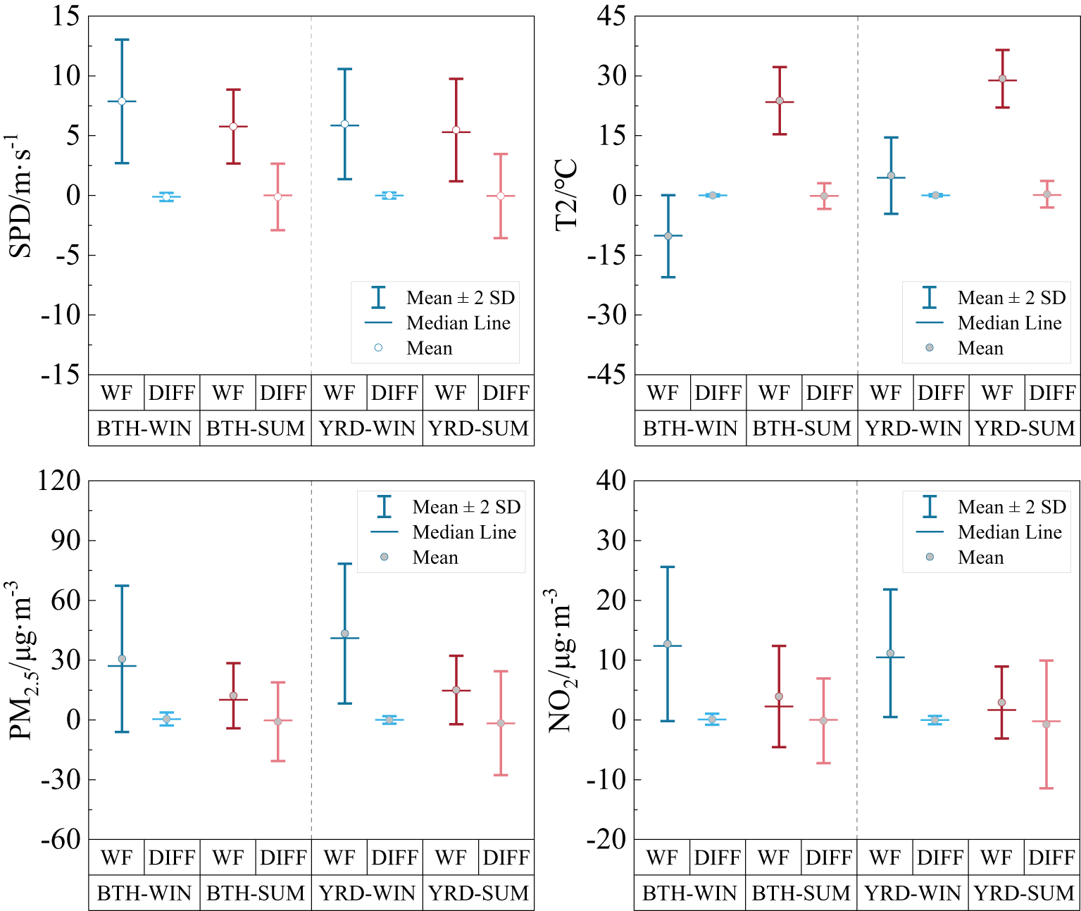
These impacts have become increasingly significant in recent years with the rapidly increasing wind power installation. For instance, in the summer of 2015–2018, the PM2.5 in BTH increased, reaching an average concentration of 4.39 μg · m−3, whereas that in the YRD decreased, with an average concentration of −3.27 μg · m−3. These average changes in PM2.5 are comparable to those obtained by approximately 1 year of dominant contributions from anthropogenic emission abatements to reduce the national annual mean PM2.5 concentrations in China. These results indicate that the impact of wind farms is as likely to be as beneficial as it is harmful. Generally, wind farms do not produce additional emissions, but redistribute air pollutants. The redistribution of air pollutants by wind farms may impose additional difficulties on air pollution control and cause climate, economic, societal, policy, and legal issues (Lundquist et al., Reference Long, Chen, Xu, Li and Wang2018). Statistics also show that the CWP-induced impacts in summer are approximately five times greater than those in winter, and are comparable to inter-annual variability in summer (Figure 15), again confirming that wind farms have significant regional climatic and air pollutant impacts in summer. Therefore, a comprehensive evaluation system and environmentally friendly assessment methods of the environmental impacts caused by wind power are urgent to be established. Furthermore, the government should pay more attention to balancing the development of wind power in different regions and assess or predict the regional impacts of the established and planned wind farms on the ecological environment and climate change via the established evaluation system and assessment methods that cater to the healthy development of the wind power industry.
Spatial average daily parameters with twice the standard deviation in winter and summer (dark blue and red segments in the WF columns) for the regions of BTH and YRD: SPD (a), T2 (b), PM2.5 (c), and NO2 (d). Spatial average daily changes induced by CWP in corresponding regions and periods (light blue and red segments in the DIFF columns).

Supplementary material
The supplementary material for this article can be found at https://doi.org/10.1017/sus.2025.19.
Acknowledgements
The authors would like to thank the anonymous reviewers for their constructive comments and suggestions for improvement. Useful suggestions and CMAQ simulations provided by Dr. Qiang Zhang, Guannan Geng, and Shigan Liu of Tsinghua University are also acknowledged. Numerical computations were performed at Hefei Advanced Computing Center.
Author contributions
Qiang Wang: conceptualization, data curation, formal analysis, funding acquisition, investigation, methodology, resources, software, validation, visualization, writing – original draft, writing – review & editing. Kun Luo: conceptualization, formal analysis, funding acquisition, project administration, supervision, writing – original draft, writing – review & editing. Qing Wang: software, validation, visualization. Jianren Fan: supervision.
Funding statement
This work was supported by the Fundamental Research Funds for the Central Universities (grant number 226-2024-00017), the National Natural Science Foundation of China (grant number 52,206,281), the Zhejiang Provincial Natural Science Foundation of China (grant number LY24E060002), and the State Key Laboratory of Clean Energy Utilization Fund Project (grant number ZJUCEU2023005).
Competing interests
The authors declare that they have no conflicts in this paper.
Research Transparency and Reproducibility
Data will be made available on request


 Open access