

Introduction
Despite the ever-increasing attention on research on DNA and cellulose (exemplified, for instance, by the works of Kostag et al. (Reference Kostag, Jedvert, Achtel, Heinze and El Seoud2018, Reference Kostag, Gericke, Heinze and El Seoud2019), Budtova and Navard (Reference Budtova and Navard2016), Chen et al. (Reference Chen, Zhang, You and Xu2019), Podgornik et al. (Reference Podgornik, Aksoyoglu, Yasar, Svenšek and Parsegian2016), Travers and Muskhelishvili (Reference Travers and Muskhelishvili2015), Frank-Kamenetskii and Prakash (Reference Frank-Kamenetskii and Prakash2014) or Peters and Maher (Reference Peters and Maher2010) dictated by the genetic role and the role as a raw material in achieving a more sustainable society, respectively, aspects related to basic mechanisms continue to be controversial. In particular, the recent attempts to understand the balance between hydrophilic and hydrophobic properties are noted (Glasser et al., Reference Glasser, Atalla, Blackwell, Malcolm Brown, Burchard, French, Klemm and Nishiyama2012; Vologodskii and Frank-Kamenetskii, Reference VologodskII and Frank-Kamenetskii2018; Feng et al., Reference Feng, Sosa, Mårtensson, Jiang, Tong, Dorfman, Takahashi, Lincoln, Bustamante, Westerlund and Nordén2019).
For DNA, the self-assembly into the double helix is a most significant feature whereas for cellulose, since it cannot be processed via melting, dissolution in aqueous media is a central issue. As will be discussed in this review, an understanding relates to the balance between hydrogen bonding and hydrophobic interactions. Recent research has demonstrated that often the hydrophobic interactions have been underestimated. Both DNA and cellulose have parts that are distinctly nonpolar, and to understand the behaviour of these macromolecules in an aqueous environment, they must be treated as amphiphilic (Fig. 1).
Amphiphilic nature of DNA, cellulose and surfactants.

For many situations where hydrophobic interactions are the driving force, hydrogen bonds are simultaneously established. Whereas hydrogen bonds do not drive association in an aqueous medium, they may occur as molecules are transferred to a less polar environment; in nonpolar solvents, hydrogen bonding is an important driving force for the association. An illustrative example is benzoic acid; in water association by hydrogen bonding does not occur, but as it is transferred to a nonpolar environment dimerization is induced due to hydrogen bonding (Nordén, Reference Nordén1977). For more amphiphilic molecules there are numerous cases where self-assembly due to hydrophobic interactions create nonpolar regions and drive hydrogen bonding to occur. One example is the peculiar behaviour of acid soaps in water (Ekwall, Reference Ekwall1937). Here, hydrogen bonding between fatty acid molecules and soap anions accompanies a hydrophobically driven self-assembly. Another case is that of surfactants with amide groups; in this case, hydrogen bonding is induced on micelle formation but does not occur at concentrations below the critical micelle concentration. Similarly, hydrogen bonding is induced between the amide surfactant molecules at the air−water interface and has a large impact on foam stability (Stubenrauch et al., Reference Stubenrauch, Hamann, Preisig, Chauhan and Bordes2017; Preisig et al., Reference Preisig, Schad, Jacomine, Bordes and Stubenrauch2019; Kanduč et al., Reference Kanduč, Schneck and Stubenrauch2021). That the same considerations apply for DNA and cellulose has frequently been overlooked. As will be discussed in this review, two strands of DNA associate due to hydrophobic interactions, the process not being driven by hydrogen bonding. In the nonpolar interior of the double helix, hydrogen bonding is naturally established and provides the specificity in base-pairing. In both native and regenerated cellulose, there are strong hydrophobic interactions between cellulose molecules; in the nonpolar environment created on the association, hydrogen bonds between cellulose molecules are formed but again they are not driving the association. Since for DNA and cellulose hydrogen bonds with water are as strong as solute−solute hydrogen bonds, hydrogen bonding cannot be the driving force for the association.
Surfactant and polar lipid micellization and other types of self-assembly are probably the most clear-cut and deeply studied aspects of intermolecular interactions due to hydrophobic interactions. As we will see, some important points of association in DNA and cellulose systems have their parallels in surfactant self-assembly; in particular, we will note here the role of electrostatic interactions due to net charges and the effect of polar additives on the hydrophobic interactions. Sodium dodecyl sulphate, as the most studied surfactant, is taken as an example. As a result of electrostatic repulsions between the sulphate head-groups, notably counterion entropy effects, self-assembly is relatively weak, with a high critical micelle concentration (CMC) compared to non-ionic surfactants. On screening the electrostatic repulsions, by adding salt, or an oppositely charged amphiphilic substance, the association becomes much stronger. This has parallels for both DNA and cellulose. Thus, the DNA double helix is less prone to form in the absence of electrolyte; its formation is stabilized by the addition of salt as well as many cationic co-solutes, including surfactants. Cellulose dissolution in water only occurs if cellulose is charged-up, either by protonation or by deprotonation; amphiphilic cosolutes can strongly affect solubility and regeneration and the same applies to electrolytes.
Polar additives, such as urea, dioxane and polyethylene glycol markedly reduce the tendency of surfactant self-assembly, as can be learnt from a huge literature on additive effects on CMC. Interestingly, completely analogous effects are seen of such cosolutes in base stacking in DNA and cellulose dissolution.
Since we feel a need to clarify the balance between different interactions in DNA and cellulose systems we here present an overview of pertinent observations. In particular, we argue that the role of hydrogen bonding has often been overemphasized with respect to hydrophobic interactions. Whereas this review will deal only with DNA and cellulose, it is our contention that similar analyses would be valuable for many other biological and synthetic macromolecules.
Amphiphilic molecules and the hydrophobic effect
DNA and cellulose are macromolecules of widely different character. Still, we will see that very much the same aspects apply regarding amphiphilicity and the balance between hydrophobic and hydrophilic interactions. Amphiphilic compounds, i.e. those which have distinct hydrophilic and lipophilic parts, are used in most branches of industry and are ubiquitous in biological systems. They range from low molecular weight substances, like surfactants and lipids, to macromolecules, comprising synthetic graft and block copolymers, and biomacromolecules, such as proteins, polysaccharides and nucleic acids (Alexandridis et al., Reference Alexandridis, Olsson and Lindman1998; Evans and Wennerström, Reference Evans and Wennerström1999; Alexandridis and Lindman, Reference Alexandridis and Lindman2000; Berezhnoy et al., Reference Berezhnoy, Lundberg, Korolev, Lu, Yan, Miguel, Lindman and Nordenskiöld2012, Reference Berezhnoy, Korolev and Nordenskiöld2014; Kronberg et al., Reference Kronberg, Holmberg and Lindman2014).
Amphiphilic molecules are characterized by an affinity for two different types of environments. They self-organize both in bulk solution and at interfaces. Low molecular weight amphiphilic compounds, mainly constituted by surfactants and polar lipids, have been thoroughly investigated for a long time and are well understood both with respect to their bulk self-assembly and surface-modifying ability. The large research efforts have been stimulated by the numerous applications, ranging from soil removal to pharmaceutical and other formulations, and the biological implications, such as cell membranes and chromatin, giving two important examples.
Surfactants constitute a simple example of molecules with amphiphilic properties. Many common surfactants are built up of an alkyl chain and a polar group, which can be ionic or non-ionic. Driven by the hydrophobic interactions, they display a cooperative self-assembly in water, e.g. into micelles. Depending on the balance between hydrophobic and hydrophilic properties, the onset of self-assembly (characterized by a critical micelle concentration) and the aggregate type will be different. Increasing the hydrophobicity lowers the CMC and leads to larger aggregates. Reducing the opposing hydrophilic interactions gives the same tendency; a simple illustration is the addition of electrolyte to ionic surfactant solutions, thus reducing the opposing electrostatic interactions.
The study of high molecular weight amphiphilic molecules is of recent date. There are two reasons for this. Firstly, synthetic amphiphilic polymers, illustrated by block and graft copolymers, have become synthesized to any important extent only in the last decades. Secondly, the recognition of amphiphilicity of biomacromolecules has been very limited and, in our view, there has been a neglect of considering the significance of hydrophobic interactions. Recently, however, the importance of hydrophobic interactions has received considerable attention in biology within the context of liquid−liquid phase separation (LLPS) (Alberti et al., Reference Alberti, Gladfelter and Mittag2019). While proteins, where the secondary structure is determined by a balance between hydrophilic and hydrophobic interactions, and lipopolysaccharides are obvious examples of amphiphilic biological macromolecules, there are many cases where the role of amphiphilicity is not properly considered. As a way of illustration of these aspects, we will here take two examples, DNA and cellulose. The double-helix structure of DNA owes its stability to hydrophobic interactions and these are also behind the insolubility of cellulose in water; whereas this has been well recognized by many it has also been disputed. Thus, often the association of DNA and cellulose is discussed in terms of hydrogen bonding. However, as said above, it is our contention that hydrogen bonding is generally not the driving force for association in the presence of an excess of water; the water itself has a too strong hydrogen bonding ability.
Our understanding of the hydrophobic effect has been reviewed recently by Kronberg (Reference Kronberg2016) emphasizing that it can be described in terms of two contributions: one originating from cavity formation and the other from water structuring around a nonpolar solute. Cavity formation involves large energy since the water molecules are small and the hydrogen bonds between the water molecules are strong; consequently, the cohesive energy of water is high. As described by Kronberg (Reference Kronberg2016), in some early work the low solubility of hydrocarbons in water was referred to ‘iceberg formation’ (or ordering) of water molecules around the hydrocarbon. However, Shinoda (Reference Shinoda1977, Reference Shinoda1992) presented an alternative explanation of the low solubility of hydrocarbons in water. He showed that the formation of ‘icebergs’ around a hydrocarbon moiety, i.e. water structuring, would increase the solubility in water and hence the low solubility needed another explanation. His analysis suggests that it is the strong water−water interactions that are the cause for the low solubility of hydrocarbons in water. Shinoda showed that, whereas the cavity contribution is dominating, the temperature dependence is entirely determined by the water structuring, or rearrangement, in the vicinity of a hydrophobe.
It is emphasized that (i) the cause of the hydrophobic effect, e.g. the low solubility of a hydrocarbon in water, is to be found in the high internal energy of water resulting in high energy to create a cavity to accommodate the hydrophobe, (ii) the ‘structuring’ of water molecules around a hydrophobic compound increases the solubility of the hydrophobe. This structuring effect increases at lower temperatures and explains the peculiar minimum in the solubility of hydrocarbons as a function of temperature. It also explains why the critical micelle concentration of many surfactants displays a non-monotonic temperature dependence.
Kronberg has illustrated the combination in the hydrophobic effect of cavity formation, to accommodate the nonpolar solute, and the water structuring around it, in Fig. 2 (Kronberg, Reference Kronberg2016).
Schematic representation of the cavity formation and water structuring. Adapted from Kronberg (Reference Kronberg2016) with permission of Elsevier.

A large body of computer simulations have contributed substantially to the understanding of the origin of hydrophobic interactions ranging from studies of the methane/water system (Despa and Berry, Reference Despa and Berry2008) to micelle formation (Stephenson et al., Reference Stephenson, Goldsipe, Beers and Blankschtein2007), peptide interactions (Stock et al., Reference Stock, Monroe, Utzig, Smith, Shell and Valtiner2017) and DNA double-helix stability (Elder et al., Reference Elder, Pfaendtner and Jayaraman2015). A particularly interesting study investigated the effect of salt in the methane/water system and concluded that ‘the number of broken H-bonds is significantly larger in the presence of salt, and should contribute to an increase in the free energy of dissolution and hence to a lowering of the solubility and an increase in the hydrophobic interaction’ (L. Mancera, Reference L. Mancera1998).
Surfactant self-assembly: a good reference of hydrophobic interactions
As a basis for an analysis of the problem, we will consider the simplest case of amphiphile self-assembly, i.e. surfactants. For surfactants with one alkyl chain, self-assembly into spherical or elongated micelles starts as already mentioned at a well-defined concentration, the CMC. In micelle formation there is a balance between polar and nonpolar interactions. The latter, due to the hydrophobic effect, are easily deduced from the solubility of hydrocarbons in water. The polar interactions are very different for ionic and non-ionic surfactants (Wennerström and Lindman, Reference Wennerström and Lindman1979; Lindman and Wennerström, Reference Lindman and Wennerström1980).
In understanding the driving forces of association and the response to additives in complex systems, such as DNA and cellulose, the characteristics of surfactant self-assembly form a suitable basis. By examining the effects of additives on the CMC we can infer information on the effects on the hydrophobic interactions. As we will see, it appears that additives that destabilize surfactant micelles and thus increase the CMC, also weaken the association of bases in DNA and facilitate the aqueous dissolution of cellulose.
In surfactant self-assembly and other types of association due to hydrophobic interactions, the nonpolar groups are removed from the aqueous environment into a nonpolar surrounding. For typical surfactants, the CMC decreases with decreasing temperature until 20–30°C and then shows a shallow minimum and a slight increase; as described above, the later is a manifestation of the role of water structuring at lower temperatures (Shinoda, Reference Shinoda1977, Reference Shinoda1992).
The driving force for surfactant self-assembly is thus hydrophobic interactions and an important aspect in considering surfactant systems is that the effect of additives can give clear-cut information on how they affect hydrophobic interactions; as it will be discussed, this will have a bearing on DNA and cellulose. The effect of additives on the CMC has been well documented for many surfactants. There is an early very extensive compilation (Mukerjee and Mysels, Reference Mukerjee and Mysels1971). Numerous studies of the effects of polar cosolutes, such as urea and dioxane on surfactant and block copolymer micellization continue to appear in the literature (Mukerjee and Ray, Reference Mukerjee and Ray1963; Emerson and Holtzer, Reference Emerson and Holtzer1967; Ruiz and Sánchez, Reference Ruiz and Sánchez1994; Alexandridis et al., Reference Alexandridis, Athanassiou and Hatton1995; Berberich and Reinsborough, Reference Berberich and Reinsborough1999; Ruiz, Reference Ruiz1999; Jalali et al., Reference Jalali, Shamsipur and Alizadeh2000; El-Aila, Reference El-Aila2005; Tiwari and Ghosh, Reference Tiwari and Ghosh2008; Bharatiya et al., Reference Bharatiya, Guo, Ma, Kubota, Nakashima and Bahadur2009; Hierrezuelo et al., Reference Hierrezuelo, Molina-Bolívar and Carnero Ruiz2009; Bianco et al., Reference Bianco, Schneider, Santonicola, Lenhoff and Kaler2011; Broecker and Keller, Reference Broecker and Keller2013; Koya et al., Reference Koya, Ismail, Kabir Ud and Wagay2013; Thapa and Ismail, Reference Thapa and Ismail2013; Das et al., Reference Das, Naskar and Ghosh2014; Sood et al., Reference Sood, Kaur and Banipal2016; Nishio, Reference Nishio2018; Velikov, Reference Velikov2018).
Of relevance for the discussion below on DNA and cellulose is that the addition of slightly nonpolar water-miscible substances, such as urea, dioxane, and polyethylene glycol (PEG) raise the CMC, thus weaken the hydrophobic association. It is striking that the effect of additives to DNA, which was recently shown by Nordén and co-workers (Feng et al., Reference Feng, Sosa, Mårtensson, Jiang, Tong, Dorfman, Takahashi, Lincoln, Bustamante, Westerlund and Nordén2019) leading to a decrease in the stability of the DNA double helix, also reduce the stability of surfactant micelles. As we will see below, the same type of additives affect cellulose dissolution and self-assembly.
An important feature of the systems described is that there may be a delicate balance between hydrophobic interactions and hydrogen bonding, so that the former dominate in an aqueous environment but as polarity is decreased hydrogen bonding is enhanced. As mentioned, a nice illustration of this effect is benzoic acid, which gives hydrogen-bonded dimers in a medium of lower polarity but not in water (Nordén, Reference Nordén1977). An analogous observation has been made for surfactants with groups of hydrogen-bonding ability in the nonpolar parts; see above regarding amide surfactants.
Interaction of surfactants with cellulose and DNA in solution
As said above, surfactants are excellent probes for nonpolar groups or surfaces. Surfactants associate broadly to macromolecules but there are very different scenarios depending on the characteristics of the macromolecule, particularly if it is ionic or non-ionic and if it contains distinct hydrophobic groups. The binding of a surfactant is typically a cooperative process, as described by a generic binding isotherm (Fig. 3, insert); the behaviour is often best described in terms of surfactant self-assembly induced by a polymer. The binding of the type described in Fig. 3 (insert) is found for ionic surfactants associating with non-ionic homopolymers, like poly(ethylene glycol).
Surfactant binding to polymers. For the binding of ionic surfactant to an oppositely charged polymer with some hydrophobic character, there is a two-step binding, involving electrostatic and hydrophobic interactions. Important features are phase separation and redissolution. The redissolution is related to surfactant binding over charge stoichiometry, thus to a charge reversal of the polymer−surfactant complex. The simple (one-step) cooperative binding behaviour shown in the inset is characteristic for surfactant binding to non-ionic polymers and ionic surfactant binding to oppositely charged polymers without hydrophobic character. Adapted from Svensson et al. (Reference Svensson, Huang, Johnson, Nylander and Piculell2009) with permission of ACS.

For cellulose, it is difficult to examine the situation directly since cellulose is not soluble in water (unless under extreme pH conditions). However, essentially any chemical modification of cellulose makes it water soluble and cellulose derivatives are very suitable systems to study. The reason for the strongly increased solubility of cellulose on substitution is related to the low energy of the solid state due to favourable packing but is not yet completely understood. Many cellulose derivatives are available; anionic, cationic as well as non-ionic and their interactions with surfactants have been extensively described in the literature. In analysing the data, it is important to distinguish between surfactant interactions with the substituents and with the cellulose backbone; interactions with the substituents can occur if those are amphiphilic/hydrophobic or charged.
We first consider non-ionic cellulose derivatives with polar substituents so that they are more polar than cellulose itself. Good examples are hydroxyethyl cellulose (HEC) and ethyl hydroxyethyl cellulose (EHEC), which have rather hydrophilic substituents. These cellulose derivatives are well known to bind both anionic and cationic surfactants (Carlsson et al., Reference Carlsson, Karlström, Lindman and Stenberg1988, Reference Carlsson, Lindman, Watanabe and Shirahama1989; Zana et al., Reference Zana, Binana-Limbele, Kamenka and Lindman1992; Kamenka et al., Reference Kamenka, Burgaud, Zana and Lindman1994; Joabsson et al., Reference Joabsson, Thuresson and Lindman2001), a binding that is thus attributed to hydrophobic interactions of the surfactants with the cellulose backbone. Binding isotherms are of the type given in Fig. 3 (see insert).
This type of binding isotherm is also found for oppositely charged surfactants mixed with polyelectrolytes. A simple example is the binding of cationic surfactants to sodium polyacrylate (Hansson and Almgren, Reference Hansson and Almgren1994). In such oppositely charged systems, there is typically a precipitation around charge stoichiometry; the precipitate can have different character depending on the system, but it is common to display liquid crystalline structures of the type displayed by surfactants alone (Fig. 4).
Typical structures formed in mixed systems of a polyelectrolyte and an oppositely charged surfactant. Adapted from Krivtsov et al. (Reference Krivtsov, Bilalov, Olsson and Lindman2012) with permission of ACS.

Similarly, there is binding of anionic surfactants to cationic cellulose derivatives and binding of cationic surfactants to DNA. However, the binding is here more complex and follows the isotherm shown in Fig. 3. The reason is that cellulose derivatives and DNA not only interact via electrostatic, like the very polar polyacrylate, but also by hydrophobic interactions.
If only electrostatic interactions were at play, binding up to a charge stoichiometry of one or close to that would be expected. However, interestingly binding can occur over that so that the charge reversal of the complex occurs. Piculell and co-workers (Piculell, Reference Piculell2013) introduced this idea, which can be exemplified by the system cationic hydroxyethyl cellulose (cat-HEC)- sodium dodecyl sulphate (SDS). Addition of SDS to solutions of cat-HEC leads to the onset of binding at a concentration denoted as CAC (critical association concentration), which can be regarded as the CMC in the presence of the polymer. At a somewhat higher SDS concentration, there is phase separation with the formation of a phase concentrated in polyions and surfactant ions. At still higher concentration re-dissolution occurs. This can be referred to an excess binding of DS− ions to cat-HEC so that a soluble negatively charged complex forms; this is also confirmed in direct binding studies. The fact that the DS− ions continue to associate to the similarly charged complex can only be explained by hydrophobic interactions between the surfactant ions and the cellulose backbone.
Cationic surfactants and lipids are well known to bind cooperatively to DNA in solution, which has been studied in detail and will be discussed below. This has consequences for phase separation and DNA conformational change (condensation). Here, there was pioneering work by Yoshikawa and coworkers by fluorescence microscopy (Minagawa et al., Reference Minagawa, Matsuzawa, Yoshikawa, Matsumoto and Doi1991; Mel'nikov et al., Reference Mel'nikov, Sergeyev and Yoshikawa1995). As illustrated in Fig. 5, it can also be demonstrated by light scattering (Dias et al., Reference Dias, Innerlohinger, Glatter, Miguel and Lindman2005).
Intensity weighted distribution functions of 0.5 μM T2DNA solution in the absence (upper curve) and the presence of CTAB. The concentrations of the cationic surfactant are from top to bottom: 0 (only DNA), 1.0, 2.0, 4.0, 6.0, 10.0, and 30.0 μM. Scattering angle (θ) = 90° and T = 27°C. Adapted from Dias et al. (Reference Dias, Innerlohinger, Glatter, Miguel and Lindman2005) with permission of ACS.

The compaction has been mainly attributed to electrostatic interactions and a robust demonstration of DNA-surfactant hydrophobic interactions was not evident in early work (Dias et al., Reference Dias, Mel'nikov, Lindman and Miguel2000, Reference Dias, Miguel, Lindman, Dias and Lindman2008; Rosa et al., Reference Rosa, Dias, Da Graça Miguel and Lindman2005). In early work on mixed solutions of DNA and cationic surfactants, cooperative binding, as well as associative phase separation, as illustrated in Fig. 6 (Dias et al., Reference Dias, Mel'nikov, Lindman and Miguel2000, Reference Dias, Lindman and Miguel2002; Rosa et al., Reference Rosa, Dias, Da Graça Miguel and Lindman2005), was reported. Important features of the phase diagrams were that the extent of phase separation increases with increasing surfactant chain length. This is expected since long-chain surfactants form larger aggregates and thus have a higher charge number. However, in contrast to the association of ionic surfactants with ionic polymers, which are hydrophilic, not only electrostatics are significant. This can be learnt from parallel studies with single-stranded (ss) DNA which, despite a lower linear charge density, gives a stronger association; this can be seen inter alia from larger extensions of the phase separation regions. In ss-DNA, the hydrophobic groups of the bases are more accessible for interaction with cosolutes and this observation demonstrates the role of hydrophobic interactions in the association process; the hydrophobic interactions more than compensate for the higher linear charge density of ds-DNA than of ss-DNA.
Visually determined phase map of the DNA−CTAB system presented as a function of (a) CTAB concentration and (b) CTAB:DNA molar ratio, in terms of charges, at four different DNA concentrations (in nucleotides, indicated to the right). Open circles correspond to clear solutions whereas filled circles correspond to turbid or macroscopically phase-separated samples. Adapted from Carlstedt et al. (Reference Carlstedt, Lundberg, Dias and Lindman2012) with permission of ACS.
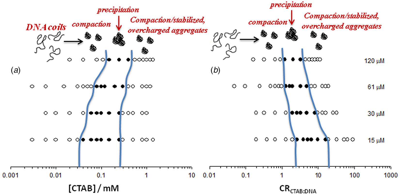
Following the observations for other polymers (see above), because of the inferred hydrophobic character of DNA, binding of surfactants above charge equivalence would be expectable to occur and lead to complexes with a net positive charge and also to re-dissolution, as excess surfactant is added. However, this was not observed in earlier work (Rosa et al., Reference Rosa, Dias, Da Graça Miguel and Lindman2005).
The surfactant−DNA precipitate would also be expected to dissolve with the addition of electrolyte, but by another mechanism, the screening of the electrostatic attraction. Such an effect has been observed for a large number of polyelectrolyte−surfactant systems (Thalberg et al., Reference Thalberg, Lindman and Karlstroem1991). However, long-term observations using a large range of electrolytes and electrolyte concentrations did not indicate any dissolution; the lack of dissolution was referred to as kinetic trapping (not uncommon for large polymers). Carlstedt and Dias (Carlstedt et al., Reference Carlstedt, Lundberg, Dias and Lindman2012) solved this puzzling observation by changing the design of the experiments and making direct observations of the charge of the aggregates by electrophoresis. Strikingly, it was observed that there is a large concentration range, with an excess of surfactant, without any sign of phase separation. Furthermore, it was observed that in this region of excess surfactant, there are aggregates with net positive charge, thus with more surfactant molecules than charges of DNA; the aggregates are negatively charged below charge stoichiometry, as shown from electrophoretic measurements (Fig. 7). This provides direct evidence for the role of hydrophobic interactions in the association and that DNA must be considered as an amphiphilic polymer.
Dynamic light scattering (RH app) and electrophoretic mobility (μe) data for aqueous mixtures of DNA and CTAB, with a constant DNA concentration of 120 μM in nucleotides (40 μg ml−1) and varying CTAB concentration. Adapted from Carlstedt et al. (Reference Carlstedt, Lundberg, Dias and Lindman2012) with permission of ACS.

Other aspects of DNA hydrophobicity
As expected, and as has been documented for some time, many cationic cosolutes, polymers, multivalent metal ions, proteins, and surfactants/lipids, associate with DNA. This is driven by entropic electrostatic interactions and the association is expected to be stronger with increasing charge number and charge density of both cosolutes. For ds-DNA, all these additives typically induce two effects: intermolecular association leading to phase separation and, for dilute solutions, monomolecular compaction. Note that the compaction is a cooperative process which can be viewed as a phase separation on individual DNA molecules.
The association of two DNA strands into the double helix is driven by the hydrophobic interactions between the bases. Polar interactions, associated with the phosphate and carbohydrate groups, counteract the association. Hydrogen bonding and specific packing of the bases control the details of the double-helix structure (Dias and Lindman, Reference Dias, Miguel, Lindman, Dias and Lindman2008).
The electrostatic interactions of DNA have been analysed in detail, as reviewed by different authors in Dias and Lindman (Reference Dias, Miguel, Lindman, Dias and Lindman2008). The hydrophobic interactions have been much less discussed; in particular, the balance between the polar and nonpolar interactions have a deep impact into how DNA interacts with cosolutes, including electrolytes, nonpolar molecules, surfactants, lipids and macromolecules, as well as with interfaces (Dias and Lindman, Reference Dias, Miguel, Lindman, Dias and Lindman2008).
Some additional brief comments on the amphiphilic nature of DNA and its consequences for the solution behaviour are next provided. DNA is clearly different from both block and graft copolymers, but closer to the graft copolymer situation, with hydrophobic grafts on a hydrophilic backbone. However, the segregation between hydrophilic and lipophilic parts is less pronounced in DNA and the force opposing self-assembly stronger, due to a high charge density and a large persistence length. While the detailed structure of the double helix has been extensively investigated, we note that the balance between the hydrophobic force, driving self-assembly, and the opposing force, is very subtle. Two consequences arise: Firstly, the stability of the double helix (ds-DNA) is critically dependent on the electrolyte concentration. In the absence of electrolyte, the opposing force dominates, and the ds-DNA dissociation into ss-DNA may occur (depending on DNA concentration) (Korolev et al., Reference Korolev, Vlasov and Kuznetsov1994). Small amounts of electrolyte, or essentially any cationic cosolute, overcome the electrostatic repulsion and stabilize ds-DNA. Secondly, if the driving force is changed, for example by changing the base composition, there is a significant change in the stability of the double helix.
Manifestations of the hydrophobic interactions include:
-
– Solubilization of hydrophobic molecules (Gaugain et al., Reference Gaugain, Barbet, Capelle, Roques, Le Pecq and Le Bret1978; Howe-Grant and Lippard, Reference Howe-Grant and Lippard1979; Kapuscinski, Reference Kapuscinski1995; Rye and Glazer, Reference Rye and Glazer1995; Spielmann et al., Reference Spielmann, Wemmer and Jacobsen1995; Brabec and Nováková, Reference Brabec and Nováková2006; Irena, Reference Irena2006; Uma Maheswari et al., Reference Uma Maheswari, Rajendiran, Palaniandavar, Thomas and Kulkarni2006; Richards and Rodger, Reference Richards and Rodger2007): This area can be illustrated by the so-called ‘intercalating agents’. Ethidium bromide is a well-known fluorescent dye commonly used to study the interaction between DNA and cosolutes due to its displacement when other molecules bind to DNA. Other dyes binding to DNA are not soluble in water. Recent work has focused on the role of the ligand hydrophobicity on DNA binding and it was found, not surprisingly, that the most hydrophobic compounds have a higher binding affinity to DNA. In this case, however, the ligands did not interact with DNA by intercalation but by hydrophobic interactions with the surface of the DNA, that is, the pockets of the groves. This sort of interaction is common for some fluorescent dyes, such as DAPI and in protein−DNA interactions.
-
– Adsorption on hydrophobic surfaces: It was observed by ellipsometry that, whereas both ds- and ss-DNA molecules adsorb on hydrophobic surfaces, ss-DNA generally adsorbs more preferentially than ds-DNA (Eskilsson et al., Reference Eskilsson, Leal, Lindman, Miguel and Nylander2001; Cárdenas et al., Reference Cárdenas, Braem, Nylander and Lindman2003). Also, while ds-DNA molecules form a very thick and diffuse layer on the surface, the ss-DNA molecules adsorb in a thin layer of ca. 20 Å indicating that the molecules are parallel to the surface (Cárdenas et al., Reference Cárdenas, Braem, Nylander and Lindman2003). This is naturally due to the larger hydrophobicity of the ss-DNA, as each base will serve as an attachment point to the surface overcoming the entropy loss of the adsorption; ss-DNA is much more flexible than ds-DNA. In fact, the bases were shown to have different adsorption properties depending on their hydrophobicity. The purine bases, more hydrophobic due to the two aromatic rings, present larger adsorption than the pyrimidine bases (Sowerby et al., Reference Sowerby, Cohn, Heckl and Holm2001; Chiorcea Paquim et al., Reference Chiorcea Paquim, Oretskaya and Oliveira Brett2006).
-
– Effects of hydrophobic cosolutes on DNA melting: The interactions between DNA and alkyltrimethylammonium bromide salts with short hydrophobic chains and the influence of the chain length on the melting have been previously addressed (Orosz and Wetmur, Reference Orosz and Wetmur1977). It was observed that the melting temperature of DNA decreases linearly with the increase of the hydrophobic group up to the pentyl substitution. Short-chain alcohols showed the same behaviour. The melting temperature of DNA was found to decrease in water/methanol solutions (Geiduschek and Herskovits, Reference Geiduschek and Herskovits1961). Furthermore, the midpoint of the solvent denaturation decreased in the order: methanol, ethanol, propanol; i.e. the secondary structure (interactions between bases) stability was lowered as the length of the aliphatic chain was increased (Geiduschek and Herskovits, Reference Geiduschek and Herskovits1961).
For alkyltrimethylammonium salts there is a striking nonmonotonic variation of the melting point with alkyl chain length, illustrating the balance between interactions. For short alkyl chains the cosolute competes with the association between bases, whereas with longer alkyl chains there is a self-assembly into highly charged aggregates, which interact electrostatically with DNA; with a longer alkyl chain the CAC is lower and the micelles larger.
-
– Differences in interactions of cationic surfactants between ss- and ds-DNA: One other indication that points to the importance of the hydrophobic moieties of DNA on the interaction with cosolutes is the difference in interactions of ss- and ds-DNA with cationic surfactants. It was observed that the precipitation behaviour for DNA – dodecyltrimethylammonium bromide (C12TAB) is different when DNA is in the denaturated or in the double-helix conformation (Rosa et al., Reference Rosa, Dias, Da Graça Miguel and Lindman2005). In this case, the DNA conformation was controlled by the temperature. The fact that C12TAB interacts preferentially with ss-DNA, for low concentrations of surfactant, signifies that the melting temperature of DNA will be shifted to a lower temperature (Rosa et al., Reference Rosa, Dias, Da Graça Miguel and Lindman2005). Other illustrations on the role of hydrophobic interactions in DNA self-assembly (Dias and Lindman, Reference Dias, Miguel, Lindman, Dias and Lindman2008) relate to DNA−protein interactions (Härd and Lundbäck, Reference Härd and Lundbäck1996; Jen-Jacobson et al., Reference Jen-Jacobson, Engler and Jacobson2000; West and Wilson, Reference West and Wilson2002), the dependence of DNA melting on the base sequence and the preparation of DNA chemical and physical gels. Regarding chemical gels (Costa et al., Reference Costa, Miguel and Lindman2007), covalently cross-linked ss- and ds-DNA interact differently with cationic surfactants. On the other hand, it is notable that DNA can form physical gels in combination with hydrophobically modified cationic polymers (Costa et al., Reference Costa, Santos, Antunes, Miguel and Lindman2006). The effects of hydrophobic interactions on DNA condensation has been discussed in several articles (Patel and Anchordoquy, Reference Patel and Anchordoquy2005; Sumi et al., Reference Sumi, Suzuki and Sekino2009; Filippov et al., Reference Filippov, Koňák, Kopečková, Starovoytova, Špírková and Štěpánek2010; Zhou et al., Reference Zhou, Llizo, Wang, Xu and Yang2013; Xiao et al., Reference Xiao, Chen, Wei and Tian2020). Another particularly relevant example of considerable biological significance deserves some attention; DNA, in the eukaryotic cells, exists in the form of the histone−DNA complex chromatin. Although electrostatic interactions between negatively charged DNA and cationic histones make a decisive contribution to chromatin formation and stability, hydrophobic interactions within the histone octamer are critical for the establishment of specific structure of the universal basic unit of chromatin, the nucleosome core particle (NCP) (Fig. 8).
Illustrations of (a) an NCP, (b) the core histones, and (c) the nucleosome array. (a) Two projections of the NCP where DNA is shown as a surface with electrostatic potential (positive in red and negative in blue) and the histone octamer with schematic secondary structure (each of the eight histones is coloured differently). Approximate dimensions of the NCP are indicated. The core histones shown in panel b illustrate the folded domains of each histone shown with the surface coloured according to its electrostatic potential (positive in blue) and hydrophobicity (orange). In panel c, a nucleosome array comprising 12 nucleosomes formed by the wrapping of 147 bp DNA around the histone octamer, is schematically shown. DNA is red and the histone octamer core light grey with histone tails in blue. Reproduced from Berezhnoy et al. (Reference Berezhnoy, Lundberg, Korolev, Lu, Yan, Miguel, Lindman and Nordenskiöld2012) with permission from ACS.

This importance of hydrophobic forces was revealed in experimental studies of systems that included the NCP or model nucleosome arrays (in vitro reconstituted chromatin fibres) in combination with lipids. The addition of lipids resulted in a shift of the delicate balance between hydrophobic and electrostatic forces, dissociation of the NCP and model chromatin, which was accompanied by the transfer of histones from DNA to the lipids and formation of various lamellar lipid−DNA structures (Lundberg et al., Reference Lundberg, Berezhnoy, Lu, Korolev, Su, Alfredsson, Miguel, Lindman and Nordenskiöld2010; Berezhnoy et al., Reference Berezhnoy, Lundberg, Korolev, Lu, Yan, Miguel, Lindman and Nordenskiöld2012, Reference Berezhnoy, Korolev and Nordenskiöld2014).
Another example of how hydrophobic interactions control DNA self-assembly was recently revealed by Wong and co-workers, studying antimicrobial peptides (AMPs) that are amphiphilic ɑ-helices (Lee et al., Reference Lee, Zhang, Di Domizio, Jin, Connell, Hung, Malkoff, Veksler, Gilliet, Ren and Wong2019). This example is of considerable medical importance for understanding activation in immune cells by the proinflammatory activity of AMPs. Comparing the three AMPs melittin, LL37, and buforin and using simulations and synchrotron X-ray diffraction, they showed how the AMP hydrophobicity controlled the peptide's ability to function as subunits that assemble into superhelical protofibrils in the presence of DNA by forming columnar protofibril−DNA nanocrystals (Fig. 9).
Structure of melittin-double-stranded DNA (dsDNA) three-dimensional (3D) tetragonal lattice from molecular simulations verified by X-ray diffraction. View of a melittin-dsDNA square lattice. Columnar dsDNA is coloured red, and the melittin protofibril is coloured green (N to C terminus polarity) and teal (C to N terminus polarity). Reproduced from Lee et al. (Reference Lee, Zhang, Di Domizio, Jin, Connell, Hung, Malkoff, Veksler, Gilliet, Ren and Wong2019) with permission from Nature.

The topic of the role of hydrophobic interactions for the stability of ds-DNA has received much-renewed interest through recent studies by Nordén et al. (Feng et al., Reference Feng, Sosa, Mårtensson, Jiang, Tong, Dorfman, Takahashi, Lincoln, Bustamante, Westerlund and Nordén2019) using a novel perspective. These authors investigated the effect of slightly nonpolar cosolutes on the association between the bases in DNA. They found that additives, such as short-chain PEG, diglyme and dioxane significantly reduced the association. Interestingly, this type of substances reduces the association between surfactant molecules, thus causing demicellization. As an example, the CMC of CTAB was found to increase with increasing PEG concentration, as well as its molar mass (Manna and Panda, Reference Manna and Panda2011).
The addition of water-soluble polymers to DNA solution can lead to DNA compaction by a ‘crowding effect’. Here, there is a large difference between dextran and PEG; as argued by Nordén et al. (Feng et al., Reference Feng, Sosa, Mårtensson, Jiang, Tong, Dorfman, Takahashi, Lincoln, Bustamante, Westerlund and Nordén2019) this fits very well with the amphiphilic properties of DNA since dextran is strongly polar whereas PEG is much less polar. A similar difference in the crowding effect was observed for the compaction of the chromatin (Zinchenko et al., Reference Zinchenko, Chen, Berezhnoy, Wang and Nordenskiöld2020) where PEG results in the complete compaction of T4 DNA reconstituted chromatin fibres into globules while the strongly polar dextran causes only slight chromatin compaction. The compaction of T4 DNA alone occurs in the presence of PEG (Zinchenko et al., Reference Zinchenko, Berezhnoy, Chen and Nordenskiöld2018) but not in concentrated solutions of dextran (Zinchenko et al., Reference Zinchenko, Chen, Berezhnoy, Wang and Nordenskiöld2020).
Important contributions regarding the balance between hydrogen-bonding and hydrophobic interactions are due to Frank-Kamenetskii and co-workers (Protozanova et al., Reference Protozanova, Yakovchuk and Frank-Kamenetskii2004; Yakovchuk et al., Reference Yakovchuk, Protozanova and Frank-Kamenetskii2006; Vologodskii and Frank-Kamenetskii, Reference VologodskII and Frank-Kamenetskii2018). The most recent one is also the most comprehensive, including an extensive analysis of the large body of earlier works. A major point is that they found stacking enthalpy in the range of −8.2 to −10.2 kcal mol−1 (depending on the bp type). However, they obtained estimates for the base pairing of ΔHbpA⋅T = 0.9 ± 1 kcal mol−1 (for the AT bp) and ΔHbpG⋅C = 0.6 ± 1 kcal mol−1 (for the GC bp), concluding that the contribution to double-helix formation from base pairing has an enthalpy value that is insignificant compared to the stacking enthalpy.
Charging up cellulose counteracts hydrophobic association and facilitates dissolution
From a theoretical perspective, the dissolution of cellulose in aqueous media has been shown to be energetically unfavourable because the entropy loss due to water–cellulose interactions is not balanced by the related entropy gain from the increased chain conformations upon dissolution (Bergenstråhle et al., Reference Bergenstråhle, Wohlert, Himmel and Brady2010; Parthasarathi et al., Reference Parthasarathi, Bellesia, Chundawat, Dale, Langan and Gnanakaran2011; Bao et al., Reference Bao, Qian, Lu and Cui2015).
This is verified in practice since cellulose is not soluble in water; thus, the cellulose behaviour in solution is mostly analysed in solvent systems of a rather complex composition (i.e. concentrated salt solutions, ionic liquids, organic/salt mixtures, etc.) (Medronho and Lindman, Reference Medronho and Lindman2014, Reference Medronho and Lindman2015). As mentioned, cellulose solubility in aqueous solutions is typically observed at extreme pHs and literature has largely been attributing this phenomenon on breaking hydrogen bonds. Instead, it has been argued that such enhanced solubility at extreme pH values is a clear manifestation of a polyelectrolyte-like behaviour where cellulose molecules attain net charge due to protonation/deprotonation.
If the polymer is ionized (for instance, by adding base), the energy balance changes since the counterions and Coulombic interactions contribute largely to the entropy gain (Schneider and Linse, Reference Schneider and Linse2002, Reference Schneider and Linse2003). Consequently, polymers that are charged are generally soluble in water, even if they are not markedly polar (Lindman et al., Reference Lindman, Medronho, Alves, Costa, Edlund and Norgren2017). The polyelectrolyte nature of cellulose has been subjected of numerous investigations in the past, mainly regarding the controversy as to whether the reaction with alkali yields a true alcoholate or an addition compound without ionization of the cellulose (Pennings and Prins, Reference Pennings and Prins1962). It was found that the osmotic pressure data could be well described considering cellulose as a weak polyacid. The ionization of the hydroxyls of glucose are well known and easily admitted to other related biomacromolecules, such as amylose (Bertoft, Reference Bertoft2017). Citing Bertoft, ‘…at pH > 13 the hydroxyl groups on the glucose residues become negatively charged and the molecule expands to its largest volume.’ Surprisingly, this behaviour has been underrated for cellulose.
One possible explanation relies on the fact that, classically, cellulose solubility/swelling studies have been performed by plotting data as a function of the NaOH concentration (in %), and not as a function of pH as typically done in other systems, such as proteins. This may have contributed to not giving adequate relevance to the effect of pH on ionization.
The finding of maxima for the solubility/swelling of cellulose on increasing the NaOH concentration could be interpreted as a maximum produced by a Donnan effect (e.g. as made by Neale (Kasbekar and Neale, Reference Kasbekar and Neale1947)), similar to that already seen in other charged polymers, such as collagen when going into extreme pHs (Bowes and Kenten, Reference Bowes and Kenten1948).
In the late 1990s, cellulose ionization was inferred from NMR data by considering that not all OH groups are required to be fully ionized, but form transient dissociated structures of relatively short duration (Isogai, Reference Isogai1997).
This hypothesis found support in recent electrophoretic NMR studies where it was shown that cellobiose can act as a weak acid undergoing two base-independent (KOH and NaOH) dissociation states at pHs of 12 and 13.5 (Bialik et al., Reference Bialik, Stenqvist, Fang, Östlund, Furó, Lindman, Lund and Bernin2016) (Fig. 10).
Left: Effective charge of cellobiose as a function of the pH of the solution either using KOH (filled circles) or NaOH (empty circles). Right: Cellulose configurations in the last frame of a 1 μs simulation for (a) neutral and (b) deprotonated cellodecaose. Taken from Bialik et al. (Reference Bialik, Stenqvist, Fang, Östlund, Furó, Lindman, Lund and Bernin2016) with permission of ACS.

Additional MD results further confirmed this ionization effect showing that charging up cellulose prevents its aggregation.
We also note that cellulose dissolution in systems based on aqueous metal complexes (Burchard et al., Reference Burchard, Habermann, Klüfers, Seger and Wilhelm1994; Klüfers and Schuhmacher, Reference Klüfers and Schuhmacher1994; Saalwächter et al., Reference Saalwächter, Burchard, Klüfers, Kettenbach, Mayer, Klemm and Dugarmaa2000) or zinc chloride (Letters, Reference Letters1932; Xu and Chen, Reference Xu and Chen1999) requires ionization of OH-groups. This provided further evidence to the deprotonation of cellulose in basic media. In some cases, cellulose decreases its solubility in basic solution upon addition of ionic or non-ionic additives and this can be understood from the overall decrease in entropy of the system (Medronho et al., Reference Medronho, Duarte, Alves, Antunes, Romano and Valente2016; Alves et al., Reference Alves, Medronho, Antunes, Topgaard and Lindman2016a, Reference Alves, Medronho, Antunes, Topgaard and Lindman2016b).
Cellulose amphiphilicity
It is striking that, through the years, cellulose insolubility in water has been attributed to strong cellulose–cellulose hydrogen bonds. This view has been rooted in the cellulose community for decades, but clearly conflicts with our fundamental understanding of water as a solvent. It is important to realize that during the dissolution process, intermolecular interactions in the solute have to be broken, such as the hydrogen bonds between cellulose molecules, which are unfavourable for dissolution. However, new interactions between the solute and the solvent molecules are established and it is the final balance of all different interactions that govern the outcome of the dissolution process. When considering cellulose in water, not only hydrogen bonding among cellulose−cellulose is important but also between cellulose and water and among water molecules. It appears that these different hydrogen bonds are not markedly different in magnitude and thus aqueous insolubility cannot be attributed to hydrogen bonding. The energy needed to break hydrogen bonding represents a fraction of the total free energy required to dissolve cellulose. This has been validated in a detailed analysis of the balance of interactions by Bergenstråhle et al. and in other related reports (Bergenstråhle et al., Reference Bergenstråhle, Wohlert, Himmel and Brady2010; Parthasarathi et al., Reference Parthasarathi, Bellesia, Chundawat, Dale, Langan and Gnanakaran2011; Bao et al., Reference Bao, Qian, Lu and Cui2015).
An analogous conclusion can be reached if we compare a similar number of glucose units, but distributed in different block lengths (Fig. 11).
Schematic representation of glucose-based oligomers with different degrees of polymerization.

Although the number of established hydrogen bonds is pretty much the same, shorter chains remain in solution while the longer ones do aggregate. Since insolubility cannot be attributed to hydrogen bonding other causes must be identified. As earlier discussed for DNA, the cause of insolubility of the longer-chain polymers is related to entropy; the longer polymer chains self-aggregate and release their bound solvent molecules thus maximizing the entropy of the system. On the other hand, the shorter chains still have a fair degree of movement and random positions, contributing to the total entropy of the system, and can remain in solution.
For the last decade, it has been argued that cellulose is strikingly amphiphilic and that its aqueous insolubility should have a significant contribution from hydrophobic interactions (Lindman et al., Reference Lindman, Karlström and Stigsson2010; Medronho et al., Reference Medronho, Romano, Miguel, Stigsson and Lindman2012). For instance, returning to the dissolution process at high pH, we have observed that cellulose dissolution becomes more favourable if the disruption of hydrophobic interactions accompanies the ionization. This can be done by using organic hydroxides, such as tetrabutylammonium hydroxide (TBAH), which are more efficient than their inorganic counterparts (NaOH) because the cations of the former are capable of weakening the hydrophobic interactions while the inorganic cations are not (Alves et al., Reference Alves, Medronho, Antunes, Romano, Miguel and Lindman2015; Gubitosi et al., Reference Gubitosi, Duarte, Gentile, Olsson and Medronho2016).
Unsurprisingly, these claims on the role of hydrophobic interactions on cellulose solubility are far from being original and similar conclusions have been drawn in much earlier publications (French et al., Reference French, Miller and Aabloo1993, Reference French, Dowd, Cousins, Brown, Miller, Saddler and Penner1996; Cousins and Brown, Reference Cousins and Brown1995; Nishiyama et al., Reference Nishiyama, Langan and Chanzy2002). However, such contributions have been mostly neglected and instead there has been a massive flood of publications claiming hydrogen bonding as the principal cause of cellulose insolubility in water. The complex interplay between H-bonding, ionization effects, and hydrophobic interactions is crucial to control dissolution, regeneration, gelation, and related phenomena (Lindman et al., Reference Lindman, Medronho, Alves, Costa, Edlund and Norgren2017).
Segregation between polar and nonpolar groups in cellulose
Several observations stand out regarding the fundamental importance of cellulose amphiphilicity and concomitant role of hydrophobic interactions in the behaviour of cellulose in aqueous systems (Medronho et al., Reference Medronho, Duarte, Alves, Antunes, Romano and Lindman2015). Looking at the cellulose molecular structure, cellulose chains consist of D-pyranose rings connected by β-1,4 glycosidic bonds where the polar hydroxyl groups render cellulose hydrophilic, while the nonpolar backbones of carbon rings make it hydrophobic (Biermann et al., Reference Biermann, Hädicke, Koltzenburg and Müller-Plathe2001; Yamane et al., Reference Yamane, Aoyagi, Ago, Sato, Okajima and Takahashi2006; Diddens et al., Reference Diddens, Murphy, Krisch and Müller2008; Miyamoto et al., Reference Miyamoto, Umemura, Aoyagi, Yamane, Ueda and Takahashi2009; Youssefian and Rahbar, Reference Youssefian and Rahbar2015).
The distinction between the hydrophilic lateral rim and the hydrophobic top and bottom of a cellulose molecule renders cellulose clear amphiphilicity. This has been very early recognized, for example in the work of Hermans (Reference Hermans1949) (Fig. 12).
The nuclear frame of a cellobiose residue. The centres of gravity of the atoms of the ring are distributed over two parallel planes. The hydrophobic H atoms are above and below these planes and laterally there are the hydrophilic OH groups. Taken from Hermans (Reference Hermans1949) with the permission of John Wiley and Sons, Inc.

Quoting Hermans: ‘…the atoms of the (cellulose) ring can be distributed over two parallel planes, above and below these plans are the hydrogen atoms and laterally we have the hydroxyl groups. The cellulose chain exhibits two hydrophobic and two hydrophilic boundary surfaces.’
Due to the hydrophobic properties of the glucopyranose plane, the cellulose chains can stack via hydrophobic interactions and can form a sheet-like structure that should be disrupted for dissolution to occur. This was already documented by Sponsler's diffraction work (Sponsler, Reference Sponsler1931) and later by Warwicker and Wright (Warwicker and Wright, Reference Warwicker and Wright1967).
Additives may weaken the hydrophobic interactions in cellulose
The addition of specific additives, such as urea, thiourea, guanidine and their derivatives weakens hydrophobic interactions thus facilitating cellulose dissolution (Lilienfeld, Reference Lilienfeld1924, Reference Lilienfeld1927; Zhou and Zhang, Reference Zhou and Zhang2000; Cai and Zhang, Reference Cai and Zhang2005; Cai et al., Reference Cai, Liu and Zhang2006, Reference Cai, Zhang, Chang, Cheng, Chen and Chu2007, Reference Cai, Zhang, Liu, Liu, Xu, Chen, Chu, Guo, Xu, Cheng, Han and Kuga2008; Egal et al., Reference Egal, Budtova and Navard2008; Qi et al., Reference Qi, Chang and Zhang2008; Ruan et al., Reference Ruan, Lue and Zhang2008; Liu and Zhang, Reference Liu and Zhang2009). In aqueous solutions, these additives cause, inter alia, protein denaturation and demicellization of surfactant aggregates (Tanford, Reference Tanford1964; Piercy et al., Reference Piercy, Jones and Ibbotson1971; Briganti et al., Reference Briganti, Puvvada and Blankschtein1991; Zangi et al., Reference Zangi, Zhou and Berne2009). In the case of cellulose dissolution, it was recently shown by a set of unusual techniques (cryo-transmission electronic microscopy, diffusion wave spectroscopy and solid-state nuclear magnetic resonance) that cellulose solubility in aqueous alkali is significantly improved by urea, as seen in Fig. 13 (Alves et al., Reference Alves, Medronho, Filipe, E. Antunes, Lindman, Topgaard, Davidovich and Talmon2018).
Cryo-transmission electronic microscopy (cryo-TEM) images of 0.5 wt % MCC dissolved in (a) 8 wt % NaOH(aq.) solution and (b) in 8 wt % NaOH(aq.)/12 wt % urea system. Scale bars correspond to 100 nm.

Besides, this additive remarkably affects the solution stability, preventing thermal gelation in certain conditions (Swensson et al., Reference Swensson, Larsson and Hasani2020a). Interestingly, urea has been shown to concentrate on cellulose surfaces in solutions of aqueous urea (Bergenstråhle-Wohlert et al., Reference Bergenstråhle-Wohlert, Berglund, Brady, Larsson, Westlund and Wohlert2012; Chen et al., Reference Chen, Nishiyama, Wohlert, Lu, Mazeau and Ismail2017; Walters et al., Reference Walters, Mando, Matthew Reichert, West, West and Rabideau2020).
This is also in agreement with the recent work of Swensson et al. where the authors show that adding urea to solutions of NaOH and/or tetramethylammonium hydroxide (TMAH) improves dissolution and can successfully be used together with these bases (Swensson et al., Reference Swensson, Larsson and Hasani2020b). Interestingly, adding urea to benzyltrimethylammonium hydroxide (known as Triton B) solutions did not seem to have a significant effect on cellulose dissolution, and the solvatochromic probes indicated that urea might be excluded from interacting with cellulose in the presence of Triton B. Both urea and Triton B are believed to weaken the hydrophobic effect by replacing water around the pyranose ring but, most likely, this effect is more pronounced for Triton B than for urea (Swensson et al., Reference Swensson, Larsson and Hasani2020b). In a related work, Wei et al. argue that the role of urea in tetrabutylammonium hydroxide (TBAH)/urea aqueous solvents can be regarded as a hydrophobic contributor, where the amphiphilic properties of the solvent system can be tuned. The authors suggest that for a suitable amphiphilicity similar to that of the crystal surface of pristine cellulose, the interfacial resistance between the solvent and the crystal surface can be reduced so that the crystalline areas of cellulose can be effectively infiltrated and subsequently dissolved by the solvent (Wei et al., Reference Wei, Meng, Cui, Jiang and Zhou2017). This same conclusion was also reached regarding the role of urea in enhancing the solubility in aqueous solutions of amino acids and proteins (Whitney and Tanford, Reference Whitney and Tanford1962; Nozaki and Tanford, Reference Nozaki and Tanford1963; Zangi et al., Reference Zangi, Zhou and Berne2009), and also of chitin chains (which are structurally very similar to cellulose) (Huang et al., Reference Huang, Zhong, Zhang and Cai2020). In this latter case, the presence of urea changes the chemical shifts very little in the α-chitin/KOH/water system, confirming that urea solubilized chitin chains by preferentially solvating the hydrophobic parts of the chitin backbone without interfering with the chitin chain conformation in the aqueous KOH/solution.
Similarly to urea, the addition of a zwitterionic surfactant to cellulose dissolved in an alkali-based solvent can prevent the gelation of the dope. After dissolution, as temperature increases, gelation of the cellulose dope is observed; the gelation temperature, T g, can be estimated from the crossover of the storage (G′) and loss (G′′) moduli. The addition of the zwitterionic surfactant to the cold alkali solvent system led to a shift in gelation temperature of ca. 10°C (Fig. 14). The same behaviour was observed using a concentrated zinc chloride aqueous solution (Medronho et al., Reference Medronho, Duarte, Alves, Antunes, Romano and Lindman2015).
Elastic modulus, G′ (filled symbols), and viscous modulus, G′′ (open symbols) as a function of temperature for 3.5 wt% microcrystalline cellulose samples dissolved in a 10 wt% NaOH/H2O solvent system: (a), without cocamidopropylbetaine and (b) with cocamidopropylbetaine. Constant heating rate of 1°C min−1 at 0.5 Hz. The temperature of gelation (G′ = G′′) is increased by ca. 10°C in the presence of the amphiphilic additive. The vertical dashed grey line indicates the transition region. Taken from Medronho et al. (Reference Medronho, Duarte, Alves, Antunes, Romano and Lindman2015) with the permission of De Gruyter.

MD simulation studies of the interaction of cellulose with different compounds in aqueous media have confirmed that, in cellulose crystals, apart from hydrogen bonding, hydrophobic interactions also play a substantial role (Alqus et al., Reference Alqus, Eichhorn and Bryce2015; Chen et al., Reference Chen, Nishiyama, Wohlert, Lu, Mazeau and Ismail2017). The same was concluded regarding the absorption of a soluble hEGF protein to the cellulose surface. Interestingly, it was found that the hEGF protein binds to both the (010) and (100) cellulose surfaces through different regions of the protein which contain both polar and apolar residues. In the case of the (010) surface, the amino acids involved in adsorption are mostly polar whereas in the case of adsorption at the (100) surface the amino acids involved are preferentially apolar. This result suggests that the simultaneous hydrophilic and hydrophobic character of cellulose induces a substantial interaction of cellulose with proteins (which are also amphiphilic) (Malaspina and Faraudo, Reference Malaspina and Faraudo2019).
Organic and inorganic counterions interact differently with cellulose
Solutions of organic acids or bases are superior solvents to those of inorganic ones. For instance, cellulose dissolution in TBAH is observed to proceed down to the molecular level (Gubitosi et al., Reference Gubitosi, Duarte, Gentile, Olsson and Medronho2016), while NaOH does not dissolve cellulose molecularly (Alves et al., Reference Alves, Medronho, Antunes, Romano, Miguel and Lindman2015); it rather leaves aggregates of high crystallinity stable in the cellulose dope (Pereira et al., Reference Pereira, Duarte, Nosrati, Gubitosi, Gentile, Romano, Medronho and Olsson2018) (Fig. 15).
Scanning electron microscopy images of the cellulose solutions after being deposited onto a glass lamella followed by solvent evaporation. Left: cellulose dissolved in 2 M NaOH aqueous solvent; right: cellulose dissolved in the 1.5 M TBAH aqueous solvent. The scale bar represents 5 μm. Adapted from Alves et al. (Reference Alves, Medronho, Antunes, Romano, Miguel and Lindman2015) with the permission of Elsevier.

It was inferred that 1.2 TBA+ ions bind per anhydroglucose unit and this was later supported by detailed scattering studies where the SAXS data suggest the presence of a solvation shell enriched in TBA+ ions around the cellulose molecules. The TBA+ cation is suggested to interact by electrostatic interactions with the (partially) deprotonated hydroxyl groups of cellulose, in addition to hydrophobic interactions due to its amphiphilicity (Gentile and Olsson, Reference Gentile and Olsson2016). Furthermore, cellulose solubility has been observed to increase as a function of increasing cation hydrophobicity (Wang et al., Reference Wang, Liu, Chen, Zhang and Lu2018). In a series of aqueous solutions of tetraalkyl ammonium hydroxides, namely tetramethyl ammonium hydroxide, triethylmethyl ammonium hydroxide, tetraethyl ammonium hydroxide, benzyltrimethyl ammonium hydroxide, benzyltriethyl ammonium hydroxide, and two inorganic salts, NaOH and LiOH, the authors reported a marked improvement on the dissolution capacity with the use of more hydrophobic cations, as well as increased stability against chain aggregation and gelation (Fig. 16). On the other hand, the solubility of cellulose followed the Hofmeister series, and cations with greater kosmotropicity originating from their larger hydrophobicity exhibited higher dissolution power (Wang et al., Reference Wang, Liu, Chen, Zhang and Lu2018). As discussed by Moelbert et al. kosmotropic cosolvents added to an aqueous solution are known to promote the aggregation of hydrophobic solute particles (Moelbert et al., Reference Moelbert, Normand and De Los Rios2004). The dominant effect of a kosmotropic substance is to enhance the water structuring. The consequent preferential exclusion both of cosolvent molecules, from the solvation shell of hydrophobic particles, and of these particles from the solution, leads to a stabilization of the aggregates. The origin of the kosmotropic (and chaotropic) effects appears to lie primarily in their influence on the solvent, rather than in direct interactions between cosolvent and solute. The microscopic origin of these preferential effects lies in the energetically favourable enhancement of hydrogen-bonded water structure in the presence of a kosmotropic cosolvent. In a more macroscopic interpretation, the preferential hydration of solute particles by kosmotropic agents can be considered to strengthen the solvent-induced, effective hydrophobic interaction between solute particles, thus stabilizing their aggregates (Kita et al., Reference Kita, Arakawa, Lin and Timasheff1994; Timasheff and Arakawa, Reference Timasheff, Arakawa and Creighton1997; Franks, Reference Franks2002).
Solubility of cellulose in aqueous quaternary ammonium hydroxides as a function of the cation hydrophobicity. Adapted from Wang et al. (Reference Wang, Liu, Chen, Zhang and Lu2018) with permission of the Royal Society of Chemistry.

Cellulose regeneration is also controlled by hydrophobic interactions
Cellulose regeneration studies are as significant as dissolution studies and the role of cellulose amphiphilicity has been demonstrated in different reports. For instance, it has been suggested that the polarity of the coagulant governs the hydrophobic interactions between the polymer chains during regeneration (Östlund et al., Reference Östlund, Idström, Olsson, Larsson and Nordstierna2013). This hypothesis is in accordance with the discussion on cellulose amphiphilicity, which would indicate preferential interactions depending on the polarity of the coagulant. Among other interesting results, it was recently found that the water contact angle of regenerated cellulose films increases with lower water solubility of the coagulant. Most likely, this is due to cellulose amphiphilicity where the exposition of the hydrophobic areas to a polar environment is energetically unfavourable, thus leading to the reorientation of the more hydrophilic parts of cellulose (OH groups) towards the film interface (From et al., Reference From, Larsson, Andreasson, Medronho, Svanedal, Edlund and Norgren2020).
Another striking evidence for the critical role of hydrophobic interactions in regeneration was provided by (Isobe et al., Reference Isobe, Kimura, Wada and Kuga2012), who followed the coagulation of cellulose solutions prepared in the aqueous alkali-urea solvent by time-resolved synchrotron X-ray scattering. The authors have shown that when the medium surrounding the cellulose molecules becomes energetically unfavourable for molecular dispersion, regeneration is triggered. The initial process is suggested to occur via stacking of the hydrophobic glucopyranoside rings, driven by hydrophobic interactions, followed by their mutual association via hydrogen bonding to form a hydrated form of cellulose II (Isobe et al., Reference Isobe, Kimura, Wada and Kuga2012) (Fig. 17).
Synchrotron X-ray diffraction profiles of cellulose solution under regeneration by 5 wt% aq. Na2SO4, control: 10 wt% cellulose solution without coagulant; (a) measured at 2 mm away from the boundary with coagulant and 180 min after coagulant introduction; (b) 2.5 mm, 195 min; (c) 1.75 mm, 190 min; (d) 1.5 mm, 185 min; (e) 1.5 mm, 200 min; (f) 1.5 mm, 270 min, and complete regeneration: 1.5 mm, 1 week. q denotes the scattering vector (2π/d). Adapted from Isobe et al. (Reference Isobe, Kimura, Wada and Kuga2012) with permission of Elsevier.

These findings are essential in attempts to control cellulose regeneration in dependence of the desired product properties. MD simulations have supported this picture when analysing the formation of regenerated cellulose from aqueous cellulose solutions (Miyamoto et al., Reference Miyamoto, Umemura, Aoyagi, Yamane, Ueda and Takahashi2009).
In the same direction, it was recently shown that the gelation phenomenon of cellulose solutions prepared in cold alkali occurs due to a crystallization and/or precipitation process where an effective cross-linked network would be established with different cellulose chains participating in more than one crystallite and thus acting as bridging points (Pereira et al., Reference Pereira, Duarte, Nosrati, Gubitosi, Gentile, Romano, Medronho and Olsson2018). It was observed that the progressively increased number of hydrophobic junction zones between cellulose chains (and cellulose crystallites) promoted by a temperature increase can be mitigated using appropriate additives, such as surfactants and urea, which are capable of reducing the hydrophobic interactions responsible for cellulose aggregation. Another striking observation, somehow related to cellulose regeneration, is that the biosynthesis of cellulose has been shown to be substantially influenced by the presence of hydrophobic compounds (Haigler et al., Reference Haigler, Brown and Benziman1980, Reference Haigler, White, Brown and Cooper1982; Glasser et al., Reference Glasser, Atalla, Blackwell, Malcolm Brown, Burchard, French, Klemm and Nishiyama2012)
Ionic liquids are good solvents for cellulose
Cellulose is insoluble in water as well as in hydrocarbons but is soluble in a number of solvents displaying a wide range of characteristics. As discussed above, cellulose shows distinct polar and nonpolar regions, thus is amphiphilic. Therefore, a compatibility with solvents, which are also amphiphilic can be expected and this is indeed found. In particular have ionic liquids (ILs) received interest and a large number of them have been found to be excellent solvents of cellulose. Whereas our focus in this review is on aqueous systems, ILs offer an interesting comparison regarding driving forces.
A typical IL is constituted by an organic cation and a strongly polar anion. They are strongly cohesive solvents as shown by the self-assembly of surfactants with several characteristics similar to those of aqueous solutions (Anderson et al., Reference Anderson, Pino, Hagberg, Sheares and Armstrong2003; Fletcher and Pandey, Reference Fletcher and Pandey2004; Patrascu et al., Reference Patrascu, Gauffre, Nallet, Bordes, Oberdisse, De Lauth-Viguerie and Mingotaud2006; Araos and Warr, Reference Araos and Warr2008; Greaves and Drummond, Reference Greaves and Drummond2008; Inoue and Yamakawa, Reference Inoue and Yamakawa2011; Misono et al., Reference Misono, Sakai, Sakai, Abe and Inoue2011). So, for example, non-ionic surfactants micellize with CMCs that strongly decrease with increasing alkyl chain length. The CMCs are much higher than in water, thus the ‘solvophobicity’ is much weaker. (Because of the electrostatic interactions it is more difficult to make a comparison for ionic surfactants.)
The balance between interactions between cellulose and ILs is expected to be quite different than between cellulose and water. In particular since nonpolar groups are present we can expect hydrogen bonding to play an important role. Recently, El Seoud et al. using multi-parameter solvent descriptor correlations, have quantified the relative importance of cellulose−solvent interactions. Their findings in an extensive series of different ionic liquids, strongly suggest that an efficient cellulose solvent should disrupt both the inter- and intramolecular hydrogen bonding in cellulose and the solvophobic interactions arising from the marked amphiphilic character of the biopolymer (El Seoud et al., Reference El Seoud, Bioni and Dignani2021).
As discovered some time ago, ILs are among the most efficient dissolution systems for cellulose (Swatloski et al., Reference Swatloski, Spear, Holbrey and Rogers2002; Zhu et al., Reference Zhu, Wu, Chen, Yu, Wang, Jin, Ding and Wu2006). Their superior dissolution performance has been ascribed to their ability to disrupt the extensive H-bond network and solvophobic interactions present in cellulose. From a structural point of view, ILs are strongly amphiphilic and can be regarded as weak surfactants. As an example, in Fig. 18, the molecular structure of 1-ethyl-3-methylimidazolium acetate, [EMIM][Ac], is shown emphasizing the asymmetry in ion size and charge distribution. This is a powerful ionic liquid solvent for cellulose (and lignocellulose biomass) dissolution (Sun et al., Reference Sun, Rahman, Qin, Maxim, Rodríguez and Rogers2009).
Structure of 1-ethyl-3-methylimidazolium acetate.

Therefore, ILs fit well into the picture of solvophobic interactions in cellulose dissolution. This has been experimentally validated, for instance, in the work of Xu et al. where the cation structure was systematically modified while the anion was kept constant. In the binary solvent mixture Cx MeIm AcOs/dimethyl sulphoxide (DMSO), where x, Me, Im, AcO refer to the number of carbon atoms in the IL side chain, methyl, imidazolium and acetate, respectively, it was found that the dissolution efficiency increases from C2 MeIm AcO to C4 MeIm AcO and then decreases for C8 MeIm AcO (Xu et al., Reference Xu, Cao, Wang and Ma2015). A related work by Kostag et al. reported similar results for quaternary ammonium ILs (Kostag and El Seoud, Reference Kostag and El Seoud2019). The negative enthalpy was taken as support for the formation of hydrogen bonds between acetate and OH-groups and cation-cellulose solvophobic interactions (Kostag et al., Reference Kostag, Pires and El Seoud2020). Theoretical work has been growing fast in this area and data support the critical role of solvophobic interactions. For instance, Mostofian et al. conducted all-atom MD simulations of a 36-chain cellulose microfibril in the ionic liquid [Bmim][Cl] and water for 100 ns. The authors found that [Cl]– interacted preferentially with hydroxyl groups in different cellulose layers while the [Bmim]+ stacked on the nonpolar cellulose surface, stabilizing the detached cellulose chains (Li et al., Reference Li, Wang, Liu and Zhang2018). Similar conclusions have been reached by Ishida using [C2MIm][OAc] as the solvent system (Ishida, Reference Ishida2020). Other related MD studies have generally concluded that the nonpolar cations interact via van der Waals forces with the nonpolar backbone of cellulose while the anion, which is typically polar, forms strong hydrogen bonds with cellulose's hydroxyl groups (Liu et al., Reference Liu, Sale, Holmes, Simmons and Singh2010; Gross et al., Reference Gross, Bell and Chu2011; Rabideau et al., Reference Rabideau, Agarwal and Ismail2014; Xiong et al., Reference Xiong, Zhao, Hu, Zhang and Cheng2014; Wang et al., Reference Wang, Lyu, Sun, Lu, Liu, Zhuang and Zhang2017; Walters et al., Reference Walters, Mando, Matthew Reichert, West, West and Rabideau2020). Neither anions nor cations alone cover all of the strongly attractive interactions within glucose residues; their coupled actions are necessary. Overall, the charge density (hardness and volume of the anion), and the volume, rigidity, Lewis acidity, and nonpolar character of the cation are now regarded as determinant for cellulose dissolution (Kostag et al., Reference Kostag, Gericke, Heinze and El Seoud2019; El Seoud et al., Reference El Seoud, Kostag, Jedvert and Malek2020).
The amphiphilicity of ILs finds parallelism in other good solvents for cellulose, such as N-methylmorpholine N-oxide (Perepelkin, Reference Perepelkin2007) or the above-mentioned aqueous alkylammonium hydroxides (Abe et al., Reference Abe, Kuroda and Ohno2015).
Other manifestations of cellulose amphiphilicity: emulsion stabilization
It is generally assumed that natural starch and cellulose cannot stabilize emulsions. However, since cellulose behaves as an amphiphilic polymer, its adsorption onto the oil−water interfaces is indeed expected to occur. Recent studies have found that cellulose nanocrystals display amphiphilic properties and can be used in the formation of stable emulsions (Paximada et al., Reference Paximada, Tsouko, Kopsahelis, Koutinas and Mandala2016; Vasconcelos et al., Reference Vasconcelos, Feitosa, Da Gama, Morais, Andrade, De Souza Filho and Rosa2017). In the work of (Kalashnikova et al., Reference Kalashnikova, Bizot, Cathala and Capron2012) it was further suggested that crystals with low surface charge favour the stability of emulsions suggesting that the amphiphilic nature of cellulose is the main driving force for the stabilization. Although less common, emulsion formation has been observed not only using cellulose crystals (stabilized by a Pickering-like mechanism) but also using molecularly dissolved cellulose where the interfacial tension between oil and the aqueous medium is found to be lowered by the molecularly dissolved cellulose (Costa et al., Reference Costa, Mira, Benjamins, Lindman, Edlund and Norgren2019). This decrease in the interfacial tension is similar in magnitude to that displayed by non-ionic cellulose derivatives.
Molecularly dissolved cellulose is expected to behave close to typical cellulose derivatives, but it has been much less explored due to the well-known cellulose dissolution limitations. Recent molecular dynamics simulations have shown that molecularly dispersed cellulose gradually assembles, eventually surrounding the oil droplet and stabilizing the formed emulsion (Miyamoto et al., Reference Miyamoto, Rein, Ueda, Yamane and Cohen2017). This has been recently observed in practice by cryo-SEM (Costa et al., Reference Costa, Rosa, Filipe, Medronho, Romano, Liberman, Talmon and Norgren2021), (Fig. 19).
Representative cryo-SEM images [(a) secondary and (b) backscattered electron images] of the emulsions prepared with 1.0 wt.% cellulose previously dissolved in 8 wt.% NaOH/6 wt.% thiourea. In (b) the darker areas correspond to the oil domains (white arrows), while the water domains are lighter. The brightest areas correspond to cellulose (arrowheads). The black arrowhead in (a) points to the cellulose layer surrounding the oil that had been plucked away by the fracturing of the cryo-specimen. Taken from Costa et al. (Reference Costa, Rosa, Filipe, Medronho, Romano, Liberman, Talmon and Norgren2021) with permission of Elsevier.

The interfacial activity of cellulose indicates a significant amphiphilic character and that the interfacial activity of cellulose derivatives is not only related to the derivatization but inherent in the cellulose backbone. This finding suggests that cellulose would have the ability to stabilize dispersions, like oil-in-water emulsions in a similar way as a large number of cellulose derivatives, such as methylcellulose, hydroxyethylcellulose, hydroxypropyl methylcellulose and ethyl hydroxyethyl cellulose (Sheth et al., Reference Sheth, Mcvean and Mattocks1962; Yonekura et al., Reference Yonekura, Hayakawa, Kawaguchi and Kato1998; Schulz and Daniels, Reference Schulz and Daniels2000; Melzer et al., Reference Melzer, Kreuter and Daniels2003; Costa et al., Reference Costa, Mira, Benjamins, Lindman, Edlund and Norgren2019).
Conclusions
Amphiphilic molecules have a large tendency to self-assemble in water. For simple amphiphiles with well-separated polar and nonpolar parts, like in surfactants and block copolymers, simple well-defined structures with extensive nonpolar regions intermixed with water regions are formed. DNA and cellulose also self-assemble in water but because of the distribution of nonpolar groups, special structures form. For DNA, the double helix is the most common structure. For cellulose, it is more unclear and it appears that the state of cellulose in a homogeneous solution can be different for different solvents; in many cases, cellulose molecules are aggregated and even show signs of crystallinity, in others non-aggregated molecules appear.
DNA, cellulose and surfactants are very different, but it is striking that the balance between hydrophilic and hydrophobic interactions has common features; a comparison between the different systems appears fruitful for our understanding. In much of the literature, the driving force for the association of DNA and cellulose has been ascribed to hydrogen bonding. Regarding the formation of the DNA double helix, we argue that hydrogen bonding has been overemphasized and that the driving force is instead due to base stacking; in the nonpolar environment formed due to hydrophobic interactions, hydrogen bonds form (and provide the specificity) but they do no drive association. The insolubility of cellulose in water has been ascribed, in most literature, to strong hydrogen bonds between cellulose molecules. Again, we stress that the association of cellulose molecules in an aqueous environment is driven by hydrophobic interactions; analogously with DNA, the nonpolar domains formed allow for hydrogen bonding between cellulose molecules.
These arguments get strong support from theoretical work but also in studies where the hydrophobic interactions have been weakened by additives. Thus, the same additives that reduce the stability of surfactant aggregates also weaken the stability of the double helix of DNA and increase the aqueous solubility of cellulose. To date a very limited number of additives have been studied in relation to base-stacking in DNA and cellulose dissolution and regeneration; it appears clear that further work on modifying the hydrophobic interaction is fruitful and that simple surfactant systems can offer an excellent basis for such work. It is believed that the same considerations as discussed in this review apply to many other biomacromolecules, including other polysaccharides. For water-soluble proteins, it has been recognized, for a long time, that there is a relation between denaturing effects of additives and the effects on surfactant micelles.
Acknowledgements
BL acknowledges the Royal Physiographic Society in Lund for support. Dr Richard G. Steane is thanked for providing the original ball-and-stick model of cellulose. Dr Nikolay Korolev, Dr Carlos Maria Longo and Professor Håkan Wennerström are thanked for valuable comments and suggestions.
Financial support
BM acknowledges the FCT/Portugal for financing the project PTDC/ASP-SIL/30619/2017, UIDB/05183/2020 and the researcher grant CEECIND/01014/2018. MN thanks the Swedish Research Council (Vetenskapsrådet) and FORMAS for support through research grant nos. 2015-04290 and 942-2015-251, respectively. Strategic Research Centre Project UIDB00102/2020 funded by the FCT/Portugal is also acknowledged. LN acknowledges support by the Ministry of Education (MOE), Singapore Academic Research Fund Tier 3 Grant (MOE2019-T3-1-012)”
Conflict of interest
The authors declare no conflict of interest.
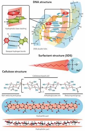


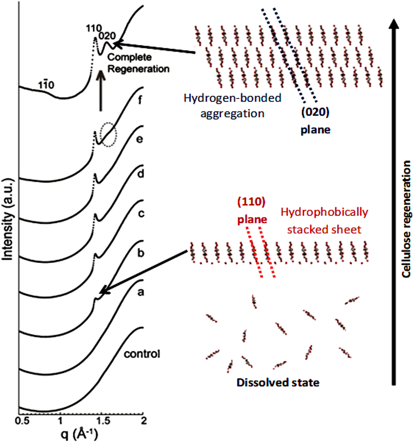


 Open access