


Introduction
Irrigation is a climate-resilient farming practice that mitigates crop damage from weather shocks (Smith and Edwards Reference Smith and Edwards2021; Tack et al. Reference Tack, Barkley and Hendricks2017; Troy et al. Reference Troy, Kipgen and Pal2015). In the United States, irrigation has traditionally been concentrated in the arid West, where precipitation is insufficient to meet crop water requirements. However, increasing water stress poses significant challenges to the long-term sustainability of irrigation-based agricultural systems (Deines et al. Reference Deines, Schipanski, Golden, Zipper, Nozari, Rottler, Guerrero and Sharda2020; Mrad et al. Reference Mrad, Katul, Levia, Guswa, Boyer, Bruen, Carlyle-Moses, Coyte, Creed, Van De Giesen, Grasso, Hannah, Hudson, Humphrey, Iida, Jackson, Kumagai, Llorens, Michalzik, Nanko, Peters, Selker, Tetzlaff, Zalewski and Scanlon2020). In contrast, the Eastern United States – characterized by a more humid climate and variable rainfall – has relied on precipitation, with producers increasingly adopting supplemental irrigation during critical crop growth stages (Mullen et al. Reference Mullen, Yu and Hoogenboom2009). In addition, the relative abundance of water for irrigation in the East offers new opportunities to expand irrigated agriculture and potentially shift the focus of irrigation development (Mehta et al. Reference Mehta, Siebert, Kummu, Deng, Ali, Marston, Xie and Davis2024).
The Southeast is one of the fastest-growing regions for irrigation adoption in the U.S. (Hrozencik and Aillery Reference Hrozencik and Aillery2022; Reidmiller et al. Reference Reidmiller, Avery, Easterling, Kunkel, Lewis, Maycock and Stewart2017), with South Carolina serving as a notable example. Between 2002 and 2022, irrigated agricultural land in South Carolina increased by 25%, adding 20,000 irrigated acres across its four major crops such as corn, cotton, peanuts and soybeans. However, despite the region’s potential for sustainable irrigation growth (Mehta et al. Reference Mehta, Siebert, Kummu, Deng, Ali, Marston, Xie and Davis2024; Rosa et al. Reference Rosa, Chiarelli, Sangiorgio, Beltran-Peña, Rulli, D’Odorico and Fung2020), adoption rates in the Southeast remain modest (Cooley and Smith Reference Cooley and Smith2022).
Farmers’ reliance on traditional farming practices can lead to inertia, slowing the adoption rate of new irrigation technologies (Perry et al. Reference Perry, Hennessy and Moschini2022). Therefore, identifying the factors that drive irrigation adoption decisions is crucial for policymakers, particularly as droughts are projected to increase in frequency (Strzepek et al. Reference Strzepek, Yohe, Neumann and Boehlert2010). This paper estimates the role of peer effects in shaping farmers’ decisions to adopt irrigation in South Carolina, using a unique parcel-level dataset on irrigation withdrawals collected annually by the South Carolina Department of Environmental Services (SCDES).
We argue that social interaction and social learning are two key mechanisms through which peer effects influence irrigation adoption in South Carolina. Social interaction refers to situations in which an individual’s benefit from taking an action increases when others take the same action, independent of any information exchange or learning (Cooper and Rege Reference Cooper and Rege2011; Lahno and Serra-Garcia Reference Lahno and Serra-Garcia2015). We use the number of peer irrigators to measure peers’ choices that may induce social interaction. This mechanism has been documented in irrigation adoption in arid agricultural systems such as Kansas (Sampson and Perry Reference Sampson and Perry2019b). In contrast, social learning could potentially play an important role in South Carolina. Because irrigation is typically used as a supplement to rainfall rather than as a year-round practice, farmers may differ in their understanding of the costs and benefits associated with adopting irrigation. Social learning occurs when individuals acquire information about the value of an action by observing the outcomes experienced by peers (Cooper and Rege Reference Cooper and Rege2011). For instance, a farmer may delay adoption until they observe clear evidence that irrigation has improved yields or reduced risk for their peers. We use peers’ water use as a measure of the potential value of irrigation among irrigators. Opportunities for learning are likely to be greater during drought conditions, when increased pumping makes the value of irrigation more visible and salient.
There are three common sources of endogeneity that make the identification of peer effects challenging: self-selection of peer group, correlated unobservables, and simultaneity (i.e., reflection) (Bollinger and Gillingham Reference Bollinger and Gillingham2012; Manski Reference Manski1993b). To mitigate bias from self-selection we control for various contextual factors, such as farm characteristics, crop type, weather conditions that could drive irrigation adoption (Carey and Zilberman Reference Carey and Zilberman2002; Hendricks and Peterson Reference Hendricks and Peterson2012; Schoengold et al. Reference Schoengold, Sunding and Moreno2006; Smith et al. Reference Smith, Andersson, Cody, Cox and Ficklin2017). Additionally, to address bias from correlated unobservables, we incorporate a rich set of fixed effects to account for unobserved factors that may simultaneously affect both individual farmers and their peers. Finally, to reduce reflection bias, we define peer effect using the installed base – the cumulative count of peer irrigators up to the previous year. This approach ensures that only past irrigation decisions by peers can influence current adoption decisions, eliminating reverse causality (Bollinger and Gillingham Reference Bollinger and Gillingham2012).
Our results provide evidence that both mechanisms – social interaction and social learning – can be relevant to irrigation adoption decisions among farmers who eventually adopt irrigation. Specifically, each additional peer irrigator increases the probability of adoption by 0.4 percentage points. We also find evidence of peer influence under conditions that enhance opportunities for learning about the value of irrigation. A 100 million gallon increase in peer irrigation water use is associated with a 0.3 percentage point increase in the probability of adoption. This finding suggests that as peers’ pumping increases – such as during drought conditions – the benefits of irrigation become more visible, thereby facilitating social learning and accelerating adoption.
Peer effects have gained growing attention as a key factor influencing the adoption of agricultural practices (Burlig and Stevens Reference Burlig and Stevens2023; Che et al. Reference Che, Feng and Hennessy2022; Mart nez et al. Reference Martínez, Maia and Garcia2022). In the context of irrigation technology adoption, existing evidence highlights the significant role of peer influences in acquiring groundwater rights and adopting water-saving irrigation technologies in Kansas (Sampson and Perry, Reference Sampson and Perry2019b,a). Building on this body of research, this study examines peer effects on irrigation adoption with a particular focus on the Southeastern United States. Our study also contributes to the existing literature on irrigation adoption (Carey and Zilberman Reference Carey and Zilberman2002; Sampson and Perry Reference Sampson and Perry2019b), social interaction (Sampson and Perry Reference Sampson and Perry2019b), and social learning (Burlig and Stevens Reference Burlig and Stevens2023; Erev and Roth Reference Erev and Roth2014; Foster and Rosenzweig Reference Foster and Rosenzweig1995), by examining the role of peer effect in shaping irrigation decisions. Unlike much of the existing research, which has predominantly examined irrigation practices in the arid Western U.S., this study focuses on a less-studied region, providing new insights into irrigation dynamics in the East.
Background
Irrigation trends and development in South Carolina
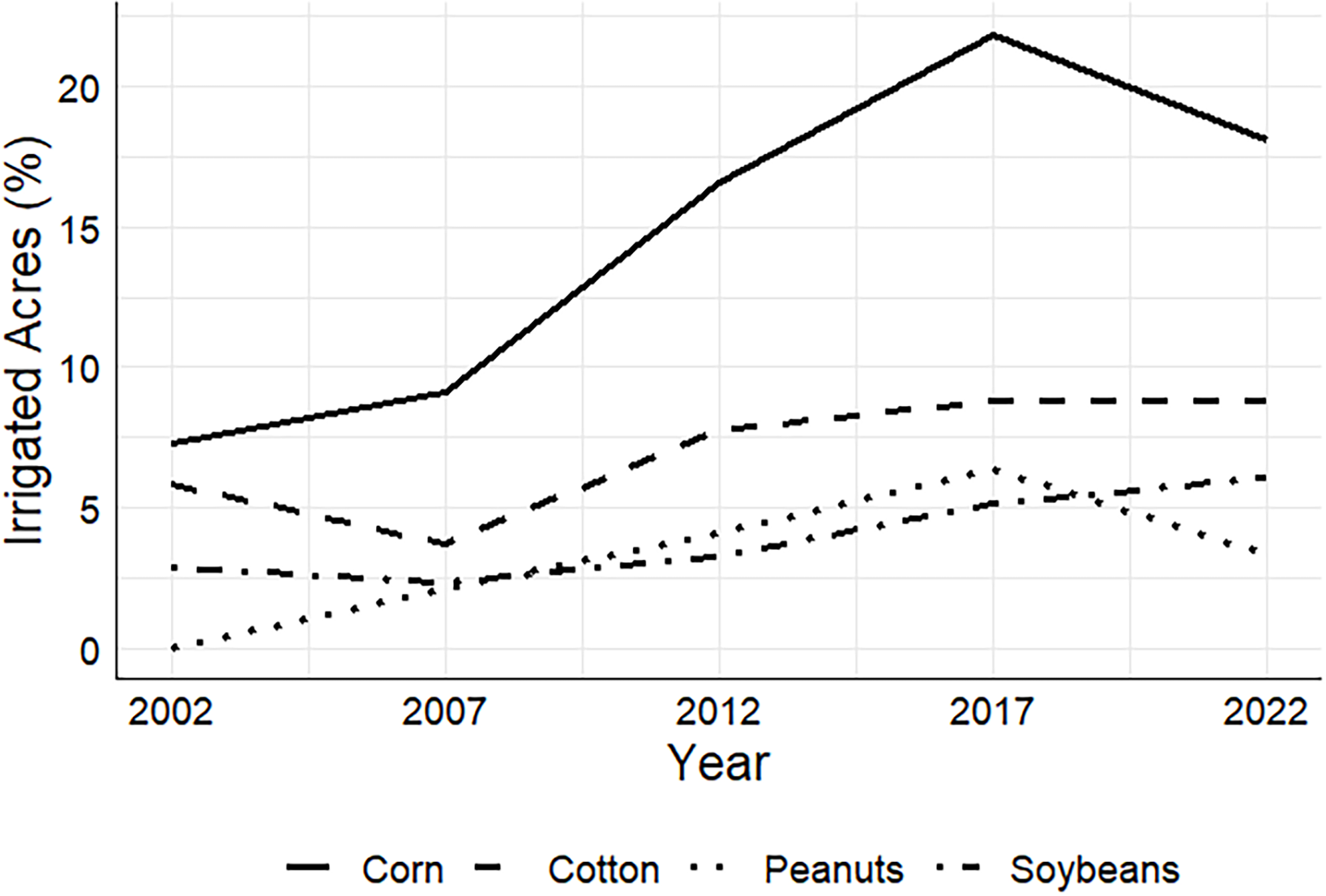
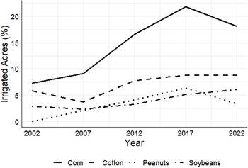
While irrigated land has decreased in the Western U.S. over the past two decades, the Eastern region has seen a significant expansion in irrigation practices (Hrozencik and Aillery Reference Hrozencik and Aillery2022; Xie and Lark Reference Xie and Lark2021). In South Carolina, this trend is particularly evident, with a significant increase in the irrigated acreage of major crops across the state. As Figure 1 shows, the percentage of irrigated corn acreage relative to the total harvested corn acres increased from 7.3% in 2002 to 18.1% in 2022. Similar upward trends in irrigation are observed for other crops, although to a lesser extent. For cotton, the percentage of irrigated harvested acres increased from 5.8% in 2002 to 8.8%, for peanuts from 0% to 3.3%, and for soybeans from 2.9% to 6.1%.
Trends in irrigated acreages by crops in South Carolina. Notes: The percentage of irrigated acres for each crop is calculated by dividing the number of irrigated harvested acres by the total harvested acres for that crop.
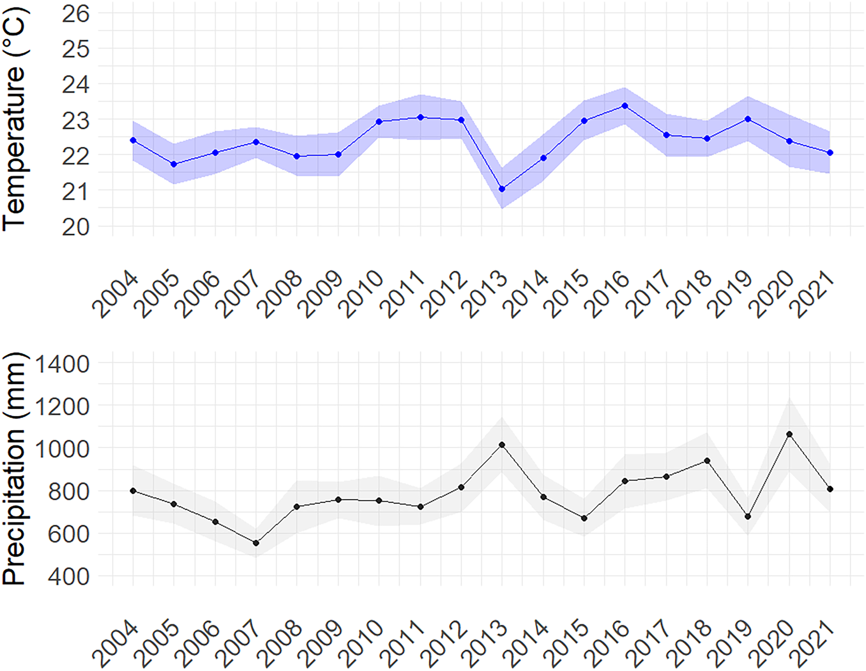
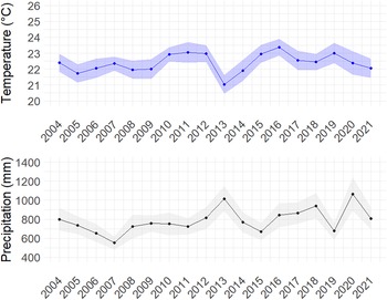
South Carolina’s climate is characterized by moderate temperatures and abundant rainfall throughout the year, creating generally favorable conditions for agricultural production. The state has received an average annual precipitation of 787 mm since 2004 (Figure 2), with an average temperature of 22.4C. This relatively high level of precipitation is a key factor in understanding the growing demand for irrigation in South Carolina given that the drivers of irrigation adoption may differ from those in drier states like Kansas, where annual precipitation is nearly half (approximately 416 mm).
Average growing season temperature and precipitation in South Carolina. Notes: In the upper panel, the solid line is the average growing season temperature computed by daily temperature at the irrigation permit sites during the growing seasons from March to September each year. The shaded areas show one standard deviation from the mean. In the bottom panel, the solid line shows the average precipitation computed by cumulative annual precipitation across irrigation permit sites during the growing seasons from March to September each year. The shaded areas represent one standard deviation from the mean.
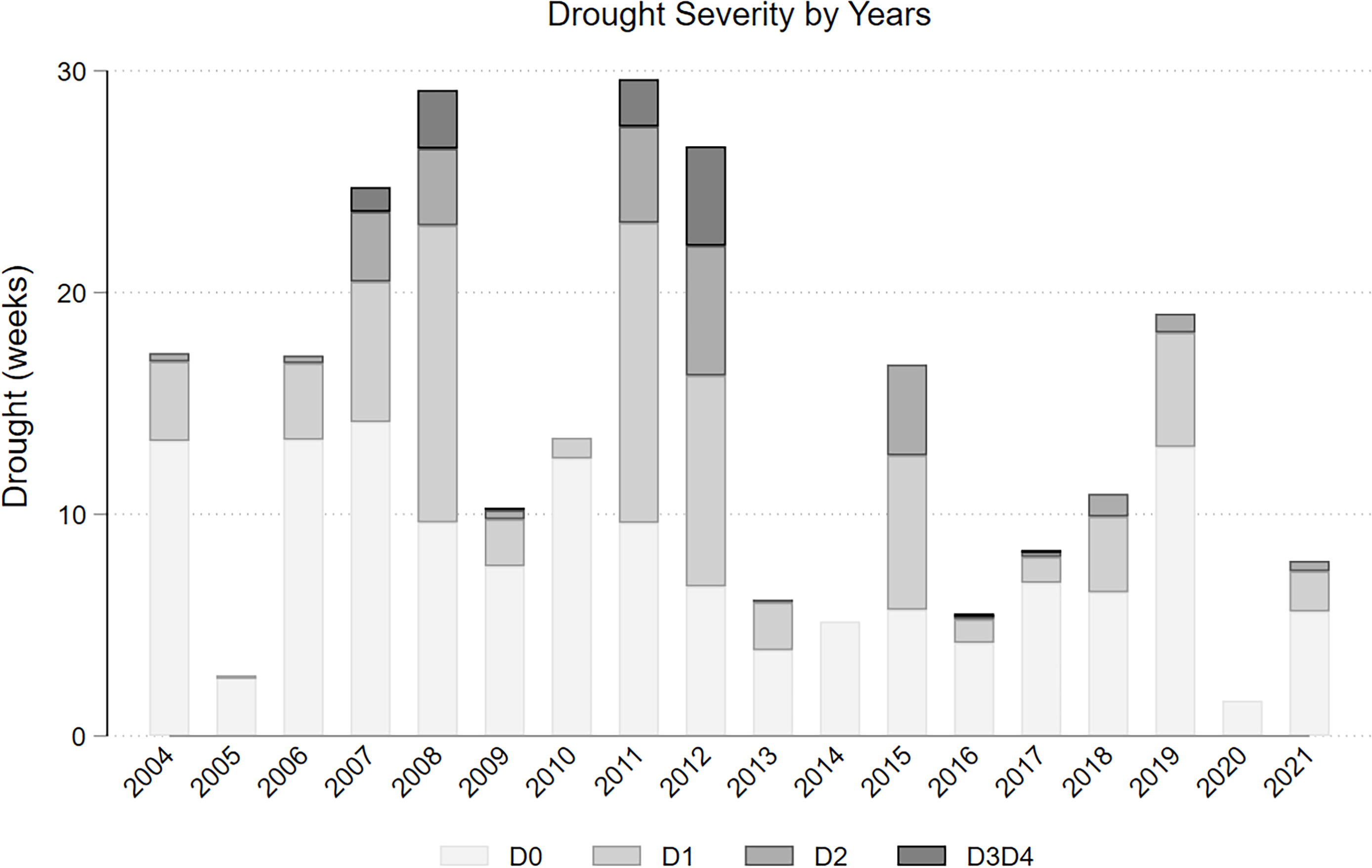
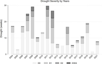
Although South Carolina generally receives adequate rainfall, it also experiences periodic droughts of varying severity and duration. Figure 3 illustrates drought conditions at irrigation permit sites across the state from 2004 to 2021. The figure presents the annual mean number of drought weeks at each severity level, ranging from Abnormally Dry (D0) to Exceptional Drought (D4), as defined by the U.S. Drought Monitor. Although the state generally experiences milder droughts, the duration and intensity of droughts vary substantially from year to year. The most severe drought events occurred in 2007, 2008, 2011, and 2012.
Drought severity in South Carolina. Notes: Each shade represents the annual average number of drought weeks across irrigation permit sites for the four drought severity categories. These categories, defined by the U.S. Drought Monitor, include Abnormally Dry (D0, lightest gray), Moderate Drought (D1, second lightest gray), Severe Drought (D2, darker gray), and Extreme/Exceptional Drought (D3 + D4, darkest gray). The bars are stacked to represent the total average number of drought weeks per year.
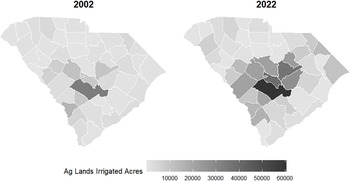
Over the past two decades, South Carolina has experienced significant growth in irrigation. Figure 4 shows the spatial distribution of irrigated agricultural land. Irrigation is primarily concentrated in the central regions and is unevenly distributed across counties, highlighting substantial regional heterogeneity in adoption patterns.
Spatial distribution of irrigated acres by county in 2002 and 2022. Notes: The map on the left shows the total irrigated land by county in 2002, while the map on the right shows the same for 2022. Darker gray shades indicate a higher concentration of irrigated land in each county. (Source: USDA NASS, Census of Agriculture).
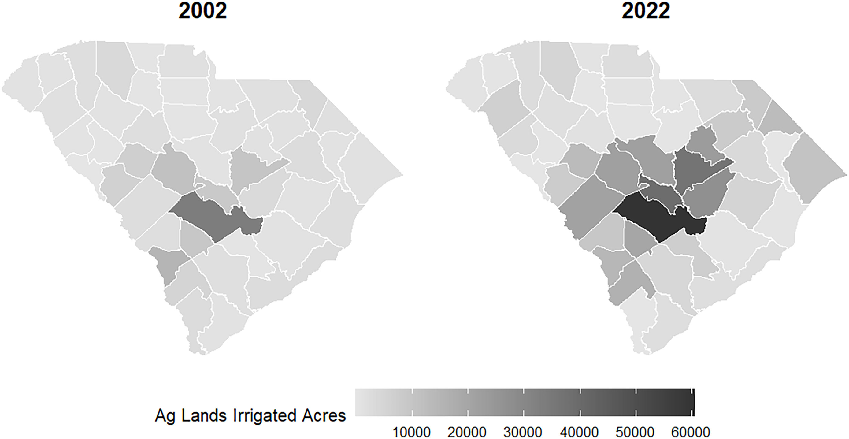
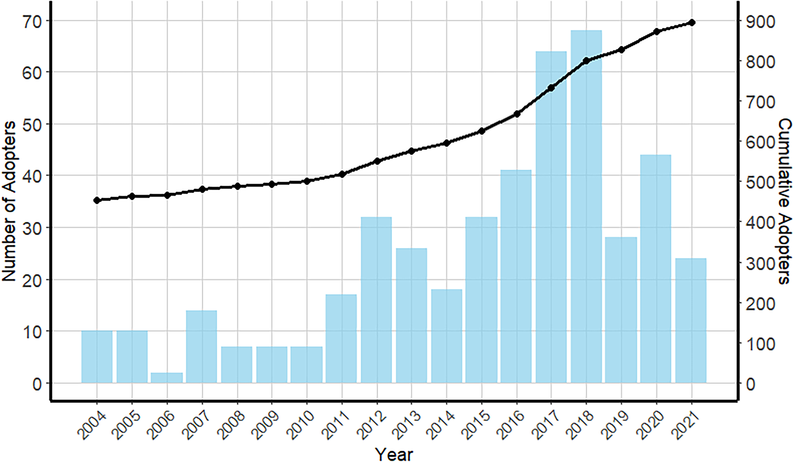
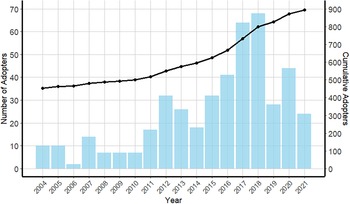
Figure 5 presents the trend in irrigation adoption in South Carolina. The top panel shows the annual number of new irrigation adopters between 2004 and 2021, while the bottom panel displays the cumulative number of adoptions since 1983, when South Carolina’s water withdrawal reporting rule was established. Prior to 2004, there were 444 irrigation permits. Adoption increased significantly from 2004 to 2021, nearly doubling the cumulative total. This surge in adoption may be attributed to the severe droughts of 2011, as indicated by the weather and drought patterns in Figures 2 and 3, or it could reflect farmers’ adaptive strategies in response to adverse weather, informed by past experiences. Alternatively, the increase could also be influenced by peer effects.
Trend of irrigation adoption in South Carolina. Notes: The bars show the number of annual irrigation adoptions from 2004 to 2021, and the solid line plots the cumulative number of adoptions by aggregating the annual figures in the top panel. The cumulative count includes 444 existing permit holders who adopted prior to 2004.
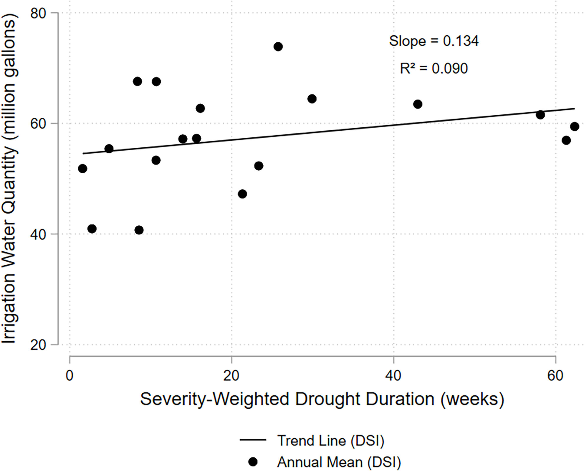
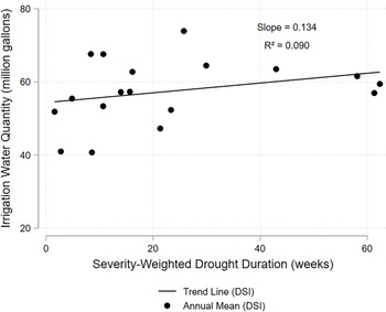
In South Carolina, irrigation is typically used as a supplement to rainfall rather than as a continuous, year-round practice, so water use tends to increase during drought periods. Figure 6 shows the relationship between drought conditions – measured by drought durations weighted by severity levels – and the corresponding irrigation groundwater usage, using annual averages from 2004 to 2021. In this context, peers’ irrigation water use can provide valuable information that influences a farmer’s decision to adopt irrigation.
Relationship between drought duration and irrigation water usage. Notes: This figure shows the annual number of drought weeks, weighted by drought severity categories (D0 to D4), where the weights assigned to each category are: D0 = 1, D1 = 2, D2 = 3, D3 = 4, and D4 = 5, following the Drought Severity and Coverage Index methodology (Akyuz, Reference Akyuz2017). These weighted values are plotted alongside the corresponding annual means of irrigation water usage (in million gallons) for each year from 2004 to 2021. Trend lines are included to illustrate the positive relationship between severity weighted drought durations and irrigation water usage.
Surface water has traditionally been the primary source of irrigation, but in recent years, groundwater has become increasingly dominant. Currently, 96% of new irrigation adopters rely on groundwater, while only 4% use surface water. As a result, irrigated farms are largely concentrated in regions where key aquifers are located, primarily east of the Fall Line, as shown in figure A1 in Supplementary Appendix A2. This area, known as the Coastal Plain, overlays the Atlantic Coastal Plain (ACP) aquifer system (Campbell et al. Reference Campbell, Petkewich, Coes and Fine2012). The ACP system consists of multiple layers of confined aquifers, with unconfined aquifers situated on top, each separated by impermeable materials. Between 2004 and 2021, 12 confined aquifers have been used for irrigation in South Carolina. More detailed information on these aquifers can be found in Supplementary Appendix A2.
Groundwater withdrawal regulation and reporting
South Carolina, as well as the rest of the states in the East of U.S., is governed by the riparian doctrine, in which water allocations are tied to the holding of land adjacent to a water source. However, South Carolina’s water use and reporting regulations have undergone substantial changes over time (Nix and Rad Reference Nix and Rad2022). Some of these changes are described next.
The South Carolina Groundwater Use Act was passed in 1969, establishing reporting requirements for groundwater withdrawals greater than or equal to 100,000 gallons on any day located within a Capacity Use Area (CUA). In 1993, amendments to the South Carolina Water Resources Planning and Coordination Act led to the dissolution of the South Carolina Water Resources Commission (Gellici Reference Gellici2011). Subsequently, its responsibilities were divided between two new entities: the South Carolina Department of Health and Environmental Control (SCDHEC), tasked with enforcing water regulations, and the South Carolina Department of Natural Resources, which leads water planning.Footnote 1 A mandatory reporting threshold of more than three million gallons (MG) in any one month was implemented in 2000 (Wachob et al. Reference Wachob, Park and Newcome2009). Lastly, in 2010, the South Carolina Surface Water Withdrawal, Permitting Use, and Reporting Act was passed and established a change in the South Carolina’s water law from riparian water rights to a regulated riparianism system (Taylor Reference Taylor2018).
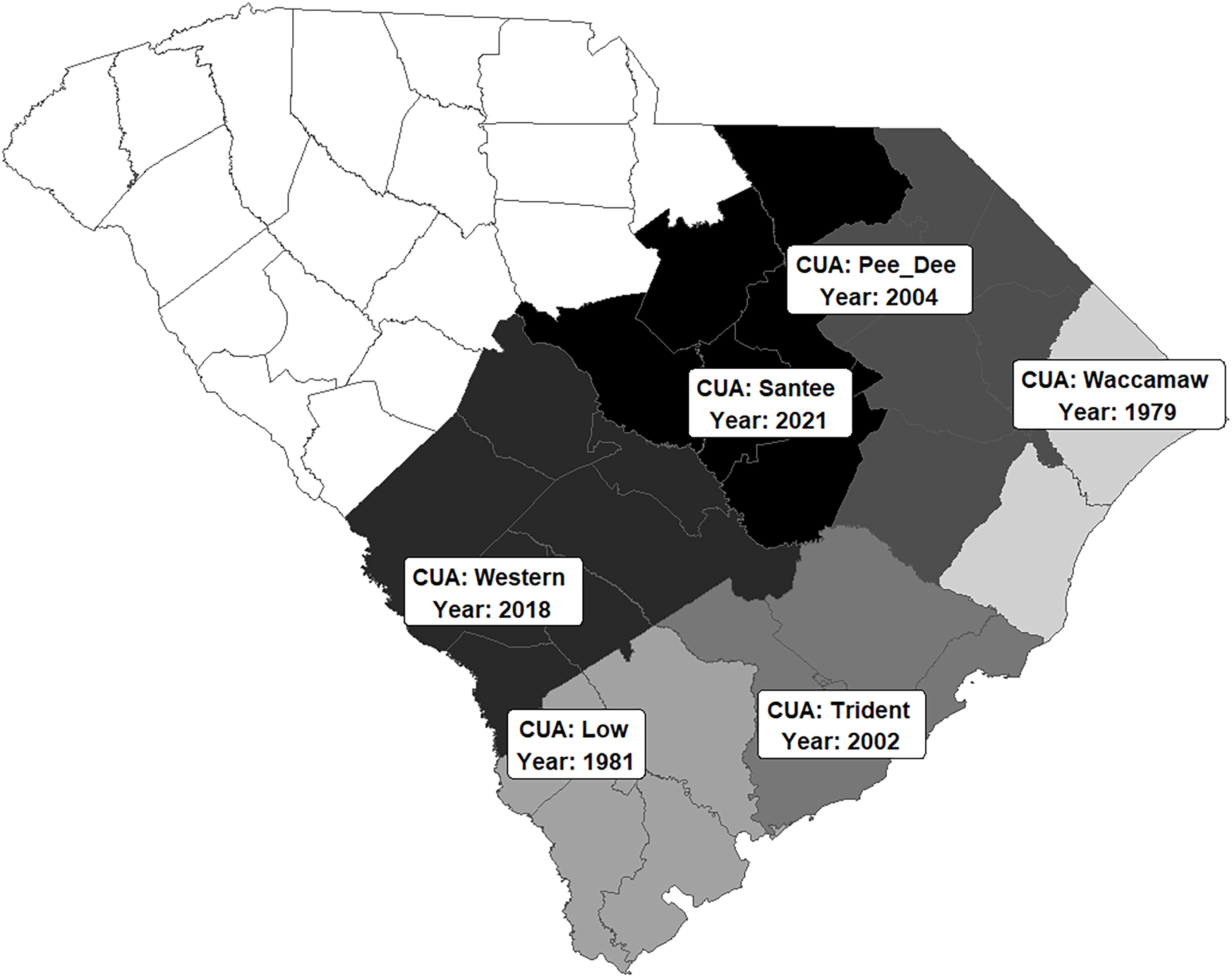
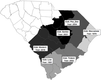
CUAs have been established over time to improve the effectiveness of monitoring and managing the use of aquifers across the state. There are currently six CUAs in place and the designations of CUA were initiated around coastal counties (Figure 7). The first CUA created was Waccamaw (1979) followed by Lowcountry (1981 and expanded in 2008), Trident (2002), Pee Dee (2004), Western (2018), and finally, Santee Lynches (2021).
The capacity use areas (CUA) in South Carolina. Notes: The shading indicates the timing of CUA designations. Lighter shades represent the three earlier-designated CUAs (Waccamaw, Low, and Trident), located near the coastal regions. Darker shades correspond to the later-designated CUAs (Pee Dee, Western, and Santee Lynches).
The location of the groundwater users determines if they need a permit to pump water for irrigation. Groundwater users who are located within a CUA are required to request a permit to construct and/or operate any well which will use over three million gallons in any one month (SCDES 2006).Footnote 2 Moreover, users outside CUAs need to register wells using over three million gallons per month. Statewide, all registered and permitted groundwater withdrawers must report their annual water use to the SCDES.Footnote 3
Permits for usage are subject to review and renewal every 5 years, and wells must shut down if they are no longer serving a beneficial purpose (SCDES 2006). However, non-compliance with these regulations does not necessarily result in immediate permit or registration revocation. There is typically some flexibility in maintaining permit status, even if water withdrawal is below the claimed volumes.
Data
The data used for our estimation are drawn from several sources at the finest resolution possible. Irrigation adoption information is obtained from the SCDES’s withdrawal data from 1983 to 2021. To evaluate new adoption, we use information on the first time a user reports withdrawals as a new permit is issued to that user.Footnote 4
The initial dataset includes 1,003 permits and 3,034 wells registered for irrigation water use. After removing data without spatial information, we are left with 955 permits associated with 2,828 wells. The difference between the number of permits and wells indicates that some permits cover multiple wells. Furthermore, permits are not always uniquely identified because some farmers hold multiple permits. Multiple wells and permits can introduce bias in measuring peer effects, as multi-permits holders’ decisions are not independent (Sampson and Perry Reference Sampson and Perry2019b). To avoid this issue, we create a unique match between each permit and well. As a result, our final dataset includes 451 permits with distinct corresponding well information. Detailed descriptions of our data processing methods for achieving unique permit identifications are provided in Supplementary Appendix A1. Lastly, in our sample, once a farmer adopts irrigation, they do not revert to dryland farming. We follow Sampson and Perry (Reference Sampson and Perry2019b) to code the binary dependent variable after irrigation adoption, and, consequently, observations from years following the adoption of irrigation are excluded from the analysis.
We also identify the water amount associated with each unique permit by assigning representative water usage to each permit holder. Representative water usage refers to the amount of water associated with each representative well.Footnote 5 To calculate this, we aggregate the total water usage from all wells linked to a given permit for each year. In this way, the water amount assigned to a permit reflects usage from all wells under that permit, not just from the representative well. Similarly, when multiple permits are held by the same entity, we calculate the total water usage by aggregating across those permits. This approach enables us to assign a consistent and representative annual water usage value to each uniquely identified permit in our study.
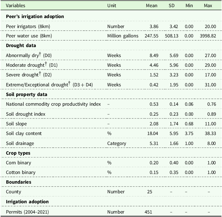
We compile a variety of data that may influence irrigation adoption decisions, including weather conditions, soil characteristics and crop type. Table 1 presents the summary statistics for the key variables included in the empirical model.
Summary statistics

Note: †indicates one-year lag variable.
Soil characteristics are obtained from the USDA NRCS (Natural Resources Conservation Service) gSSURGO dataset. We include the National Commodity Crop Productivity Index (NCCPI) and drought vulnerability index to examine the soil productivity factors. We also include other soil characteristics described next. Soil slope is defined as the difference in elevation between two points and reflects the degree of soil erosion. Soil clay content are determined by the particle sizes, which affect the degree of water-holding capacity. Eight drainage types define soil drainage data, from very poor to excellent drainage.Footnote 6
Peer effects and identification concerns
The influence of peer irrigators on a farmer’s decision to adopt irrigation can operate through two main distinct mechanisms: social interaction and social learning. Social interaction refers to situations in which an individual’s utility from taking an action increases when others also take that action, regardless of whether information is exchanged or learning occurs (Cooper and Rege Reference Cooper and Rege2011; Lahno and Serra-Garcia Reference Lahno and Serra-Garcia2015). For example, a farmer may install irrigation because his neighbors have done so, even without detailed information of the costs and benefits. In contrast, social learning occurs when individuals acquire information about the value and effectiveness of an action by observing the behavior and outcomes experienced by others (Banerjee Reference Banerjee1992; Cooper and Rege Reference Cooper and Rege2011). In this case, a farmer may need to receive information that irrigation has improved neighbors’ crop yields or reduced production risks before deciding to adopt similar practices.
We assume that the benefits of adopting irrigation are uncertain for farmers prior to adoption. Farmers may form prior beliefs about these potential benefits based on observable factors related to irrigation installation. These beliefs can then be updated through opportunities to learn from peers who have already adopted irrigation (Genius et al. Reference Genius, Koundouri, Nauges and Tzouvelekas2014; Moretti Reference Moretti2011). Such belief updating primarily occurs through social learning, as farmers receive feedback – either directly or through observation – from neighboring adopters. We argue that in regions like the Eastern U.S., where irrigation serves as a supplemental input, peer effects on irrigation adoption may operate not only through social interaction but also, and perhaps more importantly, through social learning. The potential for social learning may be further enhanced during drought conditions, when the value of irrigation becomes even more apparent. In such periods of water stress, farmers are more likely to observe and internalize the advantages of irrigation, increasing the likelihood of adoption.
There are several challenges common to empirical analysis of social mechanisms. The first one refers to the definition of the peer group. The SCDES withdrawal data provide information about the water permit’s location, but no information about who their peers are is available. We combine the location and irrigation adoption information to define the adopter’s peer network based on geography (Bollinger et al. Reference Bollinger, Burkhardt and Gillingham2020; Sampson and Perry Reference Sampson and Perry2019a) rather than spatial proximity (Sampson and Perry Reference Sampson and Perry2019b; Towe and Lawley Reference Towe and Lawley2013). The intuition behind this definition is that irrigation systems are visible to peers so farmers are more likely to be exposed to information about irrigation practices when they are nearby. Additionally, farms in South Carolina differ in field sizes and the distances between them. Consequently, using spatial proximity (e.g., the nearest 13 neighbors) to define peer groups may be problematic if the selected farms are not sufficiently close to one other to provide meaningful information about irrigation practices.
We create a buffer around each water permit to define peer group as farmers who eventually adopt irrigation within a 8-km radius of each individual farmer in our dataset. To address uncertainty regarding the distance farmers consider relevant for peer influence, we vary buffer sizes from 3 to 20 km as part of our robustness check in Section (Robustness checks). A graphical illustration of a buffer used to compute the installed base is provided in figure A3, Supplementary Appendix, section A2. However, this definition of peer group does not account for other social interactions that occur outside the buffer. For instance, farmers may interact with peers in cooperatives, extension centers, or input stores. Therefore, our definition of a peer group can be considered as the minimum threshold for social interaction that influences irrigation adoption decisions.
There are two main types of effects that explain why members of the same group could behave similarly (Bollinger and Gillingham Reference Bollinger and Gillingham2012; Manski Reference Manski1993b). The first is contextual effects, which occur when the behavior of individuals in a group is influenced by exogenous characteristics of the group. In our context, there is an exogenous effect if farmers’ irrigation adoption decisions vary with soil characteristics, weather, or crop choices. In contrast, endogenous effects (i.e., peer effects) occur when an individual’s behavior is directly influenced by the actions of other group members (Burlig and Stevens Reference Burlig and Stevens2023; Di Falco et al. Reference Di Falco, Doku and Mahajan2020). An example of an endogenous effect is if a farmer’s decision to adopt irrigation is influenced by exchanging information about the returns to irrigation with their peers.
From a policy perspective, it is important to disentangle endogenous peer effects from contextual effects due to different policy implications (Manski Reference Manski1993b). However, there are three common sources of endogeneity that make the identification of peer effects challenging (Bollinger and Gillingham Reference Bollinger and Gillingham2012; Manski Reference Manski1993b): self-selection of peer group, correlated unobservables, and simultaneity (i.e., reflection). The first is self-selection of the peer group (i.e., homophily), which can occur when individuals can choose their peer group. In our context, farmers with similar preferences may sort into a certain rural area, or more progressive farmers might form a group where everyone is inclined towards adopting new technologies. Thus, this self-selection can bias the estimation of peer effects because the decision to adopt irrigation is not only due to peer influence but also to pre-existing similarities.
Various contextual factors, such as soil characteristics, crop type, and weather could influence irrigation adoption. We control for these factors by including a rich set of covariates. However, many other factors (e.g., farmers’ preferences, policy changes, macroeconomic shocks) may affect both individual farmers and peers but are unobserved by the researcher. Failing to control these unobserved factors makes isolating the actual peer effect difficult, leading to the second source of endogeneity, correlated unobservables.
A common approach to addressing the self-selection of peers and correlated unobservables is to include random or fixed effects (Bollinger and Gillingham Reference Bollinger and Gillingham2012; Nair et al. Reference Nair, Manchanda and Bhatia2010; Sampson and Perry Reference Sampson and Perry2019a). We include several fixed effects to account for unobserved heterogeneity. Year fixed effects are included to control for time-varying unobserved factors, while county fixed effects account for time-invariant spatial differences across counties. Lastly, we further control for unobserved largely spread shocks, especially spatial-temporal shocks by using the common correlated effect (CCE) at the state level as suggested by Sampson and Perry (Reference Sampson and Perry2019b). The CCE is defined as
 $\mathop \sum \nolimits_i {d_{it}}/{I_t}$
, a ratio between
$\mathop \sum \nolimits_i {d_{it}}/{I_t}$
, a ratio between
 ${d_{it}}$
(1 if
${d_{it}}$
(1 if
 $i$
adopts irrigation in time
$i$
adopts irrigation in time
 $t$
) and
$t$
) and
 ${I_t}$
(the number of eventual adopters in time
${I_t}$
(the number of eventual adopters in time
 $t$
that have not yet adopted. Thus, CCE aims to control for unexpected adoption patterns at the state levels.
$t$
that have not yet adopted. Thus, CCE aims to control for unexpected adoption patterns at the state levels.
The last identification concern relates to the simultaneity or reflection problem, which occurs when the decision of one farmer to adopt irrigation might influence, and be influenced by, the decisions of their peers simultaneously. The reflection problem creates a challenge in distinguishing whether a farmer’s decision is influencing their peers or vice versa. This issue is common when estimating peer effects using observational data and can introduce bias if not addressed (Bollinger and Gillingham Reference Bollinger and Gillingham2012; Manski Reference Manski1993a). Similar to previous studies (Sampson and Perry Reference Sampson and Perry2019b; Sampson and Perry Reference Sampson and Perry2019a), we expect a low impact from the reflection problem due to the lag between when a farmer observes their peers obtaining a positive return from irrigation and when he decides to install irrigation. Thus, we follow the approach proposed by Bollinger and Gillingham (Reference Bollinger and Gillingham2012) to define installed base as the variable measuring peer effects. The installed base is the cumulative number of adopters up to the previous calendar year within a peer group. We calculate the installed base using the following formula:
 $${b_{{z_i}t}} = \mathop \sum \limits_{\tau = 1}^{t - 1} \,\mathop \sum \limits_{j = 1}^{{m_{{z_i}}}} \,{a_{j\tau }}.$$
where
 ${m_{{z_i}}}$
is the number of farmers within the peer group who eventually adopt, and
${m_{{z_i}}}$
is the number of farmers within the peer group who eventually adopt, and
 ${a_{j\tau }}$
is an indicator variable of adoption in year
${a_{j\tau }}$
is an indicator variable of adoption in year
 $\tau $
. The installed base of farmer
$\tau $
. The installed base of farmer
 $i$
in peer-group
$i$
in peer-group
 $z$
in year t (i.e.,
$z$
in year t (i.e.,
 ${b_{{z_i}t}}$
) reflects the stock of neighbors that have adopted irrigation at or before
${b_{{z_i}t}}$
) reflects the stock of neighbors that have adopted irrigation at or before
 $\left( {t - 1} \right)$
.
$\left( {t - 1} \right)$
.
Empirical model
This section describes the empirical model to estimate the peer effects on irrigation adoption. We observe each farmer
 $i$
over
$i$
over
 $t = 1, \ldots, {T_i}$
years, where
$t = 1, \ldots, {T_i}$
years, where
 ${T_i}$
represents the year in which farmer
${T_i}$
represents the year in which farmer
 $i$
decides to adopt irrigation
$i$
decides to adopt irrigation
 $\left( {{y_{it}} = 1} \right)$
. We assume that the adoption decision is based on a comparison of the anticipated profits from adopting irrigation,
$\left( {{y_{it}} = 1} \right)$
. We assume that the adoption decision is based on a comparison of the anticipated profits from adopting irrigation,
 ${\pi _{it}}\left( {{y_{it}} = 1} \right)$
, with the profits from not adopting,
${\pi _{it}}\left( {{y_{it}} = 1} \right)$
, with the profits from not adopting,
 ${\pi _{it}}\left( {{y_{it}} = 0} \right)$
. Thus, farmer
${\pi _{it}}\left( {{y_{it}} = 0} \right)$
. Thus, farmer
 $i$
chooses to adopt irrigation in year
$i$
chooses to adopt irrigation in year
 $t$
if
$t$
if
 ${\pi _{it}}\left( {{y_{it}} = 1} \right) \gt {\pi _{it}}\left( {{y_{it}} = 0} \right)$
.
${\pi _{it}}\left( {{y_{it}} = 1} \right) \gt {\pi _{it}}\left( {{y_{it}} = 0} \right)$
.
The profit function can be decomposed into two components – an observed part
 ${V_{it}}$
, and unobserved error term
${V_{it}}$
, and unobserved error term
 ${\varepsilon _{it}}$
:
${\varepsilon _{it}}$
:
 $${\pi _{it}} = {V_{it}} + {\varepsilon _{it}}$$
The observed part is further modeled as a function of the installed base, defined in Equation 1, as well as production-related characteristics:
 $${V_{it}} = {\beta _1}Pee{r_{i,t - 1}} + {\beta _2}Peer_{i,t - 1}^2 + \gamma {\rm{'}}{X_{i,t - 1}} + {\rm{\Psi '}}CC{E_t} + {\rm{\Phi '}}{Z_i} + {\eta _t} + {\mu _g},$$
where
 $Pee{r_{i,t - 1}}$
denotes either the number of neighboring farmers who had adopted irrigation by year
$Pee{r_{i,t - 1}}$
denotes either the number of neighboring farmers who had adopted irrigation by year
 $t - 1$
(i.e., installed base of farmer
$t - 1$
(i.e., installed base of farmer
 $i$
in year
$i$
in year
 $t$
), or the amount of irrigation water used by those neighboring farmers who had adopted irrigation by year
$t$
), or the amount of irrigation water used by those neighboring farmers who had adopted irrigation by year
 $t - 1$
.Footnote 7 We employ these two distinct measures of peer effects to explore the plausibility of the two potential mechanisms, social interaction and social learning, without attempting to compare their relative magnitudes. We use peers’ water use as a measure to the potential knowledge gains provided to those peers that are irrigating. To capture potential non-linearities in peer effects, we include the squared term of the peer variable
$t - 1$
.Footnote 7 We employ these two distinct measures of peer effects to explore the plausibility of the two potential mechanisms, social interaction and social learning, without attempting to compare their relative magnitudes. We use peers’ water use as a measure to the potential knowledge gains provided to those peers that are irrigating. To capture potential non-linearities in peer effects, we include the squared term of the peer variable
 $Pee{r_{i,t - 1}}$
.
$Pee{r_{i,t - 1}}$
.
 ${X_{i,t - 1}}$
represents a vector of time-varying drought conditions – measured as the number of weeks under each drought severity level (D0, D1, D2, and D3 + D4) at the location of individual irrigators in year
${X_{i,t - 1}}$
represents a vector of time-varying drought conditions – measured as the number of weeks under each drought severity level (D0, D1, D2, and D3 + D4) at the location of individual irrigators in year
 $t - 1$
.
$t - 1$
.
 $CC{E_t}$
represents common correlated effects at the state level.
$CC{E_t}$
represents common correlated effects at the state level.
 ${Z_i}$
contains time-invariant variables such as soil characteristics.
${Z_i}$
contains time-invariant variables such as soil characteristics.
 ${\eta _t}$
and
${\eta _t}$
and
 ${\mu _g}$
are temporal and spatial fixed effects.
${\mu _g}$
are temporal and spatial fixed effects.
 ${\beta _1}$
,
${\beta _1}$
,
 ${\beta _2}$
,
${\beta _2}$
,
 $\gamma $
,
$\gamma $
,
 ${\rm{\Psi }}$
,
${\rm{\Psi }}$
,
 ${\rm{\Phi }}$
indicate the parameters to be estimated.
${\rm{\Phi }}$
indicate the parameters to be estimated.
The probability of adopting irrigation can be estimated using a logit model within the random utility framework. Assuming that unobservable component
 ${\varepsilon _{it}}$
, in Equation 3, is IID and follows the Type I extreme value distribution, the probability of adopting irrigation is given by the logit expression:
${\varepsilon _{it}}$
, in Equation 3, is IID and follows the Type I extreme value distribution, the probability of adopting irrigation is given by the logit expression:
 $$Pr({y_{it}} = 1|{V_{it}}) = \Lambda \left[ {{V_{it}}} \right] = {{exp\left( {{V_{it}}} \right)} \over {1 + exp\left( {{V_{it}}} \right)}}$$
where
 ${\rm{\Lambda }}$
represents the logistic cumulative distribution function, which ensures that the probability lies within the range of 0 to 1. Equation 4 can be expressed in terms of the odds of adoption as
${\rm{\Lambda }}$
represents the logistic cumulative distribution function, which ensures that the probability lies within the range of 0 to 1. Equation 4 can be expressed in terms of the odds of adoption as
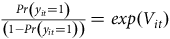 ${{Pr\left( {{y_{it}} = 1} \right)} \over {\left( {1 - Pr\left( {{y_{it}} = 1} \right)} \right)}} = exp\left( {{V_{it}}} \right)$
.
${{Pr\left( {{y_{it}} = 1} \right)} \over {\left( {1 - Pr\left( {{y_{it}} = 1} \right)} \right)}} = exp\left( {{V_{it}}} \right)$
.
Our primary goal is to estimate how changes in covariates affect the probability of irrigation adoption. To achieve this, we can estimate either the odds ratio (OR) or the marginal effects (ME). The odds ratio represents the ratio of the odds of irrigation adoption when a
 ${j^{th}}$
covariate (
${j^{th}}$
covariate (
 ${X_j}$
) is increased by one unit, and is expressed as
${X_j}$
) is increased by one unit, and is expressed as
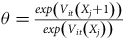 $\theta = {{exp\left( {{V_{it}}\left( {{X_j} + 1} \right)} \right)} \over {exp\left( {{V_{it}}\left( {{X_j}} \right)} \right)}}$
. When
$\theta = {{exp\left( {{V_{it}}\left( {{X_j} + 1} \right)} \right)} \over {exp\left( {{V_{it}}\left( {{X_j}} \right)} \right)}}$
. When
 ${V_{it}}$
is linear in the covariates, the odds ratio simplifies to
${V_{it}}$
is linear in the covariates, the odds ratio simplifies to
 $exp\left( {{\beta _j}} \right)$
. We use marginal effects to test peer effects, as they are easier to interpret in a non-linear logistic regression model. To estimate the marginal effect of the Peer variable in our specification, we use the following expression:
$exp\left( {{\beta _j}} \right)$
. We use marginal effects to test peer effects, as they are easier to interpret in a non-linear logistic regression model. To estimate the marginal effect of the Peer variable in our specification, we use the following expression:
 $${{\partial Pr\left( {{y_{it}} = 1} \right)} \over {\partial Pee{r_{i,t - 1}}}} = \Lambda '\left[ {{V_{it}}} \right] \cdot {{\partial {V_{it}}} \over {\partial Pee{r_{i,t - 1}}}}$$
The Average Marginal Effect (AME) is computed by first calculating the marginal effect for each observation in the sample, using the observed values of all covariates. The individual marginal effects are then averaged, providing a summary measure of the overall impact.
The odds ratio can be interpreted as the odds of adopting irrigation change with a one-unit increase in a variable. Thus, an odds ratio greater than one indicates the increasing likelihood of adoption, while less than one suggests a decreasing likelihood. In contrast, the AME measure the marginal change in the probability of adoption for each unit increase in a covariate, offering a direct interpretation of how covariates affect adoption probability.
Results
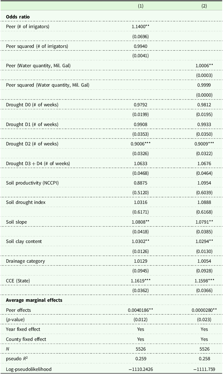
Table 2 presents the estimation results from the logistic regression. The table presents two columns corresponding to alternative model specifications of peer effect mechanisms. Column (1) uses Peer, the number of peer irrigators (i.e., the installed base), as the main explanatory variable – primarily capturing the social interaction mechanism. In contrast, column (2) uses peers’ water use as the key explanatory variable to capture the information channel through which social learning occurs. Peer Water Use is calculated as the sum of irrigation water used by the installed-base peers in the previous years. As such, the Peer Water Use reflects not only the number of peers but also their pumping behavior, which is likely influenced by annual weather conditions as farmers adjust irrigation to maximize crop revenue. Therefore, Peer Water Use captures the value of irrigation among peers in a given year, as observed by a given farmer – social learning mechanism.
Estimation results from logistic regression models
Notes: Odds ratios reported; standard errors in parentheses. Standard errors clustered by county. *
 $p \lt 0.1$
, **
$p \lt 0.1$
, **
 $p \lt 0.05$
, ***
$p \lt 0.05$
, ***
 $p \lt 0.01$
. Year and county fixed effects are included in all models. Drought variables are lagged by one year.
$p \lt 0.01$
. Year and county fixed effects are included in all models. Drought variables are lagged by one year.
We estimate two alternative specifications that separately capture social interaction (number of adopting peers) and social learning (peers’ water use). It is important to note that these specifications are not intended to determine which peer-effect mechanism dominates, because the peer variables are measured on different scales and their coefficients are not directly comparable across models. All models include year fixed effects and county fixed effects. Standard errors are clustered at the county level to account for heteroskedasticity and spatial correlation in unobserved errors. All peer variables are constructed based on the installed base within an 8 km radius buffer.
Our results in Column (1) of Table 2 show evidence of peer effects operating through the social interaction mechanism on irrigation adoption among farmers who adopt irrigation. Specifically, the estimated coefficients for Peer, along with the corresponding marginal effects, are positive and statistically significant. That is, one more peer irrigator increases the probability of irrigation adoption by about 0.4 percentage point. In addition, Column (2) provides some evidence of peer influence under conditions that enhance opportunities for learning about the value of irrigation. For instance, such opportunities are likely to be enhanced during drought conditions, when increased pumping by peers makes the benefits of irrigation more observable. Specifically, a 100 million gallon increase in peer irrigation water use is associated with a 0.3 percentage point increase in the probability of adoption. In both columns, the squared term of Peer is less than one, suggesting some evidence of diminishing peer effects. However, the estimates are not statistically significant.
We also report odds ratios in Table 2 to examine additional factors influencing irrigation adoption. In both columns, the odds ratios for milder droughts (D0–D2) are less than one, although only drought at the D2 level is statistically significant. This suggests that each additional week of drought at the D2 level in the previous year reduces the odds of irrigation adoption by about 10%. One possible explanation is that farmers may respond to moderate droughts by temporarily reducing crop acreage to limit production risks rather than investing in new irrigation systems. By contrast, under more severe droughts (D3–D4), the odds ratio exceeds one, indicating that farmers may be more likely to consider adoption during extreme or exceptional droughts. However, these effects are not statistically significant. Soil characteristics appear to play a role. For instance, steeper slopes are associated with greater odds of adopting irrigation – 7.9–8.1% increase in odds. Moreover, a 1% increase in clay content raises the odds of adoption by 2.9–3.0%.Footnote 8
Robustness checks
We conduct two robustness checks to assess the sensitivity of the estimation results. First, we estimate linear probability models as an alternative to logit models. In logistic regression, the estimation of marginal effects incorporates all parameters, which can result in biased estimates when multiple fixed effects are included – a phenomenon known as incidental parameters bias (Greene et al. Reference Greene, Han and Schmidt2002). To address this issue, we employ Ordinary Least Squares (OLS) regression using the same four model specifications as in Table 2.
The OLS regression results are presented in table A4 in Supplementary Appendix section A5. Consistent with the logistic regression results in Table 2, the average marginal peer effects in the OLS models are statistically significant in columns (1) and (2).
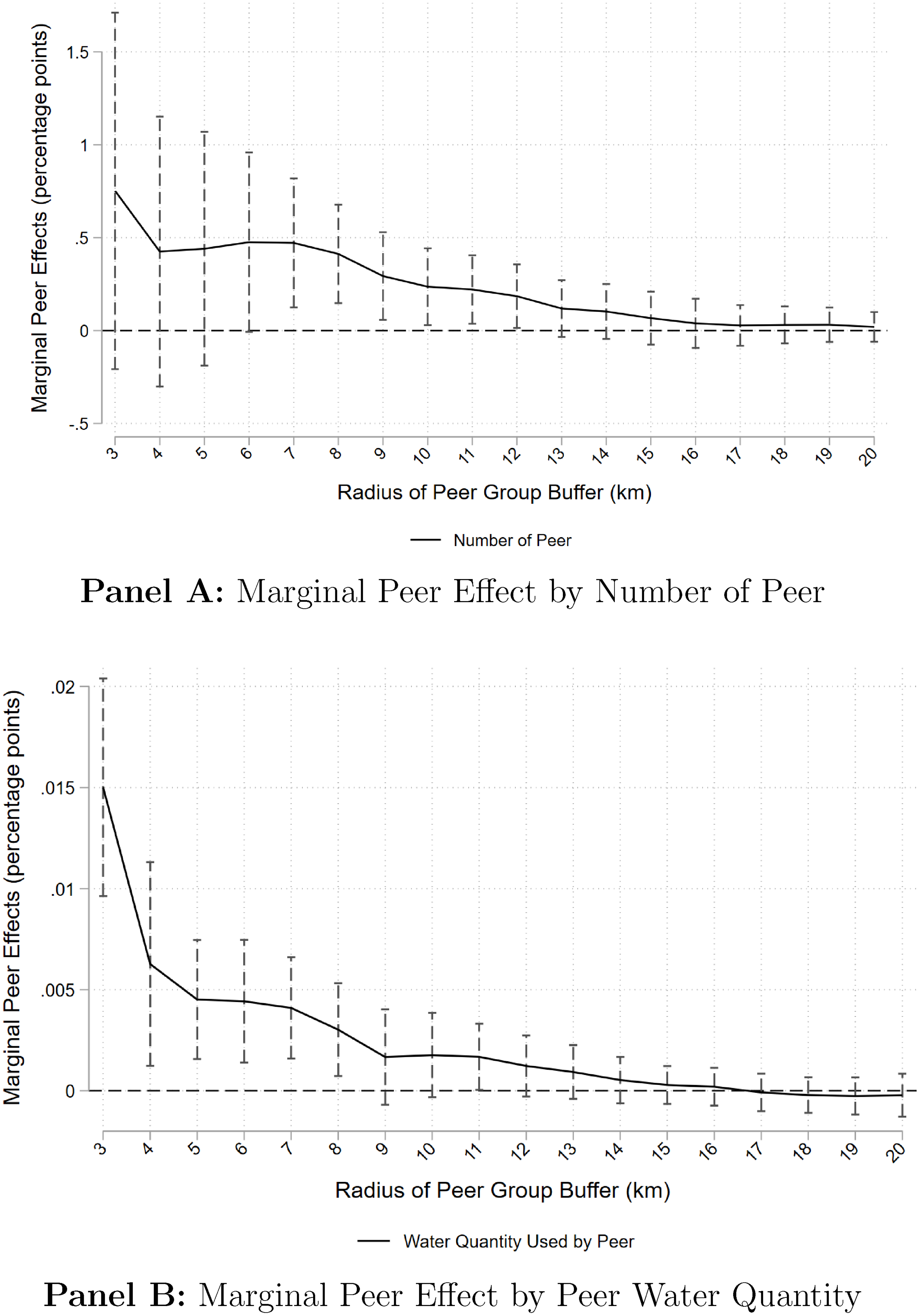
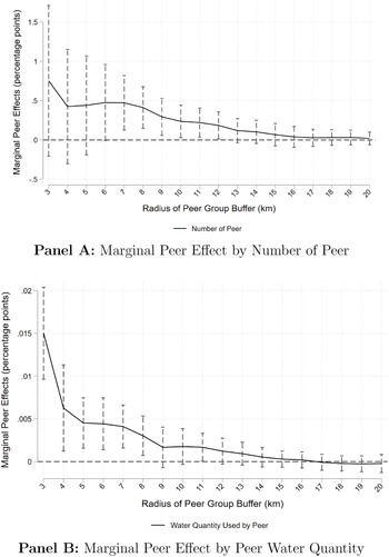
Our second robustness check examines whether estimates from our main model specification (using an 8 km radius definition of peer group) are sensitive to changes in peer group size. Figure 8 presents the estimated average marginal effects of the number of irrigators and peers’ water use in panels A and B, respectively. Each panel shows the average marginal peer effects for peer group sizes ranging from 3 km to 20 km. The results indicate that as the peer group size increases, the impact of peer effects generally diminishes across both mechanisms. However, the positive and statistically significant peer effect associated with peer numbers remains robust for most radii between 7 km and 11 km, while the peer effect associated with peer water use remains robust for most radii between 3 km and 8 km. Overall, these findings suggest that the peer effect remains generally consistent across varying peer group sizes.
Marginal Peer Effects by Peer Group Size. Panel A plots the estimated marginal effects of peer irrigation adoption (number of irrigators) for each peer group size, ranging from 3 km to 20 km. Panel B plots the estimated marginal effects of peer water use (water quantity) for each peer group size, ranging from 3 km to 20 km.
Discussion and conclusions
Agriculture is one of the sectors most vulnerable to climate change, with rising temperatures already leading to reduced crop yields (Lobell et al. Reference Lobell, Schlenker and Costa-Roberts2011; Ortiz-Bobea et al. Reference Ortiz-Bobea, Ault, Carrillo, Chambers and Lobell2021; Tack et al. Reference Tack, Barkley and Nalley2015). Irrigation adoption is often suggested as a potential adaptation practice to mitigate the risks associated with drought conditions, and expanding irrigation across rain-fed croplands could help to meet future global food demand (Rosa Reference Rosa2022). In the U.S., irrigated areas are increasing in the Midwest, the Mississippi Alluvial Plain, and the East Coast, while decreasing in hotspots such as the central and southern High Plains, southern Central Valley in California and Arizona (Xie and Lark Reference Xie and Lark2021), where irrigation has played a key role in the development of agriculture (Edwards and Smith Reference Edwards and Smith2018; Hornbeck and Keskin Reference Hornbeck and Keskin2014).
Despite the potential for sustainable irrigation expansion in the eastern U.S. (Mehta et al. Reference Mehta, Siebert, Kummu, Deng, Ali, Marston, Xie and Davis2024; Rosa et al. Reference Rosa, Chiarelli, Sangiorgio, Beltran-Peña, Rulli, D’Odorico and Fung2020), adoption rates remain low (Cooley and Smith Reference Cooley and Smith2022). For example, irrigated corn acres in South Carolina were 18% in 2022 – well below rates in Georgia (52%) and Florida (45%) (USDA 2025). In this context, understanding whether a farmer’s decision to adopt irrigation is influenced by the irrigation practices of their peers could improve the effectiveness of policies aimed at mitigating drought risks.
We find evidence that both a greater number of peer irrigators and higher water use by peers influence adoption decisions among farmers who adopt irrigation. Our results suggest that adoption increases as farmers observe more peer adopting irrigation – social interactions – and as peers’ pumping increases, such as during drought periods, when the benefits of irrigation become more visible and there are more opportunities to observe and learn the value of irrigation, facilitating social learning.
The evidence of peer effects presented in our paper aligns with the results reported among farmers in Kansas by Sampson and Perry (Reference Sampson and Perry2019b), who found peer effects of 0.25–0.41 percentage points depending on model specifications. This consistency between the two studies highlights the important role of peer influence through social interaction, despite several key contextual differences. Moreover, our study complements these previous results by providing evidence of the additional role of peer effects operating through social learning.
In Kansas, crop production relies heavily on groundwater irrigation as the primary source of water, whereas crop production in South Carolina depends predominantly on rainfall. Farmers in South Carolina receive nearly twice the annual rainfall of their counterparts in Kansas, with an average precipitation of 787 mm in South Carolina compared to 416 mm in Kansas. Therefore, irrigation in South Carolina primarily serves as a supplement to rainfall, rather than being a consistent, year-to-year source of water, which may offer minimal or no net economic benefit (Partridge et al. Reference Partridge, Winter, Kendall, Basso, Pei and Hyndman2023). However, our results are consistent with Sampson and Perry (Reference Sampson and Perry2019b), indicating that peer effects – measured by neighboring irrigators – are also an important driver of irrigation adoption in South Carolina.
Groundwater depletion–combined with the common-pool nature of the resource–can influence irrigation adoption decisions, as farmers may be concerned about overuse by their peers Sampson and Perry (Reference Sampson and Perry2019b). When groundwater is perceived as a common-pool resource, farmers may anticipate that their neighbors’ adoption of irrigation will accelerate depletion, prompting them to adopt sooner in order to secure access. This type of strategic behavior is more prevalent in regions like Kansas, where groundwater resources are being rapidly depleted. In contrast, such concerns are less pronounced in South Carolina, where groundwater remains relatively abundant, and aquifer depletion is not yet a significant issue. In South Carolina, by contrast, farmers are more likely to be influenced not only by peers adopting irrigation but also by social learning – requiring clear evidence of benefits such as improved yields or reduced production risks before choosing to adopt.
Another key difference is that Kansas farmers face less uncertainty about the benefits of irrigation, given the state’s long history using irrigation. In contrast, irrigation remains relatively new in South Carolina. In addition, the high upfront costs associated with installing irrigation equipment can limit economic returns from irrigation (Caswell and Zilberman Reference Caswell and Zilberman1986). These factors may reduce farmers’ incentives to adopt irrigation. However, observing and learning from neighboring irrigators can reduce this uncertainty, creating additional incentives for adoption through social learning mechanisms.
Our results provide important insights for policymakers aiming to expand irrigated agriculture as a strategy to mitigate drought-related risks. In future scenarios characterized by more frequent and severe droughts (Strzepek et al. Reference Strzepek, Yohe, Neumann and Boehlert2010), government programs that provide technical and financial assistance for irrigation adoption could generate positive spillover effects benefiting not only direct participants but also influencing neighboring farmers through peer-based learning. Drought conditions, in particular, can enhance opportunities for social learning, as the benefits of irrigation become more visible through peers’ drought management responses.
An important limitation of our study is that the sample includes only farmers who eventually adopt irrigation during the study period. The data do not capture information on farmers who never adopt, despite potentially being exposed to peer behavior. As a result, our estimates of peer effects may be biased upward, since non-adopters – who may be less inclined to adopt regardless of peer influence – are not included in the analysis. This type of sample selection issue is common in the peer effects literature, particularly in studies relying on adoption data that exclude non-adopters (Sampson and Perry Reference Sampson and Perry2019b). Consequently, our findings specifically address whether peer effect influences the likelihood of adoption among farmers who adopt irrigation, rather than capturing the broader effect of peer influence on adoption decisions across the entire farming population, including non-adopters.
Supplementary material
The supplementary material for this article can be found at https://doi.org/10.1017/age.2025.10017
Data availability statement
The data that support the findings of this study are available from the authors upon request.
Funding statement
This work was partially supported by the Research Capacity Fund (Hatch) from the U.S. Department of Agriculture (SC-1700676).
Competing interests
The authors declare no competing interests.


 Open access