


Introduction
When ice flow on a glacier converges and bedrock steepens, an icefall can originate. Icefalls are highly fractured and are characterized by complicated or chaotic and fast-changing crevasse patterns. Though dangerous, the Khumbu icefall (27.99° N 86.87° E) is the only possible passage when climbing Mount Everest on the normal route from the Nepali side. At this icefall, and likewise at many others, the glacier flows through a narrow passage, with confined and steep valley walls (Fig. 1) making it also prone to avalanches and rockfall. Leading to the highest peak on Earth makes the icefall a frequently visited destination and many climbers follow a route through the icefall that is predefined and installed every season. This route comes not without danger, as demonstrated by an avalanche in 2009 that killed three people (Moore and others, Reference Moore, Cristofanelli, Bonasoni, Verza and Semple2017) and later again in 2014, when 16 climbers died (Stokes and others, Reference Stokes, Koirala, Wallace and Bhandari2015). In both tragic events, all these casualties were local mountain workers, who were preparing the fixed ropes and aluminum ladders in the icefall. Not seldom in the Himalayas, local mountain guides spend a particularly long exposure period within dangerous sections of frequently used touristic climbing routes, making them more susceptible to deadly incidents (Firth and others, Reference Firth2008). Hence, any risk reduction which can help these local mountain workers (also known as ice doctors) should be of great value. One of such measures is the mapping of velocity gradients, as crevasses originate when a threshold in shear strength and strain rate is surpassed (Colgan and others, Reference Colgan2016), which can be done from reliable velocity maps.
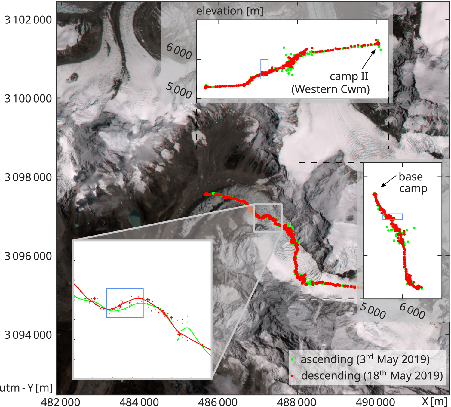
Natural color imagery over Khumbu icefall in the Himalaya range. On the left side is the debris covered Khumbu Glacier, on the right side the top of Mount Everest and Lhotse are almost visible. The GPS points used in this study are overlain on this image. Only the trajectories from Everest base camp to Camp II are shown.
Apart from mapping shear zones for safety issues, information about the flow characteristics in icefalls is useful for a number of glaciological applications. For example, icefalls can be hydrological barriers between the accumulation region and the ablation area, as is suggested both from boreholes (Harper and Humphrey, Reference Harper and Humphrey1995) and velocity evolution (Durkin and others, Reference Durkin, Bartholomaus, Willis and Pritchard2017; Armstrong and others, Reference Armstrong, Anderson and Fahnestock2017). Also, percolation of water and advection of air into the glacier and to the bedrock is more easy though the intense fracturing at the surface (Jarvis and Clarke, Reference Jarvis and Clarke1974; Kodama and Mae, Reference Kodama and Mae1976), making icefalls zones of potentially increased interaction with atmospheric conditions and their changes (Gilbert and others, Reference Gilbert2020).
Glacier behavior at icefalls is characterized by fast-changing and chaotic ice flow velocity. These are particularly difficult to measure under associated conditions. In situ measurements are almost impossible, except from (automatic) time-lapse cameras (Messerli and Grinsted, Reference Messerli and Grinsted2015; Giordan and others, Reference Giordan2016). Measurements based on repeat satellite imagery, which are well established for other zones of glaciers (Heid and Kääb, Reference Heid and Kääb2012; Dehecq and others, Reference Dehecq, Gourmelen and Trouvé2015), tend to fail over icefalls as the ice is flowing too fast, trackable surface patterns are changing too much, and the strong lateral velocity gradients deteriorate accurate window-based pattern matching. In this contribution, we use ensemble matching (also known as time-resolved particle image velocimetry), a technique novel to glaciology, and demonstrate the effectiveness of it using high-repeat Sentinel-2 optical satellite data of Khumbu icefall. The purpose of this contribution is a brief demonstration of the method for glaciologic application, rather than a in-depth technical study or detailed investigation of the ice flow in Khumbu icefall.
Ensemble image matching
Displacement estimation from image matching in the spatial domain
The foundation for displacement estimation from repeat remote sensing is pattern matching (Scambos and others, Reference Scambos, Dutkiewicz, Wilson and Bindschadler1992; Kääb and Vollmer, Reference Kääb and Vollmer2000; Strozzi and others, Reference Strozzi, Luckman, Murray, Wegmüller and Werner2002; Debella-Gilo and Kääb, Reference Debella-Gilo and Kääb2011). It is based on finding a similar template from an image in another larger subsection of an image at a different time instance (t q). Often the similarity measure (ρ) is implemented through normalized cross-correlation as,

Here, ρpq denotes a score surface at discrete step sizes (k, l). It is calculated by the similarity of two templates (Ip and Iq) at different time instances (t p and t q). The upper part of the fraction of equation (1) shifts the intensities in the templates by their mean intensity (denoted by the overbar) to transform the signals to zero-centered variations, while the lower part of the fraction normalizes the contrast of the templates (or intensity spread). This results in a similarity score that can range between −1 and +1.
Matching the velocity over an icefall, or other similarly fast changing surfaces, is much more challenging than on a slow and homogenous flowing glacier tongue. Surface features in an icefall can change quickly over time, thus visual distinctive features, which can be tracked over time, are quickly lost. Furthermore, the flow is first converging and then diverging and thus exhibits considerable shear. Consequently, bulk velocity estimation (of homogenous, simple translation) does not (or not well) work, and in order to fulfill this constrain smaller template sizes are needed, which then lowers the signal-to-noise level (Debella-Gilo and Kääb, Reference Debella-Gilo and Kääb2012). Therefore, in this specific case, we apply pattern matching in the time domain (Meinhart and others, Reference Meinhart, Wereley and Santiago2000), known as ensemble matching (Delnoij and others, Reference Delnoij, Westerweel, Deen, Kuipers and van Swaaij1999), see also the schematic in Figure 2. This means the matching is done with much smaller windows than necessary for common single image pair matching, but instead information is gathered from multiple image pairs of a whole collection. Because some of the imagery will have cloud cover, not all image pairs can be used from the stack, and therefore a selection is made and this we call a collection. With ensemble matching, the same or higher signal-to-noise can be achieved, as a similar total number of image samples (pixels) is taken as is done with single image pair matching, i.e. replacing spatial redundancy by temporal redundancy. When the flow does not change over the analyzed collection period, a clear peak will emerge. Laboratory experiments of sparsely illuminated seeds within a fluid or airmass have shown this spatial resolution can be reduced to a single pixel resolution of independent flow estimates, when an image stack size of several hundreds or thousands of images is included (Westerweel and others, Reference Westerweel, Geelhoed and Lindken2004). For a highly fractured crevasse field, a smaller sample might suffice.
Schematic illustration of the difference between regular single image pair matching and time averaged ensemble matching. Left: single image pair matching requires the application of large window sizes to achieve smooth and clearly defined correlation maxima. Middle: The application of small window sizes and single image pair matching leads to noisy correlation surfaces with small signal-to-noise ratios. Right: Within ensemble matching, the individual noisy correlation surfaces are combined (here: summed) over time to achieve clear correlation peak with high signal-to-noise ratio despite small window sizes.

Sub-pixel localization
Several methods exist to estimate the localization of the correlation peak, which is inherently at pixel level, at sub-pixel resolution. A main difference between the method's implementation is the amount of information needed from the correlation scores surrounding the maximum. Either the directly neighboring pixels are used that are next to the highest score, independently estimating the peak along each axis. A second feature to consider is the shape of the peak, which can be modeled by a parabolic (Argyriou and Vlachos, Reference Argyriou and Vlachos2005), Gaussian (Willert and Gharib, Reference Willert and Gharib1991) or triangular (Olson and Coombs, Reference Olson and Coombs1991) function. Other approaches use all pixels surrounding the highest correlation score, which is the case for center-of-mass, a 2D Gaussian (Nobach and Honkanen, Reference Nobach and Honkanen2005), or a spline (Fahnestock and others, Reference Fahnestock2016) function. The former methods are most popular due to their low computational power, while more computationally expensive methods like upsampling of the imagery and/or its correlation surface is also possible and can achieve precisions in the order of 1/20 of a pixel (Debella-Gilo and Kääb, Reference Debella-Gilo and Kääb2011). In this study, we investigate all the above mentioned methods against upsampling, as systematic errors are present in the different localization methods. It is therefore of importance to assess these different methods for their preferences to integer value displacements, known as peak-locking (or pixel-locking).
Data
Sentinel-2 high repeat satellite imagery
The EU/ESA Copernicus Sentinel-2 mission consists of a constellation of two medium resolution satellites recording visible to shortwave infrared imagery with a spatial resolution down to 10 meter. The first satellite of this mission, Sentinel-2A, was launched in June 2015 and has a same-orbit repeat cycle of 10 days. With the launch of Sentinel-2B in March 2017 into the same orbital plane, this revisit decreased to 5 days from the same orbit. The high dynamic range (12 bit raw) of the Sentinel-2 images makes them ideal for glacier velocity extraction as also areas with little surface contrast show often patterns useful for offset tracking. For correct displacement estimates, imagery from the same orbital track needs to be used (Kääb and others, Reference Kääb2016), as orthorectification errors due to erroneous or outdated elevation models distort the images. Methods are available to correct for these artifacts and make the use of imagery from alongside orbits possible (Altena and Kääb, Reference Altena and Kääb2017). However, in this study, such methods are not the focus and not needed, as the consistent same-orbit monitoring by Sentinel-2 provides enough imagery suited to demonstrate the method and derive a useful velocity field over the Khumbu icefall.
Location-aware sport wearables
For independent comparison to our velocity data, we use trajectory data collected by high-altitude mountaineers. These climbers move through the Khumbu icefall while equipped with location-aware wearables. These handheld GPSs have sensors that are able to record position, altitude and heading during outdoor activity. Afterwards the data can be uploaded to online sports diaries, where these can be shared either within the respective communities or archived into a private collection. Accumulation of such spatio-temporal datasets can be used to extract geographic information, mostly done through trajectory clustering, patterns or prediction (Giannotti and Pedreschi, Reference Giannotti and Pedreschi2008).
These types of positioning data can be used in different ways, depending on spatial and temporal selection criteria. Definitions are therefore given about such groupings for this data-type. For instance, a ‘trajectory’ is a collection of positioning points connected to each other by an increasing and ordered timestamp. A ‘trail’ is a collection of positioning points on a line without a time instance. If several trajectories are close together in space and time they are called a ‘flock’. Then, when a flock is in close proximity to a trail, they are called a ‘convoy’.
During a climbing ascent through the icefall, the data collection is thus as a convoy. However, in our case, the multi-temporal sequences can be seen as being within an environment that changes over time (Wiratma and others, Reference Wiratma, van Kreveld and Löffler2017). In our situation, we assume the flock follows a trail, but the trail has a temporal character; as the glacier moves with the trail on top. Consequently, glacier velocity can be extracted over time from different flocks.
Implementation
The general workflow of our implementation is illustrated in Figure 3. The image collection is used to generate a general scene. This general appearance of the icefall is used to identify correct imagery without much cloud cover. If selected images have the correct time separation between each other, they are matched and used to build the ensemble correlation surface. The details of these steps are discussed in the sections hereafter.
Schematic illustration of the general workflow adopted in this study.

Cloud-free scene classification
Cloud cover hampers the ability to extract within-season imagery for many optical Earth observation systems like Landsat (Ju and Roy, Reference Ju and Roy2008). The optical instruments of Sentinel-2 are also hampered by the cloud coverage, but this constellation has an increased revisit rate of 5 days, increasing the possibility to get many pairs of images with a short acquisition interval even if a number of scenes are affected by cloud cover. Due to the resulting large data volumes, the collection of useful imagery requires automatic classification of cloud cover. Global cloud cover products in the Sentinel-2 meta-data can be used, but these would exclude partly clouded or highly clouded scenes, even if the very location of interest (here the icefall) is actually cloudfree. The detection of clouds in high mountain terrain is challenging due to snow cover and topographic shadowing. Therefore, we use all the images and stack statistics (median) at the pixel level to generate a scene composite (or stack-median, $\tilde {{\bf I}}$ ) (Winsvold and others, Reference Winsvold, Kääb and Nuth2016). The stack-median is then converted by a 2D Fourier transform, and its absolute values are taken and transformed by their natural logarithm ($\ln {\Vert {\cal F}\lpar \tilde {{\bf I}}\rpar \Vert }$
 ). These operations result in a distinct pattern description, particularly present in natural images (Torralba and Oliva, Reference Torralba and Oliva2003), and gives a mean to compare against other transformed images. Thus, every image is transformed by these operations, and the resulting image description is matched against the stack-median. The similarity metric calculated for this comparison is mutual information (Viola and Wells III, Reference Viola and Wells III1997). These mutual information scores are ultimately used to classify imagery into cloud-free and cloud-covered. This class separation is achieved through a two-class k-means procedure, resulting in an binary cloud-cover attribute to each image that is used to build the collection of images suitable for ensemble matching.
Icefall displacement from Sentinel-2
Currently, the absolute localization of Sentinel-2 is done through its sensor readings, hence its variability is in the order of 10 meter (Gascon and others, Reference Gascon2017). Each image is therefore in our study co-registered by simple translation to the stack-median, using conventional image matching over stable terrain (Leprince and others, Reference Leprince, Barbot, Ayoub and Avouac2007), and each individual image is interpolated towards this base image. The stack-median is thus also affected by the same co-registration noise. However, these varying offsets do not seem to cause much blurring in the stack-median. This might however be the case for image collections with worse registration accuracy than Sentinel-2, or when significantly less images are stacked.
The individual images are then ordered into pairs from the same relative orbital track (in this case R076) and matched if they are separated by 10 days. This time-span seems to be a good compromise between significant spatial movement in relation to degradation of traceable appearance as ice flows through the icefall, where it melts and fractures. Hence, imagery of the same Sentinel-2 orbit and satellite is matched with each other. In this way also data from January 2016 onwards can be used, the time when only Sentinel-2A was in orbit. The last acquisitions used in this study are from October 2019. Given the time-span constrain of 10 days, a total of 53 pairs are matched against each other, with a template (Ip) size of three pixels, while the search space is five pixels wide.
Icefall displacement from GPS trajectories
The mountain climber trajectories of an ascending (3rd of May) and a descending track (18th of May) were used for comparison to our surface velocity estimate. The tracks come from a Norwegian climbing team that used Garmin inReach satellite positioning devices as they climbed through Khumbu icefall in 2019, toward Camp II and Mount Everest. One of the devices has been set to record every minute, while another member recorded at a 10 min interval (· and + in Fig. 1, respectively). For a large extent, the path goes straight against the flow direction of the glacier. In addition, the positioning data are very noisy, most presumably due to multi-path signals from the surrounding peaks and steep ice walls (i.e. the large spread in elevation in the subplots of Fig. 1). There is only a small part of the route where the trail is perpendicular to the flow, and it is this region, which is here used as validation against the ensemble matching estimate. The trajectories were first pre-processed through a Hampel filter (Lee and Krumm, Reference Lee and Krumm2011) and then a cubic smoothing spline was interpolated through these points. A smoothing parameter of 5 · 10−5 was chosen and checked for consistency with the 10 min-interval dataset. At the velocity sampling distance of 30 m, the closeness (Wiratma and others, Reference Wiratma, van Kreveld and Löffler2017) of the ascending trajectory to the descending trajectory in the direction of glacier flow was then measured to extract a glacier velocity estimate.
Results and discussion
The automatic cloud detection through a stack-median and spectral matching through mutual information gives a success rate of roughly 80%. While more advanced methods might work, this score is reasonable for this application, as cloud scenes might only lower the signal-to-noise, but will not introduce a velocity bias. We think the high success rate of the classification is mainly due to the large volume of Sentinel-2 imagery available in the archive that seems sufficient to generate a good composite of the general appearance of the scence by the stack-median. Further success is due to the frequency distribution of clouds; their signature in the power spectrum seems to be sufficiently different from topography. A seasonal dependency is present in our classification, as many scenes within the summer season are assigned as cloudy imagery. As the selected scenes fall outside of the monsoon season, the extracted velocities from the ensemble matching will mostly represent the winter velocities on Khumbu Glacier.
Icefall velocity field
The absolute surface velocity estimation over Khumbu icefall is illustrated in Figure 4. Where the maximum velocity seems to be just over 1 m d−1. Two distinct patches of fast flow occur after each other, aligning with the steepest sections of the icefall. It seems these faster velocities are situated just upstream of an increase in slope (see inset of Fig. 4). These spatial patterns of velocity differences show the achievable detail of this method. Though we should note that the velocity shown here are planimetric velocity and these estimates are not corrected or normalized with the slope of the terrain.
Hillshading drapped with colorcoded surface velocities from ensemble matching over the Khumbu icefall, given in meter per day (m d−1). The template used is 30 m wide, sub-pixel localization is done with 2D-spline interpolation, and peak-locking correction was applied through a secondary off-setted displacement estimation. The results from this ensemble matching can be compared to the results from standard single-pair matching in Figure 5. The inset on the left shows colorcoded slope estimates from a very high-resolution spaceborne digital elevation model (DEM) from Shean (Reference Shean2017) along a flowline, as indicated by the black arrow. Overlayed are the same ensemble velocity estimates as the image, but this time as contours.

Figure 5 shows three examples of pair-wise template matching for May 2018 with Sentinel-2 data. The upperleft frame in Figure 5 shows an estimate of the annual velocity from ITSLIVE for 2018, generated using auto-RIFT (Gardner and others, Reference Gardner2018). This estimate is based on Landsat 8 imagery, has a sampling interval of 240 m, and uses median statistics over a large collection of velocity fields. These annual estimates clearly show that a long separation time up to hundreds of days complicates the generation of sufficient results over the icefall, though the slower moving ice at the tongue is captured. The other insets are velocity estimates stemming from two Sentinel-2B scenes (on 8 and 18 May 2018), which is in the same time period as the GPS trajectories, as shown in Figure 1. The different solutions shown in Figure 5 are due to the use of different template sizes, but the sampling distance is every 30 m. Foremostly, the smoothing and thus dampening of the signal is apparent, as the template size increases. The amount of spatial detail present in the 30 m solution is comparable to the ensemble matching, it is though significantly more affected by noise. There was no filtering applied to the ensemble solution (Fig. 4), and there seems no filtering necessary which is a great benefit. The velocities in early May 2018 seem to be faster than the ensemble solution, which uses pairs mostly outside of the spring and summer season.
(a) Annual glacier velocity estimate of 2018 over Khumbu Glacier from ITSLIVE. These velocity estimates are low and are given a different colorcoding than in the other panels. The background is a Sentinel-2B scene on 8 May 2018, which is one of the images used for velocity extraction of the other velocity estimates in this figure. (b–d) ‘Classical’ velocity estimate from a pair of Sentinel-2 images with 10 day interval, but different sizes of template windows used.

Sub-pixel localization
In order to assess the different sub-pixel localization approaches, we up-sampled all imagery by a factor of ten, to get an estimate to be used as reference. The statistics of their comparison against this dataset is listed in Table 1 Both classical and robust statistical measures are shown, as especially the triangular method has many outliers within. Representing the correlation peak through a triangular shape assumes an ideal measurement system, where simple translation resolves in an ideal pulse in the correlation surface. However, due to flow variation of the ice and change in appearance of the terrain, smoothing of the top of the correlation peak occurs. Neighboring correlation scores can therefore be relatively high, deviating from the pointy model of a triangle and causing location estimates far larger than half a pixel. Thus, from here onwards the triangular localization is neglected from our analysis.
Group statistics of on-glacier sub-pixel localization, against up-sampled imagery

The smallest entity for each measure is highlighted.
The statistics in Table 1 give a general overview of the localization performance, but also an optimistic view of precision. Since large portions of the glacier are flowing slowly, these regions are overrepresented in these statistics. In general, this might not be an issue, but pixel-localization methods suffer from ‘peak-locking’, where a preference exist toward integer values (Willert and Gharib, Reference Willert and Gharib1991; Westerweel, Reference Westerweel1997) causing a bias. This bias stems from large variations of correlation values around the correlation peak, hence the localization methods will prefer to stay close to integer value. This large variation in correlation scores is especially the case for ensemble matching, where correlation surfaces with low signal-to-noise ratios are summed-up.
The reference dataset used for this assessment is without sub-pixel localization, and has thus a resolution of 0.1 pixel. Hence, grouping the statistics into these increments gives an improved insight into the peak-locking bias present in the estimates, as it gives the opportunity to distangle the group statistics into sub-distributions. Such distributions are shown in Figures 6a and b for on-glacier velocity estimates which have a displacement of one-tenth of a pixel in the reference dataset. Here the differences between the reference dataset and the different peak localization methods are shown. If no-bias would exist then the mode and mean would be centered around zero. However, there is a significant skew present, especially for the parabolic and spline localization. Furthermore, a secondary peak is present at a tenth of a pixel distance (in line with the vertical lightgray axis). This peak is caused because the localization method was not able to estimate within bounds of the peak, being further than half a pixel. The tendency in both sub-distributions is toward this secondary peak, showing the sensitivity for peak-locking. From these statistics, the Gaussian methods seem to have less dependency on peak-locking (Westerweel, Reference Westerweel1997). However, for the one-dimensional Gaussian estimator, a significant amount of peak locations could not be estimated. This can stem from the natural logarithm function within the Gaussian estimator that transforms white noise asymmetrically (Anthony and Granick, Reference Anthony and Granick2009).
Histograms of shift differences between several subpixel estimators and the reference dataset are shown in (a) and (b), the reference dataset was upsampled by a factor of ten. The distributions are a selection of all the pixels, these are all estimates that shifted by 1/10 of a pixel according to the reference dataset. (a) Distribution of − 0.1 pixel displacement, (b) distribution of + 0.1 pixel displacement.

Compensation for peak-locking can be done by re-interpolation, looking at the group statistics and smooth accordingly (Christensen, Reference Christensen2004). However, the distribution of velocities needs to stretch over multiple integer values, which is not the case here. Another option is to systematically offset one of the images by half a pixel (Shimizu and Okutomi, Reference Shimizu and Okutomi2002). The introduced offset is also affected by peak-locking, but its dependency is in the other direction and can thus compensate for the peak-locking bias. This method is applied here, and the two results for spline interpolation are shown in the Figure 7. Variation on stable terrain is considerably more in the offset version in respect to the original. When combined, an estimate with less bias can be calculated, as shown in Figure 4. A similar analysis as is done previously with the standard estimation can be done with the adjusted estimates, as is shown in Figures 8a and b. Here a clear difference seems to emerge between the parabolic and the spline estimators. The parabolic estimate still has large peak-locking effects, while the spline method seems to align most centered to zero, with less skew than the others. While the Gaussian methods have a slight peak-locking dependency and more variability. The one-dimensional Gaussian method has a considerable amount of location estimates outside of the sub-pixel range (Fig. 6), and for these estimates, it is not possible to be compensated. Hence, here as well, the two-dimensional method is preferred over the one-dimensional.
Split window between velocity estimates for ensemble matching with original co-registered imagery, and ensemble matching with a systematic offset of half a pixel, which is later removed. Both sub-pixel localization estimates use the spline interpolation. The mean velocity of these estimates are shown in Figure 4.

Histograms of shift differences between several subpixel estimators with a compensation by a systematic offset of half a pixel and the reference dataset are shown in (a) and (b), the reference dataset was upsampled by a factor of ten. Here, the distribution is shown for all pixels which are shifted by 1/10 of a pixel according to the reference dataset. (a) Distribution of − 1/10 pixel displacement, (b) distribution of +1/10 pixel displacement.

GPS trajectories through the icefall
There is a general and consistent underestimation of the ensemble matching estimates in relation to the in situ measurements (Fig. 9a). This can be due to (i); the noisy nature of satellite positioning; or (ii) the measurement interval of both measurements (Fig. 9b), as the GPS velocities are in spring and might not be in line with annual velocities. Thus, the short time interval of the GPS velocities might capture higher spring velocities that stem from a larger sliding component underneath the icefall than the average during the entire melting period. This is supported by the individual matching estimates in summer, as shown in Figure 5, which give also higher estimates than the ensemble estimate. This is also observable in Figure 9a, where individual velocity estimates (×) are consistently larger than the ensemble estimate ($\bullet$ ).
).
(a) Comparison of the different subpixel estimates to the GPS displacements, indicated by circles ($\bullet$ ). The crosses (×) stem from a single pair of Sentinel-2 images in spring, this velocity field is also shown in Figure 5c. (b) Shows the image time serie of Sentinel-2 and the associated cloud-free classification. The monsoon seems to create a gap in the summer months. (a) GPS comparison to ensemble, (b) Sentinel-2 scene selection over time

Conclusions and perspective
To the best of our knowledge, our study is the first to test ensemble matching outside of controlled laboratory environments and in a typical remote-sensing setting. Eventhough it is a specialized technique, it has an application domain in combination with the high-repeat imagery of Sentinel-2. Previously, it has not been possible or at least difficult to extract velocity estimates over fast-flowing and fast-changing glacier zones such as icefalls, as demonstrated here over Khumbu icefall (see figures in Scherler and others, Reference Scherler, Leprince and Strecker2008; Rowan and others, Reference Rowan, Egholm, Quincey and Glasser2015; Haritashya and others, Reference Haritashya, Pleasants and Copland2015; Rounce and others, Reference Rounce, King, McCarthy, Shean and Salerno2018). Typically, the velocities on the tongue of a glacier are measured using repeat optical satellite images, as in the case of Khumbu Glacier is downstream from Everest base camp (Bolch and others, Reference Bolch, Buchroithner, Peters, Baessler and Bajracharya2008). The constrain set by large window sizes in classical pattern matching is not limited to optical remote sensing alone, and SAR speckle tracking (Quincey and others, Reference Quincey, Luckman and Benn2009) has not been able to resolve this part of Khumbu Glacier either. However, the ensemble matching technique is transferable to the SAR domain, and we think is able to enhance SAR offset tracking results in a similar fashion as presented here.
Recently, encouraging results have been produced through the use of stacking of displacement fields and using weighting or median filtering, generating products with a resolution at 50 m (Nobakht and others, Reference Nobakht, Motagh, Wetzel, Roessner and Kaufmann2014; Millan and others, Reference Millan2019) with Sentinel-2, or 100/125 m with Landsat 8 (Shen and others, Reference Shen2018; Gardner and others, Reference Gardner2018). However, these results are based on large window sizes followed by spatial smoothing, and the such-generated estimates might thus not align with the true velocity gradients. Such smoothing is not done in this study, and the inherent detail and errors of the icefall surface velocity are clearly observed. Neither did we apply any post-processing in this study, while except from steep mountain ridges, clear outliers do not seem to occur on the icefall in our estimate. This makes the matching more transparent, straight forward and complete than for many previous approaches where method differences lie often more in the post-processing than in the matching itself (Heid and Kääb, Reference Heid and Kääb2012). The amount of imagery used here (53 pairs) might by far be sufficient, which shows the opportunity to use this technique to resolve annual or even seasonal estimates with less pairs. In addition, we identify systematic differences between the different sub-pixel localization methods. From our analysis, we can state that there seems to be a superiority in spline methods. However, compensation for peak-locking is needed. Practically, this means the ensemble matching needs to run a second time. Because the correlation score surface in the spatial domain is used, other sub-pixel localization methods that are based on the frequency domain are not assessed here (i.e.: TPSS Leprince and others, Reference Leprince, Barbot, Ayoub and Avouac2007, sinc-function Rösgen, Reference Rösgen2003). Because of the summation or stacking of correlation surfaces, it is neither possible to assess iterative sub-pixel estimators that work on the imagery directly (i.e. differential methods Lucas and Kanade, Reference Lucas and Kanade1981). These methods might be less affected by peak-locking, thus our results can only for a limited amount be transferred to image pair matching.
Lastly, the limited amount of in situ GPS trajectory data restricts our comparison effort, but we demonstrate this data type as an interesting source to extract information in unconventional ways.
Acknowledgements
We thank Didrik Bakke Dukefoss and Thomas Erling Lone, the high-altitude mountaineers that were willing to share their positioning data of the tracks which they climbed through Khumbu icefall while making a successful ascent to Mount Everest. We also thank two anonymous reviewers for their input, which helped to improve the manuscript, and Rachel Carr for handling the review process as editor. This research and development has been conducted through support from the European Union FP7 ERC project ICEMASS (320816) and through ESA Living Planet Fellowship to B.A., Glaciers-CCI, CCI+ and EE10 HARMONY projects (4000125560/18/I-NS, 4000109873/14/I-NB, 4000127593/19/I/NB, 4000127656/19/NL/FF/gp). The code will be available on http://www.runmycode.org/coder/view/3479.
Supplementary material
To view supplementary material for this article, please visit https://doi.org/10.1017/jog.2020.66
Appendix
Sub-pixel estimates of both the North-South (Fig. 10) and East-West (Fig. 11) direction here in the Appendix. The corresponding statistics and distribution plots are shown in Table 1, Figure 6 and the main text.
Sub-pixel localization for the Y-component (North-South) of Khumbu icefall, where the color scale goes from red for −0.5, white is 0 and blue is +0.5, in pixel spacing. (a) 1D Parabolic; (b) 2D spline; (c) 1D Gaussian; (d) 2D Gaussian; (e) 1D triangular (f) 2D center of mass; (g) upsampled; (h) integer displacement

Sub-pixel localization for the X-component (East-West) of Khumbu icefall, where the color scale goes from red for +0.5, white is 0 and blue is −0.5, in pixel spacing. (a) 1D Parabolic, (b) 2D spline, (c) 1D Gaussian, (d) 2D Gaussian, (e) 1D triangular, (f) 2D center of mass, (g) upsampled, (h) integer displacement.


 Open access