


1. Introduction
Liquid water exists beneath glaciers and large ice masses in a variety of different environments from small alpine glaciers to large polar ice sheets (Bell, Reference Bell2008; Siegert and others, Reference Siegert2018). Subglacial water can be dynamic and flows through drainage networks contributing to fast-flowing glacier and ice-stream processes (Blankenship and others, Reference Blankenship, Bentley, Rooney and Alley1987; Engelhardt and Kamb, Reference Engelhardt and Kamb1997; Le Brocq and others, Reference Le Brocq2013). On the other hand, basal water can be static and reside in isolated water bodies located in bedrock depressions of slow-moving ice potentially for up to many thousands of years (Dowdeswell and Siegert, Reference Dowdeswell and Siegert1999; Siegert and others, Reference Siegert, Taylor and Payne2005b; Wright and Siegert, Reference Wright and Siegert2012). Water can also be stored in the pores of sediments within subglacial aquifer systems (e.g. Lingle and Brown, Reference Lingle, Brown, Van der Veen and Oerlemans1987; Siegert and others, Reference Siegert2018), or in active subglacial lakes which can fill and drain on annual to decadal time scales (Siegert and others, Reference Siegert, Carter, Tabacco, Popov and Blankenship2005a; Fricker and others, Reference Fricker, Scambos, Bindschadler and Padman2007; Wright and Siegert, Reference Wright and Siegert2012; Bowling and others, Reference Bowling, Livingstone, Sole and Chu2019). The presence, movement, volume and properties of water beneath glaciers not only affect the dynamics of the overlying ice (key for predicting the evolution of glaciers and ice masses, Christoffersen and others, Reference Christoffersen, Bougamont, Carter, Fricker and Tulaczyk2014; Siegert and others, Reference Siegert2018), but also have important implications for potential subglacial habitats, where microbial life has been found in the presence of liquid water, despite extreme cold (and saline) conditions (Mikucki and others, Reference Mikucki, Foreman, Sattler, Lyons and Priscu2004, Reference Mikucki2009; Michaud and others, Reference Michaud2016).
Subglacial water can originate from surface water draining to the bed through moulins, crevasses and fractures (Zwally and others, Reference Zwally2002); melting of the ice-sheet base from geothermal heating (Blankenship and others, Reference Blankenship1993) and basal friction (Bell, Reference Bell2008); or influx from underlying aquifers (Christoffersen and others, Reference Christoffersen, Bougamont, Carter, Fricker and Tulaczyk2014). This water flows over or through bedrock and sediment, which can provide reaction sites for chemical and biological weathering, with the drainage configuration determining the length of time for water–rock interactions and solute generation. These chemical and biological processes can generate aqueous microbial ecosystems, which feed off dissolved solutes (Tranter and others, Reference Tranter2004). Direct sampling of an Antarctic subglacial lake beneath 800 m of ice on the Whillans Ice Stream, West Antarctica, confirmed the presence of a viable microbial ecosystem surviving in this extreme environment (Christner and others, Reference Christner2014; Achberger and others, Reference Achberger2016). These terrestrial subglacial water systems can therefore be considered as potential analogs for microbial habitats on extraterrestrial frozen planetary bodies, where liquid water has been inferred beneath the ice (Carr and others, Reference Carr1998; Lauro and others, Reference Lauro2020).
Brine-rich water depresses the freezing point and can exist at temperatures well below 0°C. For example, Hubbard and others (Reference Hubbard, Lawson, Anderson, Hubbard and Blatter2004) showed evidence for brine-rich water with a temperature of −7.8°C beneath the Taylor Glacier in the McMurdo Dry Valleys, Antarctica, using ground-penetrating radar (GPR). At Taylor Glacier, the brine is thought to have originated from seawater intrusion during the Miocene where subsequent climatic cooling may have led to a build-up of salts through freezing of the saline water. For example, when the saline water froze over time, the denser salt was expelled during the freezing process and increased the salinity of the remaining unfrozen water, also known as cryoconcentration (Elston and Bressler, Reference Elston and Bressler1981; Sugden and others, Reference Sugden, Denton and Marchant1995). Recently, Rutishauser and others (Reference Rutishauser2018) detected a potential hypersaline subglacial lake complex under the Devon Ice Cap in the Canadian Arctic under 800 m of ice, in a region previously inferred to be cold-based, where the ice is frozen to the bed. Modeled basal ice temperatures suggest a lake complex temperature of ~−14.5°C, with the solute for the brine coming from an underlying evaporate-rich sediment unit containing interbedded salt sequences. The presence of liquid water in cold-ice regions has implications for basal sliding contributions to ice dynamics, which have, to date, been discounted in such locations. Furthermore, because of the cold and hypersaline nature, the Devon subglacial lake complex may represent one of the closest terrestrial analogs for brine bodies inferred to exist on Europa (Schmidt and others, Reference Schmidt, Blankenship, Patterson and Schenk2011), Enceladus (Postberg and others, Reference Postberg, Schmidt, Hillier, Kempf and Srama2011) and Mars (Lauro and others, Reference Lauro2020).
Typical geophysical techniques used for detailed investigation and mapping of subglacial water include airborne radar (e.g. Schroeder and others, Reference Schroeder, Blankenship, Raney and Grima2014; Rutishauser and others, Reference Rutishauser2018), GPR (e.g. Hubbard and others, Reference Hubbard, Lawson, Anderson, Hubbard and Blatter2004; Kulessa and others, Reference Kulessa, Booth, Hobbs and Hubbard2008; Christianson and others, Reference Christianson, Jacobel, Horgan, Anandakrishnan and Alley2012) and active source seismic (e.g. Peters and others, Reference Peters2008; Horgan and others, Reference Horgan2012; Dow and others, Reference Dow2013). Radar methods are well suited to characterizing the internal structure of the ice column, the basal topography and lateral extent of subglacial water systems. However, in the case of a subglacial lake, high reflectivity of the ice–water interface and high attenuation within the lake limit the utility of radar sounding to sample beneath the ice–water interface. Active source seismic reflection methods can be used to image stratigraphic horizons such as subglacial lake–bedrock boundaries and, by applying amplitude-versus-offset and anisotropy techniques, they also provide estimates of the mechanical properties of ice and subglacial material (e.g. Anandakrishnan, Reference Anandakrishnan2003; Booth and others, Reference Booth2012; Dow and others, Reference Dow2013; Diez and others, Reference Diez and Eisen2015; Kulessa and others, Reference Kulessa2017). However, seismic methods often lack the resolution and signal-to-noise ratio to quantify subglacial material properties beyond the immediate ice–bed interface. Furthermore, both radar and seismic techniques cannot directly derive the salinity of the water, which is important for determining the temperature and freezing point of these subglacial liquid water environments, and the role that the presence of salt-bearing rock can play in their persistence.
Therefore, geophysical techniques more sensitive to fluid-content contrasts, such as electromagnetic (EM) methods, are required to fully characterize subglacial water systems (Key and Siegfried, Reference Key and Siegfried2017). Transient electromagnetic (TEM) methods offer a promising means of characterizing and quantifying subglacial water by inferring the resistivity structure of the subsurface. This technique is particularly applicable for glaciological studies due to the large difference in electrical resistivity between ice and liquid water, because electrical resistivity increases by several orders of magnitude when water freezes (McNeill and Hoekstra, Reference McNeill and Hoekstra1973). Furthermore, the resistivity of water strongly decreases with salinity (Perkin and Lewis, Reference Perkin and Lewis1980). TEM methods have been used extensively for mapping groundwater hydrology in non-glaciated environments (e.g. Fitterman and Stewart, Reference Fitterman and Stewart1986; Auken and others, Reference Auken, Jørgensen and Sørensen2003; Danielsen and others, Reference Danielsen, Auken, Jørgensen, Søndergaard and Sørensen2003; Auken and others, Reference Auken, Christiansen, Jacobsen and Sørensen2008; Delsman and others, Reference Delsman2018) and permafrost thickness in polar and mountainous regions (e.g. McNeill and Hoekstra, Reference McNeill and Hoekstra1973; Hauck and others, Reference Hauck, Guglielmin, Isaksen and Vonder Mühll2001; Foley and others, Reference Foley2020). However, to date, very few TEM surveys have been acquired in glaciated environments to map subglacial water and its salinity. The success of Mikucki and others’ (Reference Mikucki2015) airborne TEM survey in the East Antarctic dry valleys, which showed an extensive deep saline groundwater system, has motivated feasibility studies and concept papers discussing and highlighting the potential of EM methods for imaging subglacial hydrology (e.g. Key and Siegfried, Reference Key and Siegfried2017; Siegert and others, Reference Siegert2018; Hill, Reference Hill2020).
In this study, we continue the development of EM methods for quantifying subglacial water characteristics, specifically focusing on the TEM technique, using synthetic modeling. We present a novel methodology for deriving the salinity of subglacial water, along with quantitative uncertainty analysis. We use a variety of one-dimensional (1-D) and quasi two-dimensional (2-D) synthetic models to illustrate how TEM methods can be used for imaging in an ice-sheet environment, highlighting the method's strengths and limitations for characterizing and quantifying subglacial water systems.
2. Method
2.1. Transient electromagnetics
Both airborne and ground-based EM methods (Fig. 1a) have been used globally, in non-glaciated environments, to search for groundwater (Auken and others, Reference Auken, Jørgensen and Sørensen2003) and map the extent saltwater and/or contaminant intrusions (Buselli and others, Reference Buselli, Barber and Zerilli1988; Pedersen and others, Reference Pedersen2017), by exploiting the difference in electrical resistivity between pore fluids and the adjacent sediments/bedrock. In a glaciated environment, ice has an extremely high electrical resistivity (104–105 Ωm; Petrenko and Whitworth, Reference Petrenko and Whitworth2002; Kulessa, Reference Kulessa2007) compared to groundwater (10−1–102 Ωm; Roberge, Reference Roberge2006). Furthermore, fresh groundwater, 1–102 Ωm (20–0.1 practical salinity units (psu)), has a higher electrical resistivity than saline water, 10−1–1 Ωm (200–20 psu) (Perkin and Lewis, Reference Perkin and Lewis1980). This is due to the concentration and mobility of ions, where low-impurity ice causes the slow movement of sparse ions (providing a high resistance) and liquid water enables the ions to move freely. Although pure deionized fresh water has a resistivity of 104 Ωm (Roberge, Reference Roberge2006), the addition of a small number of ions, in the form of dissolved solutes to liquid water greatly decreases the electrical resistivity. In a subglacial setting, the resistivity can be used as a measure of groundwater residence time, where newly formed basal meltwater from clean ice will have a low ion concentration, hence high electrical resistivity. In contrast, older mixed waters with longer water–rock interactions have increased ionic content from geochemical dissolution of adjacent sediments/bedrock and hence have low electrical resistivity (Key and Siegfried, Reference Key and Siegfried2017).
(a) Schematic diagram of TEM methods acquired on ice masses, highlighting the different techniques used for different thicknesses of ice. (b) Schematic diagram of the transmitter waveform for a small (pink) and large (blue) ground-based TEM system, where the current in the transmitter loop flows in the opposite direction in the second half of the transmitter cycle. (c) Maximum depth of investigation for small (pink) and large (purple) ground-based TEM systems and airborne systems (black) (Mikucki and others, Reference Mikucki2015). For the ground-based systems, we plot the approximate DOI for the Geonics TEM-47 (small) system (Geonics, 1994) and the Geonics TEM-67 (large) system (Geonics, 2012), calculated using Eqns (S1) and (S2), respectively, which are approximated versions of Eqn (2).

TEM methods determine the electrical resistivity of the subsurface by using a transmitter loop with a time-varying primary current to induce secondary electric currents in the subsurface (Fig. 1b). The transmitter current is often a square wave with period T. From time t = 0–T/4 the current is on, from t = T/4–T/2 the current is turned off, from t = T/2–3T/4 the current is on but with reversed polarity and from t = 3T/4–T the current is off. Each time the primary current is turned off, secondary currents are induced in the Earth. These secondary (eddy) currents produce a secondary magnetic field, which can be measured at the receiver on the surface (Fig. 1a). The secondary electric currents decay with time and this decay can be monitored through the secondary magnetic field that they generate. Depth sounding is made possible by two principles. Firstly, the secondary currents decay quickly in resistive material and more slowly in conductive material. Thus, observations of the decay rate provide information about the subsurface resistivity. Secondly, the secondary current system moves to greater depths over time. In a halfspace, the depth of investigation (DOI) at a time (t) is given by (δ T)

where the resistivity (ρ) and magnetic permeability (μ 0 = 4π × 10−7 N/A2) define the Earth structure. Note that in the absence of any magnetic materials in the typical glacial environment, the free space value of magnetic permeability was used. The receiver measures the induced secondary magnetic field during the time when the transmitter is switched off. This measurement is made from the voltage induced in the receiver by the time variation of the decaying secondary magnetic field. The receiver voltage is recorded as a function of time, where later responses originate from greater depths. A non-linear inversion process is then used to infer the variation of resistivity with depth from the data (receiver voltages as a function of time (e.g. Barnett, Reference Barnett1984; Constable and others, Reference Constable, Parker and Constable1987; Christensen and Tølbøll, Reference Christensen and Tølbøll2009; Vignoli and others, Reference Vignoli, Fiandaca, Christiansen, Kirkegaard and Auken2014; Auken and others, Reference Auken2015)).
The maximum DOI (h) of a TEM system is dependent on the area of the transmitter coil (A), transmitter current (I), background noise level (ηV) and underlying resistivity (ρ) of the subsurface (Spies, Reference Spies1989).

Equation (2) is the late-time approximation, and uses the fact that data are recorded as long as the transient is greater than the background noise level. Deeper sounding can be achieved with a stronger signal and/or lower noise levels. Small ground-based systems generally use transmitter loop sizes ranging from 5 × 5 m to 100 × 100 m with transmitter currents ~1–3 A. These small systems are commonly used for characterizing the near subsurface and are quick and efficient to deploy in a glaciated environment. Killingbeck and others (Reference Killingbeck, Booth, Livermore, Bates and West2020) demonstrated that a 10 × 10 m transmitter coil with 2 A could image down to 90 m DOI, which included 25 m of ice and 65 m of conductive wet subglacial sediments. Airborne TEM systems use a ~500 m2 transmitter loop with four wire turns and a maximum current of 95 A towed by a helicopter ~35 m above the ground. With airborne TEM surveys in the dry valleys in East Antarctica, Mikucki and others (Reference Mikucki2015) found the maximum DOI over low-resistivity surface lakes was ~100 m, and over high resistivity permafrost/ice was 350 m. Airborne TEM is by far the most efficient method for spatial coverage and surveying inaccessible areas, for example, imaging under highly crevassed glaciers. However, this application is not suitable for ice masses thicker than ~350 m, and is unable to map groundwater stored in porous sediments or bedrock >350 m depth. This is because the signal from these deep water bodies would most likely be below the airborne system's noise level (Key and Siegfried, Reference Key and Siegfried2017). Large ground-based systems generally use transmitter loop sizes ranging from 100 × 100 m to 1000 × 1000 m with transmitter currents ~10–28 A and can potentially image under ice up to 1000 m thick (Fig. 1c). Ground-based systems generally use smaller currents than the airborne system, but with much larger, single turn, transmitter loop areas, resulting in different DOIs for each system. Although large loop sizes can be less efficient to deploy than small loops and airborne systems, they can be deployed relatively easily in glaciated environments with the use of snow mobiles. Furthermore, over glaciers and ice sheets, there are fewer obstacles to negotiate compared to non-glaciated and urban settings, where buildings, power lines, vegetation and topographic variations can complicate the deployment of large loops. Most importantly, ground-based large loop systems can collect data with a much higher signal-to-noise ratio than airborne systems, due to their significantly larger transmitter dipole moment and longer stacking times, making it possible to image deeper into a subglacial hydrological environment (Key and Siegfried, Reference Key and Siegfried2017).
2.2. TEM inversion for resistivity
Like most geophysical inversions, the inversion of TEM data is non-unique, i.e. many resistivity-depth profiles will fit the observed TEM data to within the statistical errors of the data. Non-uniqueness can arise from both (1) poor quality data and (2) the inherent physics.
The second type of non-uniqueness is the most challenging and can only be addressed with a complete understanding of the underlying physics. For example, if the model contains a conductive layer, the TEM data are primarily sensitive to the conductance (the product of conductivity and thickness) rather than layer conductivity or thickness alone. Therefore, a thin conductive layer (e.g. a 5 m-thick saline subglacial lake with resistivity 1 Ωm) could produce a similar TEM response to a thick, less conductive layer (e.g. 50 m-thick saturated subglacial sediment at 10 Ωm). Thus, to determine the thickness and conductivity of a subglacial water body separately, the TEM method cannot be used on its own. External information such as borehole, seismic or radar data is required to overcome this non-uniqueness (Christensen and Tølbøll, Reference Christensen and Tølbøll2009; Vignoli and others, Reference Vignoli, Fiandaca, Christiansen, Kirkegaard and Auken2014; Auken and others, Reference Auken2015).
In geophysical inversions, prior information from multiple independent datasets can constrain the model space, by combining their depth and resolution sensitivities. Glaciological surveys often involve the acquisition of multiple datasets, for example, seismic, radar and boreholes, as imaging the target with several methods can provide a more robust interpretation (e.g. Merz and others, Reference Merz2016). Recently, Killingbeck and others (Reference Killingbeck, Booth, Livermore, Bates and West2020) developed a probabilistic inversion methodology called MuLTI-TEM to combine these datasets numerically. In this study, we further develop this algorithm into a new version called MuLTI-TEMP, which quantitatively derives the salinity of subsurface fluids using additional petrophysical analysis, discussed further in Section 2.3. Here, we describe the methodology and outputs of the original MuLTI-TEM algorithm, although for a more detailed description, see Killingbeck and others, Reference Killingbeck, Booth, Livermore, Bates and West2020.
MuLTI-TEM is a Bayesian inversion written in MATLAB that uses independent depth constraints (e.g. borehole, radar or seismic lithological boundaries) to provide statistical properties and uncertainty analysis of the resistivity profile with depth. The method uses a trans-dimensional Markov Chain Monte Carlo (MCMC) approach to create a large ensemble drawn from the joint posterior distribution of resistivity, with more likely models sampled with greater frequency. The posterior distribution is the product of the likelihood and the prior information. The likelihood calculates the probability of observing the data (the measured received voltages) given a specific model of resistivity with depth. Here, this is achieved by running a forward calculation of the TEM response using the Leroi algorithm of the CSIRO and AMIRA project P223F (CSIRO and AMIRA, 2019) and comparing it to the observed data. The likelihood function used in MuLTI-TEM is detailed in Killingbeck and others (Reference Killingbeck, Livermore, Booth and West2018), Eqn (5), and based on a simple least-squares misfit (lsmd), shown in Eqn (3), which quantifies the agreement between simulated (dsim) and observed (dobs) data (Bodin and Sambridge, Reference Bodin and Sambridge2009). This function assumes that the measurements (with N data points) are normally distributed about the values calculated from a forward model of the TEM response (assuming a given model of resistivity with depth) and the estimated std dev., σ. σ can be estimated by the variance of the measurements recorded at each sounding location.

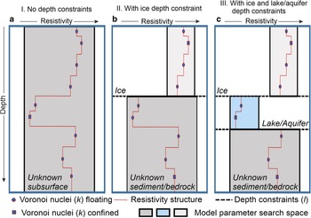
The depth constraints set the vertical extent of layer boundaries (l) within the model space (Fig. 2). For example, two layers could represent ice and subglacial material (Fig. 2b) or three layers could represent ice, a subglacial lake and subglacial material (Fig. 2c). The layer boundaries are used to define uniformly distributed prior distributions for resistivity, for each layer. For example, a high resistivity ice layer would most likely have layer boundaries set ~103–105 Ωm. The model is discretized using k piecewise constant functions based on Voronoi cells. Here, the confined nuclei are confined to their given layers but otherwise unconstrained in depth, and floating nuclei are unconstrained in depth and which layer they reside in (Fig. 2; Killingbeck and others, Reference Killingbeck, Livermore, Booth and West2018), where k is unknown with a uniformly distributed prior distribution between K min and K max. Where acceptable in terms of likelihood, the method always chooses simple (low k) models over complex models (high k). This means given a choice between a simple (e.g. thick layers with small resistivity changes) and complex (e.g. thin layers with large resistivity changes) model which provides a similar fit to the data, the simpler one will be favored. However, by adding layer boundaries, the preference for a smooth model in the inversion is relaxed, where sharp jumps in resistivity across a layer boundary are allowed and not penalized.
Illustration of MuLTI-TEM's model parameterization using Voronoi nuclei (floating and confined) comparing (a) a one-layer model, (b) a two-layer structure with ice overlying an unknown subglacial environment and (c) a three-layer structure with ice, a subglacial lake/aquifer and underlying unknown sediment/bedrock. We assume different ranges of resistivity within each layer, typical to that expected for the layer lithology. The boxes shaded in gray, blue and cream indicate the range of possible resistivity values for each layer. This figure is adapted from Killingbeck and others (Reference Killingbeck, Livermore, Booth and West2018).

The algorithm outputs probability density functions (PDFs) of resistivity for which we can analyze a variety of solutions such as the median (the value where 50% of the distribution lies), mode (peak of the distribution), average (mean of the distribution) or numerically best-fitting model. With access to the entire ensemble, detailed uncertainty analysis can also provide a measure of uncertainty for each depth calculated from either the std dev. or interquartile range. In this study, we used the median solution and interquartile range. The median solution was chosen because it closely overlapped with the mode solution (peak of the distribution), but did not include the unrealistic variations which can be observed in the mode solution when the distribution becomes wide and flat. For example, geologically unrealistic spikes can be observed in the resistivity-depth profile of the mode solution when the peak of the distribution is not distinctly defined. The average solution is not chosen as it smooths out the sharp layer boundaries at the ice–lake and lake–bedrock or lake–saturated sediment interfaces and, although the numerically best-fitting model has the lowest misfit to the data, these solutions generally have unrealistic resistivity-depth profiles and are not representative of the full PDF.
2.3. Deriving salinity of subglacial water from resistivity
Salinity is the quantity of dissolved salt content (e.g. sodium chloride, magnesium sulfate, potassium nitrate) in the water. The salinity of subglacial water can be measured in terms of the Practical Salinity Scale 1978 (PSS-78) (Perkin and Lewis, Reference Perkin and Lewis1980), which is recognized internationally as a standard measurement for salinity. It is noted that in 2010 a new standard for salinity was introduced called the thermodynamic equation of seawater 2010 (TEOS-10) (Millero and others, Reference Millero, Feistel, Wright and McDougall2008), advocating absolute salinity instead of particle salinity. However, the difference between the two measurements is negligible (a sample of seawater with chlorinity 19.37 ppt will have a PSS-78 practical salinity of 35.0 and TEOS-10 absolute salinity of 35.2 g kg–1) compared to the uncertainties that arise from TEM measurements.
The salinity of subglacial water can be inferred from resistivity profiles using Fofonoff and Millard's (Reference Fofonoff and Millard1983) internationally recognized conductivity to salinity conversion. This conversion directly relates the temperature, pressure and conductivity of the water to its PSS-78 practical salinity (Fig. 3), detailed further in the Supplementary material. The conversion has been calibrated with laboratory measurements within the temperature range −2 to 35°C, pressure range 0–10 000 decibars and practical salinity range 2–42. Temperatures, pressures and salinities outside these boundaries are therefore estimates which fit the calibrated relationship trend line that has been extended to these outer boundaries. Laboratory measurements have been conducted on practical salinities <2 and >42, where modified relationships have been applied (e.g. Hill and others, Reference Hill, Dauphinee and Woods1986; Poisson and Gadhoumi, Reference Poisson and Gadhoumi1993). However, the difference between these modified calibrated conversions and Fofonoff and Millard's (Reference Fofonoff and Millard1983) conversion is, also, negligible (on the order of 10−3) compared to the uncertainties that arise from TEM measurements.
(a) Pore fluid PSS-78 practical salinity as a function of bulk electrical resistivity and porosity of sediments. Bulk resistivity was computed using Archie's Law (Eqn (4)) with exponent m = 1.5 temperature −14.5°C and pressure 657 dbars. (b) Sensitivity testing m for m = 1, 1.3, 1.5, 1.8 and 2 with constant porosity (0.2), temperature (−14.5°C) and pressure (657 dbars). (c) Sensitivity testing temperature for T = 0, −5, −10, −14.5 and −20°C with constant porosity (1), m (1.5) and pressure (657 dbars). (d) Sensitivity testing pressure for P = 10, 300, 657, 800 and 1000 dbars with constant porosity (1), m (1.5) and temperature (−14.5°C). Here, the tortuosity factor (a) is 1 for all plots.

TEM methods are sensitive to the bulk resistivity of the subsurface. This quantity depends on the resistivity of the pore fluid and mineral grains and can be computed from a mixing law. Archie's Law (Archie, Reference Archie1952) is a commonly used approximation that predicts the bulk (measured) resistivity (ρ) from the pore fluids resistivity (ρ f), fractional porosity (Φ) and cementation factor (m) as

In Eqn (4) m represents the combined effect of the pore network, connectivity and permeability, with values for porous sediment ranging between 0.3 (low porosity) and 3 (high porosity) (Glover, Reference Glover2016). The term a is the tortuosity factor used to correct for variations in compaction, pore structure and grain size, with values ranging between 0.5 and 1.5 (Glover, Reference Glover2016). This formulation works well for porous sediments (Archie, Reference Archie1952) and fractured bedrock (Brace and Orange, Reference Brace and Orange1968). However, it is assumed that (1) no electrical conduction occurs within the rock grains and (2) Archie's Law does not account for the conduction of clay minerals. Several other mixing laws and modified versions of Archie's Law were developed to account for contributions from additional conduction processes (e.g. Hashin and Shtrikman, Reference Hashin and Shtrikman1962; Sen and others, Reference Sen, Goode and Sibbit1988; Glover, Reference Glover2010; Revil and others, Reference Revil2014). Most of these laws introduce additional factors into their estimation which increases the uncertainty of the petrophysical modeling (Mollaret and others, Reference Mollaret, Wagner, Hilbich, Scapozza and Hauck2020). Therefore, in this study, we use Archie's Law (Eqn (4)) while recognizing its inherent limitations.
Figure 3 shows the relationship between resistivity and PSS-78 practical salinity using the conductivity to salinity conversion (Fofonoff and Millard, Reference Fofonoff and Millard1983) and Archie's Law, highlighting the resistivity differences between fresh, brackish and brine water. Figure 3 also shows the sensitivity to porosity (Fig. 3a), m (Fig. 3b), temperature (Fig. 3c) and pressure (Fig. 3d). For example, in Figure 3a, a salinity of 1 psu can be explained by a resistivity of 15 Ωm with porosity 1 or 15 000 Ωm with porosity 0.01, where temperature, pressure and m are constant. In Figure 3b, 1 psu can be explained by a resistivity of 75 Ωm where m = 1 or 380 Ωm where m = 2, where temperature, pressure and porosity are constant. In Figure 3c, 1 psu can be explained by a resistivity of 10 Ωm at 0°C or a resistivity of 20 Ωm at −20°C, where porosity, pressure and m are constant. Finally, in Figure 3d, 1 psu can be explained by a resistivity of 15.7 Ωm at 10 dbs or a resistivity of 16.2 Ωm at 1000 dbs, where porosity, temperature and m are constant.
Here, we present the development of the MuLTI-TEMP algorithm to additionally derive the salinity of the subsurface fluids. The conductivity to salinity conversion (Fofonoff and Millard, Reference Fofonoff and Millard1983) and Archie's Law are applied to each resistivity-depth model within the ensemble of the posterior distribution (Supplementary Fig. S1). This outputs an additional PDF of PSS-78 practical salinity, provided that a prior distribution of porosity can be reliably estimated, for example, from nearby borehole measurements or detailed seismic velocity analysis (e.g. Wyllie and others, Reference Wyllie, Gregory and Gardner1956). A prior distribution of pressure and temperature is also required for the conductivity to salinity conversion; this can be obtained from borehole measurements or modeling, for example, using a 1-D steady-state advection–diffusion model. In this study, we use a Gaussian distribution to randomly sample each petrophysical parameter (temperature, pressure, cementation factor and porosity) from a prior mean and std dev.; however, this can be changed to a uniform or skewed distribution with depth, depending on the observed data.
3. One-dimensional synthetic study
3.1. Synthetic models
We use a variety of 1-D and 2-D synthetic models to highlight the strengths and limitations of TEM methods in a glacial environment and to validate the ability of MuLTI-TEMP to resolve a known subsurface structure. In this section, we discuss the 1-D synthetic models used in this study, which are extended to 2-D in the next section. Our synthetic models are based on the recent discovery of a hypersaline lake beneath the Devon Ice Cap in the Canadian Arctic (Rutishauser and others, Reference Rutishauser2018), where the ice is up to ~800 m thick. Here, the solute for the brine is hypothesized to be derived from an underlying evaporate-rich sediment unit called the Bay Fiord Formation, primarily dolomite, containing interbedded salt sequences consisting of 98% halite (Mayr, Reference Mayr1980; Harrison and others, Reference Harrison, Lynds, Ford and Rainbird2016). We model three different subglacial water scenarios under an 800 m-thick layer of ice, including:
• a 10 m-thick hypersaline lake (model A; Fig. 4a),
• a 10 m-thick saturated sediment layer with hypersaline pore fluid (model B; Fig. 4b),
• and a 10 m-thick hypersaline lake underlain by saturated sediment with decreasing porosity (model C; Fig. 4c).
Schematic 1-D synthetic models (hypothesized from Mayr, Reference Mayr1980), bulk resistivity and porosity for models: (a) A, (b) B and (c) C. Resistivity of the hypersaline lake and pore fluid was derived from the Practical Salinity Scale (PSS) 1978 (Perkin and Lewis, Reference Perkin and Lewis1980) using a salinity of 150 psu at −14.5°C and 657 dbars. The bulk resistivity of brine saturated sediments was derived from Archie's Law using m = 1.5.

The ice and bedrock resistivity values were estimated from previous polar EM studies (e.g. Mikucki and others, Reference Mikucki2015), at 10 000 and 1000 Ωm, respectively. The bedrock in our synthetic examples is modeled on that expected under Devon Ice Cap, primarily dolomite with interbedded halite sequences. Both dolomite and halite have high resistivities (≥1000 Ωm) and therefore the TEM method will not be sensitive to the individual lithologies within the bedrock. The lake and saturated sediment resistivity values were derived from Fofonoff and Millard's (Reference Fofonoff and Millard1983) conversion and Archie's Law. The resistivity of the hypersaline lake and pore fluid (ρ f), 0.16 Ωm, was derived assuming a salinity of 150 psu at −14.5°C and 657 dbars, representative of that expected under the Devon Ice Cap (Rutishauser and others, Reference Rutishauser2018). A cementation factor of 1.5, generally representative of porous (0.1–0.4) dolomite, was used in Archie's Law to derive the bulk resistivity of the porous brine saturated sediments in models B and C (Figs 4b, c).
Synthetic TEM responses were calculated from the 1-D models using the open-source Leroi forward modeling algorithm (CSIRO and AMIRA, 2019). The simulated TEM survey configuration assumes a 25 A current flowing in a square transmitter with a receiver in the center. In this study, we simulate the transmitter waveform from the Geonics TEM-67 system. This system has a fixed number of timegate channels which are recorded during the measurement period; here we set the number of channels to 30. A base frequency (1/T) is used to set the transmitter period (T) and the timegates are used to record the received voltage during the measurement period (T/4) (Fig. 1b). These timegates are automatically spaced to fill the whole measurement period. In this section, we analyze the TEM response using the base frequencies: 30 Hz (timegate 0.006–7.8 ms), 7.5 Hz (timegate 0.03–31 ms) and 3 Hz (timegate 0.08–78 ms). Figure 5 shows the TEM responses for four transmitter square sizes: 100 × 100 m, 250 × 250 m, 500 × 500 m and 1000 × 1000 m, using these base frequencies (30, 7.5 and 3 Hz). An estimate of the noise floor for ground-based TEM systems is assumed to be ~1 nV (Geonics, 2012; Killingbeck and others, Reference Killingbeck, Booth, Livermore, Bates and West2020).
Synthetic TEM responses for all models ((A) black, (B) red and (C) magenta) using four transmitter square sizes: 100 × 100 m, 250 × 250 m, 500 × 500 m and 1000 × 1000 m (x-axis), and the base frequencies 30, 7.5 and 3 Hz (y-axis), with 25 A current.

Firstly, we describe the forward problem and explain the shape of the TEM responses observed. For all synthetic models, at early times and the highest frequency (<10−1 ms; 30 Hz), the measured decay of the secondary EM field is relatively fast, corresponding to the 800 m-thick resistive ice layer present in all models. In the middle time range (10−1 to 101 ms; all base frequencies), the decay of the secondary magnetic field through the conductive lake (models A and C) is much slower (shown by the flat curves at 10−1 ms), due to larger secondary currents flowing in the conductive lake, compared to the less conductive saturated sediments (model B). At late times and the lowest base frequency (101 to 102 ms; 3 Hz), the measured decay of the secondary EM field increases corresponding to the underlying, less conductive, bedrock. Each base frequency is sensitive to a distinct depth range in the subsurface. Lower base frequencies result in later measurement times and increased DOI. In our examples, Figure 5 shows that multiple base frequencies are required to measure the full shape of the TEM signal, achieving a high resolution while maximizing the DOI.
Secondly, we discuss the effect of increasing the transmitter loop on the signal-to-noise ratio. As the transmitter loop increases, the received voltage of the signal increases (Eqn (2)). For transmitter loop sizes ≥500 × 500 m, using 25 A current, all transients for models A, B and C are above the background noise level (blue dashed line in Fig. 5) for all times. This is consistent with the maximum DOI for a 500 m loop on top of a resistive subsurface (Fig. 1c) and a suitable survey design to use for our synthetic models of the Devon subglacial hypersaline lakes.
3.2. Priors and parameters for MuLTI-TEMP inversion
We now consider applying MuLTI-TEMP to the 500 m × 500 m transmitter loop TEM responses for synthetic models A, B and C (Fig. 4). The base frequencies 7.5 and 3 Hz are chosen, as they target the TEM response corresponding to the subglacial lake and saturated sediments beneath the resistive ice layer (Fig. 5). We note a Bayesian joint inversion of all base frequencies could also be applied. However, to highlight the range of depth sensitivities of each base frequency, we performed the synthetic inversions individually. Also, by using a single TEM response, the inversion seeks a simpler solution. In our case, this results in an inversion model that is closer to the synthetic models and provides a better fit to the observed data. With this in mind, we therefore show the results from the individual inversions in the manuscript and Supplementary material. We add random noise to the TEM responses by using a simplified noise model consisting of 7.5% relative Gaussian noise applied to all time gates. For all base frequencies, any data points <1 nV (the estimated noise floor) were removed.
To highlight the benefit of using depth constraints, MuLTI-TEMP was run three times as follows:
(i) without any depth constraints (Fig. 2.I),
(ii) with a depth constrained base-ice layer (Fig. 2.II),
(iii) and with depth constrained base-ice and base-lake layers, or base-saturated sediment for model B (Fig. 2.III).
In II and III, the depth of the base-ice and base-lake horizons is fixed and their associated uncertainty is assumed negligible compared to the depth uncertainty in the TEM inversion. This is generally the case when using airborne radar to map ice thicknesses, where the vertical resolution of airborne radar through ice can be on the order of tens of meters, <5% of the total ice thickness (Rodriguez-Morales and others, Reference Rodriguez-Morales2013). Likewise, when using seismic measurements to map subglacial lake thicknesses, the vertical resolution can be on the order of 2 m, e.g. the imaging resolution of seismic data collected over Subglacial Lake Whillans (SLW) (Horgan and others, Reference Horgan2012). The inversions were run using the resistivity ranges shown in Supplementary Table S4, and a maximum depth of 1000 m. σ was set to 7.5% of the observed data. A single Markov chain was used in all inversions with 0.5 million iterations, to directly compare the posterior distribution from one chain for all three inversion tests (I, II and III). Most Bayesian inversions require multiple chains to obtain a fully converged solution, usually when no additional constraints on the model space have been applied. However, by using additional information from multiple datasets in MuLTI-TEMP, it was found that in most cases just one chain was required to obtain a fully converged solution which can be tested efficiently by running separate chains and comparing the solution output. The Markov chain is initialized with a randomized model from the prior distribution and run for a burn-in period. Here, we use a burn-in period of 10 000, 2% of the number of iterations, although this value is user-specific. After the burn-in period, the Markov chain is presumed independent of the initial condition and statistics of the chain are recorded from then on. The likelihood of a proposed model was calculated and only models with acceptable likelihoods were added to the chain, and applied in the next iteration as the current model; if a proposed model was not accepted, the existing model was retained as the current model. The acceptance criteria are detailed in Killingbeck and others (Reference Killingbeck, Livermore, Booth and West2018), Eqn (8). The prior distributions of the petrophysical parameters (temperature, pressure, cementation factor and porosity) were defined using the 1-D synthetic models (Fig. 4), with std dev. ±4°C (estimated from Rutishauser and others (Reference Rutishauser2018) modeled basal ice temperatures), ±4% of the pressure (estimated from the ice thickness uncertainty in the airborne radar measurements presented in Rutishauser and others (Reference Rutishauser2018)), ±10% of the cementation factor and ±10% of the porosity.
3.3. Results
Figures 6–8 show the results of the three inversion methods (I, II and III) applied to data generated from synthetic models A, B and C, respectively. In all figures, the first plot on the left shows the posterior distribution of the TEM responses accepted in the model ensemble compared to the observed (synthetic) data and its uncertainty (σ) applied in the inversion process. Next, we show the posterior distribution of resistivity comparing the median solution (black line) with the known synthetic model (red line). Finally, the furthest right plot shows the normalized least-squared misfit for each iteration, calculated from Eqn (3) and normalized by the number of data points (upper plot) and the posterior distribution of the number of Voronoi nuclei (lower plot). In the text to follow, we discuss each model's results sequentially, starting with model A.
1-D inversion results for model A (I) with no depth constraints, (II) depth constrained base-ice and (III) depth constrained base-ice and base-lake. (a) Comparison of synthetic data (black dots) and uncertainty tolerance with the posterior distribution of TEM responses for 3 Hz base frequency. (b) Posterior distribution of resistivity, comparing the median solution (black line) with the synthetic model (red line). (c) Normalized least-squared misfit for each iteration, see Tables S5 for detailed values (upper plot) and the posterior distribution of the number of nuclei (lower plot).

1-D inversion results for model B (I) with no depth constraints, (II) depth constrained base-ice and (III) depth constrained base-ice and base-sediment. (a) Comparison of synthetic data (black dots) and uncertainty tolerance with the posterior distribution of TEM responses for 7.5 Hz base frequency. (b) Posterior distribution of resistivity, comparing the median solution (black line) with the synthetic model (red line). (c) Normalized least-squared misfit for each iteration, see Tables S5 for detailed values (upper plot) and the posterior distribution of the number of nuclei (lower plot).

1-D inversion results for model C (I) with no depth constraints, (II) depth constrained base-ice and (III) depth constrained base-ice and base-lake. (a) Comparison of synthetic data (black dots) and uncertainty tolerance with the posterior distribution of TEM responses for 3 Hz base frequency. (b) Posterior distribution of resistivity, comparing the median solution (black line) with the synthetic model (red line). (c) Normalized least-squared misfit for each iteration, see Tables S5 for detailed values (upper plot) and the posterior distribution of the number of nuclei (lower plot).

For model A, the hypersaline subglacial lake scenario, Figure 6 shows the results from the inversion of the 3 Hz TEM response and Figure S2 shows the results from the 7.5 Hz TEM response. In Figure 6, all three inversion methods converge around the synthetic model's known resistivity structure, whereas in Figure S2, only the constrained inversion methods, II and III, identify the true lake's resistivity structure. In Figure 6, inversion method I, with no depth constraints, the lake is identified at 820 m depth (compared to 800 m depth in the synthetic model) with a resistivity of 0.4 Ω.m (compared to 0.16 Ωm in the synthetic model). The posterior distribution is more spread out compared to methods II and III, where multiple clusters of accepted models are shown ~820 m depth, 0.3 Ωm, and 850 m depth, 0.5 Ωm. Inversion method II introduces a constraint on the ice thickness. This enables the depth of the hypersaline lake to be identified accurately at 800 m; however, the resistivity of the lake is still slightly underestimated, 0.3 Ωm compared to 0.16 Ωm of the synthetic model. Inversion method III, which applies a constraint on the ice thickness and the base–lake interface, is successful in recovering the true thickness and resistivity structure of the lake. Here, the median solution matches the synthetic model in the lake.
For model B, the saturated sediment scenario, Figure 7 shows the results from the inversion of the 7.5 Hz TEM response and Figure S3 shows the results from the 3 Hz TEM response. In Figure 7, the 7.5 Hz TEM response measures the received voltages from the ice (0.01–0.1 ms), sediment (0.1–1 ms) and bedrock (1–10 ms) layers, whereas the 3 Hz TEM response, shown in Figure S3, only measures the received voltages from the sediment (0.1–1 ms) and bedrock (1–10 ms) layers. However, all three inversions (I, II and III) show similar results for both the 7.5 and 3 Hz TEM responses. Inversion method I identifies an 80 m-thick, conductive (16 Ωm) body at ~790 m depth. Inversion method II, which introduces a constraint on the ice thickness, identifies a 60 m-thick, conductive (12 Ωm) body at 800 m depth. Results from inversion I and II highlight a common issue with TEM inversions, exhibiting its sensitivity to conductance rather than layer thickness or conductivity alone (Section 2.2), allowing for ambiguities in the final solution. By not constraining the base–sediment interface, a thicker, more resistive layer with the same conductance as the synthetic model (5 Siemens) has fit the observed data within its uncertainty tolerance (the normalized misfit for all inversions, I, II and III, is ~1, Fig. 7c and Table S5). This limitation can be amplified by the Bayesian method we use in MuLTI-TEMP, where the algorithm always prefers a smooth model (low number of layers and small resistivity change) over a complex model (large number of layers and large resistivity change). This limitation is removed by using additional constraints in the inversion, as shown in inversion method III.
Finally, for model C, the subglacial lake and saturated sediment scenario, Figure 8 shows the results from the inversion of the 3 Hz TEM response and Figure S4 shows the results from the 7.5 Hz TEM response. In Figure 8, the 3 Hz TEM response captures the ice–lake interface, at 0.1–0.3 ms, and the sediment–bedrock interface, at 10–30 ms. Results from inversion I identify a ~20 m-thick, conductive (0.35 Ωm) body at 840 m, with a resistive bedrock increasing from 400 to 2000 Ωm. Inversion method II also identifies a ~20 m-thick, conductive (0.35 Ωm) body at 830 m depth, with a more conductive bedrock, increasing from 1 to 500 Ωm. Inversion III shows a tight posterior distribution, which matches the synthetic model to 875 m depth. After 875 m, the posterior distribution widens and the median solution strays from the synthetic model. This example demonstrates some limitations with the TEM method: it cannot discriminate between small differences in resistivity that are less than one order of magnitude and the method could potentially find it difficult to accurately image resistive bodies under thick conductive bodies.
For all models, the posterior distributions of resistivity show that the TEM method resolves conductive structures more accurately than resistive ones, shown by the tighter PDF over the conductive lake and saturated sediment layers compared to the resistive ice and low porosity bedrock layers. Also, all inversion methods (I, II and III) have a normalized misfit converging ~1 (Figs 6c, 7c, 8c and Table S5), showing all solutions fit the observed data to within their error tolerance, σ. These examples highlight that the TEM method can accurately identify a complex surface resistivity structure, such as a conductive hypersaline lake under thick resistive ice; however, the process requires multiple constraints and prior information to accurately steer the inversion toward a reliable solution, mitigating ambiguities and non-uniqueness in the final result.
Figure 9 shows the posterior distributions of salinity output from inversion methods II and III for all synthetic models. The left plot shows the mean and one std dev. of porosity input to MuLTI-TEMP and the right plot shows the posterior distribution of salinity, comparing the median (black) and synthetic (red) solutions. For model A, inversion II, the resistivity of the hypersaline lake is slightly overestimated, 0.3 Ωm compared to 0.16 Ωm (Fig. 6). This causes an underestimation in the median salinity solution, with 75 psu compared to 147 psu (Fig. 9). In inversion III, the resistivity and salinity of the lake are accurately recovered. For model B, inversion II, the salinity of the pore fluids is underestimated due to the overestimation of resistivity and thickness in the saturated sediments (Fig. 7). Here, the salinity of the pore fluids of the synthetic model lies well outside the posterior distribution of salinity estimated from the inversion (Fig. 9). In inversion III, the salinity is accurately estimated where the correct resistivity of the saturated sediments is determined. Finally, for model C, in inversion II, the salinity of the lake is not estimated because the conductive body is identified at 830 m depth, not 800 m depth which would match the prior porosity model used. Where salinity has been estimated, >840 m depth, the posterior distribution of salinity equals the prior distribution, and no reliable estimate of salinity can be made. In inversion III, by adding the base lake depth constraint, the salinity is accurately recovered to 875 m depth thus increasing the depth resolution of the inversion.
Petrophysical 1-D inversion results for models A, B and C (II) depth constrained base-ice and (III) depth constrained base-ice and base-lake/sediment. Left plot: mean and one std dev. of the prior distribution of porosity input to MuLTI-TEMP. Right plot: the posterior distribution of salinity, comparing the median and true solutions.

4. Two-dimensional synthetic study
4.1. Subglacial lake example 1
In this section, the synthetic inversions are extended to consider 2-D resistivity models. The MuLTI-TEMP code was used to invert multiple independent 1-D synthetic soundings along a synthetic 2-D line, with measurement points spaced at 500 m intervals. A 500 × 500 m transmitter loop and the TEM survey configuration presented in Section 3.2 were used in this study.
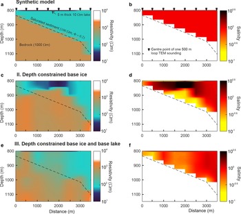
The first 2-D example uses a synthetic model with a similar structure and resistivity to that presented in Key and Siegfried (Reference Key and Siegfried2017) of SLW, West Antarctica. The model (Fig. 10a) consists of an 800 m-thick ice sheet (10 000 Ωm), underlain by a thick saturated sediment layer (100 Ωm), underlain by fractured bedrock (1000 Ωm), with a 2 km-wide, 5 m-thick (10 Ωm) subglacial lake. Additionally, in this study, we have assigned the salinity of the lake and pore fluid (1 psu) associated with the sedimentary structure using the conductivity to salinity conversion (Fofonoff and Millard, Reference Fofonoff and Millard1983) and Archie's Law, assuming a water temperature of −0.5°C (similar to that expected under SLW), pressure 657 dbars (equivalent to the hydrostatic pressure under 800 m-thick ice), cementation factor of 1.5 and porosity 0.2 within the saturated sediment layer (Fig. 10b). Key and Siegfried (Reference Key and Siegfried2017) used their 2-D synthetic model to test the ability of passive magnetotellurics (MT) and frequency domain electromagnetics to image near-surface sedimentary structures (e.g. a thin subglacial lake), and to image deeper groundwater. Here, we test the TEM method's ability to recover a 2-D subsurface structure where only multiple 1-D soundings are available, and to evaluate the potential of TEM to estimate the salinity of the subglacial water.
(a) 2-D subglacial lake synthetic model, overlaid by 800 m-thick ice (10 000 Ωm), and its (b) pore fluid salinity. (II) Depth constrained base-ice inversion's (c) median resistivity solution and its (d) estimated pore fluid salinity median solution. (III) Depth constrained base-ice and base-lake inversion's (e) median resistivity solution and its (f) estimated pore fluid salinity median solution.

Eight 1-D synthetic soundings were computed along the 2-D line with a spacing of 500 m using the Leroi forward modeling algorithm and base frequencies 7.5 and 3 Hz (Fig. S5). We inverted the 7.5 Hz TEM responses, as they measured the received voltages from the ice, sediment and bedrock layers, highlighted in Figure S5a. Again, following our previous notation, two inversion tests were run where in inversion II the base–ice interface was constrained (Figs 10c, d), and in inversion III the base–ice and base–lake interfaces were constrained (Figs 10e, f). Figure 10c shows that the unconstrained inversion recovers the lateral position of the lake, the thickening trend of the sediment package and the presence of underlying resistive bedrock. However, as in Figure 7, if the lake thickness is not constrained, a smoother model (~50 m thick with resistivity 50 Ωm), with the same conductance (~1 Siemens), is obtained. The model fits the observed data to within the data errors, but is different to the true model where the lake was 5 m thick with resistivity 10 Ωm. This causes the salinity of the lake to be underestimated and pore fluid salinity of the sediment directly beneath the lake to be overestimated (Fig. 10d). When the base–lake interface was constrained, the inversion recovers the true lake resistivity and salinity (10 Ωm and 1 psu) and the thickening trend of the sediment package beneath (Figs 10e, f). We note that beneath the lake, the sediment–bedrock boundary is not as sharp as in the true model; this is most likely caused by non-uniqueness (Section 2.2) which is discussed in the uncertainty analysis below. With actual field geophysical data, a quantitative uncertainty analysis will be required to identify which results are reliable and which are uncertain.
With access to the posterior distributions of resistivity and salinity from MuLTI-TEMP, quantitative uncertainty analysis along the 2-D line can be performed by calculating the interquartile range, between the 25th and 75th quartile, of the PDF at each depth. These uncertainties are plotted in Figure 11 for the two inversion tests. A high uncertainty in the solution is identified by a large, wide range (red) and low uncertainty is identified by a small, tight range (turquoise). Figures 11a and b show a high uncertainty (~100 Ωm) in resistivity in the depth range 850–900 m. These depths correspond to the resistivity increasing from ~50 to ~1000 Ωm (Fig. 10c), a good indication that this layer boundary is uncertain in inversion method II. Figures 11c and d show, in general, much smaller uncertainties (~10 Ωm) in the results from method III.
Quantitative uncertainty analysis for the (II) depth constrained base-ice inversion and (III) depth constrained base-ice and base-lake inversion. (a) and (c) Estimated uncertainty of resistivity. (b) and (d) Estimated uncertainty of salinity. The uncertainty was derived from the interquartile range, between the 25th and 75th quartile, of the PDF at each depth.

4.2. Subglacial lake example 2
The second 2-D example considers a more complex synthetic model with the same structure as example 1, but including a hypersaline lake (147 psu), based on the subglacial lake complex under Devon Ice Cap detailed in Section 3.1, and an imposed decrease in porosity with depth in the underlying groundwater system with a constant pore fluid salinity of 147 psu (Figs 12a, b). The hypothetical change in porosity could represent sediment compaction with depth.
(a) 2-D hypersaline lake synthetic model, overlaid by 800 m-thick ice (10 000 Ωm), with (b) lake and pore fluid salinity. (III) Depth constrained base-ice and base-lake inversion result with (c) median resistivity solution and (d) estimated pore fluid salinity median solution. (e) Estimated uncertainty of resistivity and (f) salinity derived from the interquartile range, between the 25th and 75th quartile, of the PDF at each depth.

Eight 1-D synthetic soundings were computed along the 2-D line with a spacing of 500 m using the Leroi forward modeling algorithm and base frequencies 7.5 and 3 Hz (Fig. S6), and inverted using MuLTI-TEMP. In this example, we inverted the 3 Hz TEM responses, as the measured received voltages from the hypersaline lake, sediment and bedrock layers are well above the background noise level, highlighted in Figure S6b. Both base–ice and base–lake interfaces were constrained in the inversion and the median solutions were analyzed (Figs 12c, d), along with an estimate of their uncertainty (Figs 12e, f). Figures 12c and d show that the TEM method recovers the conductive hypersaline lake and hypersaline pore fluid of the sediment layers with porosity 0.2 relatively accurately (to within one order of magnitude; highlighted in turquoise in Figs 12e, f) and estimates the salinity of the subglacial water relatively accurately (125–150 psu compared to the known synthetic salinity of 147 psu). Also, where there was no hypersaline lake at soundings 0 and 500 m, the synthetic model was recovered accurately and the uncertainty was within one order of magnitude. However, the inversion does not recover the gradual decrease in porosity with depth, in particular ≤0.1 porosity and the uncertainty beneath the sediment layer with porosity 0.2 is relatively high, between one and two orders of magnitude.
Both 2-D synthetic models presented here show TEM methods can image conductive bodies in the subsurface accurately. However, the depth resolution of TEM methods is limited under conductive bodies, i.e. hypersaline systems, and thus additional constraints of the subsurface structure beneath these bodies are required. In particular, MT methods could add valuable insights and constraints to the deeper resistivity structure in these environments, discussed further in the next section.
5. Discussion
The synthetic modeling in this study demonstrates that a ground-based TEM system using a large transmitter loop of 500 m × 500 m with 25 A current can detect and map subglacial water under polar ice sheets 800 m thick. Furthermore, this ground-based method could be used with larger transmitter loops, e.g. 1000 m × 1000 m, and currents (>25 A) which could potentially map subglacial water under regions of the ice sheets thicker than shown in this study (>1 km). The results from our synthetic inversion tests demonstrate that TEM methods are good at resolving conductive bodies. If additional constraints are available for the depth of interfaces, for example, from radar, seismic or borehole measurements, the conductive bodies are even more accurately resolved. This is ideal for mapping saline subglacial lakes, differentiating between saline and fresh pore fluid and characterizing zones of high porosity saturated sediment and low porosity bedrock. However, the TEM method may not be able to reliably discriminate between small differences in resistivity that are less than one order of magnitude (Fig. 8). In addition, the TEM method, alone, has limited depth resolution beneath conductive bodies, as highlighted in the 2-D synthetic example 2 (Fig. 12). Some of these limitations could be mitigated with additional knowledge of local geologic structures from active-source seismic data, which could further constrain the inversion. Improvements could also come from combining TEM with other EM methods. For example, passive EM methods, such as MT (which can image under thick ice sheets, >1 km), would be able to image deeper into the subglacial environment because they can use low-frequency, natural EM signals (~0.01–10 000 Hz). TEM and MT methods could be directly combined in a joint inversion approach since they are both sensitive to the subsurface resistivity structure. The near-surface ambiguities of MT methods could be mitigated by the relatively fine-scale resolution of TEM methods and deep structural ambiguities of TEM methods could be mitigated by the relatively large-scale depth resolution of MT methods.
Here, we have used the inversion tool MuLTI-TEM, which combines a probabilistic Bayesian approach with external depth constraints to mitigate ambiguous, non-unique solutions found in conventional TEM inversions. In this study, we have further developed MuLTI-TEM to a new version called MuLTI-TEMP with additional petrophysical analysis for applications with large ground-based systems, outputting a posterior distribution of salinity of the subglacial water. The Bayesian framework provides a robust quantitative uncertainty analysis of any chosen model at all depth levels. However, MuLTI-TEMP is a 1-D inversion algorithm and assumes a 1-D Earth, it does not currently invert for 2-D models, and does not take into account any 2-D (or 3-D) horizontal depth variations that may be present at late times. We have demonstrated in our 2-D examples that horizontal resistivity structure can be accurately resolved by inverting multiple independent 1-D soundings along a survey line. Although, to improve the spatial resolution and structure of the final 2-D model, in particular between soundings, additional spatial fusing methods, such as Bayesian maximum entropy (JafarGandomi and Binley, Reference JafarGandomi and Binley2013), could be used for horizontally gridding the multiple 1-D soundings. The Bayesian maximum entropy method could incorporate the different uncertainties associated to each 1-D resistivity profile, calculated from their PDFs, instead of applying a linear interpolation, when horizontal gridding along the 2-D line.
The additional petrophysical analysis applied in MuLTI-TEMP uses the conductivity to salinity conversion presented in Fofonoff and Millard (Reference Fofonoff and Millard1983) and Archie's Law. Archie's Law assumes there is no electrical conduction present within the rock grains and works well for porous sediment and fractured bedrock. However, it must be used with care if materials that exhibit surface conduction are present, such as clay, because surface conduction effects are not accounted for in Archie's Law (Worthington, Reference Worthington1993). With this in mind, TEM methods therefore cannot distinguish between subglacial water and conductive clays with similar resistivity values. This limitation can be addressed by using additional methods, such as active seismic, where changes in elastic properties may be greater than electrical conductivity enabling identification of the different subglacial materials. Furthermore, additional geochemical information from water and sediment samples from borehole measurements, for example, of groundwater chloride content, could enable mapping of groundwater chloride concentration as shown in Delsman and others (Reference Delsman2018), and detailed inferences on water residence time, brine sources and geochemical processes could be made (e.g. Michaud and others, Reference Michaud2016).
We recognize that we do not present any field data in this paper, and only consider synthetic data. However, this study highlights the potential of ground-based TEM methods for characterizing subglacial water bodies and their salinities under thick ice sheets. The study shows that TEM works best with constraints from radar and seismic. Therefore, when planning a ground-based survey, e.g. seismic, over a subglacial lake, the TEM method should also be considered to provide additional information on the water properties that seismic and radar cannot provide alone. The key survey requirements include a large transmitter loop, high current, thorough synthetic testing of survey design options and reliable estimates of background electrical noise levels.
6. Conclusions
Subglacial water can be detected, mapped and characterized using EM methods, which are sensitive to the resistivity structure of the subsurface. In this study, we have investigated the use of ground-based TEM methods for quantifying conductive subglacial water under resistive polar ice sheets. We present the recently developed Bayesian inversion MATLAB tool MuLTI-TEMP for deriving the salinity of subglacial water using Archie's Law and standard conversions of conductivity to salinity. We have investigated a variety of 1-D and quasi 2-D synthetic resistivity models based on a potential hypersaline lake under Devon Ice Cap in the Canadian High Arctic to illustrate how ground-based TEM methods could be used in an ice-sheet environment, where the ice is 800 m thick. MuLTI-TEMP incorporates independent depth constraints from, for example, seismic or radar measurements to limit the solution space, reducing ambiguity in the final resistivity profile. MuLTI-TEMP outputs posterior distributions of resistivity and salinity with depth, enabling a wide variety of statistics to be analyzed along with a quantitative uncertainty analysis. Here, we have shown that TEM methods resolve conductive bodies accurately, are suitable for mapping subglacial lakes and sediment saturated with hypersaline pore fluid, and provide their associated salinity. However, we also highlight that the depth resolution of TEM methods can be limited beneath deep, conductive bodies and therefore additional improvements could come from combining TEM with passive MT methods, where ambiguities in the TEM can be mitigated by the greater depth of exploration that is possible with MT.
Supplementary material
The supplementary material for this article can be found at https://doi.org/10.1017/jog.2021.94.
Data Availability
MuLTI-TEMP can be accessed at: https://zenodo.org/record/4446266 doi: 10.5281/zenodo.4446266. MuLTI-TEMP uses the Leroi algorithm of the CSIRO and AMIRA project P223F; CSIRO and AMIRA, 2019 and the Fofonoff and Millard's Reference Fofonoff and Millard1983 conductivity to salinity conversion algorithm, salinity.m, written in MATLAB by Edward T Peltzer, MBARI in 2007.
Acknowledgements
This research is part of the SEARCHArtic project funded by the W. Garfield Weston Foundation. Alison Criscitiello, Ashley Dubnick and Anja Rutishauser are thanked for their suggestions, comments and support with this research and manuscript. CD was supported by the Natural Sciences and Engineering Research Council of Canada (NSERC RGPIN-03761-2017) and the Canada Research Chairs Program (CRC 950-231237).


 Open access