

1. Introduction
The mass-balance cycle of avalanching glaciers (the concept of avalanching glaciers generalizes the concept of hanging glaciers; a definition is given in section 2) is characterized by a periodic or occasional release of ice by break-off mechanisms. Although relatively rare, icefalls or ice avalanches may pose a severe threat to humans, settlements and infrastructures. In the European Alps, one of the worst events of this kind occurred in 1965 in Switzerland, when a large part of the terminus of Allalingletscher broke off, killing 88 employees of the Mattmark dam construction site (Reference Röthlisberger and KasserRöthlisberger and Kasser, 1978; Reference Röthlisberger and KasserRöthlisberger, 1981; Reference Raymond, Wegmann and FunkRaymond and others, 2003). Ice avalanches which drag snow, water and/or rock can increase in size and have long run-out distances. The most destructive events of this kind on record occurred at Huascarán in the Peruvian Andes in 1962 and 1970 (e.g. Reference Morales ArnaoMorales Arnao, 1971; Reference BrowningBrowning, 1973; Reference LliboutryLliboutry, 1975; Reference Plafker, Ericksen and VoightPlafker and Ericksen, 1978; Reference PatzeltPatzelt, 1983): In 1962, a large snow and ice avalanche traveled 16 km into the Santa valley, destroying nine villages and killing more than 4000 people. In 1970, an earthquake triggered another ice avalanche; the estimated volume amounted to 107–108m3 (about ten times greater than the 1962 disaster). The city of Yungay was severely affected and more than 20 000 people were killed.
Following these tragic events, interest in the instability of avalanching glaciers grew within the alpine glaciological community. Descriptions or physical theories relating to these events were proposed (Reference LliboutryLliboutry, 1968; Reference Röthlisberger and KasserRöthlisberger and Kasser, 1978; Reference Röthlisberger and KasserRöthlisberger, 1981). In 1973, Weisshorngletscher which posed a threat to the village of Randa, Valais, Switzerland, was the subject of the first successful icefall prediction, by Reference FlotronFlotron (1977) and Reference Röthlisberger and KasserRöthlisberger (1981). Since then, approximately 16 avalanching glaciers have been investigated, some of them after a catastrophic event, others within the context of consulting work or research programs.
Inhabitants of endangered zones often have difficulty in recognizing, or are reluctant to acknowledge, the potential threat of ice avalanches. There can be physical reasons for this difficulty. Very large ice avalanches have a return period on the order of one generation, too long a time-span for the inhabitants to remain fully alert to the danger. Moreover, due to climatic variations, some avalanching glaciers undergo rapid changes leading either to isolated catastrophic events, or to new situations with no historical precedent. There can also be non-physical reasons for ignoring the threat. Reference HeimHeim (1932) described psychological mechanisms leading inhabitants to disregard signs of an impending catastrophe. Experts may come to be disbelieved after raising false alarms with their interpretations of observations, which are often based on previous experience and intuition.
Direct measurements on steep, heavily crevassed and avalanche-endangered glaciers are difficult to perform, and therefore often sparse and fragmentary, and difficult to interpret. They are usually carried out after clear signs of destabilization have been observed, so the conditions prevailing before an unstable state are uncertain. The factors responsible for the destabilization of large ice masses are the fracture behavior of ice and the stresses in the fracture zone. However, the physics of the ice fracture and the feedback mechanisms between crevassing, ice deformation and load distribution are complex and mostly unknown. Lack of theory and sparse measurements make an accurate stability assessment difficult.
In this paper, the instability of avalanching glaciers is discussed as follows. Section 2 proposes a definition of avalanching glaciers and classifies them according to different criteria, which allow a primary appreciation of the danger inherent in these glaciers. Section 3 summarizes observations and measurements of icefalls performed on glaciers in the European Alps. According to the proposed classification and the reported observations and with the help of the theory of ductile crevassing and numerical simulations of the fracture in avalanching glaciers, the mechanisms leading to the destabilization of ice masses and the recurrence of icefalls are analyzed in section 4. In section 5, knowledge of the calving mechanisms allows us to validate a method which has been traditionally used to forecast icefalls. The disaggregation of unstable ice masses, which can limit the accuracy of a forecast, is examined in section 6. A synthesis of the paper is presented in section 7.
2. Definition and Classification
The definition of avalanching and hanging glaciers is not clear-cut. According to Reference SharpSharp (1988), we define calving as the ice wastage by shedding of large ice blocks from a glacier edge, and calving glaciers as glaciers that lose mass by calving. We define dry calving glaciers as calving glaciers that are not in contact with a water body. To exclude dry calving processes occurring on flat margin surfaces, we define avalanching glaciers as dry calving glaciers lying on a steep slope (a slope which is sufficient to allow debris to fall away from the calving zone) or terminating on a bedrock cliff. The definition excludes glaciers with unstable seracs falling on the glacier itself, since these do not lead to mass loss. A hanging glacier is an avalanching glacier with particular properties, and is defined below.
Identification of avalanching glaciers is sometimes difficult: some exhibit very few icefalls; variations of climatic conditions induce glacier changes (advance, retreat, cooling, warming), which can modify the stability conditions, i.e. the occurrence of calving.
In this section, we propose a classification of avalanching glaciers, which is summarized in Figure 1. Avalanching glaciers can be classified according to the ratio between the unstable area (where calving occurs) and the total area of the glacier. Two limiting cases can be distinguished, which we propose to call ‘terrace’ and ‘ramp’ glaciers.
Summary of the classification of the avalanching glaciers. The classifications Terrace/Ramp and Balanced/Unbalanced refer to the type of avalanching glaciers, and the division Wedge/Slab to the type of fractures. The unstable ice masses are depicted in gray. The mass-balance regime is indicated with arrows.

Terrace glaciers are avalanching glaciers with a bedrock characterized by a significant increase in slope at the glacier margin, which induces calving. The calving area is small relative to the glacier size. These avalanching glaciers can present a high frequency of icefalls (recurrence in some years), since the fracture zone is constantly supplied by the upstream glacier area and the ice-release volumes are small compared to the total glacier volume.
Ramp glaciers are avalanching glaciers lying on a uniform, even, steep bed, which leads to major instabilities. The calving area represents a significant portion of the glacier. The unstable part is supplied principally by direct snow accumulation. Therefore, after a failure, a long period (usually one to several decades) is required to reach another critical state.
Terrace and ramp glaciers are either in a ‘balanced’ or ‘unbalanced’ mass-balance regime:
Balanced avalanching glaciers. Under constant climatic conditions, these glaciers can attain a steady-state geometry without releasing ice by calving. Usually the occurrence of icefalls does not follow a cycle.
Unbalanced avalanching glaciers. Under constant climatic conditions, these glaciers must release, by calving, a substantial quantity of ice to maintain a finite size geometry. A cycle or pseudo-cycle of icefalls is thus observed. The icefalls recur over a period longer than a hydrologic year, i.e. several years to decades. Therefore, the notion of steady-state geometry does not strictly exist in this context. For avalanching glaciers, the notion of steady state should be related to an entire icefall cycle.
We define hanging glaciers as unbalanced avalanching glaciers. The two classifications above refer to characteristics of the whole glacier. Following Reference HaefeliHaefeli (1965), a third classification criterion is introduced, referring to the fracture process. Two main processes are considered, which are related to the bedrock topography in the calving zone:
The slab fracture occurs on steep bedrock slopes. The unstable ice mass is a slab, which represents either a large part of the glacier (ramp glaciers), or the glacier margin (terrace glaciers). Very large ice volumes (typically 105-106m3) can be released. In the case of temperate basal ice, failures have been observed for slopes steeper than 25° (see section 3). For cold basal ice, the bedrock slope does not exceed 45°. Reference AleanAlean (1985) observed a dependence of the critical slope (the slope for which the glacier is unstable) on the altitude: the higher the altitude, the steeper the critical slope. This dependence was related to the correlation between the fraction of ice frozen to the bed (the basal adhesion of the glacier) and the altitude.
The wedge fracture occurs because of a topographic discontinuity in the glacier bedrock, usually forming a cliff. This discontinuity limits the extension of the glacier and leads to calving when ice is transferred beyond this limit. When calving occurs, the glacier margin forms an ice cliff. The unstable ice mass is an ice lamella, which breaks off from the glacier edge. The basal ice can be cold or temperate. The typical ice-release volume is 103–105m3. According to previous classifications, wedge fracture occurs only for unbalanced terrace glaciers, since the ice mass transferred beyond the bedrock cliff must calve (unbalanced avalanching glacier) and the bedrock beneath the calving area presents a discontinuity (terrace glacier).
This last classification is based on a two-dimensional representation of the bedrock topography (in a vertical plane parallel to the ice flux). Three-dimensional effects, such as the arched structure of the glacier front (Reference OttOtt, 1985) or the concavity or convexity of the bedrock, can interfere with the fracture modes. Moreover, an avalanching glacier can calve consecutively under both modes of fracture. The interaction between the two fracture modes is not considered in the following, and the avalanching glaciers listed are classified with respect to the dominant mode.
The above classifications provide primary indications of the probability, the recurrence and the volume of icefalls. Unbalanced avalanching glaciers, unlike balanced glaciers, always lead to icefalls. For terrace glaciers, the rate of recurrence of major icefalls can be high (a few years);it is on the order of one decade for ramp glaciers. Wedge fractures have smaller ice-release volumes than slab fractures.
3. Observations of Avalanching Glaciers
In the Alps, only a few avalanching glaciers have been investigated so far. Table 1 gives an overview of these glaciers. The best-documented are presented in this section according to the classification proposed in section 2. They are also mapped in Figure 2.
Map of the avalanching glaciers. The squares, triangles and circles refer, respectively, to the glaciers, the mountains to which they belong and the main cities of the region. Aig. stands for Aiguille and gl. for glacier.

Documented avalanching glaciers in the Alps. All glacier characteristics refer to the calving zone. T, terrace glacier; R, ramp glacier; B, balanced avalanching glacier; U, unbalanced avalanching glacier; s, slab fracture; and w, wedge fracture

3.1. Terrace glaciers
3.1.1. Balanced avalanching glaciers
3.1.1.1. Slab fracture: Allalingletscher
Allalingletscher is a balanced temperate terrace glacier with slab fracture (Fig. 3a). Since the mid-1950s, after a significant retreat, the glacier has terminated on a rock slope of about 27°. On 30 August 1965, 2 × 10⁶m3 of ice broke off from the glacier terminus, fell down the rock slope and buried a construction site located 1 km below the glacier, killing 88 employees. An intensive glaciological study and monitoring program was undertaken after this catastrophe to safeguard the rescue operation and the construction work, and to analyze the causes of the avalanche. The investigations showed that the ice avalanche occurred during a phase of enhanced motion resulting from an intense slip of the glacier tongue (Reference Röthlisberger and KasserRöthlisberger, 1981); the fracture occurred along an arched line. Since this event, it has been established that such an active phase occurs periodically (every 1–3 years), alternating with a quiescent phase. Accelerations are still noticeable in the quiescent phase, but remain an order of magnitude smaller than during the active phase. The active phase begins in summer and ends in late autumn (Fig. 3b). It seems to depend on the presence of meltwater, but also on the ice mass distribution along the longitudinal profile of the tongue (Reference Röthlisberger and KasserRöthlisberger, 1981). Although an active phase is necessary for the front of the tongue to break, this does not explain why an icefall occurred in 1965, rather than during another active phase before or after this date. After 1965, Allalingletscher advanced to a stable state until the mid-1980s and then retreated again. Around 1996, the geometry of the glacier terminus was similar to that in 1965, and a repetition of the slip-off event could be expected during an active phase. In July 2000, an ice volume of 1 × 10⁶m3 broke off (Fig. 3a). Thanks to the safety measures, no damage was done.
(a) Tongue of Allalingletscher with the arch line (dotted line) of the fracture as observed after the 2000 event (photograph by F. Funk-Salami). (b) Variation in velocity vs time of the glacier tongue during three active phases of enhanced ice motion (measured by Reference Röthlisberger and KasserRöthlisberger, 1981). The 1965 curve corresponds to the deceleration measured immediately after the accident (see text). The 1966 and 1967 curves correspond to the acceleration measured during these two years. The fit of both curves is performed with Equation (4).

3.1.2. Unbalanced avalanching glaciers
3.1.2.1. Slab fracture: Balmhorngletscher
This glacier is located in the Bernese Alps, Switzerland. After a significant retreat during the 1930s (Reference Raymond, Wegmann and FunkRaymond and others, 2003), the orographic right part of the glacier formed an unbalanced terrace glacier with slab fracture (Fig. 4);the ice there is temperate. Reference RöthlisbergerRöthlisberger (1987) analyzed numerous calving events from this glacier and observed that icefalls are related to a phase of enhanced motion (active phase) and to the mass distribution along the length profile of the tongue. He discussed the phase shift observed between the glacier melting cycle and the active-phase cycle of the unstable zone. He explained this phenomenon by a progressive disorganization of the drainage system caused by enhanced sliding during the active phase, which traps the subglacial water flowing under the unstable glacier part.
Balmhorngletscher (hanging glacier). The dotted line delimits the unstable zone (photograph by E. Gyger, ~1940).

3.1.2.2. Wedge fracture: Eigerhängegletscher
Eigerhängegletscher is an unbalanced terrace glacier with wedge fracture, located on the west face of the Eiger, Bernese Alps, Switzerland (Fig. 5a). The glacier extends from 3500 to 3200ma.s.l., with a surface slope of 20° at the terminus. The maximum thickness is about 70 m. The glacier is temperate except in the vicinity of the front (Reference Lüthi and FunkLüthi and Funk, 1997). Reference Lüthi and FunkLüthi and Funk (1997) argue that the temperature distribution influences the global stability of the glacier, so that warming of the cold front can destabilize the entire glacier.
(a) Eiger west face with its unbalanced terrace glacier (arrow) (photograph by S. Bader, 1987). (b) Measured acceleration of the lamella in 2001 and its fit performed with Equation (4). The predicted failure time (corresponding to abscissa zero) is 18 August.
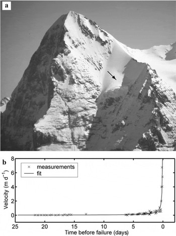
In 1990, a large crevasse was observed behind the glacier front. This crevasse destabilized a frontal ice lamella, which was threatening human settlements below the glacier. A theodolite-laser distometer was installed at a fixed position near the glacier, and three reflectors mounted on stakes drilled in the unstable ice mass were used to survey the movement of the lamella. Reference reflectors installed on a rock face close to the unstable ice mass allowed us to correct the influence of the meteorological conditions on the measurements. These corrections reduce the measurement errors to approximately 1 cm (see Reference Pralong and FunkPralong and others, 2005). The time of the breaking-off was estimated by selecting an empirical function (see Equation (4) below) to fit the progressive acceleration of the unstable ice mass (see section 5). The icefall of 105m3 occurred on 20 August, 3 days later than predicted (VAW, unpublished information). In 2001, the movement until failure of a smaller lamella was measured for scientific purposes, using the same method as in 1990 (Fig. 5b). The unstable ice chunk disaggregated progressively: several limited icefalls were observed during 1 week in mid-August 2001.
3.1.2.3. Wedge fracture: Gutzgletscher
Gutzgletscher, Bernese Alps, Switzerland, is a temperate unbalanced terrace glacier with wedge fracture. On 5 September 1996, 2 × 10⁵ m3 of ice avalanched down the 1000 m high west face of the Wetterhorn. The debris blocked a road, and the induced wind injured three people (Reference Margreth and FunkMargreth and Funk, 1999). Three years later a dangerous situation was recognized in time (Fig. 6a). A stake network installed on the lamella was monitored with the theodolite-laser distometer, in order to measure the motion of the unstable glacier part (Fig. 6b). A breaking-off was successfully predicted to within 1 day by applying the same method as for Eigerhängegletscher. The failure occurred on 14 August 1999.
Fig. 6. (a) Gutzgletscher (hanging glacier) with the unstable ice mass (dotted line) as observed in July 1999. (b) Measured displacement of the unstable ice mass and its fit performed with Equation (5). The observed failure time (corresponding to abscissa zero) is 14 August.

3.1.2.4. Wedge fracture: Mönchgletscher
The hanging glacier located on the south face of the Mönch, Bernese Alps, Switzerland, (Fig. 7a) is an unbalanced terrace glacier with wedge fracture. In 2001 the bedrock topography was determined from the drilling of six boreholes to the bed along two flowlines (Fig. 7a and b). The glacier lies on a large, uneven bedrock terrace (Fig. 7b). Temperature records in the boreholes showed that the glacier is temperate, except at the orographic right side close to the rear part of the glacier base (Fig. 7b), where the coldest measured temperature is —0.6 ± 0.05°C. This cold region does not influence the calving process, since it is of limited size and distant from the calving zone.
(a) Mönch south face with its unbalanced terrace glacier. The picture shows the relics of an ice avalanche which occurred on 5 July 1984 (photograph by J. Alean). The black dots show the location of the six boreholes. (b) Two longitudinal profiles of the glacier corresponding to the two series of boreholes in (a). The left and right profiles correspond to the left and right dots in (a). The vertical dotted lines show the location of the holes along the profiles. The measured depth of the glacier at the location of the holes is reported. Elsewhere the bedrock geometry is estimated. The measured temperature is reported for each borehole. The circles show the location of the measurements along the holes. (c) Measured acceleration of the lamella in 2000, and its fit performed with Equation (4). The observed failure time of the main icefall (corresponding to abscissa zero) is 27 July. The observed partial failures are marked with vertical bars (3 and 25 July). Note the abrupt velocity decrease after the first partial failure.

The detachment of two lamellas (in 2000 and 2001) was monitored by surveying the positions of stakes installed on them. Figure 7c shows the results of measurements of the 2001 event. Each of the two lamellas broke off in several pieces. Three partial icefalls were observed during the 2000 event. The volume of each icefall was approximately 4 × 10⁴ m3. The remaining part of the lamella (6 × 10⁴ m3) disaggregated progressively (VAW, unpublished information). Two significant icefalls were observed in 2001, with a volume of approximately 103m3. They separated from a 105m3 lamella, which disaggregated progressively in the course of 1 year. According to observations over the past 20 years, only a few lamellas fell in one major icefall (VAW, unpublished information, and further observations by the authors). The majority of the lamellas disaggregated, leading to a series of small breaking-off events.
3.2. Ramp glaciers
3.2.1. Balanced avalanching glaciers
3.2.1.1. Slab fracture: Ghiacciaio Superiore di Coolidge
Until the 1950s, this small temperate glacier, located in the Cottiennes Alps, Italy, presented a frontal cliff and formed an unbalanced terrace hanging glacier. Until the beginning of the 1970s, the glacier retreated and thinned (the frontal cliff disappeared) and the surface slope increased to 35°. It then formed a balanced ramp glacier. In 1986 a transverse crevasse was observed in the upper part of the glacier. On 6 July 1989, the ice mass located below the transverse crevasse destabilized and slipped over its bed. The volume of the icefall amounted to 2 × 10⁵ m3. It is presumed that a period of intensive rainfall resulted in a significant increase in basal water pressure, which lifted the glacier and caused the failure (Reference Dutto, Godone and MortaraDutto and others, 1991). Figure 8a and b show the glacier before and after its collapse.
Ghiacciaio Superiore di Coolidge (a) before and (b) after the 1989 event. Photographs by M. Vazan (1987; archives of Italian Glaciological Committee, Turin, Italy) and R. Tibaldi (1989; archives of Craveri Civil Museum, Bra, Italy). The height of the ice cliff after failure was 35 m.

3.2.1.2. Slab fracture: Altelsgletscher
Altelsgletscher, Bernese Alps, Switzerland, is a polythermal balanced ramp glacier. On 11 September 1895 it was the scene of the largest known icefall in the Alps (5 × 10⁶ m3; Reference Raymond, Wegmann and FunkRaymond and others, 2003), caused by weakening of the contact at the ice/rock interface. This possibly resulted from the thawing of a frozen zone at the glacier front after several exceptionally warm summers (Reference Röthlisberger and KasserRöthlisberger, 1981). The shape of the fracture line showed a regular parabolic arch, with a span width of 580 m (similar to that of the 1980 icefall at the Iliamna volcano, Cook Inlet, Alaska, USA; Reference AleanAlean, 1984). Figure 9a and b show Altelsgletscher before and after the collapse. A similar event was reported in 1792 (Reference Raymond, Wegmann and FunkRaymond and others, 2003), but no precise information is available on this.
Altelsgletscher (a) before and (b) after the 1895 event. Photographs by P. Montandon (1894 and 1895; archives of Alpine Museum, Bern, Switzerland).

3.2.2. Unbalanced avalanching glaciers
3.2.2.1. Slab fracture: Aiguille ďArgentière north face
The north face of Aiguille ďArgentière is situated in the Valais Alps, Switzerland, with the summit at 3900ma.s.l. and the bottom at approximately 3000ma.s.l. A series of 25 photographs was assembled to document the changes of the north face during the last century. Some are presented in Figure 10a. The series gives an illustration of the temporal and spatial evolution of an unbalanced cold ramp glacier clinging to the center of the face. On the lower right part of the face, an unbalanced terrace glacier leans on a rock spur. This terrace hanging glacier did not vary substantially during the last century. The ramp hanging glacier, by contrast, showed remarkable activity. Just before the beginning of the 20th century it covered the upper and middle part of the face; four years later, it had almost disappeared. Between 1925 and 1930 it covered approximately the same area as in 1899, then it completely disappeared again. A 1942 photograph shows a face quasiuniformly covered by firn and ice, but with two small irregularities at the top. Until the end of the 1940s, these irregularities grew slowly, then they increased more rapidly and in 1953 formed a single ramp hanging glacier. Between 1953 and 1958 the ramp and terrace hanging glaciers merged, and then the lower part of the ramp glacier progressively disaggregated. From the beginning of the 1970s, this ramp glacier was no longer connected to the terrace glacier and occupied only the upper part of the face. The position of the ramp glacier did not significantly evolve until the mid-1990s, after which it progressively disappeared as its front retreated. In 2003 a small hanging glacier was observed at the top of the face.
(a) Evolution of the north face of Aiguille d’Argentière over more than one century. Photographs (in archives of VAW, Zürich, Switzerland, unless stated) by M. Roch (1899), unknown author (1903; archives of M. Colonel, Servoz, France), unknown author (1930), A. Roch (1942), H. Fredenhagen (1949), S. Pfister (1953), E. Vanis (1958), O. Laternser (1961), F. Valla (1976), P. Sandmeyer (1990) and C. Vincent (2003). (b, c) Annual sum of positive degree-days (b) and annual water equivalent snowfall precipitation above –5°C (c) for the face of Aiguille d’Argentière. The circle and the points differentiate values derived from daily and monthly (due to lack of data) meteorological data. The horizontal solid (dashed) lines at the top of each plot show the period when the ramp glacier extends (reduces).

To analyze possible influences of variations in accumulation and ablation on the observed cycles of the ramp glacier, daily temperature and precipitation records from the nearby Grand-Saint-Bernard meteorological station (located 20km from Aiguille ďArgentière, under a similar climatological regime) are considered (MeteoSwiss data). The temperature data have been corrected with a lapse rate of 6.1 × 10~3°Cm–1 (Reference Urfer, Gensler, Ambrosetti and ZenoneUrfer and others, 1979) (considering a mean glacier altitude of 3500 m) to take into account the difference in altitude. The annual sum of positive degree-days is used as a proxy for annual ablation (e.g. Reference BraithwaiteBraithwaite, 1995). The accumulation is approximated with the sum of the precipitation over 1 year at air temperatures between –5 and 0°C: only snowfall occurring above –5°C is assumed to accumulate on the steep face (Reference Kuroiwa, Mizuno, Takeuchi and ÕuraKuroiwa and others, 1967). We neglect the effects of wind on the accumulation, as well as positive feedbacks between accumulation, variation of glacier surface slope due to accumulation, ice motion, etc. (see section 4). The sum of the positive degree-days and the cumulated precipitation are presented in Figure 10b and c. Results throughout the observation period do not show a significant correlation between observed glacier changes and meteorological data. The disappearance of the glacier at the beginning of the 20th century and during the 1930s is not explained by a decrease in accumulation or by an increase in temperature. The two periods of growth around 1920 and during the 1950s are not explained by a reduction in ablation and precede by several years an increase in accumulation. Only the last two periods of disappearance (the 1960s and 1990s) can be related to climatic warming. Therefore, climatic conditions alone do not explain the long- and short-term variations in the glacier.
3.2.2.2. Slab fracture: Weisshorn east face
The Weisshorn east face is covered with a few unbalanced cold ramp glaciers located between 3800 and 4500ma.s.l. In winter, snow avalanches triggered by icefalls threaten the village of Randa located some 2500 m below the glacier, and traffic routes to Zermatt (Fig. 11). A compilation of historical events showed that Randa suffered repeated severe damage during past centuries (Reference Raymond, Wegmann and FunkRaymond and others, 2003).
Weisshorn east face with the threatening hanging glacier (arrow) as observed in autumn 1972 (photograph by B. Perren). The village of Randa and traffic routes are visible in the valley (bottom of picture).

In 1972, an unstable ice chunk of 500 000 m3 was observed and gave cause for alarm. To estimate its failure time, velocity measurements of the unstable ice mass were performed for the first time by Reference FlotronFlotron (1977) and Reference Röthlisberger and KasserRöthlisberger (1981). Flotron proposed an empirical function (see Equation (4)) to fit the measurements in order to predict the failure time. The measurements were interrupted 37 days prior to the collapse (the collapse occurred on 19 August 1973), after >250 days of monitoring (VAW, unpublished information). The failure occurred 2 weeks later than predicted. The volume of the falling ice mass was one-third of what was expected (only the frontal part broke off). Due to disaggregation of the glacier front, episodic icefalls of limited volume were reported as early as 3 months prior to the collapse (Reference Röthlisberger and KasserRöthlisberger, 1981). On the basis of aerial photographs, Reference Röthlisberger and KasserRöthlisberger (1981) estimated that the unstable ice mass started to accelerate in 1968, 5 years before breaking. He also reported two other major icefalls during the 20th century: between 1920 and 1928, and between 1959 and 1968.
3.2.2.3. Slab fracture: Grandes Jorasses hanging glacier
This unbalanced cold ramp glacier is located on the south face of the Grandes Jorasses, Mont Blanc Massif, Alps, Italy (Fig. 12a). In 1997, the opening of a transverse crevasse in the upper part of the glacier suggested possible destabilization of a significant part of the glacier (Fig. 12b). Six boreholes were drilled down to the bed, and temperature profiles were measured (Fig. 12b and e). At all of these places, the basal temperature was below the freezing point (below –1.6±0.4°C), precluding the possibility of an ongoing sliding process due to progressive basal warming. The glacier velocities were monitored using a stake network. Significant acceleration was observed between 1997 and 1998 (Fig. 12f). Unfortunately, the measurements were stopped 3 months prior to the break-off. During the period of observation, a dense fracture network was recognized at the base of the glacier (Fig. 12c). From mid-May 1998, the formation of a second crevasse, located approximately 10m below the existing crevasse, was observed. This crevasse opened very rapidly, and on 30 May 1998 the part of the glacier located below it collapsed (Fig. 12d). The fracture plane, parallel to the bedrock, was located approximately 10m above it. The detached volume amounted to approximately 2.5 × 10⁵ m3. Fortunately, the ice avalanche caused no damage.
Fig. 12. (a) Summit of Grandes Jorasses south face with its hanging glacier, January 1997. (b) Enlargement of the upper crevasse, January 1998. The numbers indicate the location of the boreholes. (c) Zone of fracture at the orographic left side of the hanging glacier. (d) Situation after June 1998 event (photographs by R. Cosson). (e) Temperatures and glacier thickness as measured in January 1998 at the location of the boreholes (see panel (b)). The vertical dotted lines show the location of the holes relative to the glacier front. The thickness of the glacier at these points is reported. The measured temperature is presented for each borehole. The circles show the location of the measurements along the holes. (f) Measured surface velocity at borehole 1. The observed failure time (corresponding to abscissa zero) is 30 May 1998. The measurement error amounts to 0.5 cm d–1. (g) Three stages of the simulated fracture process occurring in the hanging glacier. The black areas depict the location of the fractures (where damage reaches the value of the critical damage (Reference Pralong and FunkPralong and Funk, 2005)). Axes are related to the lower plot. The upper, middle and lower plots, respectively, correspond to 1.5 years, 4 months and 1 week before failure. Panel (a) corresponds to the first stage of the simulation, panels (b) and (c) to the second stage and panel (d) to the observed state of the glacier 1 week after the third simulation stage.

4. Calving Mechanisms and Recurrence of Icefalls
As observed in section 3, the destabilization of unstable ice masses from avalanching glaciers involves different calving mechanisms. In this section, with the help of the classification proposed in section 2, we analyze these calving mechanisms and then, with the results of this analysis, discuss the recurrence of icefalls.
4.1. Calving mechanisms
Destabilization processes, which lead to icefalls, depend on the fracture process of ice and on the stress in the fracture zone. The stress in the fracture zone is influenced by the glacier geometry, the ice density and the basal conditions. For avalanching glaciers, the stress in the fracture zone is usually less than a few bars (Reference IkenIken, 1977; Reference Lüthi and FunkLüthi and Funk, 1997; Reference Pralong and FunkPralong and Funk, 2005). At this stress magnitude, the ice fracture is a process of microcrack accumulation, with a characteristic timescale in the order of weeks (Reference VoitkovskiyVoitkovskiy, 1960; Reference Szyszkowski and GlocknerSzyszkowski and Glockner, 1986; Reference Mahrenholtz, Wu, Murthy, Sackinger and WadhamsMahrenholtz and Wu, 1992), and not a brittle fracture (Reference WeissWeiss, 2004; Reference Pralong and KnightPralong, 2006). The dynamics of microcrack closure is controlled by crack healing (Reference Derradji-Aouat and EvginDerradji-Aouat and Evgin, 2001; Reference Pralong and FunkPralong and others, 2005). No microcrack appears in the ice below a stress threshold (Reference Gold and ŌuraGold, 1967). To initiate microcrack accumulation, the stress in the fracture area must rise above the value of the stress threshold. This occurs through changes in glacier geometry and/or modifications of basal sliding conditions. The resulting positive feedback mechanism between damage (density of microcracks) and local stress distribution near the fracture, as well as the crack healing and the stress inhomogeneities, leads to a localization of the microcracks and the formation of a macroscopic fracture (e.g. crevasse) (Reference Pralong, Funk and Lüthi.Pralong and others, 2003; Reference Pralong and KnightPralong, 2006). The macroscopic fracture in ice is the mechanical reason for the destabilization of an ice chunk. In the following, this process is discussed for wedge and slab fractures.
4.1.1. Wedge fracture
Wedge fracture is initiated by an increase in the ice mass at the glacier front due to ice flow and snow accumulation. This increase induces higher longitudinal stresses and the opening of a frontal crevasse. This crevasse progressively separates an ice lamella from the rest of the glacier. Numerical simulations by Reference IkenIken (1977), Reference Pralong, Funk and Lüthi.Pralong and others (2003) and Reference Pralong and FunkPralong and Funk (2005) (see also Fig. 14) and observations after icefalls at the Mönchgletscher (Fig. 13) show that the frontal crevasse first opens and deepens due to tension forces. This mode of fracture occurs either in the calving zone or in the upstream stable glacier part during destabilization of a previous lamella. For this latter case, the crevasse is advected to the front by the glacier motion, then destabilization of the lamella proceeds by the development of a shearing fracture in the prolongation of the crevasse. This shearing fracture develops without deepening and enlarging of the crevasse. According to Reference Pralong and FunkPralong and Funk (2005), the acceleration of the lamella is dominated by the positive feedback between the depth of the fracture and the stress concentration at its tip. Once this fracture has reached the glacier front (usually at its base), the icefall occurs.
Front of Mönchgletscher (Fig. 7a) after a failure (2001 event). The shape of the fracture under tension (1) and under shearing (2) is visible.

Simulation of an ice fracture with different basal geometries: (a) vertical bedrock cliff and (b) inclined bedrock cliff at the glacier front. The black areas depict the location of the fractures (where damage reaches the value of the critical damage (Reference Pralong, Funk and Lüthi.Pralong and others, 2003)). The former simulation shows the formation of a secondary fracture in the middle of the unstable ice chunk, whilst the latter presents a homogeneous unstable chunk.

The ice flow in the vicinity of a cold glacier front is approximately constant seasonally. It can vary for temperate glaciers, due to the seasonal variation of basal sliding and water content in ice. The increase in the ice velocity induces a faster transfer of the unstable ice mass to the front, which increases the stresses more swiftly and thus shortens the period of the failure process. For temperate glaciers, the probability that a failure will occur during the melt season is higher. Both events observed at Gutzgletscher were reported at the end of summer. At Mönchgletscher, where the cold region is negligible, seven of the nine observed major icefalls occurred in summer or autumn (Table 2).
Dates of the Mönchgletscher main icefalls (Reference AleanAlean, 1985, and observations performed by the authors) located on the west side of the front. Series stands for the number of observed consecutive failures

4.1.2. Slab fracture in cold ice
Due to their shape and position, cold avalanching glaciers with slab fracture are principally subject to shear stresses. The longitudinal stresses are small in comparison. Therefore, the fracture develops in a plane located where the shear stress is maximum, i.e. near the glacier base. When the unstable zone reaches a critical thickness (it principally thickens due to direct accumulation), the shear stress overcomes the stress threshold for damage initiation and a fracture develops.
Since direct observations of the fracture process at the glacier base are not possible, we refer in the following to a numerical simulation of Grandes Jorasses (cold ramp hanging glacier). To simulate the fracture process, we apply the damage model of Reference Pralong and FunkPralong and Funk (2005). The bedrock geometry and ice temperature were determined from in situ measurements. The accumulation is estimated from observations. The simulation starts with a shallow glacier corresponding to the observed glacier geometry at the end of summer 2003. A crevasse in the upper part of the glacier appears 2.5 years before failure, as observed in nature (Fig. 12g, upper plot). It does not directly influence the stability of the avalanching glacier, but separates the steep part from the glacier summit. Approximately 250 days before failure, a shear fracture begins to develop in the steep part of the glacier, near the bed. It grows parallel to the bed, simultaneously over the whole fracture zone (Fig. 12g, middle plot). A few weeks before failure another crevasse develops rapidly downstream of the existing one (as observed in nature) and separates the unstable ice slab from the upper stable part (Fig. 12g, lower plot). Finally the icefall occurs.
The dense fracture network observed at the base of Grandes Jorasses is reproduced in the model by local damage accumulation. This accumulation is due to the large shear stresses at the glacier bed (approximately 1.5 bars) and leads to destabilization of the glacier. The position of the fracture plane over the bed is lower in the model than in nature. This difference may be associated with bedrock irregularities, which are not considered in the model. The progressive acceleration of the unstable ice mass, observed in the present simulation, seems to be related to the positive feedback between local stress in the plane of fracture and damage accumulation.
The formation of an upper crevasse, such as that first observed at Grandes Jorasses, is related to the increase in the bedrock slope and not to the destabilization process. Such a crevasse is therefore not necessarily observed on other cold ramp glaciers, which cling to a homogeneous face (e.g. Aiguille d’Argentière). According to the numerical results, the progressive acceleration occurring several years before the failure (Weisshorn) is related to the progressive thickening of the glacier due to snow accumulation and not to the destabilization process, which is concentrated over 1 year.
4.1.3. Slab fracture in temperate ice
The slab fracture in temperate ice occurs when basal drag decreases. The forces exerted by the unstable ice mass on the upstream stable glacier part increase drastically and lead to a tensile fracture. A shear fracture at the glacier base can usually be excluded, since the thickness and the slope of the unstable slabs (which do not usually exceed 20–30m thickness and 30° slope for temperate glaciers with slab fracture) do not induce enough stress to allow failure (Reference LliboutryLliboutry, 1968; Reference RöthlisbergerRöthlisberger, 1987).
Basal drag usually decreases due to the presence of meltwater at the glacier base, flowing in a drainage system affected by the enhanced ice motion (Allalin- and Balm- horngletscher). As claimed by Reference RöthlisbergerRöthlisberger (1987; see also Reference Iken and BindschadlerIken and Bindschadler, 1986), rapid sliding during an active phase induces the formation of cavities and simultaneously a progressive disorganization of the drainage system, which leads to undrained subglacial cavities under the unstable glacier part. It can reasonably be assumed that the increased area of these cavities enhances glacier sliding (Reference KambKamb, 1987). In that case, a positive feedback exists between cavity area and basal sliding which leads to the acceleration of the unstable slabs (Fig. 3b, 1966 and 1967 curves). For slab fractures in temperate ice, this feedback mechanism seems to govern calving. For Allalin- and Balmhorngletscher, where there were no variations in basal sliding, no icefalls were observed and the reduction of meltwater led to the deceleration of the unstable mass (Fig. 3b, 1965 curve). The acceleration of the unstable ice slab takes place over a few weeks. More rarely, the reduction of the basal drag occurs due to external disturbances, such as rapid water-pressure increase due to abundant liquid precipitation (Ghiacciaio Superiore di Coolidge) or warming of the basal layer due to an increase in air temperature (Altelsgletscher). The different timescales of the destabilization processes are noteworthy: destabilization due to rapid water-pressure increase occurs approximately over 1 day, the drainage feedback over 1 month and the warming of the basal layer over a few years. In all cases, the ‘natural’ adaptation (due to modification of the mass balance) of the glacier to reach a stable state lasts longer than the destabilization process, resulting in potential instability of these glaciers.
The unstable ice mass usually breaks along an arch line, reposing on two abutments on both sides of the unstable ice mass (Ott, 1985) (Figs 3a and 9b). This line is normal to the maximum principal stress acting in the ice. The ice mass located above this arch line is stable. It is retained by compressive forces applied on the lateral abutments. The ice mass below the arch line is potentially unstable. It holds on the ice above the arch line and generates tensile stresses. Due to ice flow through the line, the unstable ice mass (and therefore the tensile stresses) increases until failure occurs (Ott, 1985) or another stable regime is reached. The stability of the avalanching glacier depends not only on lateral abutments, but also on the bedrock roughness, which helps to stabilize the glacier (Allalingletscher). If these stabilizing factors are lacking, the whole avalanching glacier (or at least a large part of it) can break off (Ghiacciaio Superiore di Coolidge).
4.2. Recurrence of icefalls
Let us define an ice-release cycle as the time period T between two consecutive mass-balance minima (we consider here minima due to calving and not to seasonal melting or other ablation phenomena). Thus, we might introduce the total mass release R iot (i) (due to calving) during the cycle i as

q(t) is the net ice flux in the fracture zone, defined as being the ice flux flowing from the upstream stable part of the glacier in the fracture zone plus the mass balance into the fracture zone. ti is the time at the beginning of the cycle i. Equation (1) can then be rewritten as

where

is the mean net ice flux between the beginning of the cycles i and i + 1. The above relations are valid only if the position of the fracture line does not vary between successive ice-release cycles. This is the case for a glacier with wedge fracture (the fracture line is located behind the bedrock cliff) and cold glaciers with slab fracture (the fracture line lies near the glacier bed) since the fracture depends mainly on the bedrock topography, which is constant. On the other hand, the position of the fracture line of temperate glaciers with slab failure can be variable. The fracture process depends principally on stress increase due to basal sliding (which is not necessarily constant at each cycle), and not on topographic conditions.
4.2.1. Wedge fracture
In the case of wedge fracture, the geometry of the unstable ice mass is primarily constrained by the bedrock topography. Over successive release cycles, one might therefore expect R
tot to remain approximately constant if the glacier geometry (and especially the thickness of the glacier calving margin) does not vary. q principally depends on the basal sliding and the mass balance of the glacier. Under constant climatic conditions, q varies seasonally (due principally to variations of basal sliding and mass-balance regime in the fracture zone). Oscillations of ![]() (due to seasonal variations of q) decrease with T
–1. For all observed hanging glaciers with wedge failure, the period T was at least 2 years. Therefore, variations of
(due to seasonal variations of q) decrease with T
–1. For all observed hanging glaciers with wedge failure, the period T was at least 2 years. Therefore, variations of ![]() are small between successive release cycles. If climatic conditions change, q can vary. For example, the exceptionally warm summer of 2003 reduced the volume of the Mönch unstable ice chunk by melt. Therefore the mean net ice flux
are small between successive release cycles. If climatic conditions change, q can vary. For example, the exceptionally warm summer of 2003 reduced the volume of the Mönch unstable ice chunk by melt. Therefore the mean net ice flux ![]() decreased considerably. Under constant conditions, and according to Equation (2), the period T should not vary considerably for glaciers with wedge fracture, since R
tot and
decreased considerably. Under constant conditions, and according to Equation (2), the period T should not vary considerably for glaciers with wedge fracture, since R
tot and ![]() remain approximately constant. Observations at Mönchgletscher confirm this conclusion. During the 1980s and 1990s, the climatic conditions were approximately constant and the release cycle times were approximately 2 years (Table 2).
remain approximately constant. Observations at Mönchgletscher confirm this conclusion. During the 1980s and 1990s, the climatic conditions were approximately constant and the release cycle times were approximately 2 years (Table 2).
4.2.2. Slab fracture in cold ice
Since cold avalanching glaciers with slab fracture grow on a uniform bedrock slope, usually a face (Aiguille d’Argentière; Weisshorn), the dimensions of the calving zone are not limited primarily by the bedrock topography but by the fracture process. The total mass release, R
t0t, can therefore vary over successive cycles. Subcycles of ice release during a main cycle (Aiguille d’Argentière) may also make Rtot variable. Observed cold avalanching glaciers with slab fracture demonstrate ice-release cycles of one to several decades. During such a time period, accumulation on the unstable glacier part is significant and principally influences ![]() . The accumulation depends on the surface slope, which is itself affected by accumulation, ice motion and icefalls. The accumulation and thus
. The accumulation depends on the surface slope, which is itself affected by accumulation, ice motion and icefalls. The accumulation and thus ![]() are governed by complex feedback mechanisms. Under constant climatic conditions and over successive release cycles,
are governed by complex feedback mechanisms. Under constant climatic conditions and over successive release cycles, ![]() may therefore vary. According to Equation (2), no periodicity in the release cycles may be expected, since R
tot and
may therefore vary. According to Equation (2), no periodicity in the release cycles may be expected, since R
tot and ![]() are not constant and do not necessarily vary proportionally. Observations at Aiguille d’Argentière confirm this. Release cycle periods amounted there to 35 and 60 years, without being explained by climatic variations alone.
are not constant and do not necessarily vary proportionally. Observations at Aiguille d’Argentière confirm this. Release cycle periods amounted there to 35 and 60 years, without being explained by climatic variations alone.
4.3. Slab fracture in temperate ice
The slab fracture of temperate terrace glaciers is governed primarily by the seasonal variation of basal sliding. However, as observed at Allalin- and Balmhorngletscher, the slab failure depends on the mass transfer from year to year into the unstable part and on particular bedrock characteristics in the fracture zone. The period T is therefore not constant. For temperate ramp glaciers, the conditions favorable to an icefall are produced by external forcing disturbances, such as climatic variations or particular meteorological events: exceptional rainfalls (Ghiacciaio Superiore di Coolidge) or a succession of warm summers (Altelsgletscher). Since these disturbances are usually not periodic, these glaciers do not present regular release cycles.
5. Icefall Forecasting
Correct forecasting of large icefalls can prevent loss of life and damage to settlements and infrastructure in the hazard zones. At present, the most promising approach for such prediction is based on the regular acceleration of the unstable ice chunks prior to collapse. This section considers the accelerations measured on all the surveyed glaciers, and the calving mechanisms described, in order to validate and improve this forecasting method. Due to positive feedback mechanisms (described in section 4) the velocity of the unstable ice mass approaches a finite time singularity (Reference Sammis and SornetteSammis and Sornette, 2002);that is, theoretically the velocity increases to infinity at a finite time (forming a singularity) according to (e.g. Reference VoightVoight 1988):
where u(t) is the velocity at time t, u 0 is a constant velocity, t f is the time of failure and a u and m u are positive parameters characterizing the acceleration of the unstable ice chunk. The observed acceleration of ice chunks in the case of positive feedback between damage and stress (involved in wedge fracture and slab fracture in cold ice) is adequately described using Equation (4) (Reference IkenIken, 1977; Reference Röthlisberger and KasserRöthlisberger, 1981; Lüthi, 2003; Reference Pralong and FunkPralong and Funk, 2005; Reference Pralong and FunkPralong and others, 2005) (Figs 5b, 6b and 7c). Positive feedback between the surface of the undrained water cavities and the sliding, as assumed for slab fracture in temperate ice, can also be described by Equation (4). Figure 3b presents the fit of the acceleration measured by Reference Röthlisberger and KasserRöthlisberger (1981) at Allalingletscher. The correlation coefficients are 0.96 and 0.99 for the 1966 and 1967 curves, respectively. Equation (4) is widely used. It describes the fracture of materials such as rock, soil and high-performance metal alloys (Reference VarnesVarnes, 1983).
This characteristic dependence of velocity on time makes the forecasting of icefalls possible. Velocity measurements performed during the failure process are fitted with Equation (4); the velocity is then extrapolated and the failure is predicted when u → ∞, i.e. when t → t f. The first event to be successfully forecast using Equation (4) was the 1973 Weisshorn event (Reference FlotronFlotron, 1977; Reference Röthlisberger and KasserRöthlisberger, 1981). The authors subsequently made other accurate predictions for Eiger-, Gutz- and Mönchgletscher. The failure forecast, i.e. the determination of tf, can also be made using the integrated form of Equation (4):

where s(t) is the position at time t and s 0 is a parameter. The advantage of using Equation (5) instead of (4) for determining t f is that the measured positions s(t) can be used directly for the fitting procedure without differentiating the data to obtain u(t). During the derivation of s(t), the noise related to the measurements can hide the global trend. However, using Equation (5) requires an additional parameter (s 0) to be identified.
For slab fracture in temperate ice, acceleration is not necessarily followed by an icefall (in contrast to slab failure in cold ice and wedge failure, where acceleration always precedes a break-off). For example, between the 1965 and 2000 failures at Allalingletscher, 17 active phases with significant sliding (and therefore an acceleration; see Fig 3b) were observed but no collapse occurred. In those cases, the predictive method presented cannot reasonably be applied, so this mode of fracture is not further discussed in this section. Current knowledge is inadequate for making accurate forecasts of such phenomena.
The acceleration of unstable ice masses cannot be described by Equation (4) or (5) if strong external disturbances occur during the destabilization process, since they affect the feedback processes responsible for the failure. These disturbances differ according to the different types of fractures:
Wedge fracture. The positive feedback leading to failure occurs between damage and stress. The stress principally depends on the mass of the unstable ice chunk.
Therefore, variations of mass affect the destabilization. Increase of mass due to accumulation during the fracture process is usually negligible. However, ice loss (due to disaggregation; see below) and melting can considerably reduce the mass and retard the failure (Fig. 7c).
Slab fracture in cold ice. The positive feedback leading to failure also occurs between damage and stress. In cold avalanching glaciers with slab fracture, the longitudinal dimensions are larger than the vertical dimensions. Thus, the ice is principally subjected to shear stresses. Ice releases at the glacier front do not substantially change the shear stress at the glacier base and therefore do not perturb the fracture process.
By setting u 0 = 0, the velocity u at t = 0 nevertheless does not vanish. u(t = 0) then corresponds to the creep velocity of ice at the beginning of the fracture process, i.e. to the creep of ice without damage (e.g. Reference Mahrenholtz, Wu, Murthy, Sackinger and WadhamsMahrenholtz and Wu, 1992). u 0 is therefore a term which generalizes the description of the failure process by adding a constant velocity characterizing a uniform ice motion into the fracture zone. The value of this term depends on the type of fracture:
For wedge fracture, two types of motion are superimposed. The first motion type is the creep deformation due to shearing stresses, which occurs principally at the glacier base. The second motion type results from damage concentration at the glacier surface, which induces crevasse opening and acceleration. For wedge fracture, the damage accumulation is thus not directly coupled with glacier deformation. The acceleration process can therefore be described in a reference system, which moves with the independent velocity u 0 of the glacier. Equation (4) should be used with u 0 inferred from velocity measured at a point located on the upstream side of the frontal crevasse. The variations of surface velocities due to variations of basal sliding are thus taken into account.
For slab fracture in cold ice, the damage is localized at the glacier base. Since no sliding occurs, the fracture zone is not shifted. u 0 corresponds here to the ice deformation between the plane of fracture and the glacier surface, i.e. the ice deformation in the virgin ice (ice wihout damage).
6. Disaggregation
The global destabilization of an ice mass is induced by formation of a tensile fracture, which isolates the frontal ice mass from the glacier, or by development of a shearing fracture plane, which separates the ice slab from the bedrock. Beside these main fracture processes, subprocesses of fracture occur. They disturb the main destabilization process and make the prediction of the time of failure and the volume of the largest ice avalanche difficult. This section analyzes these subprocesses of fracture.
We propose the term ‘disaggregation’ for the separation of an unstable ice mass into smaller ice parts due to subprocesses of fracture. During a release cycle, the disaggregated part gives rise to successive icefalls, which occur at the front and the lateral faces of the unstable ice chunks. Such icefalls occur before or after a main failure. Compared to the ice volume of the main failure, the cumulated volume of pre-release is generally small, but can be very large for post-release (Mönchgletscher).
Disaggregation can be related to several factors. A numerical analysis using a damage model by Reference Pralong, Funk and Lüthi.Pralong and others (2003) shows that a variation in the bedrock cliff slope may or may not generate the disaggregation of the unstable mass (Fig. 14). This depends on whether the stress field in the calving zone is influenced by the bedrock geometry and whether the evolution of the damage in ice depends on the stress. Bedrock irregularities at the front of the glacier can thus trigger these secondary fractures. The crack healing limits the effects of disaggregation by reducing the crack density. This process is probably thermally activated (personal communication from J. Weiss, 2003), but is not quantified. Another factor that influences the disaggregation is the ductility of ice. The ductility increases with increasing temperature. The effects of healing and ductility cumulate. Therefore, a higher ice temperature causes lower disaggregation activity. The velocity of the unstable ice chunk also controls the disaggregation. If the chunk does not move, no disaggregation occurs. Rapid ice motion amplifies the inhomogeneity of the stress field created above bed disturbances and induces more cracks.
Disaggregation has been reported at Eiger-, Mönch-, Weisshorn- and Allalingletscher (no similar observations are available for other glaciers). The mass of the successive icefalls due to disaggregation during the 1973 Weisshorn event is evaluated on the basis of photographs taken by an automatic camera installed at a fixed position near the glacier (Reference Röthlisberger and KasserRöthlisberger, 1981). Figure 15a shows the estimated averaged ice-release rate ![]() (kgd–1) between two consecutive photographs as a function of time. The time is expressed by the difference t
f – t, where t
f is the observed time of failure. The ice-release rate due to disaggregation can be approximated by
(kgd–1) between two consecutive photographs as a function of time. The time is expressed by the difference t
f – t, where t
f is the observed time of failure. The ice-release rate due to disaggregation can be approximated by
(a) Release rate at Weisshorngletscher (hanging glacier). The observed failure time of the main icefall (corresponding to abscissa zero) is 19 August 1973. The fit is performed with Equation (6). (b) Release rate at Mönchgletscher (hanging glacier) (Fig. 7a). The fit is performed with Equation (6). The predicted failure time of the main icefall is 1 August 2003. The effective time of the main icefall can only be estimated (using the measured acceleration of the unstable ice mass (Reference Pralong and FunkPralong and others, 2005)) since the last sub-failure stopped the main failure process.

with ![]() 0 a constant release rate term and aR and m
R positive parameters characterizing the acceleration of the disaggregation process. The disaggregation at Mönchgletscher possibly follows the same law (Fig. 15b). Here daily photographs (also from an automatic camera) permit the observation of individual icefalls (stars in Fig. 15b) during a destabilization process (2003 event; see Table 2). The rate of the ice releases was calculated using the time-span between two consecutive falls. This relation cannot be validated for other glaciers due to a lack of data.
0 a constant release rate term and aR and m
R positive parameters characterizing the acceleration of the disaggregation process. The disaggregation at Mönchgletscher possibly follows the same law (Fig. 15b). Here daily photographs (also from an automatic camera) permit the observation of individual icefalls (stars in Fig. 15b) during a destabilization process (2003 event; see Table 2). The rate of the ice releases was calculated using the time-span between two consecutive falls. This relation cannot be validated for other glaciers due to a lack of data.
The parameter ![]() 0 can be associated with the ice-release rate related to the stable motion u
0 of the glacier. For
0 can be associated with the ice-release rate related to the stable motion u
0 of the glacier. For ![]() 0 ¼ 0, the parameter a
R is proportional to the total ice-release volume R
tot(i) during the cycle i. The value m
R is a measure of the disaggregation. m
R increases for decreasing disaggregation activity. mR → 0 corresponds to a maximum disaggregation activity with a constant release rate
0 ¼ 0, the parameter a
R is proportional to the total ice-release volume R
tot(i) during the cycle i. The value m
R is a measure of the disaggregation. m
R increases for decreasing disaggregation activity. mR → 0 corresponds to a maximum disaggregation activity with a constant release rate ![]() . mR → ∞ represents a minimum disaggregation activity: only one failure occurs at t = t
f.
. mR → ∞ represents a minimum disaggregation activity: only one failure occurs at t = t
f.
Let us express the release rate ![]() due to disaggregation as a function F of the velocity u of the glacier:
due to disaggregation as a function F of the velocity u of the glacier:
with u
0 being the constant velocity term in Equation (4) and ![]() 0 the constant release rate in Equation (6). By introducing
0 the constant release rate in Equation (6). By introducing
![]() –
– ![]() 0 for the disaggregation and u – u
0 for the velocity, only the influence of the unstable motion of the glacier is considered. Since Equations (6) and (4) are similar, one can write
0 for the disaggregation and u – u
0 for the velocity, only the influence of the unstable motion of the glacier is considered. Since Equations (6) and (4) are similar, one can write
with the parameters α and μ defined as
The parameter m R, which expresses the disaggregation activity, thus equals μ mu. The bedrock irregularities, the crack healing, the ice ductility and the velocity of the unstable ice mass have been identified as influencing the disaggregation, i.e. the value of m R. The first three factors are considered in μ, and the last one is characterized by m u.
To analyze Equation (8), let us suppose that the position of the glacier front is stable during a failure process, i.e. disaggregation exactly compensates the ice velocity at the front. Then the ice supply q at the glacier front corresponds to the ice release ![]() , i.e.
, i.e. ![]() (t) = q(t). The ice supply q can be approximated by
(t) = q(t). The ice supply q can be approximated by
The area A represents the surface of the glacier front, ρ is the mean ice density (averaged along the vertical axis) and λ u is the ratio of the mean velocity (averaged along the vertical axis) to the surface velocity normal to the glacier front. One can then write
Since this equation is also valid when ![]() is replaced by
is replaced by ![]() 0 and u by u
0, one obtains
0 and u by u
0, one obtains
Comparing this result with Equation (8), one concludes that for a fixed front, one has α = Ap λ u and μ = 1, i.e. α R = Aρ λ u a u and m R = m u. For terrace glaciers, the assumption of a fixed front is plausible since the position of the fracture is determined by the bedrock topography. Observations at Mönchgletscher (using a series of daily photographs) showed that when the front becomes too steep or exceeds the position of the bedrock cliff, small icefalls from the lamella occur. Note that this disaggregation is a discrete process. Only a few icefalls were observed (stars in Fig. 15b). If disaggregation is not very active, the front advances: the disaggregation does not compensate the ice flux q. In that case, μ > 1. If no disaggregation occurs, μ → 1 so that m R → ∞. Inversely, if disaggregation is very active, the front retreats and μ < 1.
Due to the finite time singularity of Equation (6), the total volume of icefall, until a short period prior to the main failure, represents a small amount of the volume of the unstable ice mass, unless disaggregation is significant. Close to the main failure, volumes of icefall can become significant. At that stage, disaggregation can strongly influence the fracture process by removing mass from the system, which can delay the main failure. Disaggregation can, moreover, separate the unstable chunk into a few smaller parts. The volume of the largest icefall can therefore be reduced considerably, making it difficult to forecast. This happens frequently and has been reported for the majority of avalanching glaciers.
7. Discussion
The successive failures of avalanching glaciers seem to have a random character. Observations have shown that despite similar conditions at the beginning of many ice-release cycles, each cycle evolves differently. As seen above, a numerical simulation (Fig. 14) has shown that small variations in the boundary conditions at the front of the glacier can influence the disaggregation process. Reference Pralong and FunkPralong and Funk (2005) described the large influence that some fracture parameters of ice have on the geometry of the unstable ice mass. Further numerical simulations performed with their model show that the failure time is sensitive to variations in fracture parameters. This behavior can be explained by considering Equation (4) describing the acceleration process. The time of failure t f is expressed as

with t an arbitrary time of the acceleration process. u(t) corresponds to the value of the velocity of the unstable ice mass at time t, i.e. to an initial condition of the velocity when t is considered to be the beginning of the fracture process. Figure 16 shows the sensitivity of t f to the initial condition u(t) and the parameter mu for the values of the 2001 Eigerhängegletscher failure (for this destabilization process tf is not sensitive to au, since the dependence on au is approximately linear: here m u ≈ 1). Since Equation (13) is non-linear, small variations of u(t) and mu strongly affect the value of tf. This effect is attenuated when t converges to tf. Considering Equation (6) instead of (4), and performing the same analysis, it appears that the disaggregation is also sensitive to initial conditions and parameter values.
Influence of the variation of (a) the exponent m
u and (b) the initial velocity u(t) on the time of failure t
f calculated with Equation (13). The parameters m
u and u(t) vary around reference values mu and u*(t) (vertical dotted lines) measured during the 2001 event at Eigerhängegletscher (Fig. 5b). ![]() is the difference between the time of failure t
f calculated with the different values of the parameters m
u and u(t) and the reference time of failure
is the difference between the time of failure t
f calculated with the different values of the parameters m
u and u(t) and the reference time of failure ![]() related to the measured reference parameters
related to the measured reference parameters ![]() and u*(t). The variations of Δ t
f depend on the time-span
and u*(t). The variations of Δ t
f depend on the time-span ![]() (in days in the legend) between the initial time t of the failure process and the time of failure
(in days in the legend) between the initial time t of the failure process and the time of failure ![]() corresponds to the variation of u(t) around the measured reference value u*(t). Note that the initial velocity u(t) evolves with time t, i.e. with
corresponds to the variation of u(t) around the measured reference value u*(t). Note that the initial velocity u(t) evolves with time t, i.e. with ![]() For the four values of
For the four values of ![]() the reference initial velocity u*(t) amounts to:
the reference initial velocity u*(t) amounts to:

In that way, small variations in ice properties, initial or boundary conditions seem to induce large variations of the icefall characteristics. Therefore, the time of rupture, the maximum release volume, the disaggregation activity or the number of post-releases cannot be predicted on the basis of past events or measured initial conditions. Moreover, a precise prediction only emerges when the time of the measurements approaches the time of failure. An accurate forecast must thus be based on ongoing measurements and observations. A prediction based on numerical simulations seems unrealistic, since neither the initial conditions (temperature and damage distribution in ice), nor the boundary conditions (basal sliding, bedrock irregularities), nor the ice parameters (ice-flow parameters and ice-fracture parameters) are precisely identified or measurable.
Disaggregation complicates the forecast of the breaking-off time for two reasons. First, the disaggregation process leads to the failure of secondary ice masses. These processes develop more quickly and their location is difficult to predict. Their corresponding volumes are usually small. Second, close to the main failure, these secondary icefalls significantly influence the destabilization process. The prediction of the volume of the largest icefall may be overestimated due to disaggregation of the ice chunk. The failure time of the unstable ice mass can also be delayed by partial failure. A temporal increase in disaggregation activity can be used to estimate the time of failure of the unstable ice chunk. A similar approach is applied to the prediction of earthquakes by considering the seismic events preceding a large quake (Reference Bufe and VarnesBufe and Varnes, 1993). For glaciers, this method should, however, be applied with restraint, since partial icefalls can be rare if disaggregation is less active.
For slab fracture in cold ice and wedge fracture, the intrinsic cause of the failure is the progressive formation of a fracture. For wedge fracture, the presence of a crevasse at the front is a good indicator of potential danger. However, the enlargement and deepening of the crevasse should not be used to estimate the stage of destabilization. Enlargement of the fracture depends not only on the motion of the unstable ice chunk, but also on the motion of the stable part of the glacier. Moreover, the final stage of destabilization does not occur through enlargement and deepening of the crevasse, but by propagation of a shearing fracture. For slab fracture in cold ice, the fracture processes are usually not observable and the formation of surface crevasses is not necessarily associated with the destabilization process. For slab fracture in temperate ice, the instability is related principally to the basal conditions. The risk of a major icefall is especially acute during an active phase of sliding. Nevertheless, the active phase is only one of the necessary conditions for the occurrence of a significant icefall.
Variations in climatic conditions are important for the stability of avalanching glaciers. Modification of the mass balance influences the total ice flux in the fracture zone and therefore affects the mean period between successive breakings-off. An increase in air temperature modifies the thermal conditions of the glaciers, which are of primary importance for cold avalanching glaciers, in terms of their stability conditions.
8. Conclusions
On the basis of observations and measurements performed on avalanching glaciers and of numerical simulations of fractures, the calving processes in avalanching glaciers and the recurrence of failures have been analyzed. The processes of disaggregation, which induce subfailures, have also been discussed.
The ice-release cycles in avalanching glaciers are not necessarily random in nature. The probability of icefalls, the release cycle times, and the total release volume within a cycle can be estimated roughly on the basis of the proposed classification. On the other hand, successive icefalls within a single release cycle have random characteristics: the failure time and the volume of the larger icefall cannot be predicted on the basis of previous icefalls or the initial state prevailing at the beginning of the fracture process. To obtain a precise prediction of the breaking-off time, ongoing monitoring of the avalanching glacier is required. A commonly used method, based on measurements of the progressive acceleration of the unstable ice chunks, has been presented. Another possible method is to record the seismic activity in the unstable ice chunks and to extrapolate the seismic-activity–time function.
The recognition of hazardous situations for avalanching glaciers remains challenging, since the destabilization processes occurring in avalanching glaciers are not directly observable. Only their effects, i.e. geometrical changes, crevasses formation and velocity increase, can be detected. Identification of these signs of destabilization requires a priori knowledge of the typical features related to a stable state since, for example, the presence of crevasses does not necessarily denote a hazardous situation, and high velocity does not always lead to acceleration. Therefore, a precise knowledge of the historical background is imperative to assess the potential danger of avalanching glaciers. When a critical situation is identified, an early start to the monitoring of the acceleration of the unstable ice mass significantly increases the accuracy of the prediction (Reference Pralong and FunkPralong and others, 2005).
In spite of the recent progress achieved in forecasting icefalls, the safest strategy still consists in avoiding the hazard zones of avalanching glaciers. These zones can be roughly estimated on the basis of empirical criteria proposed by Reference AleanAlean (1984). A more rigorous hazard assessment study requires significant numerical efforts but can generate large uncertainties if snow or terrain entrained by the ice mass must be taken into account (Reference Margreth and FunkMargreth and Funk, 1999).
Acknowledgements
We thank D. Mair and M. Truffer for helpful comments, and R. Naruse for editing work and for suggestions. We thank M. Raymond and H. Röthlisberger for critically reading the manuscript and B. Nedela for drawing the sketches and the map. We are indebted to M.P. Lüthi for numerous discussions. We are also grateful to the Assessorato dell’Agricoltura, Forestazione e Risorse Naturali in Aosta, to the mountain guides of Courmayeur and to the Jungfrau Railways in Interlaken for their support for the fieldwork on Grandes Jorasses, Eiger- and Mönchgletscher. This work was accomplished in part within the GLACIORISK project (Survey and Prevention of Extreme Glaciological Hazards in European Mountainous Regions) (grant No. EVG1-2000-00018 and BBW 00.0209-1).


