


1. Introduction
Compound Poisson distributions serve as a basis for building risk models with applications in property and casualty insurance, such as risk management, pricing, and reserves. In these contexts, the loss
 $X_v$
for a given risk v is often assumed to follow a compound Poisson distribution, and the portfolio’s aggregate loss is thereby defined as
$X_v$
for a given risk v is often assumed to follow a compound Poisson distribution, and the portfolio’s aggregate loss is thereby defined as
 \begin{equation} S = X_1 + X_2 + \cdots + X_d, \;\; \text{ with }\;\; X_v = \sum_{j=1}^{N_{{v}}} B_{v,j}, \;\; \text{for every }\; v\in\mathcal{V}=\{1,\ldots,d\}, \;\; d\in\mathbb{N}_1=\mathbb{N}\backslash\{0\}, \end{equation}
where
 $N_v \sim \mathrm{Poisson}(\lambda_v)$
is referred to as the risk’s frequency and
$N_v \sim \mathrm{Poisson}(\lambda_v)$
is referred to as the risk’s frequency and
 $\{B_{v, j}, j \in \mathbb{N}_1\}$
as its sequence of severities, with the convention
$\{B_{v, j}, j \in \mathbb{N}_1\}$
as its sequence of severities, with the convention
 $\sum_{j=1}^0 B_{v,j} = 0$
.
$\sum_{j=1}^0 B_{v,j} = 0$
.
Dependence between risks of a portfolio may arise from their frequencies. The model in (1.1) has the advantage, as discussed in Cummins and Wiltbank (Reference Cummins and Wiltbank1983), of allowing for proper accommodation of this dependence while explicitly accounting for events of different sources, which may have distinct claim amount distributions. Mathematically, this translates into components of the frequency random vector
 ${\boldsymbol{{N}}}= (N_v,\, v\in\mathcal{V})$
being dependent in (1.1). In this paper, the sequences of claim amounts
${\boldsymbol{{N}}}= (N_v,\, v\in\mathcal{V})$
being dependent in (1.1). In this paper, the sequences of claim amounts
 $\{B_{1,j},\, j\in\mathbb{N}_{1}\},\ldots,\{B_{d,j},\, j\in\mathbb{N}_1\}$
are assumed to be mutually independent and independent of
$\{B_{1,j},\, j\in\mathbb{N}_{1}\},\ldots,\{B_{d,j},\, j\in\mathbb{N}_1\}$
are assumed to be mutually independent and independent of
 $\boldsymbol{{N}}$
. Let the random variables within each sequence be identically distributed, and thus we may refer to claim amounts with stand-in random variables
$\boldsymbol{{N}}$
. Let the random variables within each sequence be identically distributed, and thus we may refer to claim amounts with stand-in random variables
 $B_1,\ldots, B_d$
for convenience. The portfolio
$B_1,\ldots, B_d$
for convenience. The portfolio
 ${\boldsymbol{X}} = (X_v,\, v\in\mathcal{V})$
thus follows a multivariate compound distribution of Type 2 according to the terminology in Sundt and Vernic (Reference Sundt and Vernic2009); see Chapters 19–20. In a risk modeling setting, multivariate compound Poisson distributions of Type 2 have been studied notably in Cossette et al. (Reference Cossette, Mailhot and Marceau2012) and Kim et al. (Reference Kim, Jang and Pyun2019).
${\boldsymbol{X}} = (X_v,\, v\in\mathcal{V})$
thus follows a multivariate compound distribution of Type 2 according to the terminology in Sundt and Vernic (Reference Sundt and Vernic2009); see Chapters 19–20. In a risk modeling setting, multivariate compound Poisson distributions of Type 2 have been studied notably in Cossette et al. (Reference Cossette, Mailhot and Marceau2012) and Kim et al. (Reference Kim, Jang and Pyun2019).
One may rely on three approaches to conceive a multivariate Poisson distribution for the random vector
 $\boldsymbol{{N}}$
: copulas, common shocks, and binomial thinning; see for instance Inouye et al. (Reference Inouye, Yang, Allen and Ravikumar2017) and Liu et al. (Reference Liu, Shi, Yao and Yang2024). The copula approach allows separate modeling of marginals and dependence but faces theoretical and computational challenges in a discrete setting (Genest and Nešlehová, Reference Genest and Nešlehová2007; Henn, Reference Henn2022). The common-shock approach, dating back to M’Kendrick (Reference M’Kendrick1925) and later extended to higher dimensions (Krishnamoorthy, Reference Krishnamoorthy1951; Teicher, Reference Teicher1954), offers a clear stochastic interpretation but quickly becomes intractable due to the exponential growth in parameters (Karlis, Reference Karlis2003). The family of common-shock-based models, while widely referred to as multivariate Poisson, does not encompass all Poisson-marginal distributions; see Çekyay et al. (Reference Çekyay, Frenk and Javadi2023) for a historical recap.
$\boldsymbol{{N}}$
: copulas, common shocks, and binomial thinning; see for instance Inouye et al. (Reference Inouye, Yang, Allen and Ravikumar2017) and Liu et al. (Reference Liu, Shi, Yao and Yang2024). The copula approach allows separate modeling of marginals and dependence but faces theoretical and computational challenges in a discrete setting (Genest and Nešlehová, Reference Genest and Nešlehová2007; Henn, Reference Henn2022). The common-shock approach, dating back to M’Kendrick (Reference M’Kendrick1925) and later extended to higher dimensions (Krishnamoorthy, Reference Krishnamoorthy1951; Teicher, Reference Teicher1954), offers a clear stochastic interpretation but quickly becomes intractable due to the exponential growth in parameters (Karlis, Reference Karlis2003). The family of common-shock-based models, while widely referred to as multivariate Poisson, does not encompass all Poisson-marginal distributions; see Çekyay et al. (Reference Çekyay, Frenk and Javadi2023) for a historical recap.
The third approach is to rely on stochastic representations employing binomial thinning. Binomial thinning was introduced in Steutel et al. (Reference Steutel, Vervaat and Wolfe1983) and first employed to incorporate dependence between Poisson random variables in McKenzie (Reference McKenzie1985) and McKenzie (Reference McKenzie1988). Such an approach has been used for risk modeling in Yuen and Wang (Reference Yuen and Wang2002), Lindskog and McNeil (Reference Lindskog and McNeil2003), and Wang and Yuen (Reference Wang and Yuen2005). In Côté et al. (Reference Côté, Cossette and Marceau2025b), the authors encapsulate binomial thinning operations within a tree structure to provide a much wider variety of dependence schemes under this approach. The resulting tree-structured Markov random field (MRF) has explicit probability mass function (pmf) and probability generating function (pgf) expressions, enabling efficient computation in high dimensions.
In a risk modeling context, scalability of computations and estimation methods to high dimensions is of the most important consideration. In particular, to introduce dependence between Poisson risk frequencies, the current methods based on common shocks are either little flexible or computationally intensive. This work draws inspiration from the MRF in Côté et al. (Reference Côté, Cossette and Marceau2025b) to reconcile flexibility and scalability without recourse to copulas. In this paper, the authors’ main focus is the MRF’s distributional properties. Here, we put forth its relevance for risk modeling. To do so, we begin by allowing more flexibility for the modeling of marginals by letting the MRF’s means be heterogeneous, despite a slight trade-off in the disconnect between marginal and dependence. We also show the MRF’s connection to the multivariate Poisson and discuss methods for the model’s estimation.
We put forth the MRF’s relevance for risk modeling through two objectives. One of our objectives is to highlight the computational methods’ practicality and their applicability to actuarial science. We will discuss this through two tasks. First, we aim to evaluate the aggregate risk of the portfolio by studying the distribution of S in (1.1) and developing efficient methods to evaluate its pmf without resorting to approximations. Second, we aim to assess the contribution of every component of the portfolio
 $\boldsymbol{{X}}$
to the aggregate claim amount, and we perform this risk allocation twofold. For an allocation ex ante, we resort to the contribution to the Tail Value-at-Risk (TVaR) under Euler’s principle, see Tasche (Reference Tasche2007); for an allocation ex post, we turn to conditional-mean risk sharing, see Denuit and Dhaene (Reference Denuit and Dhaene2012) and subsequent work. Algorithms for its exact computation are developed, inspired from the methods put forth in Blier-Wong et al. (Reference Blier-Wong, Cossette and Marceau2025). We furthermore provide results allowing for a better understanding of the portfolio’s asymptotic behavior by defining the model on infinite-dimensional trees.
$\boldsymbol{{X}}$
to the aggregate claim amount, and we perform this risk allocation twofold. For an allocation ex ante, we resort to the contribution to the Tail Value-at-Risk (TVaR) under Euler’s principle, see Tasche (Reference Tasche2007); for an allocation ex post, we turn to conditional-mean risk sharing, see Denuit and Dhaene (Reference Denuit and Dhaene2012) and subsequent work. Algorithms for its exact computation are developed, inspired from the methods put forth in Blier-Wong et al. (Reference Blier-Wong, Cossette and Marceau2025). We furthermore provide results allowing for a better understanding of the portfolio’s asymptotic behavior by defining the model on infinite-dimensional trees.
Another objective is to illustrate the practical relevance and effectiveness of the proposed risk model in real-world applications. Notably, from Theorem 7.1 of Coles (Reference Coles2001), counts of extreme events follow Poisson distributions. This insight provides a natural avenue for applying our model. We perform a detailed risk management study on extreme rainfall events data, in which we evaluate tail risk measures (e.g., TVaR) and assess the allocation of extreme losses across different station locations. Our study showcases the risk model’s ability to capture dependence structures in multivariate extreme events while maintaining interpretability. This paper contributes to the growing use of graphical models in actuarial science, including Oberoi et al. (Reference Oberoi, Pittea and Tapadar2020), Denuit and Robert (Reference Denuit and Robert2022), and Boucher et al. (Reference Boucher, Crainic, LeBlanc and Masse2024).
The structure of the paper is as follows. In Section 2, we present the tree-structured MRF with Poisson marginal distributions and discuss its connection with the distributions obtained through the common-shock approach. In Section 3, we perform our first risk management task, evaluating the risk associated with S. In Section 4, we perform our second risk management task, allocating that risk to the components of
 $\boldsymbol{{X}}$
; we also provide results for asymptotic cases of infinitely large portfolios. In Section 5, we discuss the MRF’s parameters’ estimation. Section 6 comprises the application to extreme rainfall data. Section 7 provides concluding remarks. All proofs are relegated to Appendix A.
$\boldsymbol{{X}}$
; we also provide results for asymptotic cases of infinitely large portfolios. In Section 5, we discuss the MRF’s parameters’ estimation. Section 6 comprises the application to extreme rainfall data. Section 7 provides concluding remarks. All proofs are relegated to Appendix A.
2. Tree-structured MRFs with Poisson marginal distributions
In this section, we present the tree-structured MRF with Poisson marginal distributions, which will be the center of consideration in the following sections. Distributions of this family describe tree-structured MRFs. We recall below the definition of a MRF (Cressie and Wikle, Reference Cressie and Wikle2015, Chapter 4.2) and some elementary notions pertaining to trees. Let
 $\mathcal{V} = \{1, 2, \ldots, d\}$
, with
$\mathcal{V} = \{1, 2, \ldots, d\}$
, with
 $d \in \mathbb{N}_1$
, represent a set of vertices, and
$d \in \mathbb{N}_1$
, represent a set of vertices, and
 $\mathcal{E}\subseteq \mathcal{V} \times \mathcal{V}$
be a set of edges.
$\mathcal{E}\subseteq \mathcal{V} \times \mathcal{V}$
be a set of edges.
Definition 2.1 (MRF). A vector of random variables
 $ \boldsymbol{{X}} = (X_v, v \in \mathcal{V}) $
is a MRF if it satisfies the local Markov property with respect to a graph
$ \boldsymbol{{X}} = (X_v, v \in \mathcal{V}) $
is a MRF if it satisfies the local Markov property with respect to a graph
 $\mathcal{G}=(\mathcal{V},\mathcal{E})$
; that is, for any two of its components, say
$\mathcal{G}=(\mathcal{V},\mathcal{E})$
; that is, for any two of its components, say
 $ X_u $
and
$ X_u $
and
 $ X_w $
, such that
$ X_w $
, such that
 $(u,w) \notin \mathcal{E} $
,
$(u,w) \notin \mathcal{E} $
,
 \begin{equation}X_u \perp\!\!\!\perp X_w \mid \{X_j,\, (u, j) \in \mathcal{E}\}, \quad u, w \in \mathcal{V},\end{equation}
where
 $ \perp\!\!\!\perp $
denotes conditional independence. A MRF is tree-structured if its underlying graph is a tree.
$ \perp\!\!\!\perp $
denotes conditional independence. A MRF is tree-structured if its underlying graph is a tree.
A tree, denoted by
 $\mathcal{T}$
, is a simple and connected undirected graph such that no path from a vertex to itself exists. A path from vertex u to vertex v, written
$\mathcal{T}$
, is a simple and connected undirected graph such that no path from a vertex to itself exists. A path from vertex u to vertex v, written
 $\mathrm{path}(u,v)$
, is the set of edges
$\mathrm{path}(u,v)$
, is the set of edges
 $e \in \mathcal{E}$
such that u and v participate in an edge once and any other involved vertices twice. All graphs considered in this paper are trees. Labeling a specific vertex
$e \in \mathcal{E}$
such that u and v participate in an edge once and any other involved vertices twice. All graphs considered in this paper are trees. Labeling a specific vertex
 $r \in \mathcal{V}$
as the root of a tree, we define
$r \in \mathcal{V}$
as the root of a tree, we define
 $\mathcal{T}_r$
as the r-rooted version of
$\mathcal{T}_r$
as the r-rooted version of
 $\mathcal{T}$
. A root for the tree defines a parent
$\mathcal{T}$
. A root for the tree defines a parent
 $\mathrm{pa}(v)$
(except for the root), children
$\mathrm{pa}(v)$
(except for the root), children
 $\mathrm{ch}(v),$
and descendants
$\mathrm{ch}(v),$
and descendants
 $\mathrm{dsc}(v)$
for each
$\mathrm{dsc}(v)$
for each
 $v \in \mathcal{V}$
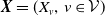
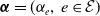
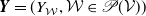
. An example of this notation is provided in Figure 1, where vertex 1 acts as the tree’s root. We refer to Section 3.3 of Saoub (Reference Saoub2021) for further insight on the terminology surrounding rooted trees.
$v \in \mathcal{V}$
. An example of this notation is provided in Figure 1, where vertex 1 acts as the tree’s root. We refer to Section 3.3 of Saoub (Reference Saoub2021) for further insight on the terminology surrounding rooted trees.
Filial relations in a rooted tree.

By encrypting a MRF on a tree, the random vector’s dependence scheme inherits the structural properties of the latter. For instance, the correlation between two of its components decays multiplicatively along the path between them. Although constraining feasible dependence schemes, this comes with the benefit of a greater interpretability: this is the idea underlying probabilistic graphical models.
The construction of tree-structured MRFs with Poisson marginal distributions relies on the binomial thinning operator, denoted by
 $\circ$
, defined in terms of a random variable Y taking values in
$\circ$
, defined in terms of a random variable Y taking values in
 $\mathbb{N}$
as
$\mathbb{N}$
as
 $\theta \circ Y \, :\!= \, \sum_{j=1}^{Y} I_{j}^{(\theta)}, \; \theta \in [0, 1],$
where
$\theta \circ Y \, :\!= \, \sum_{j=1}^{Y} I_{j}^{(\theta)}, \; \theta \in [0, 1],$
where
 $ \{I_{j}^{(\theta)}, j \in \mathbb{N}_1 \} $
is a sequence of independent Bernoulli random variables with a probability of success
$ \{I_{j}^{(\theta)}, j \in \mathbb{N}_1 \} $
is a sequence of independent Bernoulli random variables with a probability of success
 $\theta$
; see Steutel et al. (Reference Steutel, Vervaat and Wolfe1983). This operation can be interpreted as sampling among Y elements, each with probability
$\theta$
; see Steutel et al. (Reference Steutel, Vervaat and Wolfe1983). This operation can be interpreted as sampling among Y elements, each with probability
 $\theta$
of being selected independently. We refer the interested reader to Weiß (Reference Weiß2008) for further insight on the binomial thinning operator.
$\theta$
of being selected independently. We refer the interested reader to Weiß (Reference Weiß2008) for further insight on the binomial thinning operator.
2.1. Main characteristics of tree-structured MRFs with Poisson marginal distributions
To construct a risk model with heterogeneous marginal behaviors in Section 3, we define tree-structured MRFs with Poisson marginals where each component has its own mean parameter
 $\lambda_v$
,
$\lambda_v$
,
 $v \in \mathcal{V}$
.
$v \in \mathcal{V}$
.
Theorem 2.2. Consider a tree
 $ \mathcal{T} = (\mathcal{V}, \mathcal{E})$
, and let
$ \mathcal{T} = (\mathcal{V}, \mathcal{E})$
, and let
 $\mathcal{T}_r$
be its rooted version, for some
$\mathcal{T}_r$
be its rooted version, for some
 $r \in \mathcal{V}$
. Given a vector of mean parameters
$r \in \mathcal{V}$
. Given a vector of mean parameters
 $\boldsymbol{\lambda}=(\lambda_v,\,v\in\mathcal{V})$
where
$\boldsymbol{\lambda}=(\lambda_v,\,v\in\mathcal{V})$
where
 $\lambda_v\gt0$
for every
$\lambda_v\gt0$
for every
 $v\in\mathcal{V}$
and a vector of dependence parameters
$v\in\mathcal{V}$
and a vector of dependence parameters
 $\boldsymbol{\alpha} = (\alpha_e,\, e\in \mathcal{E})$
where
$\boldsymbol{\alpha} = (\alpha_e,\, e\in \mathcal{E})$
where
 $\alpha_{(\mathrm{pa}(v), v)} \in (0, \min(\sqrt{{\lambda_{v}}/{\lambda_{\mathrm{pa}(v)}}}, \sqrt{{\lambda_{\mathrm{pa}(v)}}/{\lambda_{v}}})]$
for every
$\alpha_{(\mathrm{pa}(v), v)} \in (0, \min(\sqrt{{\lambda_{v}}/{\lambda_{\mathrm{pa}(v)}}}, \sqrt{{\lambda_{\mathrm{pa}(v)}}/{\lambda_{v}}})]$
for every
 $(\mathrm{pa}(v), v)\in \mathcal{E}$
. Let
$(\mathrm{pa}(v), v)\in \mathcal{E}$
. Let
 $\boldsymbol{{L}}=(L_v,\,v\in\mathcal{V})$
be a vector of independent random variables such that
$\boldsymbol{{L}}=(L_v,\,v\in\mathcal{V})$
be a vector of independent random variables such that
 $L_v\sim \text{Poisson}(\lambda_v ( 1- \alpha_{(\mathrm{pa}(v), v)}\sqrt{\lambda_{\mathrm{pa}(v)}/\lambda_v}))$
for every
$L_v\sim \text{Poisson}(\lambda_v ( 1- \alpha_{(\mathrm{pa}(v), v)}\sqrt{\lambda_{\mathrm{pa}(v)}/\lambda_v}))$
for every
 $v\in\mathcal{V}$
, with
$v\in\mathcal{V}$
, with
 $\alpha_{(\mathrm{pa}(r), r)}=0$
since the root has no parent. Define
$\alpha_{(\mathrm{pa}(r), r)}=0$
since the root has no parent. Define
 $\boldsymbol{{N}} = (N_v,\, v \in \mathcal{V})$
as a vector of random variables such that
$\boldsymbol{{N}} = (N_v,\, v \in \mathcal{V})$
as a vector of random variables such that
 \begin{align}N_v = \begin{cases} L_r, & \text{if } v=r \\[3pt] \left(\alpha_{(\mathrm{pa}(v), v)}\sqrt{\frac{\lambda_v}{\lambda_{\mathrm{pa}(v)}}} \right)\circ N_{\mathrm{pa}(v)}+ L_v,& \text{if } v\in\mathrm{dsc}(r) \end{cases},\quad \text{for every } v\in\mathcal{V}.\end{align}
Then,
 $\boldsymbol{{N}}$
is a MRF with a unique joint distribution whichever the chosen root of
$\boldsymbol{{N}}$
is a MRF with a unique joint distribution whichever the chosen root of
 $\mathcal{T}$
, where the random variable
$\mathcal{T}$
, where the random variable
 $N_v$
follows a Poisson distribution of parameter
$N_v$
follows a Poisson distribution of parameter
 $\lambda_v$
, for all
$\lambda_v$
, for all
 $v\in \mathcal{V}$
.
$v\in \mathcal{V}$
.
Henceforth, we write
 $\boldsymbol{{N}}\sim \text{MPMRF}(\boldsymbol{\lambda}, \boldsymbol{\alpha}, \mathcal{T})$
to signify
$\boldsymbol{{N}}\sim \text{MPMRF}(\boldsymbol{\lambda}, \boldsymbol{\alpha}, \mathcal{T})$
to signify
 $\boldsymbol{{N}}$
admits the stochastic representation in (2.2), and we let
$\boldsymbol{{N}}$
admits the stochastic representation in (2.2), and we let
 ${\boldsymbol{\Lambda}}$
denote the set of admissible parameters
${\boldsymbol{\Lambda}}$
denote the set of admissible parameters
 $(\boldsymbol{\lambda}, \boldsymbol{\alpha})$
. We write
$(\boldsymbol{\lambda}, \boldsymbol{\alpha})$
. We write
 $\mathbb{MPMRF}$
the family of all such distributions for
$\mathbb{MPMRF}$
the family of all such distributions for
 $\boldsymbol{{N}}$
.
$\boldsymbol{{N}}$
.
The MRF studied in Côté et al. (Reference Côté, Cossette and Marceau2025b) is a special case of the MRF constructed in Theorem 2.2, where the mean parameters are homogeneous. In (2.2), the components of
 $\boldsymbol{{N}}$
, except the root, are defined as the sum of two independent random variables. We interpret them as the propagation and the innovation random variables, respectively. The propagation random variable
$\boldsymbol{{N}}$
, except the root, are defined as the sum of two independent random variables. We interpret them as the propagation and the innovation random variables, respectively. The propagation random variable
 $(\alpha_{(\mathrm{pa}(v), v)}\sqrt{{\lambda_v}/{\lambda_{\mathrm{pa}(v)}}} )\circ N_{\mathrm{pa}(v)}$
expresses the number of events that have duplicated by binomial thinning from
$(\alpha_{(\mathrm{pa}(v), v)}\sqrt{{\lambda_v}/{\lambda_{\mathrm{pa}(v)}}} )\circ N_{\mathrm{pa}(v)}$
expresses the number of events that have duplicated by binomial thinning from
 $N_{\mathrm{pa}(v)}$
to
$N_{\mathrm{pa}(v)}$
to
 $N_v$
. The innovation random variable
$N_v$
. The innovation random variable
 $L_v$
expresses the number of events occurring at vertex v that have not propagated from vertex
$L_v$
expresses the number of events occurring at vertex v that have not propagated from vertex
 $\mathrm{pa}(v)$
. The thinning parameter
$\mathrm{pa}(v)$
. The thinning parameter
 $\alpha_{(\mathrm{pa}(v), v)}\sqrt{{\lambda_v}/{\lambda_{\mathrm{pa}(v)}}}$
for the propagation random variable is an adjustment of the dependence parameter
$\alpha_{(\mathrm{pa}(v), v)}\sqrt{{\lambda_v}/{\lambda_{\mathrm{pa}(v)}}}$
for the propagation random variable is an adjustment of the dependence parameter
 $\alpha_{(\mathrm{pa}(v), v)}$
taking into account the heterogeneous means, so that the correlation between
$\alpha_{(\mathrm{pa}(v), v)}$
taking into account the heterogeneous means, so that the correlation between
 $N_{\mathrm{pa}(v)}$
and
$N_{\mathrm{pa}(v)}$
and
 $N_v$
is
$N_v$
is
 $\alpha_{(\mathrm{pa}(v), v)}$
. The upper bound
$\alpha_{(\mathrm{pa}(v), v)}$
. The upper bound
 $\alpha_{(\mathrm{pa}(v),v)} \lt\min(\sqrt{\lambda_v/\lambda_{\mathrm{pa}(v)}},\sqrt{\lambda_{\mathrm{pa}(v)}/\lambda_v})$
stems from the fact that dependence is characterized by this thinning mechanism. The fraction of events propagating from one random variable to another cannot exceed the root of the ratio of the marginal rates; otherwise, the innovation component would require more inherited events than the number of events possible on the parent. The admissible parameter space therefore reflects a structural feature of event-sharing mechanisms in count data. Note that any vertex can be chosen as the root of the tree; accordingly, the constraint on the dependence parameters takes into account the reversibility of parent–child relationships that may occur, thus preserving the root-free formulation of the distribution; see Remark 2.3. For illustration, if
$\alpha_{(\mathrm{pa}(v),v)} \lt\min(\sqrt{\lambda_v/\lambda_{\mathrm{pa}(v)}},\sqrt{\lambda_{\mathrm{pa}(v)}/\lambda_v})$
stems from the fact that dependence is characterized by this thinning mechanism. The fraction of events propagating from one random variable to another cannot exceed the root of the ratio of the marginal rates; otherwise, the innovation component would require more inherited events than the number of events possible on the parent. The admissible parameter space therefore reflects a structural feature of event-sharing mechanisms in count data. Note that any vertex can be chosen as the root of the tree; accordingly, the constraint on the dependence parameters takes into account the reversibility of parent–child relationships that may occur, thus preserving the root-free formulation of the distribution; see Remark 2.3. For illustration, if
 $(\lambda_1,\lambda_2) = (5,5)$
, the upper bound is 1, maximal correlation. If
$(\lambda_1,\lambda_2) = (5,5)$
, the upper bound is 1, maximal correlation. If
 $(\lambda_1,\lambda_2) = (3,5)$
, the upper bound is
$(\lambda_1,\lambda_2) = (3,5)$
, the upper bound is
 $\sqrt{0.6} \approx\!0.77$
, compared to the Fréchet upper bound of
$\sqrt{0.6} \approx\!0.77$
, compared to the Fréchet upper bound of
 $\approx\!0.97$
.
$\approx\!0.97$
.
Remark 2.3. As put forth in the proof of Theorem 2.2, the symmetry of pairwise stochastic dynamics, combined with the local Markov property, yields a root-free distribution of the MRF. The directionality seemingly implied by the necessity to choose a root is illusory: to define a parent–child dynamic is necessary to have a binomial thinning representation, but it has no impact on the joint distribution of
 $\boldsymbol{{N}}$
. The model is thus truly undirected; we will provide in Section 2.2 a root-free stochastic construction. The artificial directionality, required for the binomial thinning representation, is what allows an iterative way of proceeding along trees, resulting in algorithmic efficiency. A similar situation occurs for tree-structured Ising models; see Côté et al. (Reference Côté, Cossette and Marceau2025a).
$\boldsymbol{{N}}$
. The model is thus truly undirected; we will provide in Section 2.2 a root-free stochastic construction. The artificial directionality, required for the binomial thinning representation, is what allows an iterative way of proceeding along trees, resulting in algorithmic efficiency. A similar situation occurs for tree-structured Ising models; see Côté et al. (Reference Côté, Cossette and Marceau2025a).
Remark 2.4. Compared to the homogeneous-mean model in Côté et al. (Reference Côté, Cossette and Marceau2025b),
 $\boldsymbol{\alpha}$
is not a true dependence parameter, as it is constrained by
$\boldsymbol{\alpha}$
is not a true dependence parameter, as it is constrained by
 $\boldsymbol{\lambda}$
. To circumvent this, one could let
$\boldsymbol{\lambda}$
. To circumvent this, one could let
 $\theta_v = \alpha_{(\mathrm{pa}(v), v)}\sqrt{{\lambda_v}/{\lambda_{\mathrm{pa}(v)}}} $
, and
$\theta_v = \alpha_{(\mathrm{pa}(v), v)}\sqrt{{\lambda_v}/{\lambda_{\mathrm{pa}(v)}}} $
, and
 $\boldsymbol{\theta}$
would be a true dependence parameter, ranging from 0 to 1. The values of
$\boldsymbol{\theta}$
would be a true dependence parameter, ranging from 0 to 1. The values of
 $\boldsymbol{\theta}$
would however vary with the root, so this parameter change would come at the cost of the undirectionality of the model. Also note that, because the constraints on
$\boldsymbol{\theta}$
would however vary with the root, so this parameter change would come at the cost of the undirectionality of the model. Also note that, because the constraints on
 $\boldsymbol{\alpha}$
come directly from the binomial thinning operations, they should not be limiting if the stochastic dynamics underlying the data are effectively of propagation and innovation.
$\boldsymbol{\alpha}$
come directly from the binomial thinning operations, they should not be limiting if the stochastic dynamics underlying the data are effectively of propagation and innovation.
The following sequence of joint pgfs {
 $\eta_{v}^{\mathcal{T}_r},\,v\in\mathcal{V}\}$
will prove useful throughout the paper.
$\eta_{v}^{\mathcal{T}_r},\,v\in\mathcal{V}\}$
will prove useful throughout the paper.
Definition 2.5. Consider a tree
 $ \mathcal{T} = (\mathcal{V}, \mathcal{E})$
, and let
$ \mathcal{T} = (\mathcal{V}, \mathcal{E})$
, and let
 $\mathcal{T}_r$
be its rooted version,
$\mathcal{T}_r$
be its rooted version,
 $r \in \mathcal{V}$
. For any vector
$r \in \mathcal{V}$
. For any vector
 $\boldsymbol{\theta}$
of thinning parameters, let
$\boldsymbol{\theta}$
of thinning parameters, let
 $\boldsymbol{\theta}_{\mathrm{dsc}(v)} = (\theta_{j },\, j \in \mathrm{dsc}(v))$
for all
$\boldsymbol{\theta}_{\mathrm{dsc}(v)} = (\theta_{j },\, j \in \mathrm{dsc}(v))$
for all
 $v\in\mathcal{V}$
. We define
$v\in\mathcal{V}$
. We define
 $\{\eta_{v}^{\mathcal{T}_r},\,v\in\mathcal{V}\}$
as a sequence of joint pgfs through the recursive relation
$\{\eta_{v}^{\mathcal{T}_r},\,v\in\mathcal{V}\}$
as a sequence of joint pgfs through the recursive relation
 \begin{equation}\eta_{v}^{\mathcal{T}_r}(\boldsymbol{{t}}_{v\mathrm{dsc}(v)};\;\;\boldsymbol{\theta}_{\mathrm{dsc}(v)}) \, :\!= \, t_v \prod_{j\in\mathrm{ch}(v)} \left(1 - \theta_j+ \theta_j \eta_{j}^{\mathcal{T}_r}(\boldsymbol{{t}}_{j\mathrm{dsc}(j)};\;\;\boldsymbol{\theta}_{\mathrm{dsc}(j)}) \right)\!, \quad\boldsymbol{{t}}\in[\!-1,1]^d,\end{equation}
where
 $\boldsymbol{{t}}_{v\mathrm{dsc}(v)}$
is a short-hand notation for the vector
$\boldsymbol{{t}}_{v\mathrm{dsc}(v)}$
is a short-hand notation for the vector
 $(t_j, \, j \in \{v\} \cup \mathrm{dsc}(v))$
, and with the convention
$(t_j, \, j \in \{v\} \cup \mathrm{dsc}(v))$
, and with the convention
 $\eta_{j}^{\mathcal{T}_r}(\boldsymbol{{t}}_{j\mathrm{dsc}(j)};\;\boldsymbol{\theta}_{\mathrm{dsc}(j)}) = t_j$
for vertices j that have no children according to the rooting in r.
$\eta_{j}^{\mathcal{T}_r}(\boldsymbol{{t}}_{j\mathrm{dsc}(j)};\;\boldsymbol{\theta}_{\mathrm{dsc}(j)}) = t_j$
for vertices j that have no children according to the rooting in r.
In the following proposition, we present the joint pmf and joint pgf of
 $\boldsymbol{{N}}$
as in (2.2).
$\boldsymbol{{N}}$
as in (2.2).
Proposition 2.6. Let
 $\boldsymbol{{N}} \sim \text{MPMRF}(\boldsymbol{\lambda}, \boldsymbol{\alpha}, \mathcal{T})$
, where
$\boldsymbol{{N}} \sim \text{MPMRF}(\boldsymbol{\lambda}, \boldsymbol{\alpha}, \mathcal{T})$
, where
 $(\boldsymbol{\lambda},\boldsymbol{\alpha})\in\boldsymbol{\Lambda}$
. For a chosen root
$(\boldsymbol{\lambda},\boldsymbol{\alpha})\in\boldsymbol{\Lambda}$
. For a chosen root
 $r \in \mathcal{V}$
, let
$r \in \mathcal{V}$
, let
 $\mathcal{T}_r$
be the rooted version of
$\mathcal{T}_r$
be the rooted version of
 $\mathcal{T}$
and
$\mathcal{T}$
and
 $\zeta_{L_v} = \lambda_v ( 1- \alpha_{(\mathrm{pa}(v), v)}\sqrt{\lambda_{\mathrm{pa}(v)}/\lambda_v})$
for
$\zeta_{L_v} = \lambda_v ( 1- \alpha_{(\mathrm{pa}(v), v)}\sqrt{\lambda_{\mathrm{pa}(v)}/\lambda_v})$
for
 $v \in \mathcal{V}\backslash\{r\}$
. Then,
$v \in \mathcal{V}\backslash\{r\}$
. Then,
-
(i) the joint pmf of
 $\boldsymbol{{N}}$
is given by (2.4)for
\begin{equation}p_{\boldsymbol{{N}}}(\boldsymbol{{x}}) = \frac{\mathrm{e}^{-\lambda_r}\lambda_r^{x_r}}{x_r!} \prod_{v\in\mathrm{dsc}(r)} \sum_{k=0}^{\min(x_{\mathrm{pa}(v)},x_v)} \frac{{ \mathrm{e}}^{-\zeta_{L_v}} (\zeta_{L_v})^{x_v-k}}{(x_v-k)!} \binom{x_{\mathrm{pa}(v)}}{k} \left( \theta_v \right)^{k} \left(1- \theta_v\right)^{x_{\mathrm{pa}(v)}-k},\end{equation}
$\boldsymbol{{x}} \in \mathbb{N}^d$
, where
$\theta_v = \alpha_{(\mathrm{pa}(v),v)}\sqrt{{\lambda_v}/{\lambda_{\mathrm{pa}(v)}}}$
for all
$v\in \mathrm{dsc}(r)$
;
$\boldsymbol{{N}}$
is given by (2.4)for
\begin{equation}p_{\boldsymbol{{N}}}(\boldsymbol{{x}}) = \frac{\mathrm{e}^{-\lambda_r}\lambda_r^{x_r}}{x_r!} \prod_{v\in\mathrm{dsc}(r)} \sum_{k=0}^{\min(x_{\mathrm{pa}(v)},x_v)} \frac{{ \mathrm{e}}^{-\zeta_{L_v}} (\zeta_{L_v})^{x_v-k}}{(x_v-k)!} \binom{x_{\mathrm{pa}(v)}}{k} \left( \theta_v \right)^{k} \left(1- \theta_v\right)^{x_{\mathrm{pa}(v)}-k},\end{equation}
$\boldsymbol{{x}} \in \mathbb{N}^d$
, where
$\theta_v = \alpha_{(\mathrm{pa}(v),v)}\sqrt{{\lambda_v}/{\lambda_{\mathrm{pa}(v)}}}$
for all
$v\in \mathrm{dsc}(r)$
;
-
(ii) the joint pgf of
$\boldsymbol{{N}}$
is given by (2.5)where
\begin{equation}\mathcal{P}_{\boldsymbol{{N}}}(\boldsymbol{{t}}) = \prod_{v\in\mathcal{V}} \mathrm{e}^{\zeta_{L_v}\left(\eta_{v}^{\mathcal{T}_r}\left(\boldsymbol{{t}}_{v\mathrm{dsc}(v)};\,\boldsymbol{\theta}_{\mathrm{dsc}(v)}\right) - 1\right)},\quad \boldsymbol{{t}}\in[\!-1,1]^d,\end{equation}
$\boldsymbol{\theta}_{\mathrm{dsc}(v)}= (\alpha_{(\mathrm{pa}(k), k)}\sqrt{{\lambda_k}/{\lambda_{\mathrm{pa}(k)}}}, \, k \in \mathrm{dsc}(v))$
is the vector of thinning parameters for the propagation random variables according to a rooting in r.


The joint pmf in (2.4) factorizes along the tree, underscoring that
 $\boldsymbol{{N}}$
is a MRF. For further discussions on Gibbs distributions and pmf factorization, we refer to Appendix B, as well as Chapter 4.2 of Cressie and Wikle (Reference Cressie and Wikle2015) and Côté et al. (Reference Côté, Cossette and Marceau2025b). The analytical form of the joint pmf in (2.4) enables efficient numerical evaluation of the likelihood, making it particularly well suited for parameter estimation procedures, as shown in Sections 5 and 6.
$\boldsymbol{{N}}$
is a MRF. For further discussions on Gibbs distributions and pmf factorization, we refer to Appendix B, as well as Chapter 4.2 of Cressie and Wikle (Reference Cressie and Wikle2015) and Côté et al. (Reference Côté, Cossette and Marceau2025b). The analytical form of the joint pmf in (2.4) enables efficient numerical evaluation of the likelihood, making it particularly well suited for parameter estimation procedures, as shown in Sections 5 and 6.
In the upcoming subsection, we show that every distribution of
 $\mathbb{MPMRF}$
may be reparameterized such that
$\mathbb{MPMRF}$
may be reparameterized such that
 $\boldsymbol{{N}}$
admits an alternative stochastic representation based on common shocks. Whereas models based on the common-shock approach, whose family of distributions we write
$\boldsymbol{{N}}$
admits an alternative stochastic representation based on common shocks. Whereas models based on the common-shock approach, whose family of distributions we write
 $\mathbb{MPCS}$
, may become intractable in high dimensions due to the exponential growth in the number of possible shock configurations, the
$\mathbb{MPCS}$
, may become intractable in high dimensions due to the exponential growth in the number of possible shock configurations, the
 $\mathbb{MPMRF}$
family scales conveniently to high dimensions.
$\mathbb{MPMRF}$
family scales conveniently to high dimensions.
2.2. A subfamily of the multivariate Poisson distribution based on common shocks
Let
 ${\mathcal{V}} = \{1, 2, \ldots, d\}$
be a set of indices and let
${\mathcal{V}} = \{1, 2, \ldots, d\}$
be a set of indices and let
 $\mathscr{P}(\mathcal{V})$
be the power set of
$\mathscr{P}(\mathcal{V})$
be the power set of
 ${\mathcal{V}}$
, that is, the set of all subsets of
${\mathcal{V}}$
, that is, the set of all subsets of
 $\mathcal{V}$
, including the empty set and
$\mathcal{V}$
, including the empty set and
 $\mathcal{V}$
itself. For every
$\mathcal{V}$
itself. For every
 $v\in\mathcal{V}$
, let
$v\in\mathcal{V}$
, let
 $\mathscr{P}(\mathcal{V};\;v) = \{\mathcal{W} \in \mathscr{P}(\mathcal{V})\;:\; v\in \mathcal{W} \}$
, that is,
$\mathscr{P}(\mathcal{V};\;v) = \{\mathcal{W} \in \mathscr{P}(\mathcal{V})\;:\; v\in \mathcal{W} \}$
, that is,
 $\mathscr{P}(\mathcal{V};\;v)$
comprises the elements of
$\mathscr{P}(\mathcal{V};\;v)$
comprises the elements of
 $\mathscr{P}(\mathcal{V})$
in which v participates. Hence,
$\mathscr{P}(\mathcal{V})$
in which v participates. Hence,
 $\bigcup_{v\in\mathcal{V}} \mathscr{P}(\mathcal{V};\;v) = \mathscr{P}(\mathcal{V})$
. We define
$\bigcup_{v\in\mathcal{V}} \mathscr{P}(\mathcal{V};\;v) = \mathscr{P}(\mathcal{V})$
. We define
 $\boldsymbol{{Y}} = (Y_{\mathcal{W}}, \mathcal{W} \in\mathscr{P}(\mathcal{V}))$
as a vector of independent Poisson distributed random variables with a corresponding mean-parameter vector
$\boldsymbol{{Y}} = (Y_{\mathcal{W}}, \mathcal{W} \in\mathscr{P}(\mathcal{V}))$
as a vector of independent Poisson distributed random variables with a corresponding mean-parameter vector
 $\boldsymbol{\gamma}= (\gamma_{\mathcal{W}}, \, \mathcal{W}\in\mathscr{P}(\mathcal{V}))$
, with
$\boldsymbol{\gamma}= (\gamma_{\mathcal{W}}, \, \mathcal{W}\in\mathscr{P}(\mathcal{V}))$
, with
 $\gamma_{\mathcal{W}}\geq 0$
for every
$\gamma_{\mathcal{W}}\geq 0$
for every
 $\mathcal{W} \in \mathscr{P}(\mathcal{V})$
. We use the convention
$\mathcal{W} \in \mathscr{P}(\mathcal{V})$
. We use the convention
 $Y_{\mathcal{W}} = 0$
whenever
$Y_{\mathcal{W}} = 0$
whenever
 $\gamma_{\mathcal{W}} = 0$
. Letting
$\gamma_{\mathcal{W}} = 0$
. Letting
 $\boldsymbol{{D}} = (D_v,\,v \in \mathcal{V}) \sim \text{MPCS}(\boldsymbol{\lambda})$
, we have
$\boldsymbol{{D}} = (D_v,\,v \in \mathcal{V}) \sim \text{MPCS}(\boldsymbol{\lambda})$
, we have
 $D_v = \sum_{\mathcal{W} \in \mathscr{P}(\mathcal{V};\;v)} Y_{\mathcal{W}}, \; v \in \mathcal{V},$
where, from the closure on convolution of the Poisson distribution, each component of
$D_v = \sum_{\mathcal{W} \in \mathscr{P}(\mathcal{V};\;v)} Y_{\mathcal{W}}, \; v \in \mathcal{V},$
where, from the closure on convolution of the Poisson distribution, each component of
 $\boldsymbol{{D}}$
is Poisson distributed with parameter
$\boldsymbol{{D}}$
is Poisson distributed with parameter
 $\lambda_v = \sum_{\mathcal{W} \in \mathscr{P}(\mathcal{V};\;v)} \gamma_{\mathcal{W}}$
. The joint pgf of
$\lambda_v = \sum_{\mathcal{W} \in \mathscr{P}(\mathcal{V};\;v)} \gamma_{\mathcal{W}}$
. The joint pgf of
 $\boldsymbol{{D}}$
is given by
$\boldsymbol{{D}}$
is given by
 \begin{equation} \mathcal{P}_{\boldsymbol{{D}}}(\boldsymbol{{t}}) = \mathrm{e}^{\left({\gamma_0 + \sum_{\mathcal{W} \in \mathscr{P}(\mathcal{V})} \gamma_{\mathcal{W}} \prod_{v \in \mathcal{W}} t_{v}}\right)}, \quad \boldsymbol{{t}}\in[\!-1,1]^d, \end{equation}
with
 $\gamma_0 = - \sum_{\mathcal{W}\in \mathscr{P}(\mathcal{V})} \gamma_{\mathcal{W}}$
. We recall that the parameter vector
$\gamma_0 = - \sum_{\mathcal{W}\in \mathscr{P}(\mathcal{V})} \gamma_{\mathcal{W}}$
. We recall that the parameter vector
 $\boldsymbol{\gamma}$
is of length
$\boldsymbol{\gamma}$
is of length
 $|\mathscr{P}(\mathcal{V})| = 2^d$
. This may make computations regarding the multivariate Poisson distribution cumbersome, as discussed earlier.
$|\mathscr{P}(\mathcal{V})| = 2^d$
. This may make computations regarding the multivariate Poisson distribution cumbersome, as discussed earlier.
The following proposition provides an alternative parameterization and stochastic representation of
 $\boldsymbol{{N}}$
in terms of common shocks.
$\boldsymbol{{N}}$
in terms of common shocks.
Proposition 2.7. Consider a tree
 $\mathcal{T}= (\mathcal{V},\mathcal{E})$
and, for every
$\mathcal{T}= (\mathcal{V},\mathcal{E})$
and, for every
 $v\in\mathcal{V}$
, let
$v\in\mathcal{V}$
, let
 $\Theta_v$
be the set of all subtrees of
$\Theta_v$
be the set of all subtrees of
 $\mathcal{T}$
in which v participates, meaning
$\mathcal{T}$
in which v participates, meaning
 $\Theta_v = \{\mathcal{W} \in \mathscr{P}(\mathcal{V};\;v)$
: for every
$\Theta_v = \{\mathcal{W} \in \mathscr{P}(\mathcal{V};\;v)$
: for every
 $i, j \in \!\mathcal{W}, \, k,l \in\! \mathcal{W}$
for every
$i, j \in \!\mathcal{W}, \, k,l \in\! \mathcal{W}$
for every
 $(k, l) \in\! \mathrm{path}(i,j)\}$
. If
$(k, l) \in\! \mathrm{path}(i,j)\}$
. If
 $\boldsymbol{{N}}\sim\text{MPMRF}(\boldsymbol{\lambda}, \boldsymbol{\alpha}, \mathcal{T})$
, with
$\boldsymbol{{N}}\sim\text{MPMRF}(\boldsymbol{\lambda}, \boldsymbol{\alpha}, \mathcal{T})$
, with
 $(\boldsymbol{\lambda},\boldsymbol{\alpha})\in{\boldsymbol{\Lambda}}$
, then
$(\boldsymbol{\lambda},\boldsymbol{\alpha})\in{\boldsymbol{\Lambda}}$
, then
 $\boldsymbol{{N}}$
admits the following alternative stochastic representation:
$\boldsymbol{{N}}$
admits the following alternative stochastic representation:
 \begin{equation} N_v = \sum_{\mathcal{W}\in\Theta_v} Y_{\mathcal{W}},\quad v\in\mathcal{V}, \end{equation}
where
 $\{Y_{\mathcal{W}},\, \mathcal{W}\in\bigcup_{v\in\mathcal{V}}\Theta_v\}$
are independent Poisson random variables of respective parameters
$\{Y_{\mathcal{W}},\, \mathcal{W}\in\bigcup_{v\in\mathcal{V}}\Theta_v\}$
are independent Poisson random variables of respective parameters
 \begin{equation} \gamma_{\mathcal{W}} = \left( \prod_{w\in \mathcal{W}} \lambda_w \right)\left(\prod_{(i,j)\in\mathcal{E}_{\mathcal{W}}} \frac{\alpha_{(i,j)}}{\sqrt{\lambda_i\lambda_j}}\right)\left(\prod_{(i,j)\in\mathcal{E}^{\dagger}_{\mathcal{W}}} \left(1-\alpha_{(i,j)}\sqrt{\frac{\lambda_j}{\lambda_i}}\right)\right)\!, \quad \mathcal{W}\in \bigcup_{v\in\mathcal{V}}\Theta_v, \end{equation}
with
 $\mathcal{E}_{\mathcal{W}} = \{(i,j)\in\mathcal{E} :\, i,j\in \mathcal{W}\}$
and
$\mathcal{E}_{\mathcal{W}} = \{(i,j)\in\mathcal{E} :\, i,j\in \mathcal{W}\}$
and
 $\mathcal{E}_{\mathcal{W}}^{\dagger} = \{(i,j)\in\mathcal{E} :\, i\in \mathcal{W}, j\not\in \mathcal{W}\}$
.
$\mathcal{E}_{\mathcal{W}}^{\dagger} = \{(i,j)\in\mathcal{E} :\, i\in \mathcal{W}, j\not\in \mathcal{W}\}$
.
The upper limit for
 $\alpha_e$
,
$\alpha_e$
,
 $e\in\mathcal{E}$
, for
$e\in\mathcal{E}$
, for
 $(\boldsymbol{\lambda},\boldsymbol{\alpha})$
to be in
$(\boldsymbol{\lambda},\boldsymbol{\alpha})$
to be in
 ${\boldsymbol{\Lambda}}$
, ensures
${\boldsymbol{\Lambda}}$
, ensures
 $\gamma_{\mathcal{W}}\geq0$
for every
$\gamma_{\mathcal{W}}\geq0$
for every
 $\mathcal{W}\in\bigcup_{v\in\mathcal{V}}\Theta_v$
.
$\mathcal{W}\in\bigcup_{v\in\mathcal{V}}\Theta_v$
.
Given Proposition 2.7, one easily sees that
 $\boldsymbol{{N}}$
follows a multivariate Poisson with vector of parameters
$\boldsymbol{{N}}$
follows a multivariate Poisson with vector of parameters
 $\boldsymbol{\gamma}= (\gamma_V, \, V\in\mathscr{P}(\mathcal{V}))$
such that
$\boldsymbol{\gamma}= (\gamma_V, \, V\in\mathscr{P}(\mathcal{V}))$
such that
 \begin{equation*} \gamma_{V} =\begin{cases}\gamma_{\mathcal{W}},&\text{if }{\mathcal{W}\in{\bigcup_{v \in \mathcal{V}}\Theta_v}}\\[3pt]0,&\text{else}\end{cases},\quad V \in \mathscr{P}(\mathcal{V}).\end{equation*}
Hence, Proposition 2.7 shows
 $\mathbb{MPMRF}\subseteq\mathbb{MPCS}$
. For a further discussion on the connection between the thinning and the common-shock approaches for Poisson random variables, see Liu et al. (Reference Liu, Shi, Yao and Yang2024) and their Remark 2.3 in particular. Although the number of non-zero parameters in the common-shock representation of
$\mathbb{MPMRF}\subseteq\mathbb{MPCS}$
. For a further discussion on the connection between the thinning and the common-shock approaches for Poisson random variables, see Liu et al. (Reference Liu, Shi, Yao and Yang2024) and their Remark 2.3 in particular. Although the number of non-zero parameters in the common-shock representation of
 $\mathbb{MPMRF}$
is lower than
$\mathbb{MPMRF}$
is lower than
 $2^d$
(as for
$2^d$
(as for
 $\mathbb{MPCS}$
), the reduction is not substantial enough to overcome computation challenges. Moreover, the parameterization in terms of
$\mathbb{MPCS}$
), the reduction is not substantial enough to overcome computation challenges. Moreover, the parameterization in terms of
 $\boldsymbol{\gamma}$
intertwines the dependencies and the marginals, thereby removing their intended parametric disconnection. Theorem 2.2 remains a simpler representation, as put forth in Example 2.8. The family
$\boldsymbol{\gamma}$
intertwines the dependencies and the marginals, thereby removing their intended parametric disconnection. Theorem 2.2 remains a simpler representation, as put forth in Example 2.8. The family
 $\mathbb{MPMRF}$
being a subset of
$\mathbb{MPMRF}$
being a subset of
 $\mathbb{MPCS}$
, it cannot grow out of the latters’ limitations in terms of achievable dependence structures. The advantage of
$\mathbb{MPCS}$
, it cannot grow out of the latters’ limitations in terms of achievable dependence structures. The advantage of
 $\mathbb{MPMRF}$
over generic elements of
$\mathbb{MPMRF}$
over generic elements of
 $\mathbb{MPCS}$
comes from its binomial thinning stochastic representation (2.2) and the computational efficiency ensuing.
$\mathbb{MPCS}$
comes from its binomial thinning stochastic representation (2.2) and the computational efficiency ensuing.
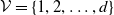
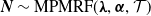
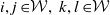
Example 2.8. A 5-variate distribution in
 $\mathbb{MPCS}$
generally requires
$\mathbb{MPCS}$
generally requires
 $2^5 = 32$
parameters. Consider
$2^5 = 32$
parameters. Consider
 $\boldsymbol{{N}} \sim \text{MPMRF}(\boldsymbol{\lambda}, \boldsymbol{\alpha}, \mathcal{T})$
where
$\boldsymbol{{N}} \sim \text{MPMRF}(\boldsymbol{\lambda}, \boldsymbol{\alpha}, \mathcal{T})$
where
 $\mathcal{T}$
is structured as in Figure 2. Using (2.7), we develop
$\mathcal{T}$
is structured as in Figure 2. Using (2.7), we develop
 $\boldsymbol{{N}}$
into its common shock representation in Figure 2. One notices that constructing
$\boldsymbol{{N}}$
into its common shock representation in Figure 2. One notices that constructing
 $\boldsymbol{\gamma}$
demands
$\boldsymbol{\gamma}$
demands
 $|\bigcup_{v \in \mathcal{V}}\Theta_v| = 17$
non-zero parameters, which is a meaningful diminution, but still much higher than the nine parameters required by the representation in Theorem 2.2. A comparison of
$|\bigcup_{v \in \mathcal{V}}\Theta_v| = 17$
non-zero parameters, which is a meaningful diminution, but still much higher than the nine parameters required by the representation in Theorem 2.2. A comparison of
 $N_1$
and
$N_1$
and
 $N_2$
in Figure 2 reveals that a change in
$N_2$
in Figure 2 reveals that a change in
 $\gamma_{\{1,2\}}$
affects both mean parameters of the random variables
$\gamma_{\{1,2\}}$
affects both mean parameters of the random variables
 $N_1$
and
$N_1$
and
 $N_2$
. The parameters
$N_2$
. The parameters
 $\gamma_{\mathcal{W}}$
associated with each
$\gamma_{\mathcal{W}}$
associated with each
 $Y_{\mathcal{W}}$
in Figure 2.8 are given in Table 1. We verify easily that
$Y_{\mathcal{W}}$
in Figure 2.8 are given in Table 1. We verify easily that
 $N_v\sim\text{Poisson}(\lambda_v)$
for every
$N_v\sim\text{Poisson}(\lambda_v)$
for every
 $v\in\{1,\ldots,5\}$
. In Table 1 of Supplement A, a numerical instance illustrates the equivalence between
$v\in\{1,\ldots,5\}$
. In Table 1 of Supplement A, a numerical instance illustrates the equivalence between
 $\mathbb{MRMRF}$
and
$\mathbb{MRMRF}$
and
 $\mathbb{MPCS}$
.
$\mathbb{MPCS}$
.
Tree
 $\mathcal{T}$
of Example 2.8 and
$\mathcal{T}$
of Example 2.8 and
 $\boldsymbol{{N}}$
components’ common shock representations.
$\boldsymbol{{N}}$
components’ common shock representations.

Proposition 2.7 makes clear the difference between
 $\mathbb{MPMRF}$
and the tree-structured multivariate Poisson distribution examined in Kızıldemir and Privault (Reference Kzldemir and Privault2017). In the latter, there are only random variables
$\mathbb{MPMRF}$
and the tree-structured multivariate Poisson distribution examined in Kızıldemir and Privault (Reference Kzldemir and Privault2017). In the latter, there are only random variables
 $Y_{\mathcal{W}}$
from the representation in (2.7) for
$Y_{\mathcal{W}}$
from the representation in (2.7) for
 $\mathcal{W}\in\mathscr{P}(\mathcal{V};\;v)$
comprising two elements, given by the set of edges
$\mathcal{W}\in\mathscr{P}(\mathcal{V};\;v)$
comprising two elements, given by the set of edges
 $\mathcal{E}$
of the graph. There are no shock random variables
$\mathcal{E}$
of the graph. There are no shock random variables
 $Y_{\mathcal{W}}$
for
$Y_{\mathcal{W}}$
for
 $|\mathcal{W}|\geq 3$
. As a consequence, the multivariate distribution does not exhibit the conditional independence relations from Definition 2.1 to render a MRF.
$|\mathcal{W}|\geq 3$
. As a consequence, the multivariate distribution does not exhibit the conditional independence relations from Definition 2.1 to render a MRF.
While previous work has extended the multivariate Poisson distribution based on common shocks to higher dimensions, no method combines minimal parameters with the wide variety of dependence structures achievable by
 $\mathbb{MPMRF}$
. For instance, Schulz et al. (Reference Schulz, Genest and Mesfioui2021) generalize the bivariate Poisson model from Genest et al. (Reference Genest, Mesfioui and Schulz2018) to higher dimensions, requiring only
$\mathbb{MPMRF}$
. For instance, Schulz et al. (Reference Schulz, Genest and Mesfioui2021) generalize the bivariate Poisson model from Genest et al. (Reference Genest, Mesfioui and Schulz2018) to higher dimensions, requiring only
 $d+1$
parameters, but this approach imposes limitations on the correlation structure by restricting dependence to a single parameter. Murphy and Schulz (Reference Murphy and Schulz2025) address this limitation with the multivariate Poisson distribution based on triangular comonotonic shocks but requires
$d+1$
parameters, but this approach imposes limitations on the correlation structure by restricting dependence to a single parameter. Murphy and Schulz (Reference Murphy and Schulz2025) address this limitation with the multivariate Poisson distribution based on triangular comonotonic shocks but requires
 $d+d(d-1)/2 = \mathcal{O}(d^2)$
parameters, still computationally intensive in high-dimensional settings. The
$d+d(d-1)/2 = \mathcal{O}(d^2)$
parameters, still computationally intensive in high-dimensional settings. The
 $\mathbb{MPMRF}$
family, by comparison, achieves complex dependence structures with only
$\mathbb{MPMRF}$
family, by comparison, achieves complex dependence structures with only
 $2d-1$
parameters, scaling more efficiently at
$2d-1$
parameters, scaling more efficiently at
 $\mathcal{O}(d)$
. This allows for convenient estimation in higher dimensions; further discussion is provided in Section 6. The comonotonic shock approach in the above papers accommodates a broader range of correlations, but it cannot be expressed as a thinning operation. One could modify
$\mathcal{O}(d)$
. This allows for convenient estimation in higher dimensions; further discussion is provided in Section 6. The comonotonic shock approach in the above papers accommodates a broader range of correlations, but it cannot be expressed as a thinning operation. One could modify
 $\mathbb{MPMRF}$
by letting the construction in (2.7) be in terms of comonotonic shocks but would therefore be unable to reexpress it in terms of an iterative stochastic construction as in (2.2). The latter is what enables efficient computational methods, as we discuss in the upcoming sections.
$\mathbb{MPMRF}$
by letting the construction in (2.7) be in terms of comonotonic shocks but would therefore be unable to reexpress it in terms of an iterative stochastic construction as in (2.2). The latter is what enables efficient computational methods, as we discuss in the upcoming sections.
3. Aggregate analysis of the portfolio
A risk model
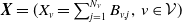 $\boldsymbol{{X}} = (X_v =\sum_{j=1}^{N_v} B_{v,j}, \; v\in\mathcal{V})$
as defined in (1.1) with
$\boldsymbol{{X}} = (X_v =\sum_{j=1}^{N_v} B_{v,j}, \; v\in\mathcal{V})$
as defined in (1.1) with
 $\boldsymbol{{N}}$
from Theorem 2.2 benefits from analytical and computable expressions, even if the dimension
$\boldsymbol{{N}}$
from Theorem 2.2 benefits from analytical and computable expressions, even if the dimension
 $d =|\mathcal{V}|$
is high. The flexibility in choosing parameters
$d =|\mathcal{V}|$
is high. The flexibility in choosing parameters
 $(\boldsymbol{\lambda},\boldsymbol{\alpha})\in\boldsymbol{\Lambda}$
and the underlying tree
$(\boldsymbol{\lambda},\boldsymbol{\alpha})\in\boldsymbol{\Lambda}$
and the underlying tree
 $\mathcal{T}$
provides a diversity of dependence structures.
$\mathcal{T}$
provides a diversity of dependence structures.
The joint Laplace–Stieltjes transform (LST) of
 $\boldsymbol{{X}}$
, denoted
$\boldsymbol{{X}}$
, denoted
 $\mathcal{L}_{\boldsymbol{{X}}}$
, used to obtain the distribution of the aggregate claim amount for the portfolio, is given by
$\mathcal{L}_{\boldsymbol{{X}}}$
, used to obtain the distribution of the aggregate claim amount for the portfolio, is given by
 \begin{equation}\mathcal{L}_{\boldsymbol{{X}}}(\boldsymbol{{t}}) =\mathbb{E}\left[\prod_{v \in \mathcal{V}} \mathrm{e}^{-t_v X_v} \right] =\mathcal{P}_{\boldsymbol{{N}}}(\mathcal{L}_{B_1}(t_1), \ldots, \mathcal{L}_{B_d}(t_d)) = \prod_{v\in\mathcal{V}} \mathrm{e}^{\zeta_{L_v}\left(\eta_{v}^{\mathcal{T}_r}(\pmb{\mathcal{L}}_{B_v}(\boldsymbol{{t}}_{v\mathrm{dsc}(v)}); \boldsymbol{\theta}_{\mathrm{dsc}(v)}) - 1\right)},\end{equation}
for
 $\boldsymbol{{t}} \in \mathbb{R}_+^d$
, with the sequence of joint pgfs
$\boldsymbol{{t}} \in \mathbb{R}_+^d$
, with the sequence of joint pgfs
 $\{\eta_{v}^{\mathcal{T}_r},\,v\in\mathcal{V}\}$
defined by the recursive relation in (2.3), and with the vectors
$\{\eta_{v}^{\mathcal{T}_r},\,v\in\mathcal{V}\}$
defined by the recursive relation in (2.3), and with the vectors
 $\pmb{\mathcal{L}}_{B_v}(\boldsymbol{{t}}_{v\mathrm{dsc}(v)}) = (\mathcal{L}_{B_{j}}(t_j), j \in \{v\} \cup \mathrm{dsc}(v))$
and
$\pmb{\mathcal{L}}_{B_v}(\boldsymbol{{t}}_{v\mathrm{dsc}(v)}) = (\mathcal{L}_{B_{j}}(t_j), j \in \{v\} \cup \mathrm{dsc}(v))$
and
 $\boldsymbol{\theta}_{\mathrm{dsc}(v)}= (\alpha_{(\mathrm{pa}(k), k)}\sqrt{{\lambda_k}/{\lambda_{\mathrm{pa}(k)}}}, k \in \mathrm{dsc}(v))$
for every
$\boldsymbol{\theta}_{\mathrm{dsc}(v)}= (\alpha_{(\mathrm{pa}(k), k)}\sqrt{{\lambda_k}/{\lambda_{\mathrm{pa}(k)}}}, k \in \mathrm{dsc}(v))$
for every
 $v\in\mathcal{V}$
.
$v\in\mathcal{V}$
.
Given
 $\mathcal{L}_{S}(t) = \mathcal{L}_{\boldsymbol{{X}}}(t,\ldots,t) = \mathcal{P}_{\boldsymbol{{N}}}(\mathcal{L}_{B_{1}}(t), \ldots, \mathcal{L}_{B_{d}}(t))$
,
$\mathcal{L}_{S}(t) = \mathcal{L}_{\boldsymbol{{X}}}(t,\ldots,t) = \mathcal{P}_{\boldsymbol{{N}}}(\mathcal{L}_{B_{1}}(t), \ldots, \mathcal{L}_{B_{d}}(t))$
,
 $t \geq 0$
(Theorem 1 of Wang, Reference Wang1998), the joint LST in (3.1) leads to the following LST of the aggregate claim S:
$t \geq 0$
(Theorem 1 of Wang, Reference Wang1998), the joint LST in (3.1) leads to the following LST of the aggregate claim S:
 \begin{equation}\mathcal{L}_S(t)= \mathrm{e}^{ \sum_{v \in \mathcal{V}} \zeta_{L_v} \left( \sum_{v \in \mathcal{V}} \frac{\zeta_{L_v}}{ \sum_{v \in \mathcal{V}} \zeta_{L_v}} \eta_v^{\mathcal{T}_r} (\pmb{\mathcal{L}}_{B_v}(t \, \boldsymbol{1}_{v\mathrm{dsc}(v)}); \boldsymbol{\theta}_{\mathrm{dsc}(v)}) - 1 \right)} = \mathrm{e}^{\lambda_S (\mathcal{L}_{C_S}(t) - 1)}, \quad t \geq 0,\end{equation}
implying that S follows a compound Poisson distribution with primary mean parameter
 $\lambda_S = \sum_{v \in \mathcal{V}} \zeta_{L_v}$
and secondary LST given by
$\lambda_S = \sum_{v \in \mathcal{V}} \zeta_{L_v}$
and secondary LST given by
 $\mathcal{L}_{C_S}(t) = \sum_{v \in \mathcal{V}}\left({\zeta_{L_v}}/{\lambda_S}\right) \eta_v^{\mathcal{T}_r} (\pmb{\mathcal{L}}_{B_v}(t \,\boldsymbol{1}_{v\mathrm{dsc}(v)}); \boldsymbol{\theta}_{\mathrm{dsc}(v)})$
,
$\mathcal{L}_{C_S}(t) = \sum_{v \in \mathcal{V}}\left({\zeta_{L_v}}/{\lambda_S}\right) \eta_v^{\mathcal{T}_r} (\pmb{\mathcal{L}}_{B_v}(t \,\boldsymbol{1}_{v\mathrm{dsc}(v)}); \boldsymbol{\theta}_{\mathrm{dsc}(v)})$
,
 $t\geq 0$
.
$t\geq 0$
.
Generating realizations of
 $\boldsymbol{{X}}$
is straightforward, given that, the stochastic representation of
$\boldsymbol{{X}}$
is straightforward, given that, the stochastic representation of
 $\boldsymbol{{N}}$
allows for an easily scalable sampling method. One generates realizations for each component of
$\boldsymbol{{N}}$
allows for an easily scalable sampling method. One generates realizations for each component of
 $\boldsymbol{{N}}$
successively; this is well suited for high-dimensional contexts. In this vein, by adapting Algorithm 2 from Côté et al. (Reference Côté, Cossette and Marceau2025b) to accommodate flexible mean parameters, one can efficiently produce a realization of
$\boldsymbol{{N}}$
successively; this is well suited for high-dimensional contexts. In this vein, by adapting Algorithm 2 from Côté et al. (Reference Côté, Cossette and Marceau2025b) to accommodate flexible mean parameters, one can efficiently produce a realization of
 $\boldsymbol{{X}}$
by independently producing a realization of
$\boldsymbol{{X}}$
by independently producing a realization of
 $\boldsymbol{{N}}$
and of the claim amounts.
$\boldsymbol{{N}}$
and of the claim amounts.
For discrete claim amount random variables, values of the pmf of S can directly be computed using the fast Fourier transform (FFT) algorithm or Panjer’s recursion. Algorithm 1 in Supplement B illustrates a procedure for our context using FFT. Discretization methods or mixed Erlang approximations may be used for continuous claim amounts. Mixed Erlang distributions are known to approximate any continuous positive distribution effectively; see for instance, Tijms (Reference Tijms1994).
Remark 3.1. Let
 $\boldsymbol{{X}}$
be a multivariate compound Poisson with
$\boldsymbol{{X}}$
be a multivariate compound Poisson with
 $\boldsymbol{{N}} \sim \text{MPMRF}(\boldsymbol{\lambda}, \boldsymbol{\alpha}, \mathcal{T})$
. We assume each
$\boldsymbol{{N}} \sim \text{MPMRF}(\boldsymbol{\lambda}, \boldsymbol{\alpha}, \mathcal{T})$
. We assume each
 ${B_v},\,v \in \mathcal{V}$
, follows a mixed Erlang distribution with parameters
${B_v},\,v \in \mathcal{V}$
, follows a mixed Erlang distribution with parameters
 $(\boldsymbol{\pi}_v, \beta_v)$
where
$(\boldsymbol{\pi}_v, \beta_v)$
where
 $\boldsymbol{\pi}_v = (\pi_{v,k}, k \in \mathbb{N}_1)$
is a vector of non-negative weight parameters,
$\boldsymbol{\pi}_v = (\pi_{v,k}, k \in \mathbb{N}_1)$
is a vector of non-negative weight parameters,
 $\sum_{k=1}^{\infty} \pi_{v,k} = 1$
, and
$\sum_{k=1}^{\infty} \pi_{v,k} = 1$
, and
 $\beta_v \gt 0$
. The LST of S in (3.2) becomes
$\beta_v \gt 0$
. The LST of S in (3.2) becomes
 \begin{equation}\mathcal{L}_{S}(t) = \exp\left\{\lambda_S \left( \sum_{v \in \mathcal{V}} \frac{\zeta_{L_v}}{ \lambda_S} \mathcal{P}_{\boldsymbol{{G}}^{\mathcal{T}_r}_v}\left\{ \left(\mathcal{P}_{\widetilde{K}_j}(\mathcal{L}_{B_{\max}}(t)),\, j\in \{v\}\cup\mathrm{dsc}(v) \right) \right\} \right) \right\} = \mathcal{P}_W(\mathcal{L}_{B_{\max}}(t)),\end{equation}
for
 $t \geq 0$
, where
$t \geq 0$
, where
 $\widetilde{K}_j$
is as defined in Appendix A.4,
$\widetilde{K}_j$
is as defined in Appendix A.4,
 $B_{\max}\sim$
Exp
$B_{\max}\sim$
Exp
 $({\max}_{v\in\mathcal{V}} \beta_{v})$
and
$({\max}_{v\in\mathcal{V}} \beta_{v})$
and
 $\boldsymbol{{G}}^{\mathcal{T}_r}_v = (G^{\mathcal{T}_r}_{v,j}, j \in \{v\} \cup \mathrm{dsc}(v))$
is a vector of discrete random variables whose joint pgf is given by
$\boldsymbol{{G}}^{\mathcal{T}_r}_v = (G^{\mathcal{T}_r}_{v,j}, j \in \{v\} \cup \mathrm{dsc}(v))$
is a vector of discrete random variables whose joint pgf is given by
 $\eta^{\mathcal{T}_r}_v(\boldsymbol{{t}}_{v\mathrm{dsc}(v)};\;\boldsymbol{\theta}_{\mathrm{dsc}(v)})$
,
$\eta^{\mathcal{T}_r}_v(\boldsymbol{{t}}_{v\mathrm{dsc}(v)};\;\boldsymbol{\theta}_{\mathrm{dsc}(v)})$
,
 $\boldsymbol{{t}}\in[\!-1,1]^d$
, as in Definition 2.5. We recognize in (3.3) the LST of a mixed Erlang distribution.
$\boldsymbol{{t}}\in[\!-1,1]^d$
, as in Definition 2.5. We recognize in (3.3) the LST of a mixed Erlang distribution.
Hence, to perform computations regarding S, one must simply compute the pmf of W, relying on (3.3) and Algorithm 1. This is at the core of Algorithm 2 in Supplement B, which computes the cumulative distribution function (cdf) of S under mixed Erlang claim amounts. With the distribution of S, one may compute the portfolio’s required capital through different risk measures. This allows to complete our first risk management task regarding the quantification of the portfolio’s risk.
4. Risk sharing
A subsequent risk management task involves the proper allocation of the portfolio’s required capital to each component. This allocation can be performed ex ante; the allocation rule divides the overall portfolio’s risk, quantified by a risk measure, into shares for each component of
 $\boldsymbol{{X}}$
based on their respective levels of risk. When dealing with positively homogeneous risk measures, Euler’s principle can be utilized to determine the value of these shares. A well-known example of such risk measures is the TVaR. For a random variable Z, the TVaR at confidence level
$\boldsymbol{{X}}$
based on their respective levels of risk. When dealing with positively homogeneous risk measures, Euler’s principle can be utilized to determine the value of these shares. A well-known example of such risk measures is the TVaR. For a random variable Z, the TVaR at confidence level
 $\kappa\in[0,1)$
is given by
$\kappa\in[0,1)$
is given by
 $ \mathrm{TVaR}_{\kappa}(Z) = \frac{1}{1 - \kappa} \int_{\kappa}^1 \text{VaR}_u(Z) \, \mathrm{d}u$
, where
$ \mathrm{TVaR}_{\kappa}(Z) = \frac{1}{1 - \kappa} \int_{\kappa}^1 \text{VaR}_u(Z) \, \mathrm{d}u$
, where
 $\mathrm{VaR}_u(Z) = \inf\{x\in\mathbb{R} \;:\; F_Z(x)\geq u\}$
, and
$\mathrm{VaR}_u(Z) = \inf\{x\in\mathbb{R} \;:\; F_Z(x)\geq u\}$
, and
 $u\in[0,1)$
. Let us recall that mixed Erlang distributions may approximate any continuous claim amount distributions; we showed in Section 3 that the pmf of S can be exactly computed in this case. The results from Cossette et al. (Reference Cossette, Mailhot and Marceau2012) are thus readily applicable for computing the exact contribution to the TVaR based on Euler’s rule. If claim amount distributions are discrete, additional manipulations are required to allocate risk. In such a case, the contribution of
$u\in[0,1)$
. Let us recall that mixed Erlang distributions may approximate any continuous claim amount distributions; we showed in Section 3 that the pmf of S can be exactly computed in this case. The results from Cossette et al. (Reference Cossette, Mailhot and Marceau2012) are thus readily applicable for computing the exact contribution to the TVaR based on Euler’s rule. If claim amount distributions are discrete, additional manipulations are required to allocate risk. In such a case, the contribution of
 $X_v$
,
$X_v$
,
 $v\in\mathcal{V}$
, to the TVaR of S under Euler’s principle is given by
$v\in\mathcal{V}$
, to the TVaR of S under Euler’s principle is given by
 \begin{align} \mathcal{C}^{\mathrm{TVaR}}_{\kappa}(X_v;\, S) &= \frac{1}{1-\kappa}\left( \mathbb{E}[X_v\unicode{x1D7D9}_{\{S\gt\mathrm{VaR}_{\kappa}(S)\}}] + \mathbb{E}[X_v|S=\mathrm{VaR}_{\kappa}(S)](F_S(\mathrm{VaR}_{\kappa}(S))-\kappa)\right) \notag\\[3pt] &= \frac{1}{1-\kappa}\left( \mathbb{E}[X_v] - \sum_{k=0}^{\mathrm{VaR}_{\kappa}(S)}\mathbb{E}[X_v\unicode{x1D7D9}_{\{S=k\}}] + \frac{F_S(\mathrm{VaR}_{\kappa}(S))-\kappa}{p_S(\mathrm{VaR}_{\kappa}(S))} \mathbb{E}[X_v\unicode{x1D7D9}_{\{S=\mathrm{VaR}_{\kappa}(S)\}}]\right)\!,\end{align}
for
 $\kappa \in [0,1)$
; see, for instance, Section 2 in Mausser and Romanko (Reference Mausser and Romanko2018).
$\kappa \in [0,1)$
; see, for instance, Section 2 in Mausser and Romanko (Reference Mausser and Romanko2018).
A risk modeler may prefer the covariance-based allocation rule instead of
 $C^{\mathrm{TVaR}}_\kappa(X_v, S)$
for
$C^{\mathrm{TVaR}}_\kappa(X_v, S)$
for
 $v \in \mathcal{V}$
. The contribution amount of risk
$v \in \mathcal{V}$
. The contribution amount of risk
 $X_v$
, denoted by
$X_v$
, denoted by
 $C^{\mathrm{Cov}}_\kappa(X_v, S)$
, is given by
$C^{\mathrm{Cov}}_\kappa(X_v, S)$
, is given by
 \begin{equation*}C^{\mathrm{Cov}}_\kappa(X_v, S) = \mathbb{E}[X_v] + \frac{\mathrm{Cov}(X_v, S)}{\mathrm{Var}(S)} \left( \mathrm{TVaR}_\kappa(S) - \mathbb{E}[S] \right)\!, \quad v \in \mathcal{V}.\end{equation*}
Both allocation rules ensure that the sum of the contributions equals
 $\mathrm{TVaR}_\kappa(S)$
, the required capital for the tail risk of the portfolio. Moreover, both rules satisfy Euler’s principle. For detailed discussions on these allocation principles, we refer the reader to Tasche (Reference Tasche1999) and McNeil et al. (Reference McNeil, Frey and Embrechts2015) and to Hesselager and Andersson (Reference Hesselager and Andersson2002) for further information on the covariance-based allocation rule.
$\mathrm{TVaR}_\kappa(S)$
, the required capital for the tail risk of the portfolio. Moreover, both rules satisfy Euler’s principle. For detailed discussions on these allocation principles, we refer the reader to Tasche (Reference Tasche1999) and McNeil et al. (Reference McNeil, Frey and Embrechts2015) and to Hesselager and Andersson (Reference Hesselager and Andersson2002) for further information on the covariance-based allocation rule.
To allocate the aggregate risk ex post, one may choose a fair risk sharing rule. A risk sharing rule is a mapping that assigns to each participant a contribution
 $h_{v,d}(S)$
such that
$h_{v,d}(S)$
such that
 $\sum_{v=1}^d h_{v,d}(S) = S$
. A rule is said to be fair if it also satisfies
$\sum_{v=1}^d h_{v,d}(S) = S$
. A rule is said to be fair if it also satisfies
 $\mathbb{E}[h_{v,d}(S)] = \mathbb{E}[X_v] = \mu_v$
for all v, ensuring participants pay their expected loss on average. In the context of peer-to-peer insurance, for instance, risk sharing rules serve to determine each participant’s contribution to the pool (Denuit et al. Reference Denuit, Dhaene and Robert2022).
$\mathbb{E}[h_{v,d}(S)] = \mathbb{E}[X_v] = \mu_v$
for all v, ensuring participants pay their expected loss on average. In the context of peer-to-peer insurance, for instance, risk sharing rules serve to determine each participant’s contribution to the pool (Denuit et al. Reference Denuit, Dhaene and Robert2022).
Linear fair rules take the form
 $h_{v,d}^{\text{lin}}(S) = \mu_v + a_{v,d}(S - \mathbb{E}[S])$
, where the coefficients
$h_{v,d}^{\text{lin}}(S) = \mu_v + a_{v,d}(S - \mathbb{E}[S])$
, where the coefficients
 $a_{v,d}$
satisfy
$a_{v,d}$
satisfy
 $\sum_{v \in \mathcal{V}} a_{v,d} = 1$
. Two notable examples include the proportional rule, where
$\sum_{v \in \mathcal{V}} a_{v,d} = 1$
. Two notable examples include the proportional rule, where
 $a_{v,d} = \mu_v / \mathbb{E}[S]$
, allocating risk in proportion to expected losses; the linear regression rule, where
$a_{v,d} = \mu_v / \mathbb{E}[S]$
, allocating risk in proportion to expected losses; the linear regression rule, where
 $a_{v,d} = \mathrm{Cov}(X_v,S)/\mathrm{Var}(S)$
, allocating deviations according to volatility. This rule minimizes the mean squared error
$a_{v,d} = \mathrm{Cov}(X_v,S)/\mathrm{Var}(S)$
, allocating deviations according to volatility. This rule minimizes the mean squared error
 $\mathbb{E}[(X_v - h_{v,d}(S))^2]$
among all linear fair rules.
$\mathbb{E}[(X_v - h_{v,d}(S))^2]$
among all linear fair rules.
The (nonlinear) conditional-mean risk sharing rule (Denuit and Dhaene, Reference Denuit and Dhaene2012), defined by
 $h_{v,d}^{\star}(S) = \mathbb{E}[X_v|S]$
, minimizes
$h_{v,d}^{\star}(S) = \mathbb{E}[X_v|S]$
, minimizes
 $\mathbb{E}[(X_v - h_{v,d}(S))^2]$
over all measurable functions
$\mathbb{E}[(X_v - h_{v,d}(S))^2]$
over all measurable functions
 $h_{v,d}$
with finite variance. This rule is Pareto-optimal under risk aversion and does not rely on individual preference inclusion, making it particularly suitable for peer-to-peer insurance frameworks (Denuit and Dhaene, Reference Denuit and Dhaene2012). For discrete distributions, we have
$h_{v,d}$
with finite variance. This rule is Pareto-optimal under risk aversion and does not rely on individual preference inclusion, making it particularly suitable for peer-to-peer insurance frameworks (Denuit and Dhaene, Reference Denuit and Dhaene2012). For discrete distributions, we have
 $\mathbb{E}[X_v|S=k] = {\mathbb{E}[X_v\unicode{x1D7D9}_{\{S=k\}}]}/{p_{S}(k)}, \; v\in\mathcal{V}, \; k\in\mathrm{supp}(S)$
.
$\mathbb{E}[X_v|S=k] = {\mathbb{E}[X_v\unicode{x1D7D9}_{\{S=k\}}]}/{p_{S}(k)}, \; v\in\mathcal{V}, \; k\in\mathrm{supp}(S)$
.
4.1. Computation of risk allocations
A crucial component for calculating both
 $\mathcal{C}^{\mathrm{TVaR}}_{\kappa}(X_v;\;S)$
and
$\mathcal{C}^{\mathrm{TVaR}}_{\kappa}(X_v;\;S)$
and
 $\mathbb{E}[X_v|S=k]$
is the expected allocation:
$\mathbb{E}[X_v|S=k]$
is the expected allocation:
 $\mathbb{E}[X_v\unicode{x1D7D9}_{\{S=k\}}]$
, for
$\mathbb{E}[X_v\unicode{x1D7D9}_{\{S=k\}}]$
, for
 $k\in\mathrm{supp}(S)$
. The significance of expected allocations in the context of capital allocation is thoroughly discussed in Blier-Wong et al. (Reference Blier-Wong, Cossette and Marceau2025). The authors introduce an ordinary generating function for expected allocations, which is defined as follows.
$k\in\mathrm{supp}(S)$
. The significance of expected allocations in the context of capital allocation is thoroughly discussed in Blier-Wong et al. (Reference Blier-Wong, Cossette and Marceau2025). The authors introduce an ordinary generating function for expected allocations, which is defined as follows.
Definition 4.1 (OGFEA). Consider a vector of discrete random variables
 $\boldsymbol{{Z}}=(Z_1,\ldots, Z_d)$
taking values in
$\boldsymbol{{Z}}=(Z_1,\ldots, Z_d)$
taking values in
 $\mathbb{N}^{d}$
. The ordinary generating function of expected allocations (OGFEA) of
$\mathbb{N}^{d}$
. The ordinary generating function of expected allocations (OGFEA) of
 $Z_v$
,
$Z_v$
,
 $v\in\{1,\ldots,d\}$
, to the sum of components
$v\in\{1,\ldots,d\}$
, to the sum of components
 $\sum_{v=1}^d Z_v$
is given by
$\sum_{v=1}^d Z_v$
is given by
 $\mathcal{P}^{[v]}_{\sum_{v=1}^d Z_v}(t) = \sum_{k=0}^{\infty} \mathbb{E}[Z_v\unicode{x1D7D9}_{\{\sum_{v=1}^d Z_v = k\}}] t^k, \;t\in[\!-1,1].$
The convenience of OGFEAs lies in the fact that information on expected allocations for all total outcomes is encapsulated within a single power series. We present the OGFEA for our model in the following theorem.
Theorem 4.2. Consider the risk model in (1.1), where
 $\boldsymbol{{N}} = (N_v,\,v \in \mathcal{V}) \sim \text{MPMRF}(\boldsymbol{\lambda}, \boldsymbol{\alpha}, \mathcal{T})$
, for
$\boldsymbol{{N}} = (N_v,\,v \in \mathcal{V}) \sim \text{MPMRF}(\boldsymbol{\lambda}, \boldsymbol{\alpha}, \mathcal{T})$
, for
 $(\boldsymbol{\lambda},\boldsymbol{\alpha})\in\boldsymbol{\Lambda}$
, and a tree
$(\boldsymbol{\lambda},\boldsymbol{\alpha})\in\boldsymbol{\Lambda}$
, and a tree
 $\mathcal{T}=(\mathcal{V},\mathcal{E})$
. The OGFEA for
$\mathcal{T}=(\mathcal{V},\mathcal{E})$
. The OGFEA for
 $X_v$
to S is given by
$X_v$
to S is given by
 \begin{equation}\mathcal{P}_S^{[v]}(t) = \lambda_{v} \, \mathbb{E}[B_v] \, \eta_{v}^{\mathcal{T}_v}\left(\boldsymbol{{s}};\; \boldsymbol{\theta}_{\mathrm{dsc}(v)}^{\mathcal{T}_v}\right) \, \mathcal{P}_S(t), \quad t\in[\!-1,1],\end{equation}
where
 $\boldsymbol{{s}} = (s_j,\, j\in\mathcal{V})$
is a vector with
$\boldsymbol{{s}} = (s_j,\, j\in\mathcal{V})$
is a vector with
 $s_v = t\tfrac{\mathrm{d}}{\mathrm{dt}}\mathcal{P}_{B_v}(t)/\mathbb{E}[B_v]$
, for
$s_v = t\tfrac{\mathrm{d}}{\mathrm{dt}}\mathcal{P}_{B_v}(t)/\mathbb{E}[B_v]$
, for
 $j=v$
, and
$j=v$
, and
 $s_j = \mathcal{P}_{B_j}(t)$
for
$s_j = \mathcal{P}_{B_j}(t)$
for
 $j\in\mathcal{V}\backslash\{v\}$
,
$j\in\mathcal{V}\backslash\{v\}$
,
 $t\in[\!-1,1]$
, and
$t\in[\!-1,1]$
, and
 $\boldsymbol{\theta}^{\mathcal{T}_v}_{\mathrm{dsc}(v)} = (\alpha_{(\mathrm{pa}(k), k)}\sqrt{{\lambda_k}/{\lambda_{\mathrm{pa}(k)}}}, k \in \mathrm{dsc}(v))$
.
$\boldsymbol{\theta}^{\mathcal{T}_v}_{\mathrm{dsc}(v)} = (\alpha_{(\mathrm{pa}(k), k)}\sqrt{{\lambda_k}/{\lambda_{\mathrm{pa}(k)}}}, k \in \mathrm{dsc}(v))$
.
Let us highlight that
 $\eta_v^{\mathcal{T}_v}$
and
$\eta_v^{\mathcal{T}_v}$
and
 $\theta_v^{\mathcal{T}_v}$
in (4.2) are predicated on the tree rooted at vertex v specifically. In addition to
$\theta_v^{\mathcal{T}_v}$
in (4.2) are predicated on the tree rooted at vertex v specifically. In addition to
 $\lambda_v\,\mathbb{E}[B_v]$
, the other two factors in (4.2) are pgfs. Their product can be interpreted as the sum of two independent random variables. Therefore, the coefficients of the OGFEA can be expressed in terms of the pmf of that sum. This is illustrated in the following corollary, which offers a stochastic interpretation of expected allocations.
$\lambda_v\,\mathbb{E}[B_v]$
, the other two factors in (4.2) are pgfs. Their product can be interpreted as the sum of two independent random variables. Therefore, the coefficients of the OGFEA can be expressed in terms of the pmf of that sum. This is illustrated in the following corollary, which offers a stochastic interpretation of expected allocations.
Corollary 4.3. Consider the risk model in (1.1), where
 $\boldsymbol{{N}} = (N_v,\,v \in \mathcal{V}) \sim \text{MPMRF}(\boldsymbol{\lambda}, \boldsymbol{\alpha}, \mathcal{T})$
, for
$\boldsymbol{{N}} = (N_v,\,v \in \mathcal{V}) \sim \text{MPMRF}(\boldsymbol{\lambda}, \boldsymbol{\alpha}, \mathcal{T})$
, for
 $(\boldsymbol{\lambda},\boldsymbol{\alpha})\in\boldsymbol{\Lambda}$
and a tree
$(\boldsymbol{\lambda},\boldsymbol{\alpha})\in\boldsymbol{\Lambda}$
and a tree
 $\mathcal{T}=(\mathcal{V},\mathcal{E})$
. Define
$\mathcal{T}=(\mathcal{V},\mathcal{E})$
. Define
 $\boldsymbol{{G}}^{\mathcal{T}_v}=(G_w^{\mathcal{T}_v},\,w\in\mathcal{V})$
as a vector of random variables with joint pgf given by
$\boldsymbol{{G}}^{\mathcal{T}_v}=(G_w^{\mathcal{T}_v},\,w\in\mathcal{V})$
as a vector of random variables with joint pgf given by
 $\eta_{w}^{\mathcal{T}_v}(\boldsymbol{{t}}_{w\mathrm{dsc}(w)};\,\boldsymbol{\theta}_{\mathrm{dsc}(w)}^{\mathcal{T}_v})$
as in (2.3),
$\eta_{w}^{\mathcal{T}_v}(\boldsymbol{{t}}_{w\mathrm{dsc}(w)};\,\boldsymbol{\theta}_{\mathrm{dsc}(w)}^{\mathcal{T}_v})$
as in (2.3),
 $\boldsymbol{{t}}\in[\!-1,1]^d$
. Consider the random variable
$\boldsymbol{{t}}\in[\!-1,1]^d$
. Consider the random variable
 \begin{equation}K^{(v)} = \sum_{i=1}^{G_v^{\mathcal{T}_v}} B^{*}_{v,i} + \sum_{j\in\mathrm{dsc}(v)}\sum_{i=1}^{G_{j}^{\mathcal{T}_v}} B_{j,i}, \end{equation}
where
 $B^*_v$
is the size-biased transform of
$B^*_v$
is the size-biased transform of
 $B_v$
, that is,
$B_v$
, that is,
 $p_{B^*_v}(x) = \tfrac{x}{\mathbb{E}[B_v]} p_{B_v}(x)$
, for
$p_{B^*_v}(x) = \tfrac{x}{\mathbb{E}[B_v]} p_{B_v}(x)$
, for
 $x\in\mathbb{N}_1$
. The expected allocation of
$x\in\mathbb{N}_1$
. The expected allocation of
 $X_v$
to S for a total outcome
$X_v$
to S for a total outcome
 $k\in\mathbb{N}$
is
$k\in\mathbb{N}$
is
 \begin{equation} \mathbb{E}\left[X_v\unicode{x1D7D9}_{\{S=k\}}\right] = \lambda_v \, \mathbb{E}[B_v] \, p_{K^{(v)}+S}(k), \end{equation}
with
 $K^{(v)}$
and S mutually independent.
$K^{(v)}$
and S mutually independent.
Since
 $\sum_{k = 0}^{\infty} p_{K^{(v)} + S}(k) = 1$
, the summation of
$\sum_{k = 0}^{\infty} p_{K^{(v)} + S}(k) = 1$
, the summation of
 $\mathbb{E}[X_v\unicode{x1D7D9}_{\{S =k\}}]$
over
$\mathbb{E}[X_v\unicode{x1D7D9}_{\{S =k\}}]$
over
 $k \in \mathbb{N}$
is equal to
$k \in \mathbb{N}$
is equal to
 $\lambda_v \mathbb{E}[B_v]$
, as expected. Note that, in the case of independent compound Poisson, that is,
$\lambda_v \mathbb{E}[B_v]$
, as expected. Note that, in the case of independent compound Poisson, that is,
 $\boldsymbol{\alpha} = 0\, \boldsymbol{1}_{|\mathcal{E}|}$
, we have
$\boldsymbol{\alpha} = 0\, \boldsymbol{1}_{|\mathcal{E}|}$
, we have
 $K^{(v)}=B^{*}_{v}$
and thus recover results of Section 3.2 of Denuit (Reference Denuit2019). The result in Corollary 4.3 allows for an explicit expression of contributions to the TVaR under Euler’s rule.
$K^{(v)}=B^{*}_{v}$
and thus recover results of Section 3.2 of Denuit (Reference Denuit2019). The result in Corollary 4.3 allows for an explicit expression of contributions to the TVaR under Euler’s rule.
Corollary 4.4. Consider the risk model in (1.1), where
 $\boldsymbol{{N}} = (N_v,\,v \in \mathcal{V}) \sim \text{MPMRF}(\boldsymbol{\lambda}, \boldsymbol{\alpha}, \mathcal{T})$
, for
$\boldsymbol{{N}} = (N_v,\,v \in \mathcal{V}) \sim \text{MPMRF}(\boldsymbol{\lambda}, \boldsymbol{\alpha}, \mathcal{T})$
, for
 $(\boldsymbol{\lambda},\boldsymbol{\alpha})\in\boldsymbol{\Lambda}$
, and a tree
$(\boldsymbol{\lambda},\boldsymbol{\alpha})\in\boldsymbol{\Lambda}$
, and a tree
 $\mathcal{T}=(\mathcal{V},\mathcal{E})$
. For
$\mathcal{T}=(\mathcal{V},\mathcal{E})$
. For
 $v\in\mathcal{V}$
, the contribution of
$v\in\mathcal{V}$
, the contribution of
 ${X_v}$
to the TVaR of S under Euler’s rule at confidence level
${X_v}$
to the TVaR of S under Euler’s rule at confidence level
 $\kappa\in[0,1)$
is
$\kappa\in[0,1)$
is
 \begin{equation*} \mathcal{C}^{\mathrm{TVaR}}_{\kappa}(X_v;\;S) = \frac{\lambda_v \mathbb{E}[B_v]}{1-\kappa} \left(1- {F}_{K^{(v)}+S}(\mathrm{VaR}_{\kappa}(S)) + \frac{F_S(\mathrm{VaR}_{\kappa}(S)) - \kappa}{p_S(\mathrm{VaR}_{\kappa}(S))} p_{K^{(v)}+S}(\mathrm{VaR}_{\kappa}(S)) \right)\!,\end{equation*}
where the random variable
 $K^{(v)}$
admits the stochastic representation given in (4.3).
$K^{(v)}$
admits the stochastic representation given in (4.3).
If
 $\boldsymbol{\lambda} = \lambda\,\mathbf{1}_d$
,
$\boldsymbol{\lambda} = \lambda\,\mathbf{1}_d$
,
 $\boldsymbol{\alpha} = \alpha\,\mathbf{1}_{|\mathcal{E}|}$
with
$\boldsymbol{\alpha} = \alpha\,\mathbf{1}_{|\mathcal{E}|}$
with
 $\lambda \gt 0$
, and
$\lambda \gt 0$
, and
 $\alpha \in [0,1]$
, and all
$\alpha \in [0,1]$
, and all
 $B_v$
are identically distributed, the TVaR contributions in Corollary 4.4 follow the same ordering as in Proposition 1 of Côté et al. (Reference Côté, Cossette and Marceau2024), bearing connection to the theory of network centrality. See Algorithm 3 in Supplement C for a procedure on computing expected allocations. It relies on the efficiency of the FFT algorithm and scales well to high-dimensional computations.
$B_v$
are identically distributed, the TVaR contributions in Corollary 4.4 follow the same ordering as in Proposition 1 of Côté et al. (Reference Côté, Cossette and Marceau2024), bearing connection to the theory of network centrality. See Algorithm 3 in Supplement C for a procedure on computing expected allocations. It relies on the efficiency of the FFT algorithm and scales well to high-dimensional computations.
4.2. Asymptotic results on linear risk sharing
In this section, we investigate the asymptotic behavior of linear risk sharing under the MPMRF risk model. To this aim, we first formalize, in the following proposition, how the covariance between vertices varies as a function of their distance in the graph.
Proposition 4.5. Let
 $\boldsymbol{{X}}$
follow the risk model in (1.1), with
$\boldsymbol{{X}}$
follow the risk model in (1.1), with
 $\boldsymbol{{N}} \sim \text{MPMRF}(\boldsymbol{\lambda}, \boldsymbol{\alpha}, \mathcal{T})$
as in Theorem 2.2. For all
$\boldsymbol{{N}} \sim \text{MPMRF}(\boldsymbol{\lambda}, \boldsymbol{\alpha}, \mathcal{T})$
as in Theorem 2.2. For all
 $v, w \in \mathcal{V}$
and letting
$v, w \in \mathcal{V}$
and letting
 $\prod_{e \in \emptyset} \alpha_e =1$
, the covariance between
$\prod_{e \in \emptyset} \alpha_e =1$
, the covariance between
 $N_v$
and
$N_v$
and
 $N_w$
is given by
$N_w$
is given by
 \begin{equation*}\mathrm{Cov}(N_v, N_w) = \sqrt{\lambda_v\lambda_w}\prod_{e\in\mathrm{path}(v,w)} \alpha_e; \;\; \text{ and thus,}\;\; \mathrm{Cov}(X_v, X_w) = \mathbb{E}[B_v]\mathbb{E}[B_w] \sqrt{\lambda_v\lambda_w} \prod_{e\in\mathrm{path}(v,w)} \alpha_e.\end{equation*}
The dependence between risks
 $X_v$
and
$X_v$
and
 $X_w$
decays exponentially with the length of the path between v and w. Consequently, as trees grow in radius, correlations between distant vertices are naturally attenuated. We will show that this leads to the law of large numbers being applicable to the average risk
$X_w$
decays exponentially with the length of the path between v and w. Consequently, as trees grow in radius, correlations between distant vertices are naturally attenuated. We will show that this leads to the law of large numbers being applicable to the average risk
 $S/d$
.
$S/d$
.
To have regularly growing trees of infinite vertices, we use Bethe lattices, the infinite analog of the Cayley tree. A Cayley tree
 $\mathcal{C}^{(\chi, \xi)}$
is a tree such that, with respect to some root
$\mathcal{C}^{(\chi, \xi)}$
is a tree such that, with respect to some root
 $r\in\mathcal{V}$
, each non-leaf vertex is connected to
$r\in\mathcal{V}$
, each non-leaf vertex is connected to
 $\chi$
neighbors,
$\chi$
neighbors,
 $\chi \geq 2$
, also referred to as such a tree’s degree, and
$\chi \geq 2$
, also referred to as such a tree’s degree, and
 $\xi$
denotes the length of the shortest path between a root and a leaf. Figure 3(a) provides an illustration of a Cayley tree
$\xi$
denotes the length of the shortest path between a root and a leaf. Figure 3(a) provides an illustration of a Cayley tree
 $\mathcal{C}^{(3,3)}$
. More precisely, a Bethe lattice
$\mathcal{C}^{(3,3)}$
. More precisely, a Bethe lattice
 $\mathcal{B}^{(\chi)}$
with degree
$\mathcal{B}^{(\chi)}$
with degree
 $\chi$
is obtained by letting the length of the shortest path between a root and a leaf
$\chi$
is obtained by letting the length of the shortest path between a root and a leaf
 $\xi$
tend to
$\xi$
tend to
 $\infty$
. These trees offer a natural framework for studying asymptotic regimes on infinite and expanding tree structures (Ostilli Reference Ostilli2012) and allow to derive tractable results. These structures are of particular interest in computational statistics; see Baxter (Reference Baxter2016). Figure 3(b) shows a portion of a Bethe lattice with degree
$\infty$
. These trees offer a natural framework for studying asymptotic regimes on infinite and expanding tree structures (Ostilli Reference Ostilli2012) and allow to derive tractable results. These structures are of particular interest in computational statistics; see Baxter (Reference Baxter2016). Figure 3(b) shows a portion of a Bethe lattice with degree
 $\chi = 3$
.
$\chi = 3$
.
Illustration of a Cayley tree and a Bethe lattice, both of degree 3.

The convergence of
 $S/d$
defined on a Bethe lattice is explicited in the following proposition. For all
$S/d$
defined on a Bethe lattice is explicited in the following proposition. For all
 $v \in \mathcal{V}$
, let
$v \in \mathcal{V}$
, let
 $\xi_v = |{\mathrm{path}(r,v)}|$
denote the distance between the root r and vertex v. For any
$\xi_v = |{\mathrm{path}(r,v)}|$
denote the distance between the root r and vertex v. For any
 $\xi\in\mathbb{N}$
, we write
$\xi\in\mathbb{N}$
, we write
 $\mathcal{T}^{[\xi]} = (\mathcal{V}^{[\xi]}, \mathcal{E}^{[\xi]})$
for a subtree of
$\mathcal{T}^{[\xi]} = (\mathcal{V}^{[\xi]}, \mathcal{E}^{[\xi]})$
for a subtree of
 $\mathcal{T}$
made of all
$\mathcal{T}$
made of all
 $v\in\mathcal{V}$
such that
$v\in\mathcal{V}$
such that
 $\xi_v \leq \xi$
, for some root r. Let
$\xi_v \leq \xi$
, for some root r. Let
 $d^{[\xi]} = |{\mathcal{V}^{[\xi]}}|$
. Note that
$d^{[\xi]} = |{\mathcal{V}^{[\xi]}}|$
. Note that
 $\mathcal{V}^{[0]} = \{r\}$
.
$\mathcal{V}^{[0]} = \{r\}$
.
Proposition 4.6 (Weak law of large numbers). Let
 $\{\mathcal{B}^{(\chi)[\xi]},\,\xi\in\mathbb{N}\}$
be a sequence of truncated Bethe lattices of degree
$\{\mathcal{B}^{(\chi)[\xi]},\,\xi\in\mathbb{N}\}$
be a sequence of truncated Bethe lattices of degree
 $\chi\gt0$
and
$\chi\gt0$
and
 $\{\boldsymbol{{X}}^{[\xi]},\, \xi \in \mathbb{N}\}$
be a sequence of portfolios, each defined as in (1.1), where
$\{\boldsymbol{{X}}^{[\xi]},\, \xi \in \mathbb{N}\}$
be a sequence of portfolios, each defined as in (1.1), where
 $\boldsymbol{{N}}^{[\xi]} \sim \text{MPMRF}(\boldsymbol{\lambda},\boldsymbol{\alpha}, \mathcal{B}^{(\chi)[\xi]})$
and
$\boldsymbol{{N}}^{[\xi]} \sim \text{MPMRF}(\boldsymbol{\lambda},\boldsymbol{\alpha}, \mathcal{B}^{(\chi)[\xi]})$
and
 $\sup_{v\in\mathcal{V}}\mathbb{E}[B_v^2]\lt\infty$
. Also assume
$\sup_{v\in\mathcal{V}}\mathbb{E}[B_v^2]\lt\infty$
. Also assume
 $\boldsymbol{\alpha}$
and
$\boldsymbol{\alpha}$
and
 $\boldsymbol{\lambda}$
are uniformly upper bounded, meaning there exists
$\boldsymbol{\lambda}$
are uniformly upper bounded, meaning there exists
 $\lambda_{\mathrm{sup}} \, :\!= \, \mathrm{sup}_{v \in \mathcal{V}} \lambda_v \lt \infty$
and
$\lambda_{\mathrm{sup}} \, :\!= \, \mathrm{sup}_{v \in \mathcal{V}} \lambda_v \lt \infty$
and
 $\alpha_{\mathrm{sup}} \, :\!= \, \mathrm{sup}_{e \in \mathcal{E}}\alpha_e \in[0,1)$
. Let
$\alpha_{\mathrm{sup}} \, :\!= \, \mathrm{sup}_{e \in \mathcal{E}}\alpha_e \in[0,1)$
. Let
 $S^{[\xi]} = \sum_{v\in\mathcal{V}^{[\xi]}}X_{v}^{[\xi]}$
, for every
$S^{[\xi]} = \sum_{v\in\mathcal{V}^{[\xi]}}X_{v}^{[\xi]}$
, for every
 $\xi\in\mathbb{N}$
. The sequence of random variables
$\xi\in\mathbb{N}$
. The sequence of random variables
 $\{W^{[\xi]}, \, \xi \in \mathbb{N}\} = \{\frac{1}{d^{[\xi]}}S^{[\xi]},\,\xi\in\mathbb{N}\}$
converges in probability to
$\{W^{[\xi]}, \, \xi \in \mathbb{N}\} = \{\frac{1}{d^{[\xi]}}S^{[\xi]},\,\xi\in\mathbb{N}\}$
converges in probability to
 $\mathbb{E}[W^{[\xi]}] \lt \infty$
as
$\mathbb{E}[W^{[\xi]}] \lt \infty$
as
 $\xi \to \infty$
.
$\xi \to \infty$
.
Proposition 4.6 implies that, regardless of the local dependence strength, the MPMRF compound distribution will seemingly lead, at the macroscopic level, to an average claim amount with the same behavior as in the independence case. The following theorem shows that, as the number of participants in a portfolio grows, linear risk sharing rules converge in probability to the pure premium.
Theorem 4.7. Consider the setting of Proposition 4.6. If
 $a_{v,d^{[\xi]}} =\mathcal{O}({1}/{d^{[\xi]}})$
, then
$a_{v,d^{[\xi]}} =\mathcal{O}({1}/{d^{[\xi]}})$
, then
 $\lim_{\xi \rightarrow \infty} h_{v,d^{[\xi]}}^{\text{lin}}(S^{[\xi]}) = {\mathbb{E}[{X_{v}^{[\xi]}}]}$
in probability, for every
$\lim_{\xi \rightarrow \infty} h_{v,d^{[\xi]}}^{\text{lin}}(S^{[\xi]}) = {\mathbb{E}[{X_{v}^{[\xi]}}]}$
in probability, for every
 $v \in \mathcal{V}$
.
$v \in \mathcal{V}$
.
Encrypting the dependence structure on a Bethe lattice serves as a reference basis for the convergence results. The following corollary extends the results to general growing tree structures. Let
 $\mathrm{deg}(v)$
denote the degree of vertex v, that is, the number of neighbors of v in the graph.
$\mathrm{deg}(v)$
denote the degree of vertex v, that is, the number of neighbors of v in the graph.
Corollary 4.8. Let
 $\{\boldsymbol{{X}}^{[\xi]},\, \xi \in \mathbb{N}\}$
be a sequence of portfolios, each defined as in (1.1), with
$\{\boldsymbol{{X}}^{[\xi]},\, \xi \in \mathbb{N}\}$
be a sequence of portfolios, each defined as in (1.1), with
 $\boldsymbol{{N}}^{[\xi]} \sim \text{MPMRF}(\boldsymbol{\lambda}, \boldsymbol{\alpha}, \mathcal{T}^{[\xi]})$
, with
$\boldsymbol{{N}}^{[\xi]} \sim \text{MPMRF}(\boldsymbol{\lambda}, \boldsymbol{\alpha}, \mathcal{T}^{[\xi]})$
, with
 $\sup_{v \in \mathcal{V}^{[\xi]}} \mathrm{deg}(v) = m \lt \infty$
for all
$\sup_{v \in \mathcal{V}^{[\xi]}} \mathrm{deg}(v) = m \lt \infty$
for all
 $\xi\in\mathbb{N}$
. Also assume
$\xi\in\mathbb{N}$
. Also assume
 $\boldsymbol{\alpha}$
and
$\boldsymbol{\alpha}$
and
 $\boldsymbol{\lambda}$
are uniformly upper bounded, meaning there exists
$\boldsymbol{\lambda}$
are uniformly upper bounded, meaning there exists
 $\lambda_{\mathrm{sup}} \, :\!= \, \mathrm{sup}_{v \in \mathcal{V}} \lambda_v \lt \infty$
and
$\lambda_{\mathrm{sup}} \, :\!= \, \mathrm{sup}_{v \in \mathcal{V}} \lambda_v \lt \infty$
and
 $\alpha_{\mathrm{sup}} \, :\!= \, \mathrm{sup}_{e \in \mathcal{E}}\alpha_e \in[0,1)$
. As
$\alpha_{\mathrm{sup}} \, :\!= \, \mathrm{sup}_{e \in \mathcal{E}}\alpha_e \in[0,1)$
. As
 $\xi \to \infty$
, the variance of the average claim amount
$\xi \to \infty$
, the variance of the average claim amount
 $S^{[\xi]}/d$
is asymptotically upper bounded by that of
$S^{[\xi]}/d$
is asymptotically upper bounded by that of
 $S^{*[\xi]}/d$
, which is defined on
$S^{*[\xi]}/d$
, which is defined on
 $\mathcal{B}^{(m)}$
, with parameters
$\mathcal{B}^{(m)}$
, with parameters
 $\lambda_{\mathrm{sup}}$
for all vertices and
$\lambda_{\mathrm{sup}}$
for all vertices and
 $\alpha_{\mathrm{sup}}$
for all edges.
$\alpha_{\mathrm{sup}}$
for all edges.
This result shows that, in large and regularly growing trees with bounded degree, local dependence does not generate clustering strong enough to alter the aggregate behavior of risks, and thus, the latter is akin to that of an independent system for risk sharing purposes. We illustrate an application of Corollary 4.8 in the following example.
Example 4.9 (Asymptotic behavior of
 $S/d$
). Consider
$S/d$
). Consider
 $\mathcal{T}^{\mathrm{binary}}$
, a binary tree (as in Figure 5(a)), and a portfolio of risks
$\mathcal{T}^{\mathrm{binary}}$
, a binary tree (as in Figure 5(a)), and a portfolio of risks
 $\boldsymbol{{X}}$
where
$\boldsymbol{{X}}$
where
 $\boldsymbol{{N}}\sim \mathrm{MPMRF}(\boldsymbol{\lambda}, \boldsymbol{\alpha}, \mathcal{T}^{\mathrm{binary}})$
, with
$\boldsymbol{{N}}\sim \mathrm{MPMRF}(\boldsymbol{\lambda}, \boldsymbol{\alpha}, \mathcal{T}^{\mathrm{binary}})$
, with
 $\boldsymbol{\lambda} = \boldsymbol{1}_d$
and
$\boldsymbol{\lambda} = \boldsymbol{1}_d$
and
 $\boldsymbol{\alpha} = 0.5 \boldsymbol{1}_{d-1}$
, and
$\boldsymbol{\alpha} = 0.5 \boldsymbol{1}_{d-1}$
, and
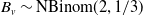 $B_v \sim \text{NBinom}(2,1/3)$
such that
$B_v \sim \text{NBinom}(2,1/3)$
such that
 $\mathbb{E}[B_v]=4$
, We let
$\mathbb{E}[B_v]=4$
, We let
 $\mathcal{T}^{\mathrm{binary}}$
grow regularly by adding levels to the binary tree structure. By Corollary 4.8, the variance of
$\mathcal{T}^{\mathrm{binary}}$
grow regularly by adding levels to the binary tree structure. By Corollary 4.8, the variance of
 $S/d$
is asymptotically dominated by that of
$S/d$
is asymptotically dominated by that of
 $S^*/d$
, defined on
$S^*/d$
, defined on
 $\mathcal{B}^{(3)}$
. Thus, by Proposition 4.6, the law of large numbers apply. Figure 5(a) shows the cdfs of
$\mathcal{B}^{(3)}$
. Thus, by Proposition 4.6, the law of large numbers apply. Figure 5(a) shows the cdfs of
 $S/d$
for progressively larger versions of the trees: we see that the distribution of
$S/d$
for progressively larger versions of the trees: we see that the distribution of
 $S/d$
becomes increasingly concentrated around its theoretical mean
$S/d$
becomes increasingly concentrated around its theoretical mean
 $\mathbb{E}[S]/d = 4$
. Next, consider
$\mathbb{E}[S]/d = 4$
. Next, consider
 $\mathcal{T}^{\mathrm{star}}$
, a star tree (as in Figure 5(b)), and let it grow by adding vertices directly to the central node (the dark vertex in Figure 4(b)). Since the resulting sequence of trees does not have uniformly bounded degree, we cannot apply Corollary 4.8. Incidentally, the cdf of
$\mathcal{T}^{\mathrm{star}}$
, a star tree (as in Figure 5(b)), and let it grow by adding vertices directly to the central node (the dark vertex in Figure 4(b)). Since the resulting sequence of trees does not have uniformly bounded degree, we cannot apply Corollary 4.8. Incidentally, the cdf of
 $S/d$
, in Figure 5(b), with
$S/d$
, in Figure 5(b), with
 $\boldsymbol{{X}}$
defined using the same parameters as before, suggests that the law of large numbers is not applicable in this case.
$\boldsymbol{{X}}$
defined using the same parameters as before, suggests that the law of large numbers is not applicable in this case.
Tree structures from Example 4.9.

Cdfs of
 $S/d$
for Example 4.9.
$S/d$
for Example 4.9.

Example 4.9 illustrates that
 $S/d$
may converge to a non-degenerate distribution as
$S/d$
may converge to a non-degenerate distribution as
 $d \to \infty$
, which has nontrivial implications for risk pooling and diversification (see, e.g., Denuit and Robert, Reference Denuit and Robert2021).
$d \to \infty$
, which has nontrivial implications for risk pooling and diversification (see, e.g., Denuit and Robert, Reference Denuit and Robert2021).
5. Estimation procedure
We describe the estimation procedure for the MPMRF frequency model, which involves constructing a correlation-based maximum spanning tree (MST) to estimate the tree structure and obtaining the maximum likelihood (ML) estimates for
 $\boldsymbol{\lambda}$
and
$\boldsymbol{\lambda}$
and
 $\boldsymbol{\alpha}$
given the resulting tree.
$\boldsymbol{\alpha}$
given the resulting tree.
5.1. Tree structure estimation
To estimate the tree structure, we construct a MST from the matrix of empirical correlations; one may use Kruskal’s algorithm for this construction (Kruskal, Reference Kruskal1956).
For Ising models with symmetric marginal distributions (i.e., with no external fields), Bresler and Karzand (Reference Bresler and Karzand2020) established that the Chow–Liu dependence tree (Chow and Liu, Reference Chow and Liu1968), which maximizes likelihood, coincides with the tree maximizing empirical correlations. This equivalence reflects the fact that, in that setting, pairwise correlation is a strictly monotone function of the Ising underlying interaction parameter. Consequently, ordering edges by mutual information or by correlation yields the same dependence tree, and the corresponding approximation minimizes the Kullback–Leibler divergence to the true distribution.
An analogous simplification arises in our context. Although the mutual information of the bivariate Poisson distribution does not admit a closed-form expression, the approximation
 $I(X_1, X_2) \approx -\ln(1 - \rho_P(X_1,X_2)),$
is strictly increasing in
$I(X_1, X_2) \approx -\ln(1 - \rho_P(X_1,X_2)),$
is strictly increasing in
 $\rho_{P}(X_1,X_2)$
and very accurate for
$\rho_{P}(X_1,X_2)$
and very accurate for
 $\rho\lt0.7$
(Guerrero-Cusumano, Reference Guerrero-Cusumano1995). Ranking edges by empirical mutual information is thus approximately equivalent to ranking them by empirical correlations. This monotonicity allows us to recover the Chow–Liu tree using correlations.
$\rho\lt0.7$
(Guerrero-Cusumano, Reference Guerrero-Cusumano1995). Ranking edges by empirical mutual information is thus approximately equivalent to ranking them by empirical correlations. This monotonicity allows us to recover the Chow–Liu tree using correlations.
A further justification arises from the small sample sizes in our numerical illustration: a sensitivity analysis (Supplement D) shows that the true tree structure is recovered more reliably if empirical correlations are used as edge weights. This behaviour is consistent with the design of the MPMRF model: edge-wise dependence is parameterized through correlations. We theoretically investigate the sample size required to recover the Chow–Liu MST in a separate working paper.
5.2. MPMRF maximum likelihood estimators
We estimate the frequency model parameters
 $(\boldsymbol{\lambda}, \boldsymbol{\alpha})$
by maximizing the log-likelihood derived from Proposition 2.6(i), under the constraints of Theorem 2.2, using numerical optimization. The maximization may be carried out using base R optim quasi-Newton BFGS algorithm, with parameter bounds enforced through a scaled logit reparametrization and a logarithmic reparametrization for the dependence parameters and marginal mean parameters, respectively. The structure of
$(\boldsymbol{\lambda}, \boldsymbol{\alpha})$
by maximizing the log-likelihood derived from Proposition 2.6(i), under the constraints of Theorem 2.2, using numerical optimization. The maximization may be carried out using base R optim quasi-Newton BFGS algorithm, with parameter bounds enforced through a scaled logit reparametrization and a logarithmic reparametrization for the dependence parameters and marginal mean parameters, respectively. The structure of
 $\boldsymbol{{N}}$
facilitates the ML estimation task: its stochastic construction separates marginal and dependence parameters, and the joint pmf (2.4) factorizes over cliques of the tree (pairs of connected vertices). As a result, ML estimation naturally aligns with the sequential procedure frequently applied in copula modeling, itself a specific instance of composite likelihood (Varin et al., Reference Varin, Reid and Firth2011). Initialization exploits the separation between frequency parameters and dependence parameters in the likelihood. Since the marginal intensities can be estimated independently of the dependence structure, the frequency parameters
$\boldsymbol{{N}}$
facilitates the ML estimation task: its stochastic construction separates marginal and dependence parameters, and the joint pmf (2.4) factorizes over cliques of the tree (pairs of connected vertices). As a result, ML estimation naturally aligns with the sequential procedure frequently applied in copula modeling, itself a specific instance of composite likelihood (Varin et al., Reference Varin, Reid and Firth2011). Initialization exploits the separation between frequency parameters and dependence parameters in the likelihood. Since the marginal intensities can be estimated independently of the dependence structure, the frequency parameters
 $\boldsymbol{\lambda}$
are first obtained by maximizing the marginal likelihood. Conditional on these estimates, the dependence parameters
$\boldsymbol{\lambda}$
are first obtained by maximizing the marginal likelihood. Conditional on these estimates, the dependence parameters
 $\boldsymbol{\alpha}$
are initialized through sequential bivariate likelihood maximization. These initial values can serve as starting points for the joint ML estimation of the full model. Since the likelihood function is invariant to the choice of root, the optimization results do not depend on a selected root vertex.
$\boldsymbol{\alpha}$
are initialized through sequential bivariate likelihood maximization. These initial values can serve as starting points for the joint ML estimation of the full model. Since the likelihood function is invariant to the choice of root, the optimization results do not depend on a selected root vertex.
6. Data illustration
We examine the applicability and performance of the MPMRF model by analyzing yearly rainfall measurements (in millimeters) from extreme events collected at weather stations in Nova Scotia. The data were sourced from the archives of Environment and Climate Change Canada (ECCC) using the weathercan package (LaZerte and Albers, Reference LaZerte and Albers2018). Our analysis is inspired by the work of Murphy and Schulz (Reference Murphy and Schulz2025), who proposed a multivariate Poisson distribution based on a triangular comonotonic shock construction (MPTCS) and applied it to annual extreme event count data from three weather stations. We compare the performance of the MPMRF frequency model, as proposed in Theorem 2.2, with the MPTCS model. Both models feature marginal Poisson distributions and account for positive dependence. Additionally, we extend our analysis to jointly model the frequency and severity of rainfall events across a portfolio of 10 weather stations using the MPMRF risk model.
To conduct our analysis, we work with three datasets. The first dataset, sourced from Murphy and Schulz (Reference Murphy and Schulz2025), consists of 71 yearly trivariate observations of extreme events recorded at three stations covering the period from 1919 to 2000. We create the second and third datasets based on three other stations and 10 stations, respectively, with data spanning from 1949 to 2000. We provide in Table 2 the complete list of weather stations included in this study. Note that some stations were moved during these periods, explaining their two climate identification numbers. The third dataset also records the rainfall amounts associated with each extreme event.
Parameters
 $\gamma_{\mathcal{W}}$
for each set
$\gamma_{\mathcal{W}}$
for each set
 $\mathcal{W}$
of vertices in Figure 2.
$\mathcal{W}$
of vertices in Figure 2.

Vertex numbers, meteorological stations, and climate ID suffixes, and the datasets in which they are used.

a All full station IDs are of the form 820xxxx.
6.1. Datasets 2 and 3 construction
We use the peak-over-threshold (POT) approach to model extreme events; see Embrechts et al. (Reference Embrechts, Klüppelberg and Mikosch1997), Chapter 6. By Theorem 7.1 of Coles (Reference Coles2001), counts of extreme events, over a sufficiently high threshold u, are Poisson distributed. The excesses
 $Y = X-u | X \gt u$
follow a generalized Pareto distribution (GPD) (Chavez-Demoulin and Davison, Reference Chavez-Demoulin and Davison2005), whose cdf is given by
$Y = X-u | X \gt u$
follow a generalized Pareto distribution (GPD) (Chavez-Demoulin and Davison, Reference Chavez-Demoulin and Davison2005), whose cdf is given by
 \begin{equation*}F_Y(y)=\begin{cases}1 - \left(1+{\xi y}/{\sigma}\right)^{-1/\xi}\!, & \xi \neq 0,\\1 - \mathrm{e}^{-{y}/{\sigma}}, & \xi=0,\end{cases}\end{equation*}
where
 $\sigma \gt0$
, and
$\sigma \gt0$
, and
 $\xi \in \mathbb{R}$
denote the scale and shape parameters of the GPD.
$\xi \in \mathbb{R}$
denote the scale and shape parameters of the GPD.
The construction of Datasets 2 and 3 requires selecting a threshold such that exceedances’ frequency and their corresponding excesses follow a Poisson and a GPD distribution, respectively, for each station. Following Thiombiano et al. (Reference Thiombiano, El Adlouni, St-Hilaire, Ouarda and El-Jabi2017), we relied on the mean-excess plot and the stability of the estimated GPD shape parameter to guide threshold selection. A chi-squared goodness-of-fit test was then applied to the excesses above the chosen threshold. We grouped exceedance-count classes so that all expected frequencies were at least 5. For all stations, the null hypothesis of a GPD distribution could not be rejected at the 20% level. We also performed Anderson–Darling tests, which confirm these conclusions. Because the threshold determines both the number of POT events and the validity of modeling assumptions, we also verified the independence of exceedances. A one-day declustering rule was applied to daily precipitation data, after which the autocorrelation function and Ljung–Box test (p-value of 5%) confirmed negligible residual dependence. For the frequency component, independence of annual exceedance counts was examined using the same diagnostics, and a chi-squared goodness-of-fit test showed that the null hypothesis of a Poisson distribution could not be rejected at the 30% level. The selected thresholds, together with the distribution of cluster sizes for each station used in Dataset 2 and 3, are reported in Table 3. The complete dataset construction procedure, along with diagnostic plots and statistical tests are provided in Supplement E.
Extreme precipitation events threshold u and distribution of cluster sizes (in days) after declustering.

6.2. Frequency models comparison
We compare the performance of the MPMRF and MPTCS frequency models for the three-station datasets. The ML estimates of the frequency means and the estimated Pearson correlations for both datasets and models are reported in Tables 4 and 5. For both datasets, the means of the MPMRF marginal distributions are exactly the empirical means, but not for MPTCS; this is because MPMRF is able to dissociate marginal and dependence modeling. In terms of dependence, for Dataset 1, the MPMRF model yields correlations that are closer to the empirical values for the edges of its tree, given by (2)–(1)–(3). In contrast, the MPTCS model performs better for the pair (2,3). For Dataset 2, the inferred dependence structure forms the tree (1)–(2)–(3), with MPMRF outperforming MPTCS on the edge (1,2). MPTCS is slightly better on edge (2,3). However, MPTCS is better at capturing the correlation within (1,3). This highlights a structural limitation of the MPMRF model: correlations between non-adjacent vertices necessarily factorize along the unique path of the tree, which restricts the maximal dependence the model can reproduce. The tree structure identifies the most influential relationships within the complete network.
Event counts estimates for Datasets 1 and 2.

Empirical (E), MPMRF (A), Murphy and Schulz (Reference Murphy and Schulz2025) (B).
Pairwise Pearson’s correlations for Datasets 1 and 2.

Empirical (E), MPMRF (A), Murphy and Schulz (Reference Murphy and Schulz2025) (B).
To compare the models formally, we use the Bayesian Information Criterion (BIC) and the corrected Akaike Information Criterion (AICc). The AICc adjusts the traditional AIC for small-sample bias, which is particularly relevant given our relatively small sample sizes (Hurvich and Tsai, Reference Hurvich and Tsai1989). It is defined as
 $\mathrm{AICc} = \mathrm{AIC} + {2k(k+1)}/{(n - k - 1)}$
. Table 6 presents the BIC and AICc values for each model across both datasets. For Dataset 1, the MPTCS model shows lower values for both criteria, indicating a better statistical fit. In contrast, for Dataset 2, the MPMRF model achieves lower values. These findings suggest that neither model consistently outperforms the other across different trivariate datasets.
$\mathrm{AICc} = \mathrm{AIC} + {2k(k+1)}/{(n - k - 1)}$
. Table 6 presents the BIC and AICc values for each model across both datasets. For Dataset 1, the MPTCS model shows lower values for both criteria, indicating a better statistical fit. In contrast, for Dataset 2, the MPMRF model achieves lower values. These findings suggest that neither model consistently outperforms the other across different trivariate datasets.
Model comparison using BIC and AICc criteria for Datasets 1 and 2.

In terms of computational performance, the MPTCS model encounters challenges in parameter estimation as the dimension increases. As discussed in Section 4 of Murphy and Schulz (Reference Murphy and Schulz2025), non-convergence may occur, particularly in scenarios with smaller sample sizes. To improve stability, the authors use a parameter grid search to initialize the sequential likelihood estimation and recommend employing multiple parameter initializations. For the three-dimensional MPTCS estimation in Dataset 2, we followed this strategy by generating 1000 random initializations of the free parameters and selecting the configuration that attained the highest sequential likelihood value. The runtime was approximately 100 s. Starting from the selected initialization, the two-step ML procedure converges in roughly 18 s, whereas the full ML estimation requires about 32 s. While this grid-search approach is feasible in lower dimensions, it becomes increasingly complex in higher dimensions. For example, achieving estimation at a dimension of
 $d = 10$
is unfeasible on a personal computer.
$d = 10$
is unfeasible on a personal computer.
In contrast, both the sequential likelihood estimation and the ML estimation of the MPMRF model on Dataset 2 require less than 1 second. The MPMRF frequency model scales well with dimension and retains interpretability in its dependence structure, as demonstrated in the subsequent risk model analysis.
6.3. MPMRF risk model on the 10-station dataset
To showcase the applicability of the MPMRF model for risk modeling in greater dimensions, we now turn to Dataset 3. We fit a risk model as in (1.1) for the rain excesses (not just the frequency of exceedances). For the frequency model, we compute the parameters’ estimates using the procedure outlined in Section 5; severities are modeled separately, given their independence with the frequency. The total runtime is less than 2 seconds.
For the marginal distributions of
 $\boldsymbol{{X}}$
, the values of the ML estimates are reported in Table 7(a). For the severity, ML estimation was produced using the QRM package of McNeil et al. (Reference McNeil, Frey and Embrechts2015). For stations where the profile likelihood 95% confidence interval for the shape parameter
$\boldsymbol{{X}}$
, the values of the ML estimates are reported in Table 7(a). For the severity, ML estimation was produced using the QRM package of McNeil et al. (Reference McNeil, Frey and Embrechts2015). For stations where the profile likelihood 95% confidence interval for the shape parameter
 $\xi$
included zero, we set
$\xi$
included zero, we set
 $\hat{\xi}=0$
and fitted an exponential distribution, following the principle of parsimony. Salmon Hole (ID 4) and Liverpool Big Falls (ID 9) exhibit high severity means and variances, making them significant from a risk modeling perspective. For diagnostics on the marginal fits, see Supplement E.4.
$\hat{\xi}=0$
and fitted an exponential distribution, following the principle of parsimony. Salmon Hole (ID 4) and Liverpool Big Falls (ID 9) exhibit high severity means and variances, making them significant from a risk modeling perspective. For diagnostics on the marginal fits, see Supplement E.4.
Parameter estimates for the frequency, severity, and dependence structure. Bootstrap standard deviations on 1000 samples are provided for
 $\boldsymbol{\lambda}$
and
$\boldsymbol{\lambda}$
and
 $\boldsymbol{\alpha}$
.
$\boldsymbol{\alpha}$
.

Regarding dependence modeling, the MST constructed from the empirical correlations is diplayed in Figure 6. Dependence parameters are reported in Table 7(b) following the ordering induced by the MST. Column 4 of Table 7(b) reports, for each edge, the ratio of the estimated dependence parameter to its corresponding maximal admissible value, from the constraint
 $\alpha_{(u, v)} \in (0, \alpha_{(u, v)}^{\max}]$
, with
$\alpha_{(u, v)} \in (0, \alpha_{(u, v)}^{\max}]$
, with
 $\alpha_{(u, v)}^{\max}\, :\!= \,\min(\sqrt{\lambda_u/\lambda_v}, \sqrt{\lambda_v/\lambda_u})$
,
$\alpha_{(u, v)}^{\max}\, :\!= \,\min(\sqrt{\lambda_u/\lambda_v}, \sqrt{\lambda_v/\lambda_u})$
,
 $(u,v)\in\mathcal{E}$
. We note that, for most edge combinations, the maximal admissible value largely exceeds the ML estimate. In Figure 7(a), we present the correlation for the frequency, with empirical correlations (lower triangle) and model-induced correlations (upper triangle). Figure 7(b) shows the analogous comparison for annual excesses
$(u,v)\in\mathcal{E}$
. We note that, for most edge combinations, the maximal admissible value largely exceeds the ML estimate. In Figure 7(a), we present the correlation for the frequency, with empirical correlations (lower triangle) and model-induced correlations (upper triangle). Figure 7(b) shows the analogous comparison for annual excesses
 $\boldsymbol{{X}}$
. Under the independence assumption for claim severities in the MPMRF risk model, the correlations ratio between
$\boldsymbol{{X}}$
. Under the independence assumption for claim severities in the MPMRF risk model, the correlations ratio between
 $\boldsymbol{{X}}$
and
$\boldsymbol{{X}}$
and
 $\boldsymbol{{N}}$
is
$\boldsymbol{{N}}$
is
 $\rho_{\boldsymbol{{X}}}(X_u,X_v)/\rho_{\boldsymbol{{N}}}(N_u,N_v) = \mathbb{E}[B_u]\mathbb{E}[B_v]/\sqrt{\mathbb{E}[B_u^2]\mathbb{E}[B_v^2]}$
for vertices
$\rho_{\boldsymbol{{X}}}(X_u,X_v)/\rho_{\boldsymbol{{N}}}(N_u,N_v) = \mathbb{E}[B_u]\mathbb{E}[B_v]/\sqrt{\mathbb{E}[B_u^2]\mathbb{E}[B_v^2]}$
for vertices
 $u,v \in \mathcal{V}$
, which ranges from 0.8541 to 0.9344. The comparison of theoretical (lower triangle) and empirical (upper triangle) pairwise correlations in Figure 7(a) illustrates the effect of path-based correlations on a tree structure. For both heatmaps, we observe clearly how the tree structure shows through the dependence captured by the model: close to the diagonal, where most edges lie, the model’s correlations are very similar to the empirical ones. However, as paths between components lengthens, the model cannot capture as much dependence due to the correlation decay feature of tree-structured MRFs: correlations between non-adjacent vertices are forced to factorize multiplicatively along the unique path of the tree.
$u,v \in \mathcal{V}$
, which ranges from 0.8541 to 0.9344. The comparison of theoretical (lower triangle) and empirical (upper triangle) pairwise correlations in Figure 7(a) illustrates the effect of path-based correlations on a tree structure. For both heatmaps, we observe clearly how the tree structure shows through the dependence captured by the model: close to the diagonal, where most edges lie, the model’s correlations are very similar to the empirical ones. However, as paths between components lengthens, the model cannot capture as much dependence due to the correlation decay feature of tree-structured MRFs: correlations between non-adjacent vertices are forced to factorize multiplicatively along the unique path of the tree.
Correlation-based maximum spanning tree of 10 meteorological stations in Nova Scotia.

Correlation heatmaps of yearly extreme precipitation events counts (left) and amounts (right) comparing empirical (lower triangle) and theoretical (upper triangle).

Despite the cost of reduced flexibility in capturing long-range or higher-order interactions, the tree structure confers substantial analytical tractability, enabling closed-form likelihood evaluation, scalable inference, and efficient computation of portfolio-level risk measures. It is also interpretable: Figure 6 confirms the nontrivial spatial-dependence channels through which yearly extreme events co-vary.
We next proceed to perform the two risk management tasks discussed in Sections 3 and 4 for the obtained MPMRF model. The first risk management task is to assess the distribution of S and measure the risk. We proceed using discretization methods. Let
 $\widetilde{B}$
be the discretized version of a continuous severity random variable B. If
$\widetilde{B}$
be the discretized version of a continuous severity random variable B. If
 $B \sim \mathrm{GPD}(\xi, \sigma;\; u)$
, then
$B \sim \mathrm{GPD}(\xi, \sigma;\; u)$
, then
 $\widetilde{B}$
follows a discretized generalized Pareto distribution (DGPD) with parameters
$\widetilde{B}$
follows a discretized generalized Pareto distribution (DGPD) with parameters
 $(\xi, \sigma;\; u)$
, with
$(\xi, \sigma;\; u)$
, with
 $p_{\widetilde{B}}(x) = \overline{F}_{B}(x h) - \overline{F}_{B}((x + 1)h)$
, for every
$p_{\widetilde{B}}(x) = \overline{F}_{B}(x h) - \overline{F}_{B}((x + 1)h)$
, for every
 $x \in \{u + h\;:\; h\in\mathbb{N}\}$
where
$x \in \{u + h\;:\; h\in\mathbb{N}\}$
where
 $\overline{F}$
denotes the survival function and h is the discretization step. For the use of the DGPD in a practical context, see Prieto et al. (Reference Prieto, Gómez-Déniz and Sarabia2014). We use this specification for the severity component in our portfolio analysis with
$\overline{F}$
denotes the survival function and h is the discretization step. For the use of the DGPD in a practical context, see Prieto et al. (Reference Prieto, Gómez-Déniz and Sarabia2014). We use this specification for the severity component in our portfolio analysis with
 $h = 0.1$
, as the dataset’s total rainfall is reported on a decimal scale. Using the FFT algorithm, we obtain the distribution of the discretized aggregate loss, denoted
$h = 0.1$
, as the dataset’s total rainfall is reported on a decimal scale. Using the FFT algorithm, we obtain the distribution of the discretized aggregate loss, denoted
 $\widetilde{S}$
. Table 8 summarizes key portfolio-level statistics and compares them with those obtained using the assumption of independent compound Poisson distributions. The marked differences illustrate the critical role of dependence in the frequency component for an accurate assessment of portfolios’ risks.
$\widetilde{S}$
. Table 8 summarizes key portfolio-level statistics and compares them with those obtained using the assumption of independent compound Poisson distributions. The marked differences illustrate the critical role of dependence in the frequency component for an accurate assessment of portfolios’ risks.
Characteristics and risk measures for
 $\widetilde{S}$
, with comparison to the independent case,
$\widetilde{S}$
, with comparison to the independent case,
 $\widetilde{S}^{\perp\!\!\!\perp}$
. Values are rounded to the nearest whole number.
$\widetilde{S}^{\perp\!\!\!\perp}$
. Values are rounded to the nearest whole number.

The second risk management task is to analyze how each station individually contributes to the total risk. We use the TVaR allocation principle in (4.1). We compute the TVaR contributions for each vertex in the frequency and compound model using the method based on OGFEAs from Section 4. These contributions are denoted as
 $ C^{\mathrm{TVaR}}_{\kappa}(N_v;\;M) $
and
$ C^{\mathrm{TVaR}}_{\kappa}(N_v;\;M) $
and
 $ C^{\mathrm{TVaR}}_{\kappa}(\widetilde{X}_v;\;\widetilde{S}) $
, respectively. Figure 8 illustrates the relative contributions to
$ C^{\mathrm{TVaR}}_{\kappa}(\widetilde{X}_v;\;\widetilde{S}) $
, respectively. Figure 8 illustrates the relative contributions to
 $ \mathrm{TVaR}_{\kappa}(M) $
and
$ \mathrm{TVaR}_{\kappa}(M) $
and
 $ \mathrm{TVaR}_{\kappa}(\widetilde{S}) $
from each station.
$ \mathrm{TVaR}_{\kappa}(\widetilde{S}) $
from each station.
Relative contributions to
 $\text{TVaR}_{\kappa}(Z)$
, using the frequency vector
$\text{TVaR}_{\kappa}(Z)$
, using the frequency vector
 $\boldsymbol{{N}} \; (Z = M)$
and the risk model vector
$\boldsymbol{{N}} \; (Z = M)$
and the risk model vector
 $\boldsymbol{{X}} \; (Z = S)$
.
$\boldsymbol{{X}} \; (Z = S)$
.

By examining Figure 8(a), we observe that stations Upper Stewiacke (ID 2) and Yarmouth (ID 10) have a more significant impact on the overall frequency distribution, which is consistent with their high-frequency mean parameters. For Figure 8(b), which incorporates both the frequency and severity components, Liverpool Big Falls (ID 9) emerges as the dominant contributor across all values of
 $\kappa$
. This behavior is driven by the combination of its relatively high mean frequency parameter and its large severity mean and variance (compared to other stations), as reported in Table 7(a). Indeed, a comparison between Figure 8(a) and (b) reveals that, while the shape of the relative contribution curves remains consistent, the curves are shifted vertically depending on the combined frequence-severity distributions.
$\kappa$
. This behavior is driven by the combination of its relatively high mean frequency parameter and its large severity mean and variance (compared to other stations), as reported in Table 7(a). Indeed, a comparison between Figure 8(a) and (b) reveals that, while the shape of the relative contribution curves remains consistent, the curves are shifted vertically depending on the combined frequence-severity distributions.
The relative contribution to aggregate risk of certain random variables decreases as the
 $ \kappa $
value increases. Locations connected to the tree through weaker (and fewer) edge correlations exhibit declining relative importance as
$ \kappa $
value increases. Locations connected to the tree through weaker (and fewer) edge correlations exhibit declining relative importance as
 $\kappa$
increases, reflecting their limited dependence with other vertices. Conversely, locations connected by strong edges and occupying central positions in the MST show increasing contributions at higher
$\kappa$
increases, reflecting their limited dependence with other vertices. Conversely, locations connected by strong edges and occupying central positions in the MST show increasing contributions at higher
 $\kappa$
values. This observation offers critical insights for modeling. By examining the correlation edges of each vertex within the dependence structure, risk modelers can predict which components of the portfolio will see increased relative contributions as they move further into the tail of the aggregate risk distribution. Most notably, Salmon Hole (ID 4) demonstrates the steepest upward trend across
$\kappa$
values. This observation offers critical insights for modeling. By examining the correlation edges of each vertex within the dependence structure, risk modelers can predict which components of the portfolio will see increased relative contributions as they move further into the tail of the aggregate risk distribution. Most notably, Salmon Hole (ID 4) demonstrates the steepest upward trend across
 $\kappa$
values. As a consequence of both high severity and its globally influential correlations within the tree (see Table 6), Salmon Hole’s ranking in relative TVaR
$\kappa$
values. As a consequence of both high severity and its globally influential correlations within the tree (see Table 6), Salmon Hole’s ranking in relative TVaR
 $_{0.99}$
contribution rises from 9th (frequency alone) to 6th (frequency-severity).
$_{0.99}$
contribution rises from 9th (frequency alone) to 6th (frequency-severity).
To compare allocations to vertices using different principles, we evaluate the contribution of each risk under both covariance-based and TVaR-based allocation rules. This comparison is illustrated in Figure 9, which shows the contributions of each station by scaling vertex sizes based on: (a) the covariance-based allocation
 $ C^{\mathrm{Cov}}_\kappa({X_v}, {S}) $
and (b) the TVaR-based allocation
$ C^{\mathrm{Cov}}_\kappa({X_v}, {S}) $
and (b) the TVaR-based allocation
 $ C^{\mathrm{TVaR}}_\kappa(\widetilde{X_v}, \widetilde{S}) $
, for each
$ C^{\mathrm{TVaR}}_\kappa(\widetilde{X_v}, \widetilde{S}) $
, for each
 $ v \in \mathcal{V} $
and
$ v \in \mathcal{V} $
and
 $ \kappa = 0.99 $
. In both cases, scaling is performed relative to the portfolio’s TVaR. As a benchmark, panel (c) displays the relative contribution of each station’s marginal mean to the portfolio expectation
$ \kappa = 0.99 $
. In both cases, scaling is performed relative to the portfolio’s TVaR. As a benchmark, panel (c) displays the relative contribution of each station’s marginal mean to the portfolio expectation
 $ \mathbb{E}[{S}] $
. Note that we compute
$ \mathbb{E}[{S}] $
. Note that we compute
 $ C^{\mathrm{Cov}}_\kappa(X_v, S) $
exactly using Proposition 4.5. Supplement F complements Figure 9 by reporting the contributions and their differences, confirming that
$ C^{\mathrm{Cov}}_\kappa(X_v, S) $
exactly using Proposition 4.5. Supplement F complements Figure 9 by reporting the contributions and their differences, confirming that
 $C^{\mathrm{TVaR}}_\kappa(X_v, S)$
and
$C^{\mathrm{TVaR}}_\kappa(X_v, S)$
and
 $C^{\mathrm{Cov}}_\kappa(X_v, S)$
are close.
$C^{\mathrm{Cov}}_\kappa(X_v, S)$
are close.
 $\mathcal{T}$
with vertex sizes scaled based on (a)
$\mathcal{T}$
with vertex sizes scaled based on (a)
 $C^{\mathrm{Cov}}_{0.99}(X_v, S)$
, (b)
$C^{\mathrm{Cov}}_{0.99}(X_v, S)$
, (b)
 $C^{\mathrm{TVaR}}_{0.99}(\widetilde{X}_v, \widetilde{S})$
, and (c)
$C^{\mathrm{TVaR}}_{0.99}(\widetilde{X}_v, \widetilde{S})$
, and (c)
 $\mathbb{E}[X_v]$
.
$\mathbb{E}[X_v]$
.

7. Conclusion
We have examined the risk model in (1.1) wherein we introduced dependence between the claim counts using distributions from the family
 $\mathbb{MPMRF}$
. We established that
$\mathbb{MPMRF}$
. We established that
 $\mathbb{MPMRF}$
is a subset of
$\mathbb{MPMRF}$
is a subset of
 $\mathbb{MPCS}$
, but its specific parameterization enables more tractable analysis of high-dimensional models with Poisson marginals. We discussed two risk management tasks. First, we provided tools for analyzing the aggregate claim amount S of a portfolio. Second, we investigated risk allocation, providing analytical expression of expected allocations and methods for exact computations of risk allocations. We discussed linear risk sharing for infinite-size portfolios and showed convergence in probability of the average risk amount if the tree’s radius becomes large. We described estimation procedures for the model’s parameter. Finally, we illustrated our findings through a real data analysis.
$\mathbb{MPCS}$
, but its specific parameterization enables more tractable analysis of high-dimensional models with Poisson marginals. We discussed two risk management tasks. First, we provided tools for analyzing the aggregate claim amount S of a portfolio. Second, we investigated risk allocation, providing analytical expression of expected allocations and methods for exact computations of risk allocations. We discussed linear risk sharing for infinite-size portfolios and showed convergence in probability of the average risk amount if the tree’s radius becomes large. We described estimation procedures for the model’s parameter. Finally, we illustrated our findings through a real data analysis.
Further research can be undertaken on this family of risk models. Tighter and more general asymptotic results for risk sharing rules, in the spirit of Denuit et al. (Reference Denuit, Dhaene and Robert2022), could be established. Incorporating dependence among the severity random variables could further enhance the risk model’s use. Focusing on the frequency component, the separation between marginal distributions and the dependence structure naturally lends itself to extensions within the framework of generalized linear models (e.g., Poisson regression with log-linear link). The framework could also be broadened to other distributional families.
A potential limitation of the proposed risk model is the underestimation of correlations between non-adjacent vertices in real-data applications. Analysis of the statistical frequency model indicated that, while the model performs well on edges, it tends to underestimate correlations for non-adjacent pairs. Non-adjacent correlations may be better captured by modeling residual dependence through an auxiliary tree.
Supplementary material
The supplementary material for this article can be found at https://doi.org/10.1017/asb.2026.10087
Acknowledgements
We would like to thank three anonymous referees and the handling editor for precious comments that helped improve the quality of the paper. This work was partially supported by the Natural Sciences and Engineering Research Council of Canada (Cossette: RGPIN-2025-04077; Marceau: RGPIN-2020-05605; Côté: 581589859, Dubeau: BESC-M) and by the Chaire en actuariat de l’Université Laval (Marceau).
Data availability statement
The data and code will be made available upon request.
Competing interests
The authors have no potential competing or conflicting interests to declare.
Appendix
A. Proofs
A.1. Proof of Theorem 2.2
First, we argue that
 $\boldsymbol{{N}}$
is a MRF. The construction given in (2.2) is akin to the one presented in Theorem 1 of Côté et al. (Reference Côté, Cossette and Marceau2025b) about the stochastic dynamics at play. The arguments provided for the proof of that theorem remain relevant: the maximum information about a random variable
$\boldsymbol{{N}}$
is a MRF. The construction given in (2.2) is akin to the one presented in Theorem 1 of Côté et al. (Reference Côté, Cossette and Marceau2025b) about the stochastic dynamics at play. The arguments provided for the proof of that theorem remain relevant: the maximum information about a random variable
 $N_v$
,
$N_v$
,
 $v \in \mathcal{V}$
, is obtained by knowing the value of its neighbors. Thus, it satisfies the local Markov property, meaning
$v \in \mathcal{V}$
, is obtained by knowing the value of its neighbors. Thus, it satisfies the local Markov property, meaning
 $\boldsymbol{{N}}$
is a MRF.
$\boldsymbol{{N}}$
is a MRF.
We next prove by induction that
 $N_v\sim\text{Poisson}(\lambda_v)$
for all
$N_v\sim\text{Poisson}(\lambda_v)$
for all
 $v \in \mathcal{V}$
, with the root r as the starting point; evidently,
$v \in \mathcal{V}$
, with the root r as the starting point; evidently,
 $N_r\sim \text{Poisson}(\lambda_r)$
. We next suppose the statement holds true for
$N_r\sim \text{Poisson}(\lambda_r)$
. We next suppose the statement holds true for
 $N_{\mathrm{pa}(w)}$
,
$N_{\mathrm{pa}(w)}$
,
 $w \in \mathcal{V} \backslash \{r\}$
, and prove
$w \in \mathcal{V} \backslash \{r\}$
, and prove
 $N_w\sim\text{Poisson}(\lambda_w)$
. Following the construction in (2.2),
$N_w\sim\text{Poisson}(\lambda_w)$
. Following the construction in (2.2),
 $L_w$
is independent of all
$L_w$
is independent of all
 $L_v,\,v \in \mathcal{V}\backslash\{w\}$
and of
$L_v,\,v \in \mathcal{V}\backslash\{w\}$
and of
 $N_{\mathrm{pa}(w)}$
, since
$N_{\mathrm{pa}(w)}$
, since
 $w \not\in \mathrm{path}(\mathrm{pa}(w), r)$
. It follows that the pgf of
$w \not\in \mathrm{path}(\mathrm{pa}(w), r)$
. It follows that the pgf of
 $N_w$
is given by
$N_w$
is given by
 \begin{equation*}\mathcal{P}_{N_w}(t) = \mathcal{P}_{\left(\alpha_{(\mathrm{pa}(w), w)}\sqrt{{\lambda_w}/{\lambda_{\mathrm{pa}(w)}}} \right)\circ N_{\mathrm{pa}(w)}}(t) \mathcal{P}_{L_w}(t), \quad t \in [\!-1, 1].\end{equation*}
From the properties of the binomial thinning operator (one may refer to Theorem 11(d) of Côté et al. Reference Côté, Cossette and Marceau2025b), we have
 \begin{align}\notag\mathcal{P}_{N_w}(t) &= \mathcal{P}_{N_{\mathrm{pa}(w)}}\Big(1 - \alpha_{(\mathrm{pa}(w), w)}\sqrt{{\lambda_w}/{\lambda_{\mathrm{pa}(w)}}} + \alpha_{(\mathrm{pa}(w), w)}\sqrt{{\lambda_w}/{\lambda_{\mathrm{pa}(w)}}}t\Big) \mathcal{P}_{L_w}(t)\\&= \mathrm{e}^{\lambda_{\mathrm{pa}(w)}\left(1 + \alpha_{(\mathrm{pa}(w), w)}\sqrt{{\lambda_w}/{\lambda_{\mathrm{pa}(w)}}}(t - 1) - 1\right)} \mathrm{e}^{\left(\lambda_w - \alpha_{(\mathrm{pa}(w), w)}\sqrt{\lambda_{\mathrm{pa}(w)}\lambda_w}\right)(t - 1)}, \quad t \in [\!-1, 1], \end{align}
from the respective pgfs of
 $L_w$
and
$L_w$
and
 $N_{\mathrm{pa}(w)}$
given the induction hypothesis. Simplifying (A1) provides
$N_{\mathrm{pa}(w)}$
given the induction hypothesis. Simplifying (A1) provides
 $\mathcal{P}_{N_w}(t) = \mathrm{e}^{\lambda_w(t - 1)}$
,
$\mathcal{P}_{N_w}(t) = \mathrm{e}^{\lambda_w(t - 1)}$
,
 $t \in [\!-1, 1]$
; thus,
$t \in [\!-1, 1]$
; thus,
 $N_w \sim \mathrm{Poisson}(\lambda_w)$
. The assertion is validated for both the case of the root and the parent–child inductive case; we conclude
$N_w \sim \mathrm{Poisson}(\lambda_w)$
. The assertion is validated for both the case of the root and the parent–child inductive case; we conclude
 $N_v\sim\text{Poisson}(\lambda_v)$
for every
$N_v\sim\text{Poisson}(\lambda_v)$
for every
 $v\in\mathcal{V}$
.
$v\in\mathcal{V}$
.
Conditioning on
 $N_{\mathrm{pa}(v)}$
and using (2.2), the joint pgf of two neighbors
$N_{\mathrm{pa}(v)}$
and using (2.2), the joint pgf of two neighbors
 $(N_{\mathrm{pa}(v)}, N_v)$
is given by
$(N_{\mathrm{pa}(v)}, N_v)$
is given by
 \begin{equation*}\mathcal{P}_{N_{\mathrm{pa}(v)}, N_v}(t_{\mathrm{pa}(v)}, t_v) = \mathrm{e}^{\lambda_{\mathrm{pa}(v)}(t_{\mathrm{pa}(v)} - 1) + \lambda_v(t_v - 1) + \alpha_{(\mathrm{pa}(v), v)}\sqrt{\lambda_{\mathrm{pa}(v)}\lambda_v}(t_v - 1)(t_{\mathrm{pa}(v)} - 1)}, \quad t_{\mathrm{pa}(v)}, t_v \in [\!-1,1].\end{equation*}
Since
 $\mathcal{P}_{N_{\mathrm{pa}(v)}, N_v}(t_{\mathrm{pa}(v)}, t_v)$
is symmetric regarding
$\mathcal{P}_{N_{\mathrm{pa}(v)}, N_v}(t_{\mathrm{pa}(v)}, t_v)$
is symmetric regarding
 $N_{\mathrm{pa}(v)}$
and
$N_{\mathrm{pa}(v)}$
and
 $N_v$
, the stochastic dynamics on an edge are reversible. Given the local Markov property, this reversibility extends to the stochastic dynamics on a path. Moreover, note that choosing a root
$N_v$
, the stochastic dynamics on an edge are reversible. Given the local Markov property, this reversibility extends to the stochastic dynamics on a path. Moreover, note that choosing a root
 $r'\neq r$
only affects the parent–child relationships of the vertices on
$r'\neq r$
only affects the parent–child relationships of the vertices on
 $\mathrm{path}(r, r')$
. Other vertices remain children to their parent, with unchanged stochastic dynamics.
$\mathrm{path}(r, r')$
. Other vertices remain children to their parent, with unchanged stochastic dynamics.
A.2. Proof of Proposition 2.6
The proof resembles those of Theorems 3 and 4 of Côté et al. (Reference Côté, Cossette and Marceau2025b) and is thus omitted.
A.3. Proof of Proposition 2.7
The choice of the root has no incidence on the distribution of
 $\boldsymbol{{N}}$
(Theorem 2.2). For all
$\boldsymbol{{N}}$
(Theorem 2.2). For all
 $v\in\mathcal{V}$
, we have
$v\in\mathcal{V}$
, we have
 \begin{equation} \eta_v^{\mathcal{T}_r}(\boldsymbol{{t}}_{v\mathrm{dsc}(v)};\;\boldsymbol{\theta}_{\mathrm{dsc}(v)}) = t_v \sum_{\mathcal{C} \in \mathscr{P}(\mathrm{ch}(v))} \left(\prod_{j\in \mathrm{ch}(v)\backslash \mathcal{W}} (1-\theta_j) \right) \left(\prod_{i \in \mathcal{W}} \theta_i \eta_i^{\mathcal{T}_r}(\boldsymbol{{t}}_{i\mathrm{dsc}(i)};\;\boldsymbol{\theta}_{\mathrm{dsc}(i)}) \right)\!. \end{equation}
Let
 $\Xi_v = \{\mathcal{W}\cap v\mathrm{dsc}(v) : \mathcal{W}\in\Theta_v\}$
. Write
$\Xi_v = \{\mathcal{W}\cap v\mathrm{dsc}(v) : \mathcal{W}\in\Theta_v\}$
. Write
 $\mathrm{ch}^{i}(v)$
to refer to the ith generation of the descendants of v,
$\mathrm{ch}^{i}(v)$
to refer to the ith generation of the descendants of v,
 $i\in\mathbb{N}$
; for instance,
$i\in\mathbb{N}$
; for instance,
 $\mathrm{ch}^2(v)$
are the children of the children of v. Let
$\mathrm{ch}^2(v)$
are the children of the children of v. Let
 $\Xi_v^{[i]} = \{\mathcal{W}\cap \mathrm{ch}^{i}(v) : \mathcal{W}\in\Xi_v\}$
. From (A2), we use the result recursively to further develop
$\Xi_v^{[i]} = \{\mathcal{W}\cap \mathrm{ch}^{i}(v) : \mathcal{W}\in\Xi_v\}$
. From (A2), we use the result recursively to further develop
 $\eta_{v}^{\mathcal{T}_v}$
, yielding after one iteration
$\eta_{v}^{\mathcal{T}_v}$
, yielding after one iteration
 \begin{align} &\eta_v^{\mathcal{T}_r}(\boldsymbol{{t}}_{v\mathrm{dsc}(v)};\;\boldsymbol{\theta}_{\mathrm{dsc}(v)})\notag \\ &= t_v \sum_{\mathcal{W} \in \Xi_v^{[2]}} \left(\prod_{j\in \mathrm{ch}(v)\backslash \mathcal{C}} (1-\theta_j) \right) \left(\prod_{i \in \mathcal{C}} \theta_i t_i \left(\prod_{k\in \mathrm{ch}(i)\backslash \mathcal{W}} (1-\theta_k) \right) \left(\prod_{\ell \in \mathrm{ch}(i)\cup \mathcal{W}} \theta_\ell \eta_i^{\mathcal{T}_r}(\boldsymbol{{t}}_{i\mathrm{dsc}(i)};\;\boldsymbol{\theta}_{\mathrm{dsc}(i)}) \right)\right)\notag\\ &= t_v \sum_{\mathcal{W}\in \Xi^{[2]}_v} \left(\prod_{(\mathrm{pa}(j),j)\in\mathcal{E}^{\dagger}_{\mathcal{W}}} (1-\theta_j) \right) \left(\prod_{(\mathrm{pa}(i),i)\in\mathcal{E}_{\mathcal{W}}} \theta_i t_i\right) \left(\prod_{\ell\in \mathrm{ch}^2(i)} \frac{1}{t_\ell} \eta_{\ell}^{\mathcal{T}_r}(\boldsymbol{{t}}_{\ell\mathrm{dsc}(\ell)};\;\boldsymbol{\theta}_{\mathrm{dsc}(\ell)})\right)\!. \end{align}
Continuing recursively in this fashion down to the bottom of the tree (say it takes
 $m\in\mathbb{N}$
iterations), we have
$m\in\mathbb{N}$
iterations), we have
 $\Xi^{[m]}_v = \Xi_v$
, and (A3) becomes
$\Xi^{[m]}_v = \Xi_v$
, and (A3) becomes
 \begin{equation} \eta_v^{\mathcal{T}_r}(\boldsymbol{{t}}_{v\mathrm{dsc}(v)};\;\boldsymbol{\theta}_{\mathrm{dsc}(v)}) = t_v \sum_{\mathcal{W}\in\Xi_v} \left(\prod_{(\mathrm{pa}(j),j)\in\mathcal{E}^{\dagger}_{\mathcal{W}}} (1-\theta_j) \right) \left(\prod_{(\mathrm{pa}(i),i)\in\mathcal{E}_{\mathcal{W}}} \theta_i t_i\right)\!, \end{equation}
since
 $\eta_{\ell}^{\mathcal{T}_r}(\boldsymbol{{t}}_{\ell\mathrm{dsc}(\ell)};\;\boldsymbol{\theta}_{\mathrm{dsc}(\ell)}) = t_{\ell}$
for every
$\eta_{\ell}^{\mathcal{T}_r}(\boldsymbol{{t}}_{\ell\mathrm{dsc}(\ell)};\;\boldsymbol{\theta}_{\mathrm{dsc}(\ell)}) = t_{\ell}$
for every
 $\ell\in \xi_v^{[m]}$
. Inserting (A4) into (2.5),
$\ell\in \xi_v^{[m]}$
. Inserting (A4) into (2.5),
 $\mathcal{P}_{\boldsymbol{{N}}}$
is thus given by
$\mathcal{P}_{\boldsymbol{{N}}}$
is thus given by
 \begin{equation} \mathcal{P}_{\boldsymbol{{N}}}(\boldsymbol{{t}}) = \prod_{v\in\mathcal{V}} \prod_{\mathcal{W}\in \Xi_v} \mathrm{e}^{\zeta_{L_v} \left(\prod_{(\mathrm{pa}(j),j)\in\mathcal{E}^{\dagger}_{\mathcal{W}}} (1-\theta_j) \right) \left(\prod_{(\mathrm{pa}(i),i)\in\mathcal{E}_{\mathcal{W}}} \theta_i t_i\right)t_v -1}, \quad \boldsymbol{{t}}\in[\!-1,1]^{d}, \end{equation}
where
 $\{\zeta_{L_v}, \, v\in\mathcal{V}\}$
and
$\{\zeta_{L_v}, \, v\in\mathcal{V}\}$
and
 $\{\theta_v,\, v\in\mathcal{V}\}$
are defined as in Proposition 2.6. Note that from the construction of
$\{\theta_v,\, v\in\mathcal{V}\}$
are defined as in Proposition 2.6. Note that from the construction of
 $\Xi_v$
, no combination of
$\Xi_v$
, no combination of
 $t_v$
’s is repeated across the product operations. One recognizes in (A5) the joint pgf of the sum of independent Poisson random vectors of the form
$t_v$
’s is repeated across the product operations. One recognizes in (A5) the joint pgf of the sum of independent Poisson random vectors of the form
 $\boldsymbol{{Y}}_{\mathcal{W}} = (Y_{\mathcal{W}}\unicode{x1D7D9}_{v\in\mathcal{W}} ,\, v\in\mathcal{V})$
, one for each element of
$\boldsymbol{{Y}}_{\mathcal{W}} = (Y_{\mathcal{W}}\unicode{x1D7D9}_{v\in\mathcal{W}} ,\, v\in\mathcal{V})$
, one for each element of
 $\bigcup_{v\in\mathcal{V}} \Xi_v = \bigcup_{v\in\mathcal{V}} \Theta_v$
, where the frequency parameter associated with
$\bigcup_{v\in\mathcal{V}} \Xi_v = \bigcup_{v\in\mathcal{V}} \Theta_v$
, where the frequency parameter associated with
 $Y_{\mathcal{W}}$
is
$Y_{\mathcal{W}}$
is
 \begin{equation} \gamma_{\mathcal{W}} = \zeta_{L_v} \left(\prod_{(\mathrm{pa}(j),j)\in\mathcal{E}^{\dagger}_{\mathcal{W}}} (1-\theta_j) \right) \left(\prod_{(\mathrm{pa}(i),i)\in\mathcal{E}_{\mathcal{W}}} \theta_i\right)\!, \quad \mathcal{W} \in \bigcup_{v\in\mathcal{V}} \Theta_v, \end{equation}
where v is the utmost vertex in
 $\mathcal{W}$
according to the rooting in r. Equation (A6) is equivalent to (2.8) after substituting back to the original parameters.
$\mathcal{W}$
according to the rooting in r. Equation (A6) is equivalent to (2.8) after substituting back to the original parameters.
A.4. Proof of Remark 3.1
The techniques for that matter are inspired from the work in Willmot and Lin (Reference Willmot and Lin2011). The cdf and LST of
 $B_v$
,
$B_v$
,
 $v \in \mathcal{V}$
, are given respectively by
$v \in \mathcal{V}$
, are given respectively by
 \begin{equation*}F_{B_v}(x) = \sum_{k=1}^{\infty} \pi_{v,k} H(x;\; k, \beta_v) \quad x \geq 0, \quad\mathcal{L}_{B_v}(t) = \sum_{k = 1}^{\infty} \pi_{v,k} \left(\frac{\beta_v}{\beta_v + t}\right)^k, \quad t \gt 0,\end{equation*}
where
 $H(x;\; k, \beta_v) = 1 - \mathrm{e}^{-\beta_v x} \sum_{l=0}^{k-1} \frac{(\beta_v x)^l}{l!}$
,
$H(x;\; k, \beta_v) = 1 - \mathrm{e}^{-\beta_v x} \sum_{l=0}^{k-1} \frac{(\beta_v x)^l}{l!}$
,
 $x \geq 0$
, is the cdf of the kth Erlang distribution with rate
$x \geq 0$
, is the cdf of the kth Erlang distribution with rate
 $\beta_v$
.
$\beta_v$
.
To reformulate
 $\mathcal{L}_S$
in (3.2), we first express every
$\mathcal{L}_S$
in (3.2), we first express every
 $\mathcal{L}_{B_v}$
according to the maximum rate parameter
$\mathcal{L}_{B_v}$
according to the maximum rate parameter
 $\beta_{\max} \, :\!= \,\max\{\beta_v \;:\; v\in \mathcal{V}\}$
. Let
$\beta_{\max} \, :\!= \,\max\{\beta_v \;:\; v\in \mathcal{V}\}$
. Let
 $v_{\max} \, :\!= \, \mathrm{argmax}\{\beta_v : v\in \mathcal{V}\}$
. For
$v_{\max} \, :\!= \, \mathrm{argmax}\{\beta_v : v\in \mathcal{V}\}$
. For
 $v \in \mathcal{V} \backslash \{v_{\max}\}$
, we can express
$v \in \mathcal{V} \backslash \{v_{\max}\}$
, we can express
 $\mathcal{L}_{B_v}$
as
$\mathcal{L}_{B_v}$
as
 \begin{equation} \mathcal{L}_{B_v}(t) = \sum_{k = 1}^{\infty} \pi_{v, k} \left[ \frac{q_v}{1 - (1 - q_v) \left(\frac{\beta_{\max}}{\beta_{\max} + t}\right)}\left(\frac{\beta_{\max}}{\beta_{\max}+ t}\right) \right]^k = \sum_{k = 1}^{\infty} \pi_{v, k} \mathcal{P}_{K_{v,k}}\left(\frac{\beta_{\max}}{\beta_{\max}+ t}\right)\!, \quad t \geq 0,\end{equation}
where
 $K_{v, k}$
follows a negative binomial distribution with number of successful trials k and success probability
$K_{v, k}$
follows a negative binomial distribution with number of successful trials k and success probability
 $q_v ={\beta_v}/{\beta_{\max}}$
. For all
$q_v ={\beta_v}/{\beta_{\max}}$
. For all
 $v \in \mathcal{V}$
, we may write
$v \in \mathcal{V}$
, we may write
 $\mathcal{L}_{B_v}(t) = \mathcal{P}_{\widetilde{K}_v}(\mathcal{L}_{B_{\max}}(t))$
, corresponding to a compound distribution with primary distribution given by the random variable
$\mathcal{L}_{B_v}(t) = \mathcal{P}_{\widetilde{K}_v}(\mathcal{L}_{B_{\max}}(t))$
, corresponding to a compound distribution with primary distribution given by the random variable
 $\widetilde{K}_v$
with pmf
$\widetilde{K}_v$
with pmf
 $p_{\widetilde{K}_v}(x) = \sum_{k=1}^\infty \pi_{v,k} \, p_{K_{v,k}}(x)$
,
$p_{\widetilde{K}_v}(x) = \sum_{k=1}^\infty \pi_{v,k} \, p_{K_{v,k}}(x)$
,
 $x \in \mathbb{N}_1$
, and secondary distribution
$x \in \mathbb{N}_1$
, and secondary distribution
 $B_{\max} \sim \mathrm{Exp}(\beta_{\max})$
. The result follows inserting (A7) in (3.2).
$B_{\max} \sim \mathrm{Exp}(\beta_{\max})$
. The result follows inserting (A7) in (3.2).
A.5. Proof of Theorem 4.2
From Theorem 3.4 of Blier-Wong et al. (Reference Blier-Wong, Cossette and Marceau2025) and (3.1), taking v as the root for the joint pgf of
 $\boldsymbol{{X}}$
,
$\boldsymbol{{X}}$
,
 \begin{align}\notag \mathcal{P}_S^{[v]}(t) &= \left.\left[t_v \frac{\partial}{\partial t_v}\mathcal{P}_{\boldsymbol{{X}}}(\boldsymbol{{t}}) \right]\right|_{\boldsymbol{{t}}=t\mathbf{1}_d} \\ &= t \left.\left[ \frac{\partial}{\partial t_v}\mathrm{e}^{\lambda_v \eta_v^{\mathcal{T}_v}\left(\boldsymbol{\mathcal{P}}_{B_v}(\boldsymbol{{t}}_{v\mathrm{dsc}(v)});\; \boldsymbol{\theta}^{\mathcal{T}_v}_{\mathrm{dsc}(v)}\right)} \prod_{j\in\mathcal{V}\backslash\{v\}} \mathrm{e}^{\zeta_{L_j} \eta_j^{\mathcal{T}_v}\left(\boldsymbol{\mathcal{P}}_{B_j}(\boldsymbol{{t}}_{j\mathrm{dsc}(j)});\; \boldsymbol{\theta}^{\mathcal{T}_v}_{\mathrm{dsc}(j)}\right)}\right]\right|_{\boldsymbol{{t}}=t\mathbf{1}_d}, \end{align}
for
 $t\in[\!-1,1]$
, where
$t\in[\!-1,1]$
, where
 $\zeta_{L_j} = \lambda_j (1-\alpha_{(\mathrm{pa}(j),j)}\sqrt{\lambda_{\mathrm{pa}(j)}/ \lambda_j} )$
. We choose v as the root for
$\zeta_{L_j} = \lambda_j (1-\alpha_{(\mathrm{pa}(j),j)}\sqrt{\lambda_{\mathrm{pa}(j)}/ \lambda_j} )$
. We choose v as the root for
 $\mathcal{P}_{\boldsymbol{{X}}}$
as it simplifies the differentiation and has no incidence on the result. All the multiplicands in (A8) are free of
$\mathcal{P}_{\boldsymbol{{X}}}$
as it simplifies the differentiation and has no incidence on the result. All the multiplicands in (A8) are free of
 $t_v$
since, if v is the root,
$t_v$
since, if v is the root,
 $v\not\in j\mathrm{dsc}(j)$
for every other
$v\not\in j\mathrm{dsc}(j)$
for every other
 $j\in\mathcal{V}\backslash\{v\}$
. Performing the differentiation in (A8) yields
$j\in\mathcal{V}\backslash\{v\}$
. Performing the differentiation in (A8) yields
 \begin{align*}\mathcal{P}_{S}^{[v]}(t) &= \lambda_v t \left.\left[ \frac{\partial}{\partial t_v}\eta_v^{\mathcal{T}_v}(\pmb{\mathcal{P}}_{B_v}(\boldsymbol{{t}}_{v\mathrm{dsc}(v)});\; \boldsymbol{\theta}^{\mathcal{T}_v}_{\mathrm{dsc}(v)})\right]\right|_{\boldsymbol{{t}}=t\mathbf{1}_d} \prod_{j\in\mathcal{V}} \mathrm{e}^{\zeta_{L_j} \eta_j^{\mathcal{T}_v}\left(\pmb{\mathcal{P}}_{B_j}(t \, \mathbf{1}_{j\mathrm{dsc}(j)});\; \boldsymbol{\theta}^{\mathcal{T}_v}_{\mathrm{dsc}(j)}\right)}\\ &= \lambda_v t \left[\frac{\mathrm{d}}{\mathrm{d} t} \mathcal{P}_{B_v}(t)\right] \frac{1}{\mathcal{P}_{B_v}(t)} \eta_v^{\mathcal{T}_v}(\pmb{\mathcal{P}}_{B_v}(t \, \boldsymbol{1}_{v\mathrm{dsc}(v)});\; \boldsymbol{\theta}^{\mathcal{T}_v}_{\mathrm{dsc}(v)}) \mathcal{P}_S(t), \quad t\in[\!-1,1],\end{align*}
from
 $\eta_v^{\mathcal{T}_v}$
given in (2.3), with the vector
$\eta_v^{\mathcal{T}_v}$
given in (2.3), with the vector
 $\pmb{\mathcal{P}}_{B_v}(\boldsymbol{{t}}_{v\mathrm{dsc}(v)}) = (\mathcal{P}_{B_{v,j}}(t_j), j \in \{v\} \cup \mathrm{dsc}(v))$
.
$\pmb{\mathcal{P}}_{B_v}(\boldsymbol{{t}}_{v\mathrm{dsc}(v)}) = (\mathcal{P}_{B_{v,j}}(t_j), j \in \{v\} \cup \mathrm{dsc}(v))$
.
A.6. Proof of Corollary 4.3
The pgf of
 ${B^*_v}$
is given by
${B^*_v}$
is given by
 $\mathcal{P}_{B^*_v}(t) = \tfrac{t}{\mathbb{E}[B_v]}\tfrac{\mathrm{d}}{\mathrm{d}t}\mathcal{P}_{B_v}(t)$
. Hence, the OGFEA in (4.2) is rewritten as
$\mathcal{P}_{B^*_v}(t) = \tfrac{t}{\mathbb{E}[B_v]}\tfrac{\mathrm{d}}{\mathrm{d}t}\mathcal{P}_{B_v}(t)$
. Hence, the OGFEA in (4.2) is rewritten as
 \begin{equation*} \mathcal{P}_S^{[v]}(t) = \lambda_v \mathbb{E}[B_v] \mathcal{P}_{K^{(v)}}(t) \mathcal{P}_S(t) = \lambda_v \mathbb{E}[B_v] \mathcal{P}_{K^{(v)}+S}(t) = \sum_{k=0}^{\infty} \left(\lambda_v \mathbb{E}[B_v] p_{K^{(v)}+S}(k) \right) t^{k}, \end{equation*}
 $t\in[\!-1,1]$
, with the second equality following from the independence of
$t\in[\!-1,1]$
, with the second equality following from the independence of
 $K^{(v)}$
and S. From the OGFEA definition in (4.2), the expected allocations for
$K^{(v)}$
and S. From the OGFEA definition in (4.2), the expected allocations for
 $k\in\mathbb{N}$
are given by the polynomial’s coefficients.
$k\in\mathbb{N}$
are given by the polynomial’s coefficients.
A.8. Proof of Proposition 4.5
The proof is straightforward for
 $\mathrm{Cov}(N_v, N_w)$
if
$\mathrm{Cov}(N_v, N_w)$
if
 $v=w$
. We now suppose
$v=w$
. We now suppose
 $v=\mathrm{pa}(w)$
; then, given (2.2),
$v=\mathrm{pa}(w)$
; then, given (2.2),
 \begin{align}\mathrm{Cov}(N_{v}, N_{w}) &= \mathrm{Cov}\left(N_{v}, \left(\alpha_{(v, w)}\sqrt{{\lambda_{w}}/{\lambda_{v}}}\right)\circ N_{v} + L_{w}\right)\overset{\perp\!\!\!\perp}{=} \mathrm{Cov}\left(N_{v}, \left(\alpha_{(v, w)}\sqrt{{\lambda_{w}}/{\lambda_{v}}}\right)\circ N_{v}\right)\!.\end{align}
From the properties of the binomial thinning operator, (A9) becomes
 \begin{equation}\mathrm{Cov}(N_v,N_w) = \alpha_{(v, w)}\sqrt{{\lambda_{w}}/{\lambda_{v}}}\mathrm{Var}(N_v) = \sqrt{\lambda_v\lambda_w}\alpha_{(v, w)},\end{equation}
which corresponds to our result for the case
 $v=\mathrm{pa}(w)$
. The general result for every
$v=\mathrm{pa}(w)$
. The general result for every
 $v,w\in\mathcal{V}$
is then obtained by using (A10) and the same modus operandi as in the proof of Theorem 5 of Côté et al. (Reference Côté, Cossette and Marceau2025b) – that is, by iterative conditioning on every successive vertex on the path from v to w. Conditioning on both claim count random variables, given that
$v,w\in\mathcal{V}$
is then obtained by using (A10) and the same modus operandi as in the proof of Theorem 5 of Côté et al. (Reference Côté, Cossette and Marceau2025b) – that is, by iterative conditioning on every successive vertex on the path from v to w. Conditioning on both claim count random variables, given that
 $\{B_{v,j},\, j\in\mathbb{N}_{1}\}$
and
$\{B_{v,j},\, j\in\mathbb{N}_{1}\}$
and
 $\{B_{w,j},\, j\in\mathbb{N}_1\}$
are independent sequences of independent and identically distributed random variables, yields the desired result.
$\{B_{w,j},\, j\in\mathbb{N}_1\}$
are independent sequences of independent and identically distributed random variables, yields the desired result.
A.9. Proof of Proposition 4.6
The number of vertices in
 $\mathcal{B}^{(\chi)[\xi]}$
is given by
$\mathcal{B}^{(\chi)[\xi]}$
is given by
 \begin{equation}d^{[\xi]} = |\mathcal{V}^{[\xi]}| = 1 + \sum_{i=0}^{\xi} \chi(\chi-1)^i = 1 + \chi\frac{(\chi-1)^{\xi-1}-1}{\chi-2}, \quad \xi\in\mathbb{N}.\end{equation}
Let
 $\mathcal{V}_i$
be the set of vertices in the ith level of
$\mathcal{V}_i$
be the set of vertices in the ith level of
 $\mathcal{B}^{(\chi)[\xi]}$
,
$\mathcal{B}^{(\chi)[\xi]}$
,
 $i\in\{0,1,\ldots,\xi\}$
. For
$i\in\{0,1,\ldots,\xi\}$
. For
 $u\in\mathcal{V}_{0}$
, the vertex at the center of the Cayley tree, we obtain, from Proposition 4.5,
$u\in\mathcal{V}_{0}$
, the vertex at the center of the Cayley tree, we obtain, from Proposition 4.5,
 \begin{equation} \mathrm{Cov}(X_u^{[\xi]}, S^{[\xi]}) = \sum_{i=0}^{\xi}\sum_{v\in\mathcal{V}_i}\mathrm{Cov}(X_v^{[i]},X_u^{[i]}) = \lambda_u \mathbb{E}[B_u^2] + \sum_{i=1}^{\xi} \mathbb{E}[B_u] \mathbb{E}[B_v] \sqrt{\lambda_u \lambda_v} \prod_{e \in \mathrm{path}(u,v)} \alpha_e.\end{equation}
Bounding (A12) using
 $\lambda_{\mathrm{sup}}$
,
$\lambda_{\mathrm{sup}}$
,
 $\alpha_{\mathrm{sup}}$
and a constant
$\alpha_{\mathrm{sup}}$
and a constant
 $C = \max_{u, v \in \mathcal{V}}(\mathbb{E}[B_u^2],\mathbb{E}[B_u]\mathbb{E}[B_v])$
, we obtain
$C = \max_{u, v \in \mathcal{V}}(\mathbb{E}[B_u^2],\mathbb{E}[B_u]\mathbb{E}[B_v])$
, we obtain
 \begin{align}\notag \mathrm{Cov}(X_u^{[\xi]}, S^{[\xi]}) &\leq C \left( \lambda_{\mathrm{sup}} + \sum_{i=1}^{\xi}\sum_{v\in\mathcal{V}_i} \sqrt{\lambda_{\mathrm{sup}} \lambda_{\mathrm{sup}}} \alpha_{\mathrm{sup}}^{|\mathrm{path}(u,v)|} \right) \notag \\ &= C \left(\lambda_{\mathrm{sup}} + \lambda_{\mathrm{sup}} \sum_{i=1}^{\xi}\chi \alpha_{\mathrm{sup}} ((\chi-1) \alpha_{\mathrm{sup}})^{i-1} \right) \notag \\ &= C \lambda_{\mathrm{sup}} \left(1+\chi\alpha_{\mathrm{sup}} \frac{((\chi-1)\alpha_{\mathrm{sup}})^{\xi-1}-1}{(\chi-1)\alpha_{\mathrm{sup}} - 1} \right)\!, \end{align}
for
 $\xi\in\mathbb{N}$
. The topology in a Bethe lattice is such that the structure around every vertex remains identical, regardless of the chosen vertex. Hence, for every
$\xi\in\mathbb{N}$
. The topology in a Bethe lattice is such that the structure around every vertex remains identical, regardless of the chosen vertex. Hence, for every
 $v\in\mathcal{V}$
,
$v\in\mathcal{V}$
,
 \begin{equation*} \lim_{\xi\to\infty}\mathrm{Cov}(X_v^{[\xi]},S^{[\xi]}) = \lim_{\xi\to\infty}\mathrm{Cov}(X_u^{[\xi]}, S^{[\xi]}), \; u\in\mathcal{V}_0.\end{equation*}
Therefore, we have
 \begin{align} \mathrm{Var}(W^{[\xi]}) &= \lim_{\xi\to\infty} \frac{1}{(d^{[\xi]})^2}\mathrm{Var}(S^{[\xi]}) = \lim_{\xi\to\infty}\frac{1}{(d^{[\xi]})^2}\sum_{v\in\mathcal{V}}\mathrm{Cov}(X_v^{[\xi]}, S^{[\xi]}). \end{align}
Given (A11), (A13), and since
 $\alpha_{\mathrm{sup}}\in[0,1)$
, (A14) becomes
$\alpha_{\mathrm{sup}}\in[0,1)$
, (A14) becomes
 \begin{equation*} \mathrm{Var}(W^{[\xi]}) \leq \lim_{\xi\to\infty} C \lambda_{\mathrm{sup}} \left(1+\chi \alpha_{\mathrm{sup}} \frac{((\chi-1)\alpha_{\mathrm{sup}})^{\xi-1} - 1}{(\chi-1)\alpha_{\mathrm{sup}} - 1}\right)\left({1+\chi \frac{(\chi - 1)^{\xi-1} - 1}{\chi-2}}\right)^{-1} = 0.\end{equation*}
By Chebyshev’s inequality,
 \begin{equation}\mathrm{Pr}\left(\left|W^{[\xi]} - \mathbb{E}[W^{[\xi]}]\right| \gt \varepsilon\right)\leq \varepsilon^{-2} \mathrm{Var}(W^{[\xi]}).\end{equation}
We have
 $\lim_{\xi \to \infty} \mathrm{Var}(W^{[\xi]}) = 0$
since the sequence
$\lim_{\xi \to \infty} \mathrm{Var}(W^{[\xi]}) = 0$
since the sequence
 $\{\mathcal{B}^{(\chi)[\xi]},\xi\in\mathbb{N}\}$
converges to a Bethe lattice as
$\{\mathcal{B}^{(\chi)[\xi]},\xi\in\mathbb{N}\}$
converges to a Bethe lattice as
 $\xi\to\infty$
. The right-hand side of (A15) vanishes. This implies
$\xi\to\infty$
. The right-hand side of (A15) vanishes. This implies
 $W^{[\xi]} \to \mathbb{E}[W^{[\xi]}]$
in probability. Since
$W^{[\xi]} \to \mathbb{E}[W^{[\xi]}]$
in probability. Since
 $\mathbb{E}[W^{[\xi]}] \leq \sup_{v \in \mathcal{V}}\mathbb{E}[B_v] \lambda_{\mathrm{sup}}$
, the result holds.
$\mathbb{E}[W^{[\xi]}] \leq \sup_{v \in \mathcal{V}}\mathbb{E}[B_v] \lambda_{\mathrm{sup}}$
, the result holds.


B. Factorization of the joint pmf
In the proof of Theorem 2.2, we argued from the thinning-based stochastic representation that any member of the family
 $\mathbb{MPMRF}$
satisfies the conditional independencies required to make it a tree-structured MRF as per Definition 2.1. From these conditional independencies, we have directly, by successive conditioning along the tree,
$\mathbb{MPMRF}$
satisfies the conditional independencies required to make it a tree-structured MRF as per Definition 2.1. From these conditional independencies, we have directly, by successive conditioning along the tree,
 \begin{equation}p_{\boldsymbol{{N}}}(\boldsymbol{{x}}) = \prod_{v\in\mathcal{V}} p_{N_v|\bigcap_{j=1}^{v-1}N_j=x_j}(x_v) = p_{N_r}(x_r) \prod_{v\in\mathcal{V}\backslash\{r\}} p_{N_v|N_{\mathrm{pa}(v)} = x_{\mathrm{pa}(v)}}(x_v),\quad \boldsymbol{{x}} \in \mathbb{N}^d, \end{equation}
which we recognize as the joint pmf of a Gibbs distribution. One can find the following definition in Koller and Friedman (Reference Koller and Friedman2009), adapted for discrete random variables.
Definition B.1 (Gibbs distribution). Let
 $\mathcal{V}_1,\ldots,\mathcal{V}_m$
be subsets of
$\mathcal{V}_1,\ldots,\mathcal{V}_m$
be subsets of
 $\mathcal{V}$
, with
$\mathcal{V}$
, with
 $m \leq |\mathcal{V}|$
, and define
$m \leq |\mathcal{V}|$
, and define
 $\phi_1,\ldots,\phi_m$
as some functions
$\phi_1,\ldots,\phi_m$
as some functions
 $\phi_i : \mathbb{R}^{|\mathcal{V}_i|} \to \mathbb{R}$
,
$\phi_i : \mathbb{R}^{|\mathcal{V}_i|} \to \mathbb{R}$
,
 $i \in \{1,\ldots,m\}$
. The joint pmf of a vector of discrete random variables
$i \in \{1,\ldots,m\}$
. The joint pmf of a vector of discrete random variables
 $X = (X_v,\; v \in \mathcal{V})$
following a Gibbs distribution admits the representation
$X = (X_v,\; v \in \mathcal{V})$
following a Gibbs distribution admits the representation
 $p_{\boldsymbol{{X}}}(\boldsymbol{{x}}) = \frac{1}{Z} \prod_{i=1}^{m} \phi_i\bigl( (x_v,\; v \in \mathcal{V}_i) \bigr),\; \boldsymbol{{x}}\in\mathbb{N}^d$
, where Z is a normalizing constant. A Gibbs distribution factorizes on
$p_{\boldsymbol{{X}}}(\boldsymbol{{x}}) = \frac{1}{Z} \prod_{i=1}^{m} \phi_i\bigl( (x_v,\; v \in \mathcal{V}_i) \bigr),\; \boldsymbol{{x}}\in\mathbb{N}^d$
, where Z is a normalizing constant. A Gibbs distribution factorizes on
 $\mathcal{G} = (\mathcal{V},\mathcal{E})$
if
$\mathcal{G} = (\mathcal{V},\mathcal{E})$
if
 $\mathcal{V}_1,\ldots,\mathcal{V}_m$
are all cliques of
$\mathcal{V}_1,\ldots,\mathcal{V}_m$
are all cliques of
 $\mathcal{G}$
.
$\mathcal{G}$
.
On a tree
 $\mathcal{T}$
, cliques are any vertex or pair of vertices connected by an edge. The joint pmf of
$\mathcal{T}$
, cliques are any vertex or pair of vertices connected by an edge. The joint pmf of
 $\boldsymbol{{N}}$
in (2.4) is that of a Gibbs distribution factorizing on
$\boldsymbol{{N}}$
in (2.4) is that of a Gibbs distribution factorizing on
 $\mathcal{T}$
. The Hammersley–Clifford theorem states that a random vector
$\mathcal{T}$
. The Hammersley–Clifford theorem states that a random vector
 $\boldsymbol{{X}} = (X_v)_{v \in \mathcal{V}}$
with positive probabilities on
$\boldsymbol{{X}} = (X_v)_{v \in \mathcal{V}}$
with positive probabilities on
 $\prod_{v\in\mathcal{V}}\mathrm{supp}(X_v)$
is a MRF defined on
$\prod_{v\in\mathcal{V}}\mathrm{supp}(X_v)$
is a MRF defined on
 $\mathcal{G}$
if and only if it follows a Gibbs distribution factorizing on
$\mathcal{G}$
if and only if it follows a Gibbs distribution factorizing on
 $\mathcal{G}$
. Therefore, to design the family
$\mathcal{G}$
. Therefore, to design the family
 $\mathbb{MPMRF}$
, satisfying the conditional independencies of a MRF and Poisson marginals, one could have proceeded directly using the factorized joint pmf in (B1), and, to ensure undirectedness, revert the conditional probabilities to joint probabilities. We have
$\mathbb{MPMRF}$
, satisfying the conditional independencies of a MRF and Poisson marginals, one could have proceeded directly using the factorized joint pmf in (B1), and, to ensure undirectedness, revert the conditional probabilities to joint probabilities. We have
 \begin{align}p_{\boldsymbol{{N}}}(\boldsymbol{{x}}) = p_{N_r}(x_r) \prod_{v\in\mathcal{V}\backslash\{r\}} \frac{p_{N_{\mathrm{pa}(v)},N_v}(x_{\mathrm{pa}(v)}, x_v)}{p_{N_{\mathrm{pa}(v)}}(x_{\mathrm{pa}(v)})}&= \frac{p_{N_r}(x_r)}{p_{N_r}(x_r)^{\mathrm{deg}(r)}} \frac{\prod_{(u,v)\in\mathcal{E}}p_{N_u,N_v}(x_u, x_v)}{\prod_{v\in\mathcal{V}\backslash\{r\}}p_{N_v}(x_v)^{\mathrm{deg}(v)-1}}\notag\\&= \frac{\prod_{(u,v)\in\mathcal{E}}p_{N_u,N_v}(x_u, x_v)}{\prod_{v\in\mathcal{V}}p_{N_v}(x_v)^{\mathrm{deg}(v)-1}}, \quad \boldsymbol{{x}}\in\mathbb{N}^d,\end{align}
where the second equality comes from the fact that every vertex is the parent of
 $\mathrm{deg}(v)-1$
other vertices, except the root, for which it is
$\mathrm{deg}(v)-1$
other vertices, except the root, for which it is
 $\mathrm{deg}(r)$
. The factorization as in (B2) is referred to as the node-edge factorization of a MRF. The model will be undirected and invariant under any rooting of the tree if all bivariate joint pmfs in the multiplicands in (B2) are symmetric in that respect. It is well known to be the case for Poisson random variables joined through binomial thinning: letting
$\mathrm{deg}(r)$
. The factorization as in (B2) is referred to as the node-edge factorization of a MRF. The model will be undirected and invariant under any rooting of the tree if all bivariate joint pmfs in the multiplicands in (B2) are symmetric in that respect. It is well known to be the case for Poisson random variables joined through binomial thinning: letting
 $\xi_{u,v} = \alpha_{(u,v)}\sqrt{\lambda_u\lambda_v}$
,
$\xi_{u,v} = \alpha_{(u,v)}\sqrt{\lambda_u\lambda_v}$
,
 \begin{equation*} p_{N_u,N_v}(x_u,x_v) = \mathrm{e}^{-(\lambda_u+\lambda_v -\xi_{u,v})}\sum_{i=1}^{\min(x_u,x_v)} \frac{(\lambda_u - \xi_{u,v})^{m-k}(\lambda_v - \xi_{u,v})^{n-k}\xi_{u,v}^{k}}{(x_u - k)!(x_v-k)!k!} ,\quad x_u,x_v\in\mathbb{N},\end{equation*}
see McKenzie (Reference McKenzie1988), which we incidently recognize as the joint pmf of the bivariate Poisson based on common shocks. Substituting the bivariate and marginal pmfs in (B2), one recovers (2.4).

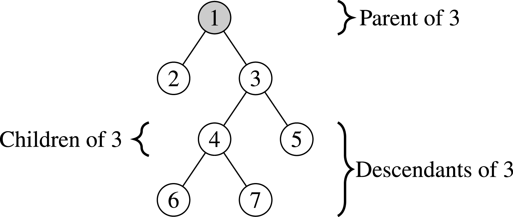
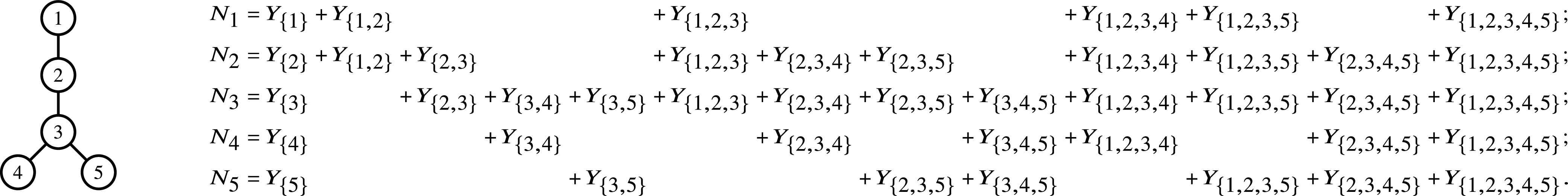


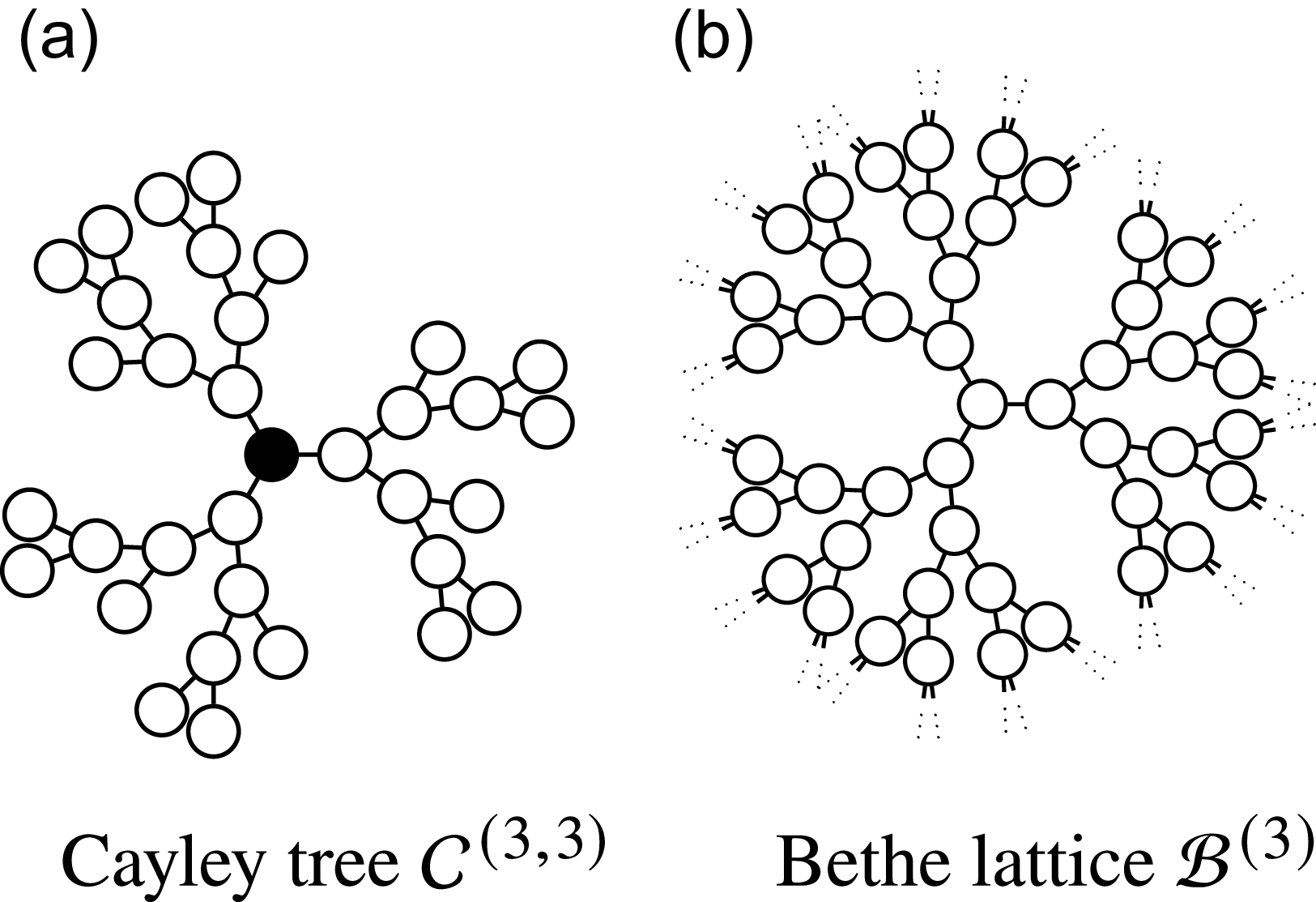
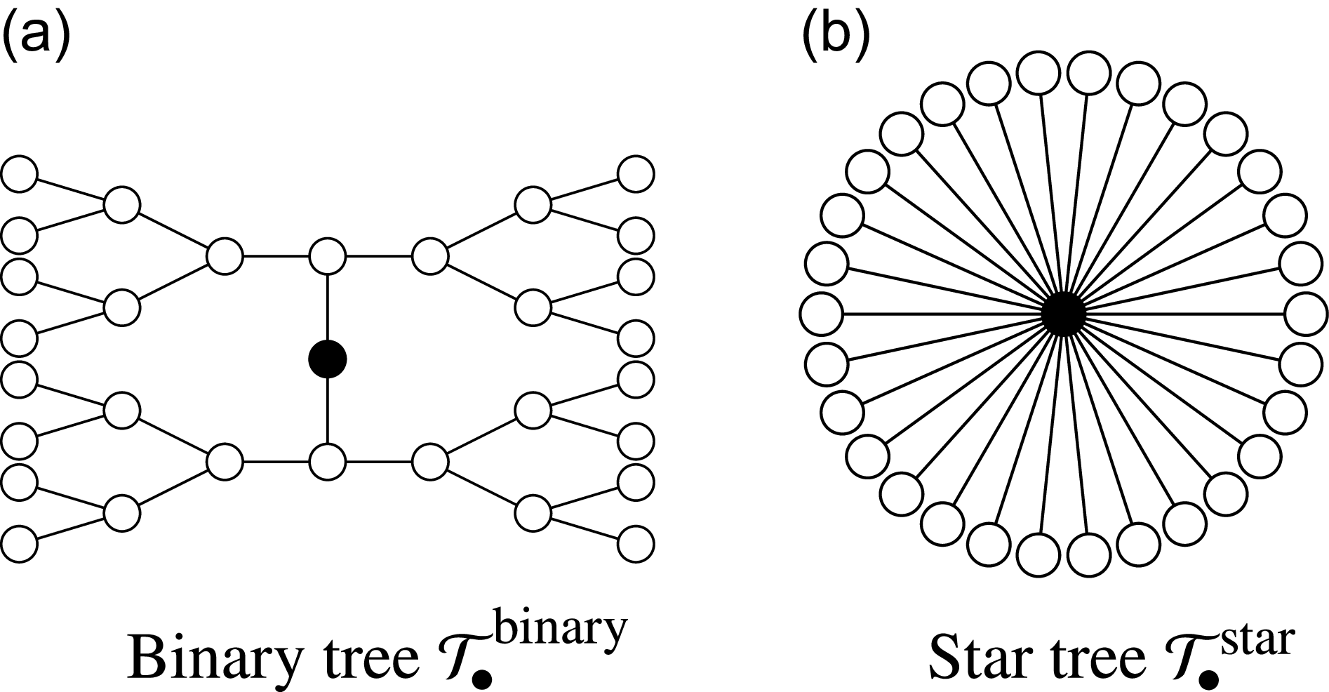
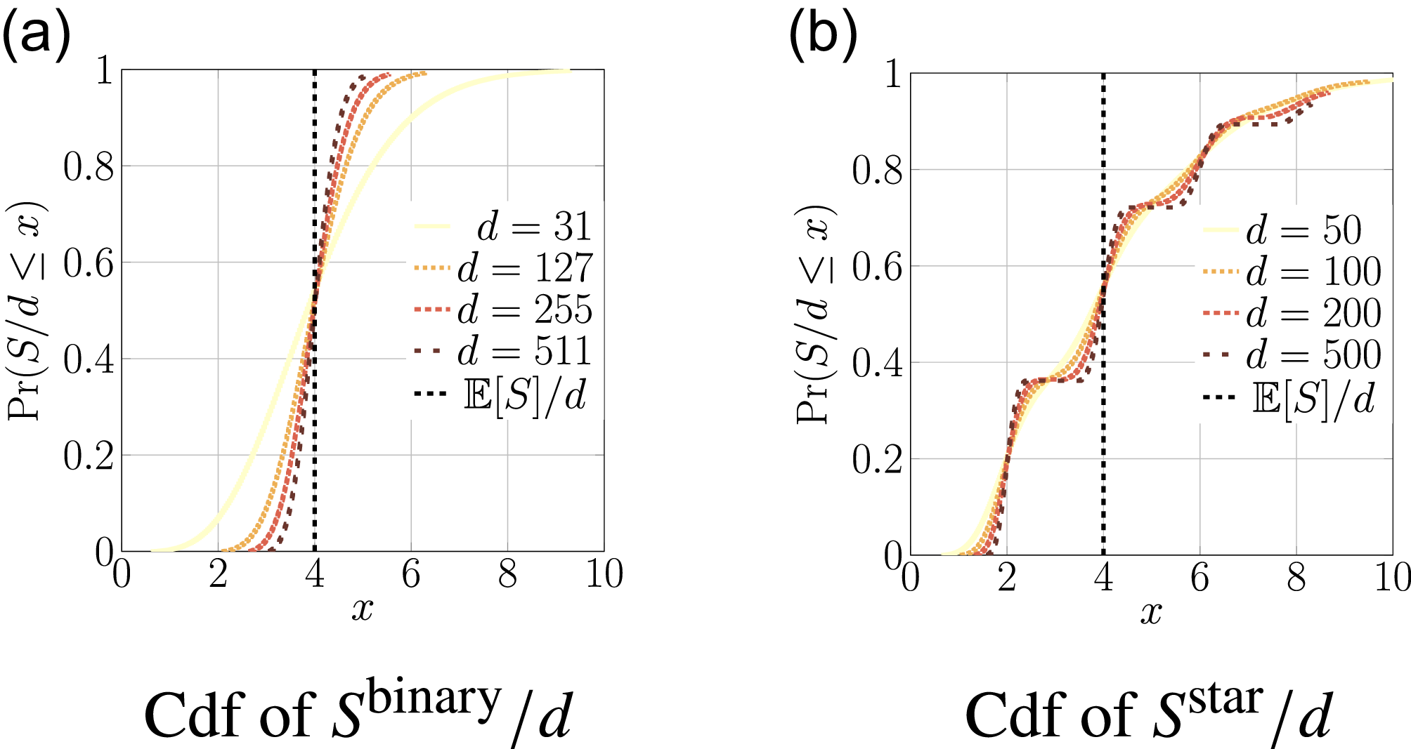

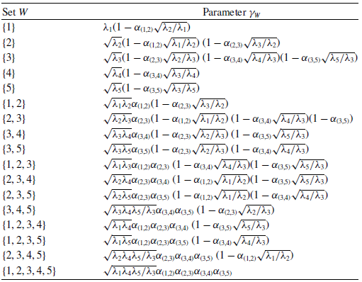


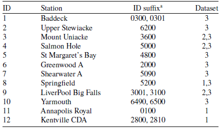
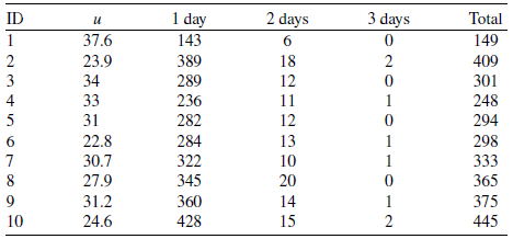
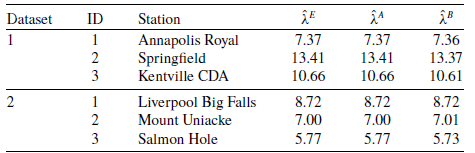
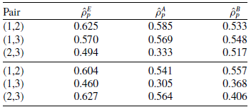
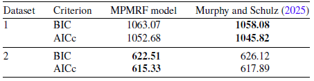
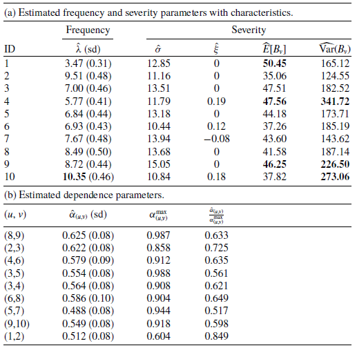


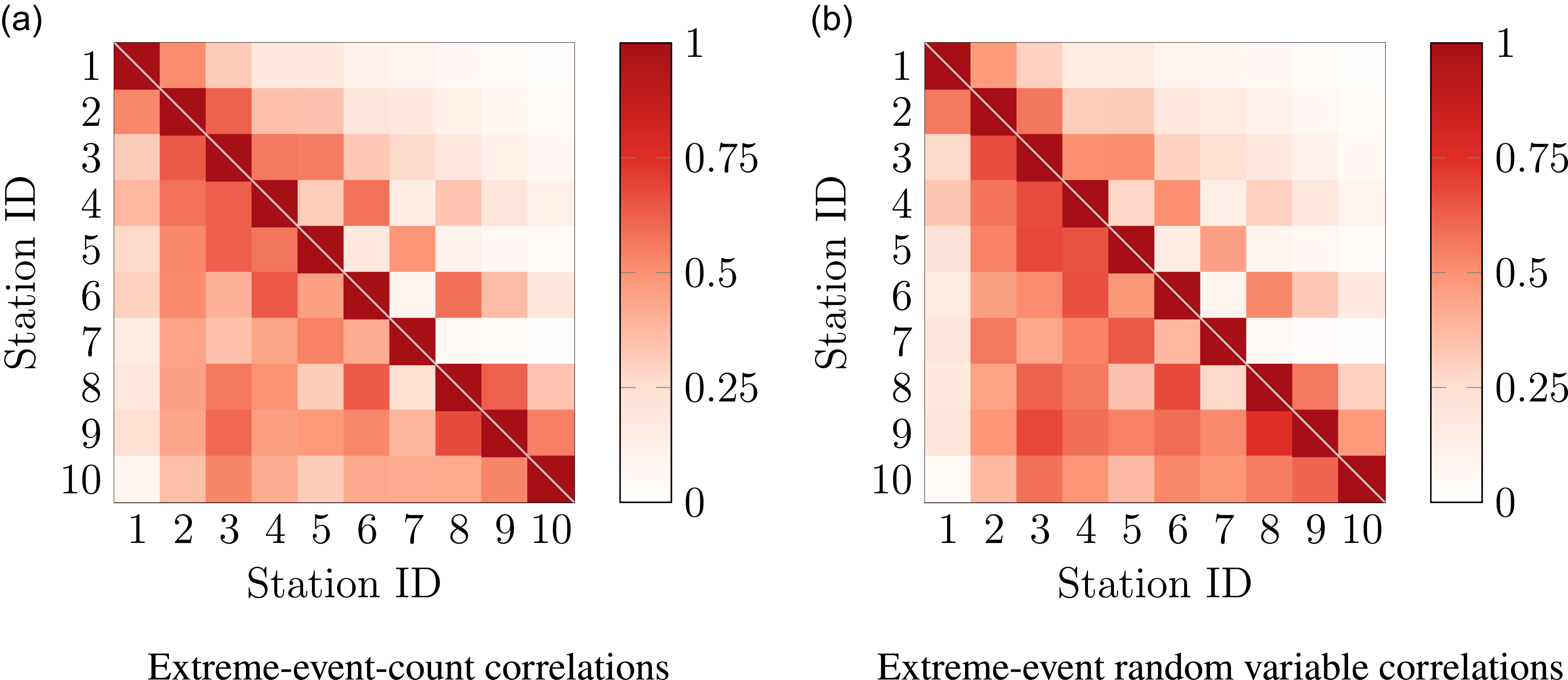
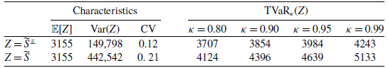


 Open access