

1 Introduction
In educational and psychological measurement, item response times (RTs), as a type of process data, offer valuable insights into examinees’ test-taking behaviors and performance (Lee & Chen, Reference Lee and Chen2011; Ratcliff & Kang, Reference Ratcliff and Kang2021; Schneider et al., Reference Schneider, Junghaenel, Meijer, Stone, Orriens, Jin, Zelinski, Lee, Hernandez and Kapteyn2023; Sinharay, Reference Sinharay2020; Ulitzsch et al., Reference Ulitzsch, von Davier and Pohl2020a, Reference Ulitzsch, von Davier and Pohl2020b, Reference Ulitzsch, Pohl, Khorramdel, Kroehne and von Davier2022; Wang & Xu, Reference Wang and Xu2015; Wang et al., Reference Wang, Zhang, Douglas and Culpepper2018). With the increasing prevalence of computerized testing, the routine collection of RTs has become more feasible, providing researchers with unprecedented opportunities to explore its psychometric properties and applications across diverse assessment settings.
A central methodological task is the development of appropriate statistical models for analyzing RTs. Early work (e.g., Entink, van der Linden, et al., Reference Entink, van der Linden and Fox2009; Rouder et al., Reference Rouder, Sun, Speckman, Lu and Zhou2003; van der Linden, Reference van der Linden2006) focused on modeling RTs independently of item responses, aiming to characterize their statistical properties and infer latent cognitive mechanisms. Several distributional models have been proposed in this context, including the log-normal model (van der Linden, Reference van der Linden2006), the Box–Cox normal model (Entink, van der Linden, et al., Reference Entink, van der Linden and Fox2009), the semiparametric model (Wang et al., Reference Wang, Fan, Chang and Douglas2013), and the shifted Weibull distribution (Rouder et al., Reference Rouder, Sun, Speckman, Lu and Zhou2003), among which the log-normal model has gained wide adoption due to its estimation simplicity and robust empirical performance (Sinharay & van Rijn, Reference Sinharay and van Rijn2020).
To better leverage RTs for psychological and educational measurement, it is crucial to propose the joint model for RTs and item responses. One of the most widely used frameworks is the hierarchical model (HM) proposed by van der Linden (Reference van der Linden2007), which specifies separate submodels for RTs and responses at the first level and captures their correlations at the person and item levels through a second-level structure. This framework focuses on the between-person relationship between ability and speed and has been extended in various directions to accommodate different testing contexts (Entink, Fox, et al., Reference Entink, Fox and van der Linden2009; Klein Entink et al., Reference Klein Entink, Kuhn, Hornke and Fox2009; Ulitzsch et al., Reference Ulitzsch, Pohl, Khorramdel, Kroehne and von Davier2022; Zhan, Jiao, & Liao, Reference Zhan, Jiao and Liao2018; Zhan, Jiao, Wang, et al., Reference Zhan, Jiao, Wang and Man2018). A key limitation of the HM, however, is its assumption of conditional independence between responses and RTs given the latent traits. Empirical studies have questioned this assumption, demonstrating residual dependence not fully explained by the correlation between latent traits (Bolsinova & Tijmstra, Reference Bolsinova and Tijmstra2019; Bolsinova, De Boeck, et al., Reference Bolsinova, De Boeck and Tijmstra2017; Meng et al., Reference Meng, Tao and Chang2015). To address this issue, various conditional joint models for item responses and RTs have been proposed.
One approach is modeling the joint distribution of RTs and responses as a bivariate distribution with a nonzero dependence parameter. For example, Ranger and Ortner (Reference Ranger and Ortner2012) proposed a conditional joint model that incorporates a covariance structure to capture local dependence between speed and accuracy. Extending this approach, Meng et al. (Reference Meng, Tao and Chang2015) allowed the conditional correlation to vary across both items and individuals, thereby improving the model’s flexibility in capturing person- and item-specific dependencies. Another widely used strategy factorizes the joint distribution into the product of a marginal distribution for RTs and a conditional distribution for responses given RTs. This approach provides greater modeling flexibility while maintaining interpretability. For instance, Bolsinova, De Boeck, et al. (Reference Bolsinova, De Boeck and Tijmstra2017) introduced a joint model that incorporates residual RTs into the item response model to account for unexplained dependence. Similarly, Bolsinova, Tijmstra, et al. (Reference Bolsinova, Tijmstra and Molenaar2017) proposed a joint modeling framework in which the conditional distribution of responses given RTs follows a two-parameter normal ogive (2PNO) model, with the intercept expressed as a linear function of log-transformed RTs. In contrast, Bolsinova and Tijmstra (Reference Bolsinova and Tijmstra2019) proposed another strategy by reversing the factorization direction. Specifically, they factorized the joint distribution into the product of a marginal distribution for responses and a conditional distribution for RTs given responses. This formulation allows for modeling RT heterogeneity as a function of response accuracy, explicitly distinguishing between correct and incorrect responses.
In addition, process-based approaches have emerged that seek to model both RTs and responses as outputs of an underlying cognitive process. These models integrate item response theory with decision-making models. For instance, diffusion IRT models embed a diffusion decision process within an IRT framework (Tuerlinckx & De Boeck, Reference Tuerlinckx and De Boeck2005) and were implemented through the diffIRT package (Molenaar et al., Reference Molenaar, Tuerlinckx and van der Maas2015b). Building on these works, Kang et al. (Reference Kang, De Boeck and Ratcliff2022) extended the diffusion IRT framework by allowing person- and item-level variability, thereby allowing the model to capture the conditional dependence between responses and RTs. Further, Kang, Jeon, et al. (Reference Kang, Jeon and Partchev2023) introduced a latent space diffusion IRT model in which both persons and items are embedded in a latent space to capture complex dependency between RTs and responses. These models depart from conventional statistical formulations and instead aim to recover the cognitive mechanisms driving observed RT and response patterns.
Despite these methodological advances, most existing joint models have been developed for dichotomous items, and research on polytomous items remains scarce. Molenaar et al. (Reference Molenaar, Tuerlinckx and van der Maas2015a, Reference Molenaar, Tuerlinckx and van der Maas2015c) demonstrated that, for graded response items, the HM can be reformulated as a generalized linear factor model when parameter dependence is ignored, enabling estimation using Mplus. These studies extended the applications of the HM and provided powerful and efficient computational tools for estimating joint models of item responses and RTs. Nevertheless, their work does not propose a dedicated joint modeling framework for graded-response or mixed-format assessments. More recently, Kang, Molenaar, et al. (Reference Kang, Molenaar and Ratcliff2023) proposed a process-based model for Likert-type items, but their framework is confined to non-cognitive assessments. Consequently, a fully specified joint model for graded responses and RTs in cognitive assessment is still lacking. This gap underscores the need for joint models that can accommodate these item formats and effectively capture the relationship between item responses and RTs.
In this study, drawing on the framework of Bolsinova and Tijmstra (Reference Bolsinova and Tijmstra2019), we develop a joint model for graded responses and RTs. The proposed approach develops a conditional RT model given item responses and integrates it with a marginal response model based on Samejima’s graded response model (GRM; Samejima, Reference Samejima1969). This integration yields a conditional joint model that captures the within-person relationship between item responses and RTs. We further extend this model into a hierarchical formulation that accommodates between-person relationship between ability and speed. A second major contribution of this work is the development of a stochastic approximation EM (SAEM) algorithm for computing the marginal maximum likelihood estimate (MMLE) of the proposed model. The proposed estimation procedure is capable of handling mixed-format assessments that contain both binary and graded items. Finally, the proposed model and estimation procedure are evaluated through two simulation studies and an empirical analysis, demonstrating their practical applicability and strong performance.
The remainder of the article is organized as follows. Section 2 introduces a joint modeling framework for graded item responses and RTs. Section 3 presents an SAEM algorithm for estimating the proposed model. Section 4 reports simulation studies evaluating parameter recovery and comparing the graded response–response time (GR–RT) model with the HM. Section 5 applies the proposed method to empirical data to demonstrate its practical utility. Finally, we conclude with a discussion of the findings and directions for future research.
2 Model and rationale
In this section, we present a joint modeling framework for graded item responses and RTs, beginning with an empirical example that illustrates the dependence between RTs and response categories. Building on these observations, we construct a conditional joint model and further extend it into a two-level hierarchical structure.
2.1 Empirical investigation of the relationship between RTs and response categories
In this empirical analysis, we examine the differences in RTs across students with varying graded responses, using data from the Programme for International Student Assessment (PISA) scientific literacy assessment. The dataset contains responses from 717 Spanish students to 10 items, including six dichotomous and four polytomous items.
Because RTs are typically modeled on the log scale, we analyze the logarithmic transformation of RTs. Substantial variation in mean log-RTs is observed across response categories. As shown in the left panel of Figure 1, for a four-category item (“DS643Q04R”), the mean log-RTs increases with response category, particularly from category 1 to 2. F tests confirm that these differences are statistically significant at the 0.05 level. This pattern suggests that responses in higher categories tend to be associated with longer RTs. However, part of this relationship may be driven by individual differences in speed. To account for this, we conducted a residual-based analysis.
Line charts of mean log–response times
$(\log t_{ij})$
 and mean residuals
$(\hat {\epsilon }_{ij})$
and mean residuals
$(\hat {\epsilon }_{ij})$
 across different response categories for item “DS643Q04R.”

Figure 1 Long description
The figure consists of two side-by-side line graphs with dashed blue lines and star-shaped markers.
Left Panel: Mean log t.
- The x-axis is labeled Item response with values 0, 1, 2, and 3.
- The y-axis is labeled Mean log t with values ranging from 3.8 to 4.6.
- The data shows a slight decrease from response 0 to 1, followed by a sharp linear increase to response 2, and a continued moderate increase to response 3.
Right Panel: Mean residuals epsilon-hat.
- The x-axis is labeled Item response with values 0, 1, 2, and 3.
- The y-axis is labeled Mean residuals (epsilon-hat) with values ranging from -0.2 to 0.2.
- The data shows a gradual increase from response 0 to 1, a steep increase to a peak at response 2, and a decrease back toward the zero line at response 3.
Specifically, we modeled the RT data using the log-normal model proposed by Klein Entink et al. (Reference Klein Entink, Kuhn, Hornke and Fox2009), which decomposes log-RT into item-level and person-level components. Let
$T_{ij}$
 denote the RT variable of test taker i on item j, with
$t_{ij}$
denote the RT variable of test taker i on item j, with
$t_{ij}$
 denoting its realization. This model is given by

where
$v_{i}\in \left ( -\infty ,+\infty \right )$
 is the latent speed trait for examinee i, and
$\beta _{j}\in \left ( -\infty ,+\infty \right )$
is the latent speed trait for examinee i, and
$\beta _{j}\in \left ( -\infty ,+\infty \right )$
 ,
$\varphi _{j}\in \left ( 0,+\infty \right )$
,
$\varphi _{j}\in \left ( 0,+\infty \right )$
 , and
$\sigma _{j}^2\in \left ( 0,+\infty \right )$
, and
$\sigma _{j}^2\in \left ( 0,+\infty \right )$
 denote the time intensity, speed discrimination, and the variance parameters for item j, respectively. After estimating the model, we obtained parameter estimates
$\hat {\beta }_j, \hat {\varphi }_j, \hat {\sigma }_j$
denote the time intensity, speed discrimination, and the variance parameters for item j, respectively. After estimating the model, we obtained parameter estimates
$\hat {\beta }_j, \hat {\varphi }_j, \hat {\sigma }_j$
 , and
$\hat {v}_i$
, and
$\hat {v}_i$
 , and computed residuals

which represent log-RTs adjusted for individual speed and item-level effects. These residuals allow for a reassessment of RT differences across response categories without confounding due to person or item variability.
The right panel of Figure 1 presents the mean residuals across response categories. Compared to the raw log-RTs, the residual pattern differs slightly, displaying a peak at category 2 followed by a decline. This indicates that part of the trend in raw log-RTs was attributable to individual speed differences. Nevertheless, an overall upward pattern remains, and F tests confirm that the differences in mean residuals across categories are remain statistically significant at the 0.05 level.
Overall, these findings indicate a clear relationship between RTs and response categories. To more adequately capture this relationship, we propose an RT model that explicitly incorporates category-specific effects, as described in the following section.
2.2 A joint model for graded responses and RTs
We begin by defining some notation. Let test takers be indexed by
$i=1,\ldots ,N$
 and items indexed by
$j=1,\ldots ,M$
and items indexed by
$j=1,\ldots ,M$
 . Let
$Y_{ij}$
. Let
$Y_{ij}$
 be the response variable of test taker i to item j, with
$y_{ij}$
be the response variable of test taker i to item j, with
$y_{ij}$
 representing its observed value. Without loss of generality, we assume
$y_{ij}=0,\ldots ,K_j-1$
representing its observed value. Without loss of generality, we assume
$y_{ij}=0,\ldots ,K_j-1$
 , where K
j
≥ 2 is the total number of response categories. Finally, let I
(⋅) denote the indicator function.
, where K
j
≥ 2 is the total number of response categories. Finally, let I
(⋅) denote the indicator function.
2.2.1 A conditional model for RTs given item responses
To capture the effect of the ordinal response Y
ij
on the RTs, we adopt a dummy coding approach. Specifically, we define a dummy variable vector as
$\mathbf {Z}_{Y_{ij}}$
 ,
,

Let
$\mathbf {z}_{y_{ij}}=(z_{ijk})_{1\leq k \leq K_{j}-1}$
 denote an observation of
$\mathbf {Z}_{Y_{ij}}$
denote an observation of
$\mathbf {Z}_{Y_{ij}}$
 . Under this encoding scheme, the relationship between y
ij
and
$\mathbf {z}_{y_{ij}}$
. Under this encoding scheme, the relationship between y
ij
and
$\mathbf {z}_{y_{ij}}$
 is given by

As noted above, the log-normal model is widely used for modeling RTs because it fits various data well and allows for reliable inference and future extensions. Therefore, we adopt the log-normal model in this study. To incorporate the influence of response categories on RTs, we extend the log-normal model by introducing category-specific parameters. The resulting conditional model for RTs given the observed response
$Y_{ij}=y_{ij}$
 is
is

Here,
$v_{i}$
 ,
$\beta _{j}$
,
$\beta _{j}$
 ,
$\varphi _{j}$
,
$\varphi _{j}$
 , and
$\sigma _{j}^2$
, and
$\sigma _{j}^2$
 are introduced above;
${\boldsymbol {\delta }}_{j}=(\delta _{j1},\delta _{j2},\ldots ,\delta _{j(K_{j}-1)})^\top $
are introduced above;
${\boldsymbol {\delta }}_{j}=(\delta _{j1},\delta _{j2},\ldots ,\delta _{j(K_{j}-1)})^\top $
 represents the item response-specific effect parameter for item j. The parameter
${\boldsymbol {\delta }}_{j}$
represents the item response-specific effect parameter for item j. The parameter
${\boldsymbol {\delta }}_{j}$
 quantifies the systematic differences in RTs associated with each response category.
2.2.2 Item response model
In this study, we employ the widely-used GRM proposed by Samejima (Reference Samejima1969) to model the ordered categorical response variable
$Y_{ij}$
 . Under the GRM, the probability that test taker i selects response category
$k~(k=0,\ldots ,K_j-1)$
. Under the GRM, the probability that test taker i selects response category
$k~(k=0,\ldots ,K_j-1)$
 for item j is given by

where

Here,
$\theta _i$
 denotes the latent ability of test taker i,
$a_j$
denotes the latent ability of test taker i,
$a_j$
 is the discrimination parameter,
$b_j$
is the discrimination parameter,
$b_j$
 is the difficulty parameter, and
${\pmb {\tau }}_j=(\tau _{j1},\ldots ,\tau _{j(K_j-1)})$
is the difficulty parameter, and
${\pmb {\tau }}_j=(\tau _{j1},\ldots ,\tau _{j(K_j-1)})$
 is the thresholds for item j, which correspond to the cut-off points between the response categories. The threshold parameters must satisfy the monotonicity condition
$\tau _{j1}<\tau _{j2}<\cdots <\tau _{j(K_{j}-1)}$
is the thresholds for item j, which correspond to the cut-off points between the response categories. The threshold parameters must satisfy the monotonicity condition
$\tau _{j1}<\tau _{j2}<\cdots <\tau _{j(K_{j}-1)}$
 . In addition, to ensure identifiability between
$b_j$
. In addition, to ensure identifiability between
$b_j$
 and
$\boldsymbol {\tau }$
and
$\boldsymbol {\tau }$
 , we impose the constraint:
$\sum _{k=1}^{K_j-1}\tau _{jk}=0 \quad \text {for } j=1,\dots ,M$
, we impose the constraint:
$\sum _{k=1}^{K_j-1}\tau _{jk}=0 \quad \text {for } j=1,\dots ,M$
 . The function
$F(\cdot )$
. The function
$F(\cdot )$
 refers to the cumulative distribution function (CDF) of either the logistic or the standard normal distribution. In this study, we use the standard normal CDF for convenience in developing the SAEM algorithm for model estimation.
Finally, based on the dummy variable vector
$\mathbf {Z}_{Y_{ij}}$
 in Equations (1) and (2), the probability mass function of the item response variable
$Y_{ij}$
in Equations (1) and (2), the probability mass function of the item response variable
$Y_{ij}$
 can be expressed as

2.2.3 A joint model for graded responses and RTs
Let
$\boldsymbol {\zeta }_i=(\theta _i,v_i)^\top $
 denote the latent trait vector of examinee i. For item j, let the GRM parameters be
$\boldsymbol {\eta }_j = (a_j, b_j, \boldsymbol {\tau }_j)^\top $
denote the latent trait vector of examinee i. For item j, let the GRM parameters be
$\boldsymbol {\eta }_j = (a_j, b_j, \boldsymbol {\tau }_j)^\top $
 , and let the RT model parameters be
$\boldsymbol {\alpha }_j = (\beta _j, \varphi _j, \boldsymbol {\delta }_j^\top , \sigma _j)^\top $
, and let the RT model parameters be
$\boldsymbol {\alpha }_j = (\beta _j, \varphi _j, \boldsymbol {\delta }_j^\top , \sigma _j)^\top $
 . The complete parameter vector for item j is given by
$\boldsymbol {\xi }_j = (\boldsymbol {\eta }_j^\top , \boldsymbol {\alpha }_j^\top )^\top $
. The complete parameter vector for item j is given by
$\boldsymbol {\xi }_j = (\boldsymbol {\eta }_j^\top , \boldsymbol {\alpha }_j^\top )^\top $
 .
.
Based on the conditional RT model in Equation (3) and the GRM in Equation (4), the conditional joint model of
$Y_{ij}$
 and
$T_{ij}$
and
$T_{ij}$
 given
${\boldsymbol {\zeta }}_i$
given
${\boldsymbol {\zeta }}_i$
 can be written as

where
$\phi (\cdot )$
 is the probability density function of the standard normal distribution.
Following the hierarchical modeling framework proposed by van der Linden (Reference van der Linden2007), the population-level distribution of the latent variables
${\boldsymbol {\zeta }}_i$
 is assumed to follow a bivariate normal distribution

where
$\boldsymbol {\mu }_p$
 and
$\boldsymbol {\Sigma }_{p}$
and
$\boldsymbol {\Sigma }_{p}$
 denote the mean vector and covariance matrix, respectively. For identification purposes, these parameters are typically specified as

Finally, based on Equations (5) and (6), a two-level hierarchical joint model for
$Y_{ij}$
 and
$T_{ij}$
and
$T_{ij}$
 is given by

In this article, the proposed joint model is referred to as the GR–RT model, as it accounts for both graded responses and response times. Notably, when
${\boldsymbol {\delta }}_{j}=\mathbf {0}$
 , the GR–RT model reduces to the basic HM framework proposed by Klein Entink et al. (Reference Klein Entink, Kuhn, Hornke and Fox2009) for graded scoring items, where responses and RTs are conditionally independent. Moreover, since binary scoring is a special case of graded scoring, the GR–RT model provides a unified framework for analyzing test data that include both dichotomous and polytomous items.
Remark 1. The proposed GR–RT model is not a direct extension of the heterogeneity model introduced by Bolsinova and Tijmstra (Reference Bolsinova and Tijmstra2019), primarily due to certain practical challenges. In their framework, heterogeneity between correct and incorrect responses is modeled through multiple aspects, including the slope parameters (
$\varphi _j$
 ), residual variance (
$\sigma _j^2$
), residual variance (
$\sigma _j^2$
 ), and the joint population distribution of
$\theta $
), and the joint population distribution of
$\theta $
 and v. For polytomous items, modeling different slope parameters and residual variances for each response category, along with different distributions of
$\theta $
and v. For polytomous items, modeling different slope parameters and residual variances for each response category, along with different distributions of
$\theta $
 and v, results in a highly complex model structure. This complexity introduces significant challenges: not only does it make parameter estimation more difficult, but it also reduces the overall credibility of the model due to increased uncertainty in the estimation process. Moreover, real-world data often exhibit sparsity in certain response categories, which magnifies the uncertainty and undermines the reliability of statistical inference. Given these practical challenges, the present study adopts a more parsimonious approach by modeling response category-specific heterogeneity solely through intercept terms. While this approach captures only one aspect of heterogeneity, it provides a robust, manageable framework for analyzing polytomous items in the presence of RT data, and it lays the groundwork for future extensions that could incorporate richer heterogeneity structures as the field advances.
The practical applicability of a measurement model depends on the feasibility of accurately estimating its parameters. The complex structure of the GR–RT model presents significant challenges for parameter estimation. Therefore, developing an effective computational method to estimate the parameters of the GR–RT model is a central focus of this study. In the following section, we present an SAEM algorithm designed to compute the MMLE of the GR–RT model.
3 Model estimation
This section presents an SAEM algorithm for estimating the GR–RT model. In Section 3.1, a data augmentation scheme is introduced for the GR–RT model. Building on this data augmentation, Section 3.2 presents an SAEM algorithm for computing the MMLE of the GR–RT model.
3.1 A data augmentation scheme for GR−RT model
Data augmentation is fundamental for developing the SAEM algorithm. Following Camilli and Geis (Reference Camilli and Geis2019), we introduce a latent response vector
${\mathbf {X}}_{ij}=(X_{ij1},\ldots ,X_{ij(K_j-1)})^\top $
 , where each
$X_{ijk}$
, where each
$X_{ijk}$
 follows a normal distribution:

Moreover, the relationship between the observed response
$Y_{ij}$
 and the latent response
$X_{ijk}$
and the latent response
$X_{ijk}$
 is defined as

To intuitively illustrate this relationship between
${\mathbf {X}}_{ij}$
 and
$Y_{ij}$
and
$Y_{ij}$
 , consider a four-category graded response item, where
$Y_{ij}\in \{0,1,2,3\}$
, consider a four-category graded response item, where
$Y_{ij}\in \{0,1,2,3\}$
 and
${\mathbf {X}}_{ij}=(X_{ij1}, X_{ij2}, X_{ij3})^\top $
and
${\mathbf {X}}_{ij}=(X_{ij1}, X_{ij2}, X_{ij3})^\top $
 . When
$Y_{ij}$
. When
$Y_{ij}$
 takes the values
$0, 1, 2$
takes the values
$0, 1, 2$
 , and
$3$
, and
$3$
 , the corresponding ranges of the elements of
${\mathbf {X}}_{ij}$
, the corresponding ranges of the elements of
${\mathbf {X}}_{ij}$
 are determined, as shown in Table 1.
Relationship between
$Y{}_{ij}$
 and
${\mathbf {X}}{}_{ij}$
and
${\mathbf {X}}{}_{ij}$
 for four-category graded response

Table 1 Long description
The table consists of 8 columns and 5 rows including the header.
* Header Row: The first two columns are unlabeled or serve as the index for Y sub i j. Columns 3 to 5 are labeled Y sub i j greater than or equal to 1, Y sub i j greater than or equal to 2, and Y sub i j greater than or equal to 3. Columns 6 to 8 are labeled X sub i j 1, X sub i j 2, and X sub i j 3.
* Row 1: Y sub i j equals 0. For this value, the conditions for Y sub i j greater than or equal to 1, 2, and 3 are all marked with a minus sign. Correspondingly, X sub i j 1, X sub i j 2, and X sub i j 3 are all marked as less than 0.
* Row 2: Y sub i j equals 1. The condition for Y sub i j greater than or equal to 1 is marked with a plus sign, while greater than or equal to 2 and 3 are marked with a minus sign. X sub i j 1 is greater than or equal to 0, while X sub i j 2 and X sub i j 3 are less than 0.
* Row 3: Y sub i j equals 2. The conditions for Y sub i j greater than or equal to 1 and 2 are marked with a plus sign, while greater than or equal to 3 is marked with a minus sign. X sub i j 1 and X sub i j 2 are greater than or equal to 0, while X sub i j 3 is less than 0.
* Row 4: Y sub i j equals 3. All conditions for Y sub i j greater than or equal to 1, 2, and 3 are marked with a plus sign. All binary indicators X sub i j 1, X sub i j 2, and X sub i j 3 are greater than or equal to 0.
A footer note specifies that a plus sign indicates the condition is satisfied and a minus sign indicates it is not satisfied.
Note:
$+$
 indicates the condition is satisfied and
$-$
indicates the condition is satisfied and
$-$
 indicates not satisfied.
We now define some notations. Let
$\mathbf {y}_{\cdot j}= \left (y_{1j},\ldots , y_{Nj}\right )^\top $
 ,
$\mathbf {t}_{\cdot j}= \left (t_{1j},\ldots , t_{Nj}\right )^\top $
,
$\mathbf {t}_{\cdot j}= \left (t_{1j},\ldots , t_{Nj}\right )^\top $
 , and
$\ln \mathbf {t}_{.j}=(\ln t_{1j}, \ln t_{2j}, \ldots ,\\ \ln t_{Nj})^\top $
, and
$\ln \mathbf {t}_{.j}=(\ln t_{1j}, \ln t_{2j}, \ldots ,\\ \ln t_{Nj})^\top $
 denote the observed response, RT and log-RT vectors of item j, respectively. The observed response and RT data for all items are denoted by
$\mathbf {y}=\left ( \mathbf {y}_{\cdot 1},\ldots ,\mathbf {y}_{\cdot M}\right )$
denote the observed response, RT and log-RT vectors of item j, respectively. The observed response and RT data for all items are denoted by
$\mathbf {y}=\left ( \mathbf {y}_{\cdot 1},\ldots ,\mathbf {y}_{\cdot M}\right )$
 and
$\mathbf {t}=\left ( \mathbf {t}_{\cdot 1},\ldots ,\mathbf {t}_{\cdot M}\right )$
and
$\mathbf {t}=\left ( \mathbf {t}_{\cdot 1},\ldots ,\mathbf {t}_{\cdot M}\right )$
 . Let
${\mathbf {X}}_{j}= ({\mathbf {X}}_{1j}, {\mathbf {X}}_{2j},\ldots ,{\mathbf {X}}_{Nj})$
. Let
${\mathbf {X}}_{j}= ({\mathbf {X}}_{1j}, {\mathbf {X}}_{2j},\ldots ,{\mathbf {X}}_{Nj})$
 denote the latent response matrix for item j. Let
$\mathbf {x}_{ij}=(x_{ij1},\ldots ,x_{ij(K_j-1)})^\top $
denote the latent response matrix for item j. Let
$\mathbf {x}_{ij}=(x_{ij1},\ldots ,x_{ij(K_j-1)})^\top $
 denote the realization of
${\mathbf {X}}_{ij}$
denote the realization of
${\mathbf {X}}_{ij}$
 , and
$\mathbf {x}_{j}= (\mathbf {x}_{1j}, \mathbf {x}_{2j},\ldots ,\mathbf {x}_{Nj})$
, and
$\mathbf {x}_{j}= (\mathbf {x}_{1j}, \mathbf {x}_{2j},\ldots ,\mathbf {x}_{Nj})$
 denote the realization of
${\mathbf {X}}_{j}$
denote the realization of
${\mathbf {X}}_{j}$
 . Let
$\boldsymbol {\theta } = (\theta _1, \dots , \theta _N)^\top $
. Let
$\boldsymbol {\theta } = (\theta _1, \dots , \theta _N)^\top $
 and
$\mathbf {v} = (v_1, \dots , v_N)^\top $
and
$\mathbf {v} = (v_1, \dots , v_N)^\top $
 denote the latent ability and speed vectors, respectively. The combined latent traits are represented as
$\boldsymbol {\zeta } = (\boldsymbol {\theta }, \mathbf {v})$
denote the latent ability and speed vectors, respectively. The combined latent traits are represented as
$\boldsymbol {\zeta } = (\boldsymbol {\theta }, \mathbf {v})$
 . The complete data for the test, including observed responses, RTs, latent responses, and latent traits, are denoted by
$\mathbf {u}=(\mathbf {y}, \mathbf {t},\mathbf {x}^\top , {\boldsymbol {\zeta }})$
. The complete data for the test, including observed responses, RTs, latent responses, and latent traits, are denoted by
$\mathbf {u}=(\mathbf {y}, \mathbf {t},\mathbf {x}^\top , {\boldsymbol {\zeta }})$
 , while the complete data for item j are denoted by
$\mathbf {u}_{.j}=(\mathbf {y}_{.j}, \mathbf {t}_{.j},\mathbf {x}_j^\top , {\boldsymbol {\zeta }})$
, while the complete data for item j are denoted by
$\mathbf {u}_{.j}=(\mathbf {y}_{.j}, \mathbf {t}_{.j},\mathbf {x}_j^\top , {\boldsymbol {\zeta }})$
 . Let
$\boldsymbol {\eta }=(\boldsymbol {\eta }_1,\ldots ,\boldsymbol {\eta }_M)$
. Let
$\boldsymbol {\eta }=(\boldsymbol {\eta }_1,\ldots ,\boldsymbol {\eta }_M)$
 be the collection of GRM parameters and
$\boldsymbol {\alpha }=(\boldsymbol {\alpha }_1,\ldots ,\boldsymbol {\alpha }_M)$
be the collection of GRM parameters and
$\boldsymbol {\alpha }=(\boldsymbol {\alpha }_1,\ldots ,\boldsymbol {\alpha }_M)$
 be the collection of RT model parameters. The collection of all item parameters in the GR–RT model, combining of
$\boldsymbol {\eta }$
be the collection of RT model parameters. The collection of all item parameters in the GR–RT model, combining of
$\boldsymbol {\eta }$
 and
${\boldsymbol {\alpha }}$
and
${\boldsymbol {\alpha }}$
 , is denoted by
$\boldsymbol {\xi }=(\boldsymbol {\xi }_1,\ldots ,\boldsymbol {\xi }_M)$
, is denoted by
$\boldsymbol {\xi }=(\boldsymbol {\xi }_1,\ldots ,\boldsymbol {\xi }_M)$
 . Let
$\boldsymbol {\Omega }=(\boldsymbol {\xi }, \sigma _{\theta v})$
. Let
$\boldsymbol {\Omega }=(\boldsymbol {\xi }, \sigma _{\theta v})$
 be the set of parameters to be estimated in the GR–RT model.
Based on Equations (7)–(9), we have

Further, the complete-data likelihood of
$\boldsymbol {\xi }_j$
 and
$\sigma _{\theta v}$
and
$\sigma _{\theta v}$
 can be expressed as

where


It can be observed that
$L(\mathbf {u}_{.j} \mid {\boldsymbol {\xi }}_{j}, \sigma _{\theta v})$
 is the product of three normal likelihoods, which places it within the exponential family. When the data likelihood takes the form of an exponential family (Barndorff-Nielsen, Reference Barndorff-Nielsen2014), the implementation of the EM algorithm and its extensions is simplified to working with sufficient statistics (Dempster et al., Reference Dempster, Laird and Rubin1977). Therefore, the exponential family structure of the complete data likelihood is particularly advantageous for developing an SAEM algorithm for the GR–RT model.
For brevity, the exponential family form of
$L(\mathbf {u}_{.j} \mid {\boldsymbol {\xi }}_{j}, \sigma _{\theta v})$
 is not given here; instead, we present only the sufficient statistics for
${\boldsymbol {\xi }}_{j}$
is not given here; instead, we present only the sufficient statistics for
${\boldsymbol {\xi }}_{j}$
 and
$\sigma _{\theta v}$
and
$\sigma _{\theta v}$
 .
.
Specifically, the sufficient statistics for
$\boldsymbol {\eta }_j$
 are
are

where
$\sum _{i=1}^N \mathbf {x}_{ij}=(\sum _{i=1}^N x_{ij1},\ldots ,\sum _{i=1}^N x_{ij(K_j-1)})^\top $
 .
.
The sufficient statistics for
$\boldsymbol {\alpha }_j$
 are
are

where

Finally, the sufficient statistics for
$\sigma _{\theta v}$
 are
are

3.2 An SAEM algorithm for the MMLE of GR–RT model
We begin by introducing the EM algorithm for computing the MMLE of the GR–RT model, followed by the proposal of the SAEM algorithm.
3.2.1 EM algorithm
With the introduction of
${\mathbf {X}}_{ij}$
 , the E-step of EM algorithm simplifies to working with sufficient statistics, and the M-step directly updates the estimate of
$\boldsymbol {\Omega }$
, the E-step of EM algorithm simplifies to working with sufficient statistics, and the M-step directly updates the estimate of
$\boldsymbol {\Omega }$
 using the updated values of these sufficient statistics. Below, we present the general procedure of the EM algorithm, with a detailed implementation provided in Appendix A of the Supplementary Material.
Let
$\boldsymbol {\Omega }^{0}=(\boldsymbol {\xi }_{1}^{0},\ldots , \boldsymbol {\xi }_{M}^{0}, \sigma _{\theta v}^{0})$
 be the initial values of
$\boldsymbol {\Omega }$
be the initial values of
$\boldsymbol {\Omega }$
 , and
$\boldsymbol {\Omega }^{r-1}=(\boldsymbol {\xi }_{1}^{r-1},\ldots , \boldsymbol {\xi }_{M}^{r-1}, \sigma _{\theta v}^{r-1})$
, and
$\boldsymbol {\Omega }^{r-1}=(\boldsymbol {\xi }_{1}^{r-1},\ldots , \boldsymbol {\xi }_{M}^{r-1}, \sigma _{\theta v}^{r-1})$
 denote the parameter values updated at the end of the
$(r-1)$
denote the parameter values updated at the end of the
$(r-1)$
 th iteration. The rth EM iteration consists of the following steps:
-
1. E-step: Compute the conditional expectations of the sufficient statistics $S_{\boldsymbol {\eta }_{j}}$
 ,
$S_{\boldsymbol {\alpha }_{j}}$
, and
$ S_{\sigma _{\theta v}}$
given
$\mathbf {y}$
,
$\mathbf {t}$
, and
$\boldsymbol {\Omega }^{r-1}$
: $$ \begin{align*} {s}_{\boldsymbol{\eta}_j}^{r}=E_{(\mathbf{x}_j, \boldsymbol{\theta})}(S_{\boldsymbol{\eta}_{j}}|\mathbf{y}, \mathbf{t},\boldsymbol{\Omega}^{r-1}), s_{\boldsymbol{\alpha}_j}^{r}=E_{\mathbf{v}}(S_{\boldsymbol{\alpha}_{j}}|\mathbf{y}, \mathbf{t},\boldsymbol{\Omega}^{r-1}), \quad \text{for } j=1,\ldots,M, \nonumber \end{align*} $$and
$$ \begin{align*} s_{\sigma_{\theta v}}^{r}=E_{\boldsymbol{\zeta}}(S_{\sigma_{\theta v}}|\mathbf{y}, \mathbf{t},\boldsymbol{\Omega}^{r-1}).\nonumber \end{align*} $$
,
$S_{\boldsymbol {\alpha }_{j}}$
, and
$ S_{\sigma _{\theta v}}$
given
$\mathbf {y}$
,
$\mathbf {t}$
, and
$\boldsymbol {\Omega }^{r-1}$
: $$ \begin{align*} {s}_{\boldsymbol{\eta}_j}^{r}=E_{(\mathbf{x}_j, \boldsymbol{\theta})}(S_{\boldsymbol{\eta}_{j}}|\mathbf{y}, \mathbf{t},\boldsymbol{\Omega}^{r-1}), s_{\boldsymbol{\alpha}_j}^{r}=E_{\mathbf{v}}(S_{\boldsymbol{\alpha}_{j}}|\mathbf{y}, \mathbf{t},\boldsymbol{\Omega}^{r-1}), \quad \text{for } j=1,\ldots,M, \nonumber \end{align*} $$and
$$ \begin{align*} s_{\sigma_{\theta v}}^{r}=E_{\boldsymbol{\zeta}}(S_{\sigma_{\theta v}}|\mathbf{y}, \mathbf{t},\boldsymbol{\Omega}^{r-1}).\nonumber \end{align*} $$
-
2. M-step: Update the parameter estimate of $\boldsymbol {\Omega }$
by $$ \begin{align*}\boldsymbol{\eta}^r_j=\hat{\boldsymbol{\eta}}_j(s_{\boldsymbol{\eta}_j}^{r}), \boldsymbol{\alpha}^r_j=\hat{\boldsymbol{\alpha}}_j(s_{\boldsymbol{\alpha}_j}^{r}),\text{for } j=1,\ldots,M,\end{align*} $$and
$$ \begin{align*}\sigma_{\theta v}^r=\hat{\sigma}_{\theta v}(s_{\sigma_{\theta v}}^{r}),\end{align*} $$
where the expressions of $\hat {\boldsymbol {\eta }}_j(s_{\boldsymbol {\eta }_j}^{r})$
,
$\hat {\boldsymbol {\alpha }}_j(s_{\boldsymbol {\alpha }_j}^{r})$
, and
$\hat {\sigma }_{\theta v}(s_{\sigma _{\theta v}}^{r})$
are provided in Equations (A10)–(A13) in the Supplementary Material.


While the M-step in the above EM iteration is straightforward and avoids the need for tedious optimization procedures, the E-step involves complex multidimensional integrals. To address this challenge, we propose an SAEM algorithm, inspired by existing studies (Camilli & Geis, Reference Camilli and Geis2019; Lavielle & Mbogning, Reference Lavielle and Mbogning2014; Meng & Xu, Reference Meng and Xu2023), which replaces the E-step computation with stochastic approximation, thereby reducing the computational burden.
3.2.2 A dimensionality reduction computation of
$E_{(\mathbf {x}_j, \boldsymbol {\theta })}(S_{\boldsymbol {\eta }_{j}} \mid \mathbf {y}, \mathbf {t}, \boldsymbol {\Omega }^{r-1})$

Using the law of total expectation (Kolmogorov, Reference Kolmogorov2018),

From Equation (14), the inner expectation
$E_{\mathbf {x}_{j}}(S_{\boldsymbol {\eta }_{j}} \mid \boldsymbol {\theta }, \mathbf {y}, \mathbf {t}, \boldsymbol {\Omega }^{r-1})$
 is given by

where

According to the relationship between
$X_{ijk}$
 and
$Y_{ij}$
and
$Y_{ij}$
 defined in Equation (9), the conditional distribution of
$X_{ijk}$
defined in Equation (9), the conditional distribution of
$X_{ijk}$
 given
$Y_{ij}=y_{ij}$
given
$Y_{ij}=y_{ij}$
 is given by

Further, it can be derived that the conditional expectation of
$X_{ijk}$
 given
$\boldsymbol {\theta }$
given
$\boldsymbol {\theta }$
 ,
$\mathbf {y}$
,
$\mathbf {y}$
 ,
$\mathbf {t}$
,
$\mathbf {t}$
 , and
$\boldsymbol {\Omega }^{r-1}$
, and
$\boldsymbol {\Omega }^{r-1}$
 is
is

Finally, by substituting the expression for
$E(X_{ijk} \mid \boldsymbol {\theta }, \mathbf {y}, \mathbf {t}, \boldsymbol {\Omega }^{r-1})$
 in Equation (19) into Equations (17) and (18), the closed form of
$E_{\mathbf {x}_{j}}(S_{\boldsymbol {\eta }_{j}} \mid \boldsymbol {\theta }, \mathbf {y}, \mathbf {t}, \boldsymbol {\Omega }^{r - 1})$
in Equation (19) into Equations (17) and (18), the closed form of
$E_{\mathbf {x}_{j}}(S_{\boldsymbol {\eta }_{j}} \mid \boldsymbol {\theta }, \mathbf {y}, \mathbf {t}, \boldsymbol {\Omega }^{r - 1})$
 is obtained. Let
$h_j^r({\boldsymbol {\theta }})=E_{\mathbf {x}_{j}}(S_{\boldsymbol {\eta }_{j}} \mid \boldsymbol {\theta }, \mathbf {y}, \mathbf {t}, \boldsymbol {\Omega }^{r-1})$
is obtained. Let
$h_j^r({\boldsymbol {\theta }})=E_{\mathbf {x}_{j}}(S_{\boldsymbol {\eta }_{j}} \mid \boldsymbol {\theta }, \mathbf {y}, \mathbf {t}, \boldsymbol {\Omega }^{r-1})$
 , then we have

This reduces the expectation of
$S_{\boldsymbol {\eta }_{j}}$
 with respect to
$\boldsymbol {\theta }$
with respect to
$\boldsymbol {\theta }$
 and
${\mathbf {X}}$
and
${\mathbf {X}}$
 to the expectation of
$h_j^r({\boldsymbol {\theta }})$
to the expectation of
$h_j^r({\boldsymbol {\theta }})$
 with respect to
$\boldsymbol {\theta }$
with respect to
$\boldsymbol {\theta }$
 , thereby achieving dimensionality reduction.
3.2.3 General framework of the SAEM algorithm
Based on the E-step in Equation (20), and following Delyon et al. (Reference Delyon, Lavielle and Moulines1999), the rth SAEM iteration consists of the following three steps:
-
1. S-step: Randomly sample $\boldsymbol {\zeta }_{i}^{l}=(\theta _i^l, v_i^l) (l=1,\ldots ,m_r)$
from
$f(\boldsymbol {\zeta }_{i}|\mathbf {y},\mathbf {t},\boldsymbol {\Omega }^{r-1})$
, for
$i=1,\ldots ,N$
. The detailed sampling procedure is given in Appendix B of the Supplementary Material. -
2. SA-step: Let $\boldsymbol {\theta }^l=(\theta _1^l,\ldots ,\theta _N^l)^\top $
and
$\mathbf {v}^l=(v_1^l,\ldots ,v_N^l)^\top $
. Using the generated
$\boldsymbol {\theta }^l$
and
$\mathbf {v}^l$
, compute
$S_{\boldsymbol {\alpha }_{j}}^{l}$
,
$S_{\sigma _{\theta v}}^{l}$
, and
$h_j^{r}(\boldsymbol {\theta }^{l})$
according to Equations 15–17, for
$l=1,\ldots ,m_r$
. The sufficient statistics are then updated as follows: $$ \begin{align*} s_{\boldsymbol{\eta}_j}^{r}&=s_{\boldsymbol{\eta}_j}^{r-1}+\gamma_r\left(\frac{\sum_{l=1}^{m_r}h_j^{r}(\boldsymbol{\theta}^{l})}{m_r}-s_{\boldsymbol{\eta}_j}^{r-1}\right),\nonumber\\ s_{\boldsymbol{\alpha}_j}^{r}&= s_{\boldsymbol{\alpha}_j}^{r-1}+\gamma_r\left(\frac{\sum_{l=1}^{m_r}S_{\boldsymbol{\alpha}_j}^{l}}{m_r}-s_{\boldsymbol{\alpha}_j}^{r-1}\right), \text{ for } j=1,\ldots,M, \nonumber \end{align*} $$and
$$ \begin{align*} s_{\sigma_{\theta v}}^{r}=s_{\sigma_{\theta v}}^{r-1}+\gamma_r\left(\frac{\sum_{l=1}^{m_r}S_{\sigma_{\theta v}}^{l}}{m_r}-s_{\sigma_{\theta v}}^{r-1}\right), \nonumber \end{align*} $$where $ \gamma _r>0$
,
$\sum _{r=1}^{+\infty }\gamma _r=+\infty $
and
$\sum _{r=1}^{+\infty }\gamma _r^2<+\infty $
.
-
3. M-Step: Compute
$$ \begin{align*}\boldsymbol{\eta}^r_j=\hat{\boldsymbol{\eta}}_j(s_{\boldsymbol{\eta}_j}^{r}),\boldsymbol{\alpha}^r_j=\hat{\boldsymbol{\alpha}}_j(s_{\boldsymbol{\alpha}_j}^{r}), \text{for } j=1,\ldots,M\end{align*} $$and
$$ \begin{align*}\sigma_{\theta v}^r=\hat{\sigma}_{\theta v}(s_{\sigma_{\theta v}}^{r}),\end{align*} $$according to Equations (A10)–(A13) in the Supplementary Material.


Remark 2. A crucial element of our SAEM algorithm is the use of
$h_j^r({\boldsymbol {\theta }})=E_{\mathbf {x}_{j}}(S_{\boldsymbol {\eta }_{j}} \mid \boldsymbol {\theta }, \mathbf {y}, \mathbf {t}, \boldsymbol {\Omega }^{r-1})$
 , which eliminates the need to sample
$\mathbf {x}_j$
, which eliminates the need to sample
$\mathbf {x}_j$
 during the S-step. This enhances computational efficiency and, more importantly, ensures that the estimates of
$\tau _{jk}^r (k=1,\ldots ,K_j-1)$
during the S-step. This enhances computational efficiency and, more importantly, ensures that the estimates of
$\tau _{jk}^r (k=1,\ldots ,K_j-1)$
 obtained in the M-step reliably preserve the desired ascending order:
$\tau ^r_{j1}<\tau ^r_{j2}<\cdots <\tau ^r_{j(K_j-1)}$
obtained in the M-step reliably preserve the desired ascending order:
$\tau ^r_{j1}<\tau ^r_{j2}<\cdots <\tau ^r_{j(K_j-1)}$
 . In contrast, if
$\mathbf {x}_j$
. In contrast, if
$\mathbf {x}_j$
 were randomly sampled during S-step, this order could be violated, as highlighted by Camilli and Geis (Reference Camilli and Geis2019). To illustrate this advantage, we first define
$\tilde {\tau }_{jk,l}^r$
were randomly sampled during S-step, this order could be violated, as highlighted by Camilli and Geis (Reference Camilli and Geis2019). To illustrate this advantage, we first define
$\tilde {\tau }_{jk,l}^r$
 according to Equation (A11) in the Supplementary Material, as follows:

where
$\mathbf {1}_{K_j-1}$
 denotes a
$(K_j-1)\times 1$
denotes a
$(K_j-1)\times 1$
 column vector with all entries equal to
$1$
column vector with all entries equal to
$1$
 . The term
$\left (\sum _{i=1}^{N}E({\mathbf {X}}_{ij}\mid \boldsymbol {\theta }^l, \mathbf {y},\mathbf {t},\boldsymbol {\Omega }^{r-1})\right )^\top \mathbf {1}_{K_j-1}$
. The term
$\left (\sum _{i=1}^{N}E({\mathbf {X}}_{ij}\mid \boldsymbol {\theta }^l, \mathbf {y},\mathbf {t},\boldsymbol {\Omega }^{r-1})\right )^\top \mathbf {1}_{K_j-1}$
 represents the summation of the elements within the vector
$\sum _{i=1}^{N}E({\mathbf {X}}_{ij}\mid \boldsymbol {\theta }^l, \mathbf {y},\mathbf {t},\boldsymbol {\Omega }^{r-1})$
represents the summation of the elements within the vector
$\sum _{i=1}^{N}E({\mathbf {X}}_{ij}\mid \boldsymbol {\theta }^l, \mathbf {y},\mathbf {t},\boldsymbol {\Omega }^{r-1})$
 . Using
$\tilde {\tau }_{jk,l}^r$
. Using
$\tilde {\tau }_{jk,l}^r$
 , the estimate
$\tau _{jk}^r$
, the estimate
$\tau _{jk}^r$
 in M-step of our SAEM can be equivalently computed as

Moreover, it can be easily shown that if the initial values of
$\boldsymbol {\tau }_j$
 satisfy
$\tau _{j1}^{0}<\cdots <\tau _{j(K_{j}-1)}^{0}$
satisfy
$\tau _{j1}^{0}<\cdots <\tau _{j(K_{j}-1)}^{0}$
 , the following order holds:

Thus, the order
$\tilde {\tau }_{j1,l}<\dots <\tilde {\tau }_{j(K_j-1),l}$
 is preserved, ensuring that
$\tau _{j1}^r<\dots <\tau _{j(K_j-1)}^r$
is preserved, ensuring that
$\tau _{j1}^r<\dots <\tau _{j(K_j-1)}^r$
 holds.
It is important to note that the SAEM procedure does not require the number of response categories
$K_j$
 to be the same across items, which makes it well-suited for estimating the GR–RT model with mixed-scoring items. In addition, because the HM is nested within the GR–RT model, the SAEM algorithm developed here can be directly applied to estimate the HM.
Large-scale assessments often employ matrix-sampling designs, leading to sparse response matrices with non-random missing data. This missingness is not a flaw in data collection but rather a natural consequence of the test booklet assignment process. To facilitate the flexible application of the GR–RT model in this context, we extended the SAEM algorithm to accommodate non-random missing data by introducing an indicator matrix
$\mathbf {D} = \{d_{ij}\}_{N \times M}$
 , where
$d_{ij} = 1$
, where
$d_{ij} = 1$
 denotes that item j is administered to respondent i, and
$d_{ij} = 0$
denotes that item j is administered to respondent i, and
$d_{ij} = 0$
 otherwise. This extension explicitly accounts for the non-ignorable missingness mechanism, allowing for valid parameter estimation under complex large-scale assessment designs. The detailed procedures of the extended SAEM algorithm are provided in Appendix C of the Supplementary Material.
3.2.4 Some specifications for implementing the SAEM algorithm
Initialization: Several studies, including Delyon et al. (Reference Delyon, Lavielle and Moulines1999), Lavielle and Mbogning (Reference Lavielle and Mbogning2014), and Meng and Xu (Reference Meng and Xu2023), have demonstrated that the SAEM algorithm is robust to the selection of initial values. To evaluate this robustness of our SAEM algorithm, we conducted a simulation study comparing parameter estimation performance with three different sets of initial values: a set of randomly selected values, a set of common values, and the true values of
$\boldsymbol {\Omega }$
 . The parameter recovery results across these different initial values were nearly identical, providing additional evidence of the SAEM algorithm’s robustness in terms of initial value selection. For the sake of conciseness, the details of this simulation study are not reported here. In both our simulation and empirical studies, we used the set of common values as the initial values.
The specifications of
$\gamma _r$
 : The choice of step size
$\gamma _r$
: The choice of step size
$\gamma _r$
 plays an important role in determining the convergence of the SAEM algorithm. Drawing on existing studies (Camilli & Geis, Reference Camilli and Geis2019; Lavielle & Mbogning, Reference Lavielle and Mbogning2014; Meng & Xu, Reference Meng and Xu2023), we adopt a two-stage step size sequence selection approach. Specifically, we set
$\gamma _r=1$
plays an important role in determining the convergence of the SAEM algorithm. Drawing on existing studies (Camilli & Geis, Reference Camilli and Geis2019; Lavielle & Mbogning, Reference Lavielle and Mbogning2014; Meng & Xu, Reference Meng and Xu2023), we adopt a two-stage step size sequence selection approach. Specifically, we set
$\gamma _r=1$
 during the initial R iterations (the first stage) and
$\gamma _r=\frac {1}{(r-R)^\kappa }$
during the initial R iterations (the first stage) and
$\gamma _r=\frac {1}{(r-R)^\kappa }$
 for
$r> R$
for
$r> R$
 (the second stage), where
$0.5 < \kappa \leq 1$
(the second stage), where
$0.5 < \kappa \leq 1$
 . In this study, we use
$\kappa = 1$
. In this study, we use
$\kappa = 1$
 . The step size sequence is thus expressed as
$\gamma _r = I_{(r \le R)} + I_{(r> R)}\,\frac {1}{r - R}$
. The step size sequence is thus expressed as
$\gamma _r = I_{(r \le R)} + I_{(r> R)}\,\frac {1}{r - R}$
 . In addition, through simulation studies, we verify that the convergence of the SAEM algorithm is ensured when
$R = 500$
. In addition, through simulation studies, we verify that the convergence of the SAEM algorithm is ensured when
$R = 500$
 .
.
The specifications of
$m_r$
 : Delyon et al. (Reference Delyon, Lavielle and Moulines1999) have demonstrated that the convergence of the SAEM algorithm is guaranteed with
$m_r = 1$
: Delyon et al. (Reference Delyon, Lavielle and Moulines1999) have demonstrated that the convergence of the SAEM algorithm is guaranteed with
$m_r = 1$
 . Notably, increasing
$m_r$
. Notably, increasing
$m_r$
 does not improve computational accuracy but instead adds to the computational burden. Therefore, in practical applications of the SAEM algorithm,
$m_r$
does not improve computational accuracy but instead adds to the computational burden. Therefore, in practical applications of the SAEM algorithm,
$m_r$
 is typically set to
$1$
is typically set to
$1$
 .
.
Convergence check: The convergence of the SAEM iteration is monitored using
$\Delta ^r=\|\boldsymbol {\Omega }^{r} - \boldsymbol {\Omega }^{r-1}\|_{\max }$
 . Here,
$\|\cdot \|_{\max }$
. Here,
$\|\cdot \|_{\max }$
 denotes the maximum of the absolute values within a vector. In this study, the SAEM iteration is recommended to terminate when
$\Delta ^r<10^{-4}$
denotes the maximum of the absolute values within a vector. In this study, the SAEM iteration is recommended to terminate when
$\Delta ^r<10^{-4}$
 or the maximum number of iterations exceeds 1,000.
4 Simulation studies
This section presents two simulation studies. Simulation Study 1 evaluated the parameter recovery of the GR–RT model and the HM within the MMLE framework using the SAEM algorithm, and also compared the results obtained from Mplus estimation. Simulation Study 2 compared the performance of the GR–RT model and the HM, and assessed the effectiveness of Akaike information criterion (AIC) and Bayesian information criterion (BIC) in selecting the correct model.
4.1 Simulation study 1
4.1.1 Design
This study investigated the performance of the proposed SAEM algorithm under mixed-format testing conditions that included both dichotomous and graded-response items. Without loss of generality, the graded items were specified to have four response categories. To assess the impact of item-type composition, five mixture proportions (MPs) of binary and graded-scoring items were considered, as shown in Table 2.
Five mixture proportion (MP) structures of four-category graded and binary items

Table 2 Long description
The table consists of six columns and three rows.
* The header row contains the column labels: M P 1, M P 2, M P 3, M P 4, and M P 5.
* The second row, labeled Four-category graded items, contains the following percentages: 100 percent, 70 percent, 50 percent, 30 percent, and 0 percent.
* The third row, labeled Binary items, contains the following percentages: 0 percent, 30 percent, 50 percent, 70 percent, and 100 percent.
The data shows an inverse relationship between the two item types across the five mixture proportions.
Since the sample size (N) and test length (M) are two important factors influencing the accuracy of the parameter estimation, this simulation considered three sample sizes (
$N = 500$
 , 1,000, and 2,000) and two test lengths (
$M = 20$
, 1,000, and 2,000) and two test lengths (
$M = 20$
 and 40). The three factors (sample size, test length, and MP) were crossed, resulting in
$ 3 \times 2 \times 5 = 30$
and 40). The three factors (sample size, test length, and MP) were crossed, resulting in
$ 3 \times 2 \times 5 = 30$
 simulation conditions. For each simulation condition, the item response and RT data were generated under two true models: the GR–RT model and the HM. The true parameter values were set as follows.
Let
$M_g$
 denote the number of graded-scored items, where
$j = 1, \dots , M_g$
denote the number of graded-scored items, where
$j = 1, \dots , M_g$
 indexes the graded items and
$j = M_g + 1, \dots , M$
indexes the graded items and
$j = M_g + 1, \dots , M$
 indexes the binary items. Let
$U(l_1,l_2)$
indexes the binary items. Let
$U(l_1,l_2)$
 denote the uniform distribution between
$l_1$
denote the uniform distribution between
$l_1$
 and
$l_2$
and
$l_2$
 , and
$LN(\mu ,\sigma ^2)$
, and
$LN(\mu ,\sigma ^2)$
 denote the log-normal distribution with parameters
$\mu $
denote the log-normal distribution with parameters
$\mu $
 and
$\sigma ^2$
and
$\sigma ^2$
 .
.
-
1. GR–RT model:
-
(a) Graded-scored items:
-
• GRM: For $j=1, \dots , M_g$
, the discrimination parameter
$a_j$
was generated from a uniform distribution,
$a_j \sim U(0.5,2.5)$
, allowing for moderate to high discrimination. The location parameter
$b_j$
was generated from a standard normal distribution,
$b_j\sim N(0,1)$
, to center the items on the ability scale. These specifications follow previous studies (e.g., Zhang & Chen, Reference Zhang and Chen2024; Wang & Xu, Reference Wang and Xu2015; Meng & Xu, Reference Meng and Xu2023). The threshold parameters
$\tau _{j1}, \tau _{j2}$
, and
$\tau _{j3}$
were generated as follows:
$\tau _{j1} \sim U(-1,-0.3)$
,
$\tau _{j2} \sim U(-0.25,0.25)$
, and
$\tau _{j3}=-\tau _{j1}-\tau _{j2}$
, such as
$\sum _{k=1}^{3}\tau _{jk}=0$
. These specifications based on empirical results from the data of one of the test booklets of the PISA 2022 science literacy assessment. -
• Log-normal RT model: For $j=1, \dots , M_g$
,
$\beta _j \sim U(3,5)$
,
${\boldsymbol {\delta }}_j \sim U(-1,1)$
,
$\sigma _j \sim U(0.3,0.7)$
, and
$\varphi _j\sim LN(0,0.5)$
. These specifications based on empirical results from the data of one of the test booklets of the PISA 2022 science literacy assessment.
-
-
(b) Binary-scored items:
-
• For $j=M_g+1,\dots , M$
, the true values of
$a_j$
,
$b_j$
,
$\sigma _j$
,
$\varphi _j$
,
$\beta _j$
, and
${\boldsymbol {\delta }}_j$
were generated in the same way as the parameters for the graded-scored items described in (a). Note that there is no
$\boldsymbol {\tau }$
-parameter, since the GRM is reduced to the 2PNO model.
-
-
-
2. Hierarchical model:
-
• The true values for the parameters in the GRM and log-normal RT models were generated in the same manner as for GR–RT model. Note that there is no $\boldsymbol {\delta }$
-parameter in the HM.
-
-
3. To account for a diverse range of correlations between ability and speed, the correlation coefficient $\sigma _{\theta v}$
was drawn from a uniform distribution,
$\sigma _{\theta v} \sim U(-1,1)$
, for each simulation condition. Given
$\sigma _{\theta v}$
, the person parameters were then sampled from the following bivariate normal distribution: $$ \begin{align*}(\theta_i,v_i)^T\sim N_2\left(\begin{pmatrix} 0 \\ 0 \end{pmatrix},\begin{pmatrix} 1 & \sigma_{\theta v}\\ \sigma_{\theta v} & 1 \end{pmatrix}\right),\end{align*} $$for $i = 1,\ldots ,N$
.


As noted by previous studies (Molenaar et al., Reference Molenaar, Tuerlinckx and van der Maas2015a, Reference Molenaar, Tuerlinckx and van der Maas2015c), the HM can be estimated using Mplus. Following the reviewers’ suggestion, we successfully implemented Mplus to estimate the GR–RT model. Thus, in this simulation, Mplus was used as a comparison tool to evaluate the performance of our proposed method. The Mplus code used for this purpose is provided in Appendix D of the Supplementary Material.
A total of 100 test datasets were generated for each of the two true models across all 30 testing scenarios. The GR–RT and HM models were fitted to their respective simulated data using both the SAEM algorithm and Mplus. Parameter estimation accuracy was assessed using the root mean square error (RMSE) and absolute bias (ABias), both computed as averages over 100 replications and all items. Taking the “a-parameter” as an example, we denote
$\hat {a}_{jg}$
 as the estimate of
$a_j$
as the estimate of
$a_j$
 obtained from the gth replication. The RMSE and ABias for the a-parameter were calculated as follows:

The computing time of both the SAEM algorithm and Mplus was also recorded for all simulation conditions to evaluate computational efficiency.
4.1.2 Results
The RMSE and ABias values for the SAEM estimation of the GR–RT model are presented in Tables 3 and 4. From these results, the following trends can be observed. First, both the RMSE and ABias for GR–RT model remain consistently small across all conditions. For example, the largest RMSE of the parameters is less than 0.2, and the ABias values are generally below 0.1. As the sample size increases, the RMSE and ABias values significantly decrease. In the case of
$N=2,000$
 , the RMSE values are smaller than 0.09, and the ABias values are nearly 0. These results demonstrate that increasing the sample size greatly improves the accuracy of parameter recovery and results in more unbiased estimators.
RMSE (ABias) of the estimates of GR–RT model, under three sample sizes (
$N=500$
 , 1,000, and 2,000) and five mixture proportions (MPs) of items (MP1, MP2, MP3, MP4, and MP5)

Table 3 Long description
The table is organized by sample size N (500, 1,000, and 2,000) and five mixture proportions (M P 1 through M P 5). Columns represent parameters: a, b, tau, sigma, varphi, beta, delta, and sigma sub theta v. Values are presented as R M S E with A Bias in parentheses.
* For N = 500:
- M P 1 (100% graded): a is 0.187 (0.110), b is 0.099 (0.045), tau is 0.051 (0.006).
- M P 5 (100% binary): a is 0.161 (0.066), b is 0.115 (0.059), tau is not applicable.
* For N = 1,000:
- M P 1 (100% graded): a is 0.145 (0.102), b is 0.062 (0.008), tau is 0.036 (0.004).
- M P 5 (100% binary): a is 0.103 (0.015), b is 0.102 (0.077).
* For N = 2,000:
- M P 1 (100% graded): a is 0.072 (0.029), b is 0.043 (0.009), tau is 0.025 (0.002).
- M P 5 (100% binary): a is 0.073 (0.014), b is 0.046 (0.006).
General trends show that as sample size N increases from 500 to 2,000, the R M S E values for most parameters decrease, indicating improved estimate precision. Binary item types consistently show no values for the tau parameter.
Note: The test length is
$M=20$
 . MP1: Four-category graded items (100%), binary items (0%); MP2: Four-category graded items (70%), binary items (30%); MP3: Four-category graded items (50%), binary items (50%); MP4: Four-category graded items (30%), binary items (70%); and MP5: Four-category graded items (0%), binary items (100%).
RMSE (ABias) of the estimates of GR–RT model, under three sample sizes (
$N=500$
 , 1,000, and 2,000) and five mixture proportions (MPs) of items (MP1, MP2, MP3, MP4, and MP5)

Table 4 Long description
The table is organized into three main sections based on sample size N: 500, 1,000, and 2,000. Each section is further divided by Mixture Proportions M P 1 through M P 5 and item types graded or binary. The columns represent parameters: a, b, tau, sigma, varphi, beta, delta, and sigma sub theta v. Values are presented as R M S E with A Bias in parentheses.
* For N = 500:
- M P 1 graded: a is 0.152 0.097, b is 0.099 0.059, tau is 0.049 0.005.
- M P 5 binary: a is 0.149 0.021, b is 0.119 0.060, delta is 0.055 0.005.
* For N = 1,000:
- M P 1 graded: a is 0.119 0.074, b is 0.059 0.007, tau is 0.036 0.003.
- M P 5 binary: a is 0.104 0.016, b is 0.072 0.017, delta is 0.042 0.003.
* For N = 2,000:
- M P 1 graded: a is 0.070 0.030, b is 0.051 0.029, tau is 0.025 0.002.
- M P 5 binary: a is 0.072 0.007, b is 0.058 0.029, delta is 0.028 0.002.
General trends show that as sample size N increases from 500 to 2,000, the R M S E and A Bias values generally decrease across all parameters. Binary items consistently lack a value for the tau parameter.
Note: The test length is
$M=40$
 . MP1: Four-category graded items (100%), binary items (0%); MP2: Four-category graded items (70%), binary items (30%); MP3: Four-category graded items (50%), binary items (50%); MP4: Four-category graded items (30%), binary items (70%); and MP5: Four-category graded items (0%), binary items (100%).
Second, across different proportions of four-category items and binary items, both the RMSE and ABias show only small differences, with no substantial increases in either under any test condition. This indicates that for estimating the GR–RT model, the performance of the SAEM algorithm is robust to the mixing of items in the test. Additionally, the RMSE and ABias are robust with regard to test length (M), which is expected, as the MMLE is theoretically independent of the test length.
Finally, both the RMSE and ABias for the RT model are smaller than those for the IRT model, indicating superior estimation accuracy. This is likely due to the linear nature of the RT model and the continuous nature of RT data, which allow for more precise parameter estimation compared to the discrete response data modeled by the IRT model.
The RMSE and ABias values for the SAEM estimation of the HM are reported in Tables 5 and 6. It is evident that these results follow similar trends to those for GR–RT model. Furthermore, both the RMSE and ABias are slightly smaller for HM, which is expected given that HM is a simpler model. Overall, our SAEM algorithm demonstrates effectiveness in estimating the HM. It provides a reliable approach for HM estimation and can be applied to estimate models in the context of graded-score items.
RMSE (ABias) of the estimates of HM, under three sample sizes (
$N=500$
 , 1,000, and 2,000) and five mixture proportions (MPs) of items (MP1, MP2, MP3, MP4, and MP5)

Table 5 Long description
The table consists of 10 columns: N, M Ps, Item types, a, b, tau, sigma, varphi, beta, and sigma sub bold theta bold v. Values are presented as R M S E with A Bias in parentheses.
For N = 500:
* M P 1 (100% graded): a = 0.151 (0.046), b = 0.118 (0.080), tau = 0.056 (0.005), sigma = 0.019 (0.002).
* M P 2 (70% graded, 30% binary): Graded items show a = 0.137 (0.015); Binary items show a = 0.127 (0.017).
* M P 3 (50% graded, 50% binary): Graded items show a = 0.140 (0.023); Binary items show a = 0.152 (0.015).
* M P 4 (30% graded, 70% binary): Graded items show a = 0.159 (0.051); Binary items show a = 0.165 (0.033).
* M P 5 (100% binary): a = 0.180 (0.041), b = 0.194 (0.130), sigma = 0.021 (0.001).
For N = 1,000:
* M P 1 (graded): a = 0.129 (0.090), b = 0.068 (0.032).
* M P 2: Graded a = 0.098 (0.015); Binary a = 0.088 (0.009).
* M P 5 (binary): a = 0.119 (0.029), b = 0.091 (0.014).
For N = 2,000:
* M P 1 (graded): a = 0.096 (0.065), b = 0.043 (0.012).
* M P 2: Graded a = 0.069 (0.020); Binary a = 0.064 (0.020).
* M P 5 (binary): a = 0.074 (0.013), b = 0.070 (0.035).
General trend: As sample size N increases from 500 to 2,000, the R M S E and A Bias values generally decrease across all parameters. Tau values are only provided for graded items.
Note: The test length is
$M=20$
 . MP1: Four-category graded items (100%), binary items (0%); MP2: Four-category graded items (70%), binary items (30%); MP3: Four-category graded items (50%), binary items (50%); MP4: Four-category graded items (30%), binary items (70%); and MP5: Four-category graded items (0%), binary items (100%).
RMSE (ABias) of the estimates of HM, under three sample sizes (
$N=500$
 , 1,000, and 2,000) and five mixture proportions (MPs) of items (MP1, MP2, MP3, MP4, and MP5)

Table 6 Long description
The table presents data for sample sizes N equals 500, 1,000, and 2,000. The columns include N, MPs (M P 1 to M P 5), Item types (graded or binary), and parameters a, b, tau, sigma, varphi, beta, and sigma sub theta v. Values are formatted as R M S E (A Bias).
* For N equals 500:
- M P 1 (100% graded): a is 0.146(0.068), b is 0.183(0.156), tau is 0.057(0.007).
- M P 2 (70% graded, 30% binary): Graded a is 0.125(0.036); Binary a is 0.156(0.030).
- M P 5 (100% binary): a is 0.154(0.029), b is 0.180(0.132), tau is not applicable.
* For N equals 1,000:
- M P 1: a is 0.094(0.022), b is 0.076(0.042).
- M P 3 (50% graded, 50% binary): Graded a is 0.109(0.050); Binary a is 0.108(0.033).
- M P 5: a is 0.117(0.038), b is 0.085(0.028).
* For N equals 2,000:
- M P 1: a is 0.067(0.019), b is 0.049(0.021).
- M P 4 (30% graded, 70% binary): Graded a is 0.095(0.070); Binary a is 0.094(0.059).
- M P 5: a is 0.077(0.013), b is 0.058(0.020).
General trend: R M S E and A Bias values generally decrease as the sample size N increases from 500 to 2,000 across all mixture proportions.
Note: The test length is
$M=40$
 . MP1: Four-category graded items (100%), binary items (0%); MP2: Four-category graded items (70%), binary items (30%); MP3: Four-category graded items (50%), binary items (50%); MP4: Four-category graded items (30%), binary items (70%); and MP5: Four-category graded items (0%), binary items (100%).
Under both the GR–RT and HM models, the RMSE and ABias values of
$\sigma _{\theta v}$
 are very small (all below 0.12). However, unlike the other parameters, neither index exhibits a clear decreasing trend as the sample size increases. This is due to the simulation design, in which the true values of
$\sigma _{\theta v}$
are very small (all below 0.12). However, unlike the other parameters, neither index exhibits a clear decreasing trend as the sample size increases. This is due to the simulation design, in which the true values of
$\sigma _{\theta v}$
 were randomly drawn from
$U(-1,1)$
were randomly drawn from
$U(-1,1)$
 in each simulation condition. As a result, different sample sizes correspond to different underlying true values, which can obscure the expected improvement in estimation accuracy with increasing sample size.
The computing time of the SAEM algorithm is displayed using boxplots, please see Figure 2. The top two figures present results for GR–RT model, while the bottom figures show results for HM. It can be observed that as the sample size increases, the computing time also increases. However, the maximum time required for a single run does not exceed 22 seconds, indicating that the SAEM algorithm demonstrates high computational efficiency. Additionally, the computing time for
$M = 40$
 is slightly greater than that for
$M = 20$
is slightly greater than that for
$M = 20$
 , and the computing time for GR–RT model is slightly longer than that for HM under the same simulation conditions. These phenomena are expected, as a larger sample size, longer test length, and the higher model complexity of GR–RT model result in increased computational cost.
Boxplots of computing time for GR–RT model (top row) and HM (bottom row), across varying sample sizes of
$N=500$
 , 1,000, and 2,000 and test lengths of
$M=20$
, 1,000, and 2,000 and test lengths of
$M=20$
 and 40 over 100 replications.

Figure 2 Long description
The figure consists of four panels arranged in a two-by-two grid. The top row shows results for the G R dash R T model, and the bottom row shows results for the H M model. Each panel has a y-axis labeled Computing Time in seconds, ranging from 0 to 20, and an x-axis with three categories for sample size N equals 500, N equals 1,000, and N equals 2,000.
* Top-left panel: G R dash R T model with Test Length M equals 20. Computing time increases with N. At N equals 500, the median is approximately 5. At N equals 1,000, the median is approximately 8. At N equals 2,000, the median is approximately 15.
* Top-right panel: G R dash R T model with Test Length M equals 40. Computing time shows a steeper increase. At N equals 500, the median is approximately 6. At N equals 1,000, the median is approximately 11. At N equals 2,000, the median is approximately 19.
* Bottom-left panel: H M model with Test Length M equals 20. Computing time is lower than G R dash R T. At N equals 500, the median is approximately 3. At N equals 1,000, the median is approximately 5. At N equals 2,000, the median is approximately 9.
* Bottom-right panel: H M model with Test Length M equals 40. Computing time increases with N. At N equals 500, the median is approximately 4. At N equals 1,000, the median is approximately 6. At N equals 2,000, the median is approximately 11.
Across all panels, the variance in computing time, indicated by the height of the blue boxes and whiskers, increases as the sample size N increases.
Due to space limitations, the results obtained from Mplus are provided in Appendix D of the Supplementary Material. The RMSE and ABias values for the GR–RT and HM parameter estimates using Mplus are summarized in Tables D1–D4 in the Supplementary Material. As shown, the RMSE and ABias values for certain parameters (e.g., a and b) are significantly larger, with some conditions producing values exceeding 10. These inflated values likely reflect instability in Mplus computations, particularly when the test includes mixed-format items, leading to extreme parameter estimates for both the GR–RT and HM models.
As shown in Figure D1 in the Supplementary Material, the computing time of Mplus remains reasonable when both N and M are small, slightly exceeding that of the SAEM algorithm under the same conditions. However, as sample size and test length increase, the computing time grows substantially. For instance, when
$N=2,000$
 and
$M=40$
and
$M=40$
 , a single run of Mplus exceeded 1,000 seconds for the GR–RT model and 700 seconds for the HM, indicating a significant computational burden.
4.2 Simulation study 2
The design and results are presented in Appendix E of the Supplementary Material; here, we briefly summarize the main findings.
The simulation results show that the GR–RT model generally outperforms the HM when the conditional independence assumption is violated (
${\boldsymbol {\delta }} \neq 0$
 ). Specifically, the GR–RT model produces lower RMSEs with fewer outliers, and its estimates of
$\sigma _{\theta v}$
). Specifically, the GR–RT model produces lower RMSEs with fewer outliers, and its estimates of
$\sigma _{\theta v}$
 are more closely centered around the true values. In contrast, the HM tends to underestimate
$\sigma _{\theta v}$
are more closely centered around the true values. In contrast, the HM tends to underestimate
$\sigma _{\theta v}$
 and yields unstable estimates under these conditions.
When
${\boldsymbol {\delta }} = 0$
 , where the HM is the true data-generating model, both models achieve similar accuracy. The HM demonstrates excellent parameter recovery, and the GR–RT model also maintains high accuracy, illustrating its robustness and adaptability across different data structures.
Both models show decreasing RMSEs with increasing sample size, reflecting consistency. However, under
${\boldsymbol {\delta }} \neq 0$
 , the HM continues to produce extreme estimates, indicating sensitivity to violations of conditional independence. Estimation stability for both models is also affected by the true value of
$\sigma _{\theta v}$
, the HM continues to produce extreme estimates, indicating sensitivity to violations of conditional independence. Estimation stability for both models is also affected by the true value of
$\sigma _{\theta v}$
 , with higher values associated with more stable estimates.
In summary, the GR–RT model provides accurate and stable parameter estimates when residual dependencies exist and remains robust when conditional independence holds. This makes it a flexible and reliable alternative to the HM across a range of testing scenarios.
Finally, we evaluated the performance of AIC and BIC in selecting true data-generating model. Both criteria consistently identified the true data-generating model as the best-fitting model across all 27 simulation conditions. These results highlight the high accuracy of AIC and BIC as model selection criteria in comparing the GR–RT model and the HM.
5 Empirical study
In this section, we present an empirical study conducted to evaluate the performance of the proposed GR–RT model using a mathematics dataset from PISA 2022.
5.1 Data and analysis design
PISA, conducted by the Organization for Economic Co-operation and Development (OECD), assesses the skills and knowledge of 15-year-old students in mathematics, reading, and science every three years across multiple countries. In this study, we focused on the mathematics assessment, as it was the primary focus of PISA 2022 and included a relatively high proportion of polytomous items.
The PISA 2022 mathematics assessment employed three testing formats: computer-based linear testing, computer-based multistage adaptive testing, and paper-based assessment. In this study, we analyzed data from the computer-based linear format, because the GR–RT model assumes a fixed test structure and is therefore not applicable to multistage adaptive testing. To align with the characteristics of large-scale assessments, which involve a large number of examinees and a wide range of items, we selected four test forms from the mathematics assessment dataset.Footnote 1 , Footnote 2 These four forms covered all test booklets and contained 233 items (171 dichotomous items and 62 polytomous items with three response categories), yielding responses and RTs from 18,086 students across multiple countries and economies, with each student responding to only one test booklet.
In this empirical study, the data were fitted using two models: the proposed GR–RT model and the HM. Both models were estimated using the proposed SAEM algorithm. To assess estimation precision, bootstrap standard errors (SEs) were computed for the parameter estimates based on 500 bootstrap samples generated by sampling with replacement from the original dataset, while maintaining the original sample size in each replication. For each bootstrap sample, the parameters of both models were estimated, and the bootstrap SEs were calculated as the standard deviations of the resulting estimates across all replications. Further, 95
$\%$
 bootstrap confidence intervals (CIs) were computed for
${\boldsymbol {\delta }}$
bootstrap confidence intervals (CIs) were computed for
${\boldsymbol {\delta }}$
 and
$\sigma _{\theta v}$
and
$\sigma _{\theta v}$
 to evaluate whether they significantly differed from zero at the 0.05 significance level.
Finally, we compared the overall goodness-of-fit of the two models using three approaches: the AIC (Akaike, Reference Akaike1974), the BIC (Schwarz, Reference Schwarz1978), and the likelihood ratio test (LRT; Neyman & Pearson, Reference Neyman and Pearson1928). The AIC and BIC were computed as

where

is the marginal likelihood,
$\omega $
 is the total number of estimated parameters, and N is the sample size. The marginal likelihood was approximated via numerical integration; for brevity, the details of the computational procedure are omitted.
For the LRT, we tested the null hypothesis
$H_0$
 :
${\boldsymbol {\delta }}=0$
:
${\boldsymbol {\delta }}=0$
 (there is no difference between the GR–RT model and the HM) against the alternative hypothesis
$H_1$
(there is no difference between the GR–RT model and the HM) against the alternative hypothesis
$H_1$
 :
${\boldsymbol {\delta }}\neq 0$
:
${\boldsymbol {\delta }}\neq 0$
 . Under
$H_0$
. Under
$H_0$
 and standard regularity conditions, the LRT statistic
$G^2$
and standard regularity conditions, the LRT statistic
$G^2$
 asymptotically follows a chi-square distribution. The 95th percentile of this distribution, denoted by
$\chi ^2_{0.05}$
asymptotically follows a chi-square distribution. The 95th percentile of this distribution, denoted by
$\chi ^2_{0.05}$
 , was used as the critical value.
5.2 Results
Due to the large number of items (
$M=233$
 ), the bootstrap SEs for the parameters in the GR–RT model and HM were summarized using boxplots, as shown in Figures 3 and 4. Most bootstrap SEs were small, with the majority below 0.1. Although a few SEs exceeded 0.1, all remained within an acceptable range. Further examination indicated that these larger SEs were typically associated with higher parameter estimates and, simultaneously, fewer responding students, suggesting that the observed increase in SEs is statistically reasonable.
Boxplots of bootstrap standard errors (SEs) for the parameters in the GR–RT model.

Figure 3 Long description
A two-panel vertical stack of boxplots. Both panels share a y-axis labeled bootstrap S E s ranging from 0.0 to 0.4.
Top panel titled Binary items:
The x-axis contains six parameters: a, b, sigma, phi, beta, and delta.
* Parameter a: Box centered near 0.05 with several outliers reaching 0.15.
* Parameter b: Narrow box near 0.04 with a dense vertical line of outliers extending up to 0.25.
* Parameters sigma, phi, and beta: Very narrow boxes clustered tightly near 0.02 with minimal outliers.
* Parameter delta: Box centered near 0.03 with outliers up to 0.13.
Bottom panel titled Three-category graded items:
The x-axis contains seven parameters: a, b, tau, sigma, phi, beta, and delta.
* Parameter a: Box centered near 0.05 with outliers up to 0.18.
* Parameter b: Box near 0.04 with outliers reaching nearly 0.3.
* Parameter tau: The additional parameter in this set, showing a very low median near 0.01.
* Parameters sigma, phi, and beta: Remain stable and low, similar to the top panel.
* Parameter delta: Box centered near 0.04 with outliers up to 0.14.
In both panels, the boxes are blue with a red median line, and outliers are represented by red plus symbols.
Boxplots of bootstrap standard errors (SEs) for the parameters in the HM.

Figure 4 Long description
The figure consists of two panels, each with a y-axis labeled bootstrap S E s ranging from 0 to 0.4 and an x-axis representing different model parameters.
Top panel titled Binary items:
- Parameter a: Box centered around 0.05 with several red plus sign outliers extending up to 0.15.
- Parameter b: Box centered slightly below 0.05 with a high density of outliers reaching up to 0.25.
- Parameter sigma: Narrow box centered near 0.02 with very few outliers.
- Parameter phi: Narrow box centered near 0.025.
- Parameter beta: Narrowest box centered near 0.015.
Bottom panel titled Three-category graded items:
- Parameter a: Box centered near 0.05 with outliers reaching 0.2.
- Parameter b: Box centered near 0.04 with one prominent outlier at 0.3.
- Parameter tau: Very low, narrow box centered near 0.01.
- Parameter sigma: Narrow box centered near 0.02.
- Parameter phi: Narrow box centered near 0.025.
- Parameter beta: Narrow box centered near 0.015.
In both panels, parameters sigma, phi, and beta show significantly lower and more stable bootstrap S E s compared to parameters a and b.
Furthermore, we examined the relationship between the parameter estimates from the GR–RT model and the HM. The results showed strong agreement between the two sets of estimates, with all correlations exceeding 0.95. Minor discrepancies were observed for items with larger
${\boldsymbol {\delta }}_j$
 in the GR–RT model, which is consistent with model expectations, as larger
${\boldsymbol {\delta }}_j$
in the GR–RT model, which is consistent with model expectations, as larger
${\boldsymbol {\delta }}_j$
 implies greater divergence between the two models.
The estimates of
$\sigma _{\theta v}$
 are
$-0.43$
are
$-0.43$
 (GR–RT model) and
$-0.51$
(GR–RT model) and
$-0.51$
 (HM), suggesting a negative correlation between
$\theta $
(HM), suggesting a negative correlation between
$\theta $
 and v. Notably, the HM appears to underestimate
$\sigma _{\theta v}$
and v. Notably, the HM appears to underestimate
$\sigma _{\theta v}$
 compared to the GR–RT model, which is consistent with the findings from Simulation Study 2 (see Appendix E of the Supplementary Material). The corresponding
$95\%$
compared to the GR–RT model, which is consistent with the findings from Simulation Study 2 (see Appendix E of the Supplementary Material). The corresponding
$95\%$
 CIs, [
$-0.45$
CIs, [
$-0.45$
 ,
$-0.42$
,
$-0.42$
 ] for the GR–RT model and [
$-0.52$
] for the GR–RT model and [
$-0.52$
 ,
$-0.49$
,
$-0.49$
 ] for the HM, both excluded zero, confirming the statistical significance of this negative association. These results suggest that higher-ability students tend to respond more slowly, a pattern that aligns with previous research (e.g., Klein Entink et al., Reference Klein Entink, Kuhn, Hornke and Fox2009; Scherer et al., Reference Scherer, Greiff and Hautamäki2015; Zhan, Jiao, & Liao, Reference Zhan, Jiao and Liao2018). One possible explanation lies in the low-stakes nature of PISA, in which lower-ability respondents may be less motivated (Logan et al., Reference Logan, Medford and Hughes2011; Wise & Kong, Reference Wise and Kong2005), leading to shorter RTs and more errors than for high-ability respondents. However, the direction of the ability–speed relationship may vary across assessments and populations. Some studies have reported that high-ability examinees respond more quickly (e.g., Fox & Marianti, Reference Fox and Marianti2016; Maria et al., Reference Maria, Jesper and Dylan2016; Wang & Xu, Reference Wang and Xu2015), whereas others have observed a curvilinear association between ability and speed (e.g., Molenaar et al., Reference Molenaar, Tuerlinckx and van der Maas2015a, Reference Molenaar, Tuerlinckx and van der Maas2015c). Therefore, the present findings should be interpreted in the context of this dataset rather than as evidence of a general pattern.
Figures 5 and 6 display the
$95\%$
 CIs for
${\boldsymbol {\delta }}$
CIs for
${\boldsymbol {\delta }}$
 parameter in binary and three-category graded items, respectively. In both figures, CIs that exclude zero are shown in blue, whereas those including zero are shown in red. Most CIs exclude zero (76% for binary items and
$84\%$
parameter in binary and three-category graded items, respectively. In both figures, CIs that exclude zero are shown in blue, whereas those including zero are shown in red. Most CIs exclude zero (76% for binary items and
$84\%$
 for three-category items), indicating that the majority of
${\boldsymbol {\delta }}$
for three-category items), indicating that the majority of
${\boldsymbol {\delta }}$
 estimates are significantly different from zero. These results support the inclusion of
${\boldsymbol {\delta }}$
estimates are significantly different from zero. These results support the inclusion of
${\boldsymbol {\delta }}$
 and confirm the validity of the GR–RT model.
The 95% bootstrap confidence intervals (CIs) for
$\delta _1$
 of 171 binary items in the GR–RT model. Blue lines indicate items whose CIs do not include zero, and red lines indicate items whose CIs include zero.

Figure 5 Long description
The figure consists of two panels, a and b.
Panel a, titled Number of Items vs. Cumulative Percentage of Completed Test Sessions, has an x-axis representing Number of Administered Items from 0 to 50 and a y-axis representing Cumulative Percentage of Completed Test Sessions from 0.0 to 1.0. Five curves represent different models: E A P, Max Pos, M I, Max Var, and Q-Learning. All curves show an S-shaped increase. Q-Learning reaches the 0.8 threshold fastest at approximately 10 items, followed by Max Var, M I, and E A P. Max Pos is the slowest, reaching the threshold at approximately 22 items. All models converge near 1.0 by 50 items.
Panel b, titled M S E Between Posterior Mean and Oracle Mean in Primary Dimension, has an x-axis representing Number of Administered Items from 0 to 50 and a y-axis representing M S E from 0.0 to 0.6. The same five models are plotted. All curves show a steep exponential decay. Q-Learning and Max Var show the most rapid initial decrease in error. Max Pos maintains the highest M S E throughout the mid-range of items. By 50 items, all models converge to an M S E near zero.
The 95% bootstrap confidence intervals (CIs) for
$\delta _1$
 and
$\delta _2$
and
$\delta _2$
 of 62 three-category graded items in the GR–RT model. Blue lines indicate items whose CIs do not include zero, and red lines indicate items whose CIs include zero.

Figure 6 Long description
Two vertically stacked panels under the title Three-category graded items.
Top Panel:
The y-axis ranges from negative 1 to 1.5. The x-axis is labeled delta sub 1 and ranges from 0 to 62. A dashed horizontal line is at y equals 0. The data consists of 62 vertical line segments representing confidence intervals. Most segments are blue and positioned above the zero line, showing an upward trend from left to right. A small cluster of red segments between items 3 and 13, and one near item 21, cross the dashed zero line.
Bottom Panel:
The y-axis ranges from negative 1 to 1.5. The x-axis is labeled delta sub 2 and ranges from 0 to 62. A dashed horizontal line is at y equals 0. Similar to the top panel, the blue vertical segments show a positive linear trend. Red segments that include zero are concentrated between items 6 and 11, with an additional red segment near item 20. The overall values for delta sub 2 start lower on the y-axis compared to delta sub 1 but follow a similar ascending slope.
The AIC, BIC, and LRT statistics (
$G^2$
 ) for the GR–RT and HM models are presented in Table 7. Both AIC and BIC suggest that the GR–RT model provides a better fit to the data than the HM. Furthermore, the observed
$G^2$
) for the GR–RT and HM models are presented in Table 7. Both AIC and BIC suggest that the GR–RT model provides a better fit to the data than the HM. Furthermore, the observed
$G^2$
 values exceed the corresponding 0.05 critical values of the chi-square distribution, indicating that the GR–RT model fits the data significantly better than the HM at the 0.05 significance level.
AIC, BIC, and likelihood ratio test (LRT) of the GR–RT and HM (hierarchical model) at the test level

Table 7 Long description
The table is organized into three main statistical categories: A I C, B I C, and L R T.
1. A I C (Akaike Information Criterion):
- G R dash R T: 1,559,200
- H M: 1,570,200
2. B I C (Bayesian Information Criterion):
- G R dash R T: 1,571,600
- H M: 1,580,200
3. L R T (Likelihood Ratio Test):
- Delta-squared (test statistic): 11,551
- Chi-squared sub 0.05 (critical value): 336.06
- Decision: Reject H sub 0.
The data indicates that the G R dash R T model has lower A I C and B I C values compared to the H M model. Additionally, because the L R T test statistic of 11,551 exceeds the critical value of 336.06, the null hypothesis H sub 0 is rejected, suggesting the G R dash R T model provides a significantly better fit.
Note:
$G^2$
 is the likelihood ratio test statistic, and
$\chi ^2_{0.05}$
is the likelihood ratio test statistic, and
$\chi ^2_{0.05}$
 is the critical value from the chi-square distribution at the 0.05 significance level. If
$G^2$
is the critical value from the chi-square distribution at the 0.05 significance level. If
$G^2$
 exceeds the selected critical value,
$H_0$
exceeds the selected critical value,
$H_0$
 is rejected, suggesting that the GR–RT model fits the data significantly better than the HM; otherwise,
$H_0$
is rejected, suggesting that the GR–RT model fits the data significantly better than the HM; otherwise,
$H_0$
 is not rejected.
In terms of computational efficiency, the SAEM algorithm took approximately 772 and 673 seconds to estimate the GR–RT and HM models, respectively. Given that the analysis was based on a large-scale dataset with 18,086 respondents and 233 items, these computing times are relatively modest, indicating that the GR–RT model estimated with the SAEM algorithm is both feasible and efficient for large-scale assessment applications.
6 Conclusions and further directions
This study develops the GR–RT model, a novel framework for the joint modeling of graded item responses and RTs. A key innovation of the GR–RT model lies in its ability to explicitly capture the influence of response categories on RTs by incorporating response-effect parameters into the RT submodel. In addition, a second-level population structure is introduced to account for the latent association between examinees’ speed and ability. A second contribution of this study is the development of an SAEM algorithm for computing the MMLE of the GR–RT model parameters. The proposed SAEM algorithm provides a practical and computationally feasible approach within the frequentist framework and is specifically designed to handle mixed-format tests containing both binary and graded items, thereby enhancing the practical applicability of the GR–RT model in real-world assessment contexts.
To evaluate the performance of the proposed model and estimation method, we conducted two simulation studies and one empirical analysis. The simulation results demonstrated that the SAEM estimation method accurately estimates both the GR–RT model and the HM, and also confirmed the advantages of the GR–RT model over the HM. The empirical analysis further validated the applicability of the GR–RT model in large-scale assessments, confirming that the impact of item responses on RTs is significant for most items. Additionally, AIC, BIC, and likelihood ratio tests consistently supported the GR–RT model’s advantages over the HM. In conclusion, the GR–RT model, combined with the SAEM algorithm, provides a robust and effective framework for the joint analysis of graded item responses and RTs.
Despite these contributions, several limitations remain, along with a number of promising avenues for future research. First, as discussed by Remark 1, while the current GR–RT model captures differences in the mean of RTs across response categories, it does not account for potential differences in RT variances or in the joint distribution of
$\theta $
 and v across these categories. Therefore, developing a more comprehensive heterogeneity model that incorporates these variations represents a valuable and meaningful direction for future research.
Secondly, large-scale assessments are often conducted across diverse populations, such as countries, regions, schools, and other demographic or organizational subgroups, where significant differences in individuals’ latent traits and item characteristics may arise between groups. To address this group-level heterogeneity, multiple-group IRT models have been developed. Building on this foundation, proposing a multiple-group GR–RT model that incorporates group-specific parameter variations would further enhance its applicability in large-scale assessments.
Third, with the advancement of computer-based assessments, various types of process data, such as mouse clicks and drags, eye-tracking measures, and neural activation signals, have become easily accessible. These data contain valuable information and provide new opportunities for deeper insights. Therefore, extending the GR–RT framework to model multimodal process data represents a promising direction for future development.
Fourth, multidimensional tests are widely used in educational and psychological measurement. However, there are currently few RT models specifically designed for multidimensional assessments. Therefore, extending the GR–RT model to incorporate multidimensional latent structures and validating its effectiveness and applicability would represent a valuable and meaningful direction for future research.
Finally, the computation of the observed information (OI) matrix remains an important open issue in this study. The OI matrix plays a central role in statistical inference, as its inverse yields the asymptotic SEs of maximum likelihood estimates. However, in this study, we did not derive an algorithmic procedure for computing the OI matrix. Instead, SEs were obtained via nonparametric bootstrap. Given the importance of the OI matrix for uncertainty quantification and hypothesis testing, developing an efficient method for its computation within the SAEM framework is a key direction for future research.
Supplementary material
The supplementary material for this article can be found at https://doi.org/10.1017/psy.2026.10097.
Funding statement
X.M. is supported by the National Social Science Fund of China (Grant No. 23BTJ055).
Competing interests
The authors declare none.
Disclosure of use of AI tools
In this work, ChatGPT (OpenAI, GPT-4) was used for grammar checking. The authors take full responsibility for the content of the article.

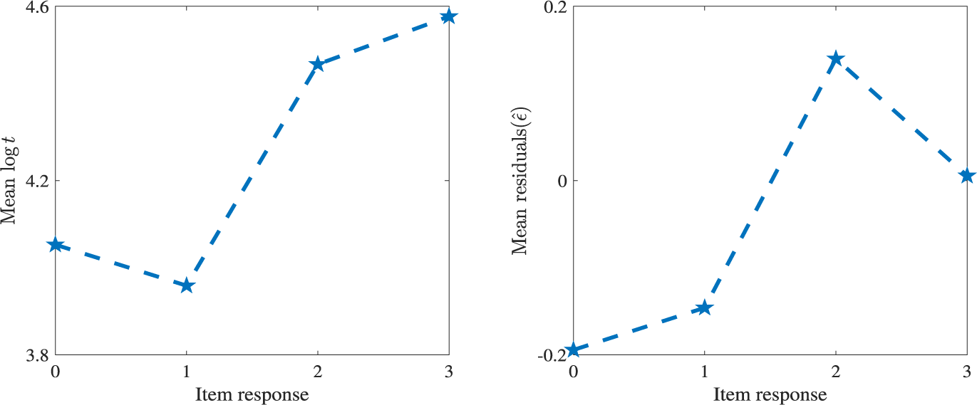


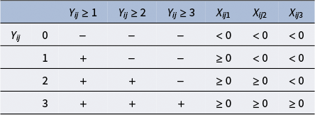


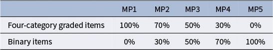


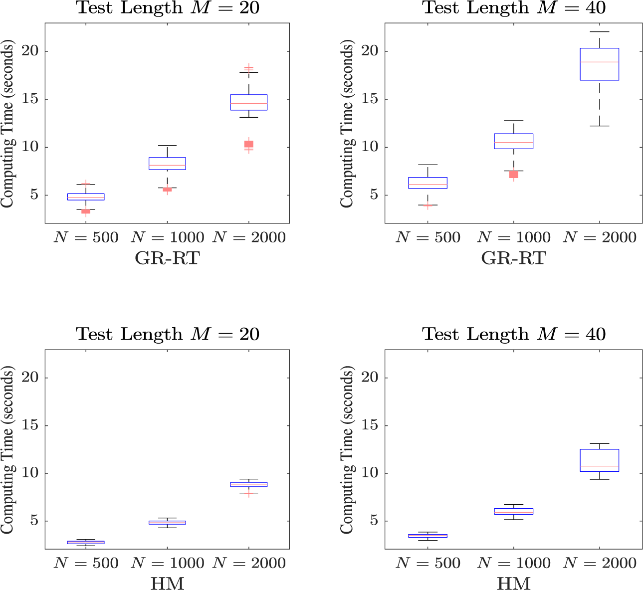


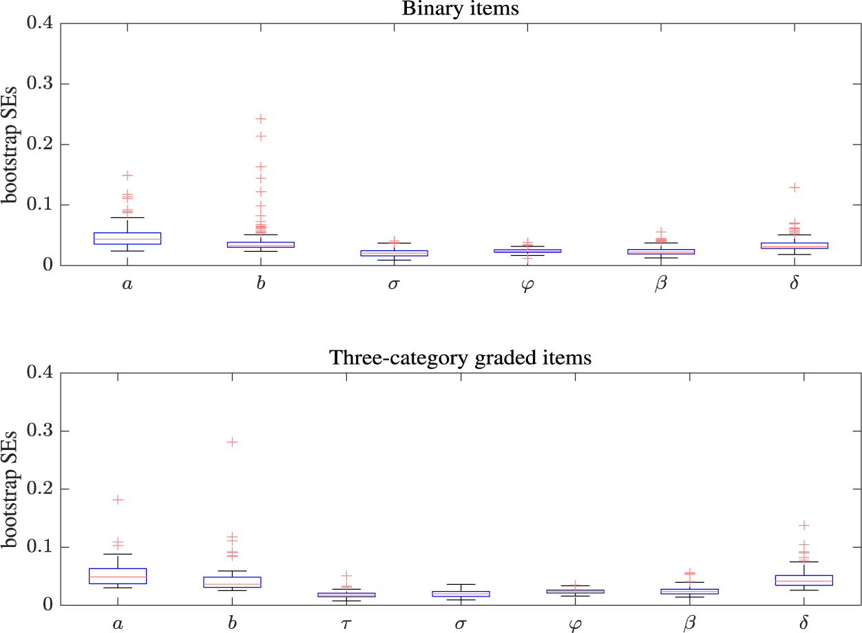
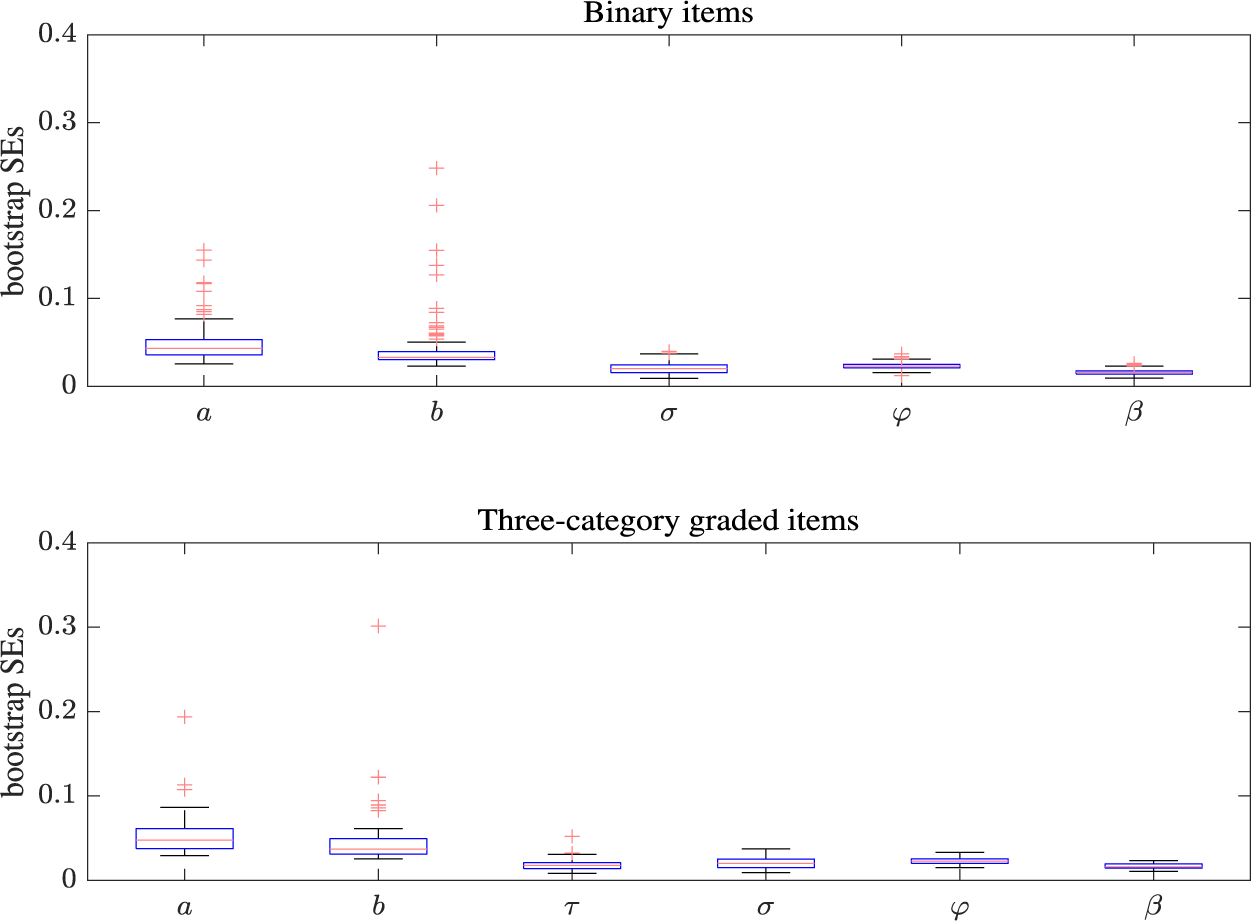
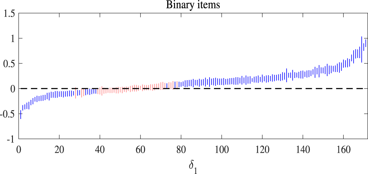

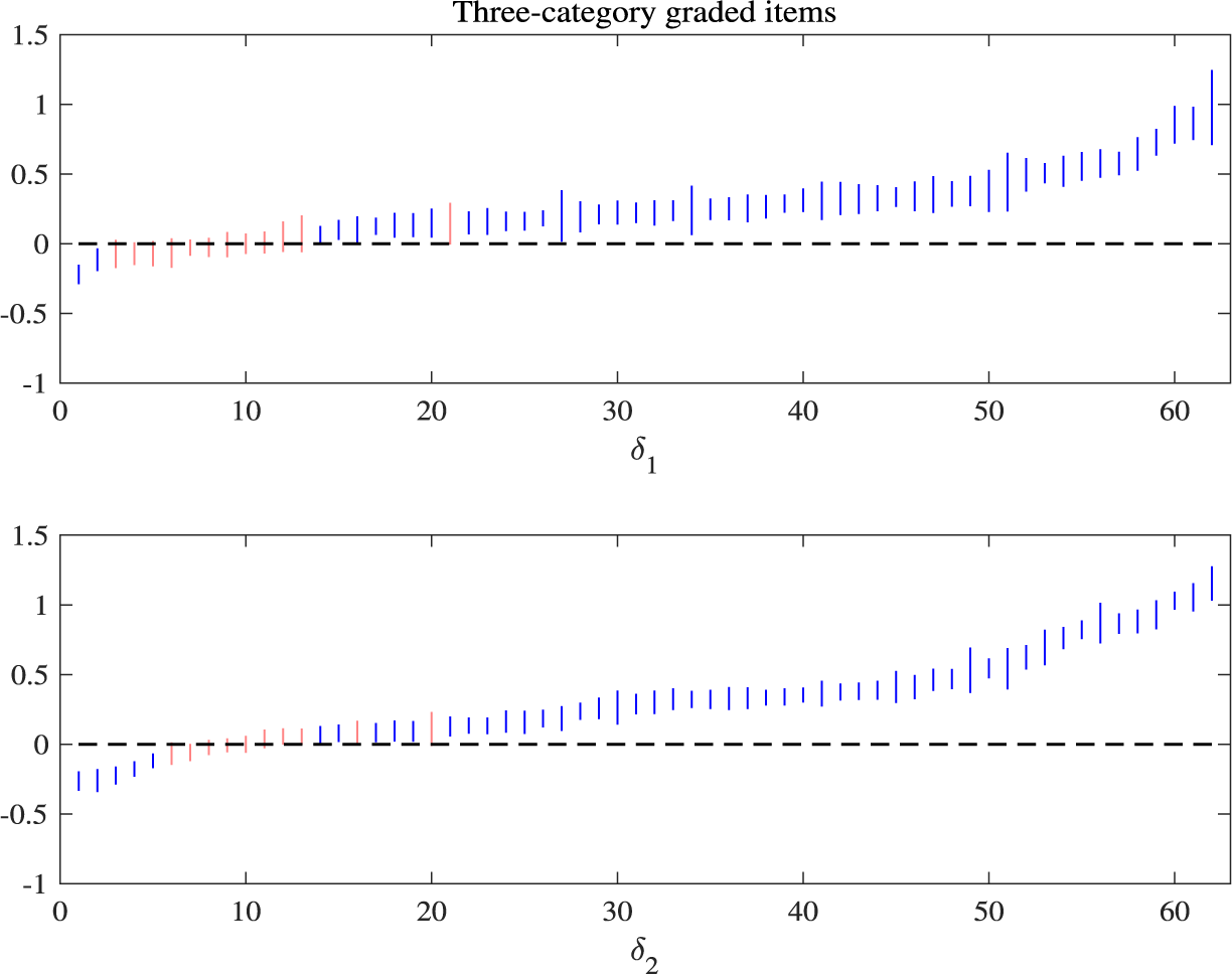


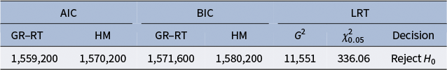


 Open access