


1. Introduction
The mechanical flow of ice is a product of the balance between the gravitational driving force that acts to move ice downstream and the resistive forces that counter this motion (Paterson, Reference Paterson1994). This counter force is influenced by the nature of the bed, such as thermal regime, material properties of the bed and roughness of the ice-bed interface. The quantitative description of subglacial topography is therefore important to understanding glacial dynamics (Hubbard and Hubbard, Reference Hubbard and Hubbard1998; Taylor and others, Reference Taylor, Siegert, Payne and Hubbard2004; Rippin and others, Reference Rippin, Bamber, Siegert, Vaughan and Corr2006), which is in meter scale roughness that relates to the basal sliding. Theories suggest that ice dynamics (particularly basal flow) are directly related to bed roughness at a range of spatial scales (Paterson, Reference Paterson1994; Joughin and others, Reference Joughin, Kwok and Fahnestock1998; Schoof, Reference Schoof2002), and this is increasingly regarded as an important research area in glaciology (Cooper and others, Reference Cooper2019). Li and others (Reference Li2010) showed that bed roughness derived from a frequency domain method applied to ice-penetrating radar data can be used to deduce the formation (marine or continental) and erosion history of a variety of end-case landscapes. Recently, bed roughness has also been used to simulate realistic digital elevation models and to locate subglacial lakes (e.g. Mackie and others, Reference Mackie, Schroeder, Caers, Siegfried and Scheidt2020; Goff and others, Reference Goff, Powell, Young and Blankenship2014). Clearly, a method that allows bed roughness to be extracted from radar data accurately and efficiently, with maximum information incorporated within the results, would allow it to become better assimilated into assessments of ice dynamics, glacial history and basal conditions (Eisen and others, Reference Eisen, Winter, Steinhage, Kleiner and Humbert2020).
The main methods of quantifying bed roughness from radar data can be divided into two categories: the electromagnetic scattering properties of the bed-echo waveform; and the statistical properties of the along-track topography (Cooper and others, Reference Cooper2019; Eisen and others, Reference Eisen, Winter, Steinhage, Kleiner and Humbert2020).
Analysis of electromagnetic scattering properties involves (1) waveform analysis (e.g. Cooper and others, Reference Cooper2019), (2) analysis of distribution of peak bed-echo power due to scattering loss (e.g. Grima and others, Reference Grima, Schroeder, Blankenship and Young2014), and (3) specularity analysis using different synthetic aperture sizes (e.g. Schroeder and others, Reference Schroeder, Blankenship and Young2013). Both theoretical predictions and observations demonstrate that specular reflections are suppressed in rougher regions (Jordan and others, Reference Jordan2017).
Methods that use statistical properties can be divided into those utilizing the ‘space domain’ and ‘frequency domain’. Space domain methods include some form of functional parameterization, such as the extraction of root-mean-square (rms) height, rms deviation, rms slope and autocorrelation length (Shepard and others, Reference Shepard2001; MacGregor and others, Reference MacGregor2013), from which variograms (rms height versus profile length) and deviograms (rms deviation versus horizontal lag) can be constructed, which have been well applied to glacier beds (MacGregor and others, Reference MacGregor2013; Jordan and others, Reference Jordan2017). In these methods, bed-roughness results vary with the lengths of the quantified profile or the spatial lag, often following a power-law trend with these lengths (Shepard and others, Reference Shepard2001). In the frequency domain, Hubbard and others (Reference Hubbard, Siegert and McCarroll2000) and Taylor and others (Reference Taylor, Siegert, Payne and Hubbard2004) defined a single-parameter roughness index as the integral of the spectrum within a specified interval, which can be used to extract the so-called ‘Hurst exponent’ (Martinez and others, Reference Martinez, Salgado, Cruz, Chavarin and Bustos2013) and the corner wavenumber. This single-parameter roughness index has two flaws, however: (1) it cannot be used directly to quantify slope bed irregularities, which leads to topography with different slope irregularities having similar roughness indices; and (2) it requires a fixed-size moving window (MW), which limits the scale of roughness quantified. Addressing the first issue, Li and others (Reference Li2010) designed a two-parameter roughness quantization method, which we call ‘the previous two-parameter method’ in this paper, that incorporates both vertical change and slope changes. However, this method is still problematic as it requires a fixed-size MW. The outcome is that large-scale roughness results do not incorporate small-scale terrain undulations, and vice versa. To solve this problem, the ‘wavelet transform’ method was developed. This technique uses different scales of MW, which means a variable-size MW, to divide the roughness signal at each position into components related to scale; the wavelet coefficients are the weight of each component (Boggess and Narcowich, Reference Boggess and Narcowich2015). Our method uses a range of scales like the wavelet transform method rather than a single-scale like the previous fast Fourier transform (FFT) methods.
Self-affine roughness (Jordan and others, Reference Jordan2017) is represented by the ‘Hurst exponent’ as a multi-scale roughness parameter that can accommodate a span of scales to a certain extent. In this method, problems occur in relation to ‘breakpoints’, however, where a power law appears to ‘break over’ and obey a different power law. This requires the investigator to subjectively choose where the beginning and endpoints of each trend occur when a breakpoint is evident (Shepard and others, Reference Shepard2001). Besides that, the ‘Hurst exponent’ results show rapid local fluctuations on maps (Jordan and others, Reference Jordan2017; Eisen and others, Reference Eisen, Winter, Steinhage, Kleiner and Humbert2020), which make it difficult to quantify the large span of terrains.
In this article, we describe a new algorithm to quantify bed roughness, improving the previous two-parameter method (Li and others, Reference Li2010) by accounting for different scales of roughness through a self-adaptive approach. In addition, the ‘scale’ we use in this paper is the horizontal length of the bed elevation profile which is quantified as roughness. In other words, the ‘scale’ in our method means the horizontal length of the FFT MW and the ‘scale’ in rms height method means the horizontal length of the quantified profile.
2 Methods
2.1 Outline and flowchart of the method
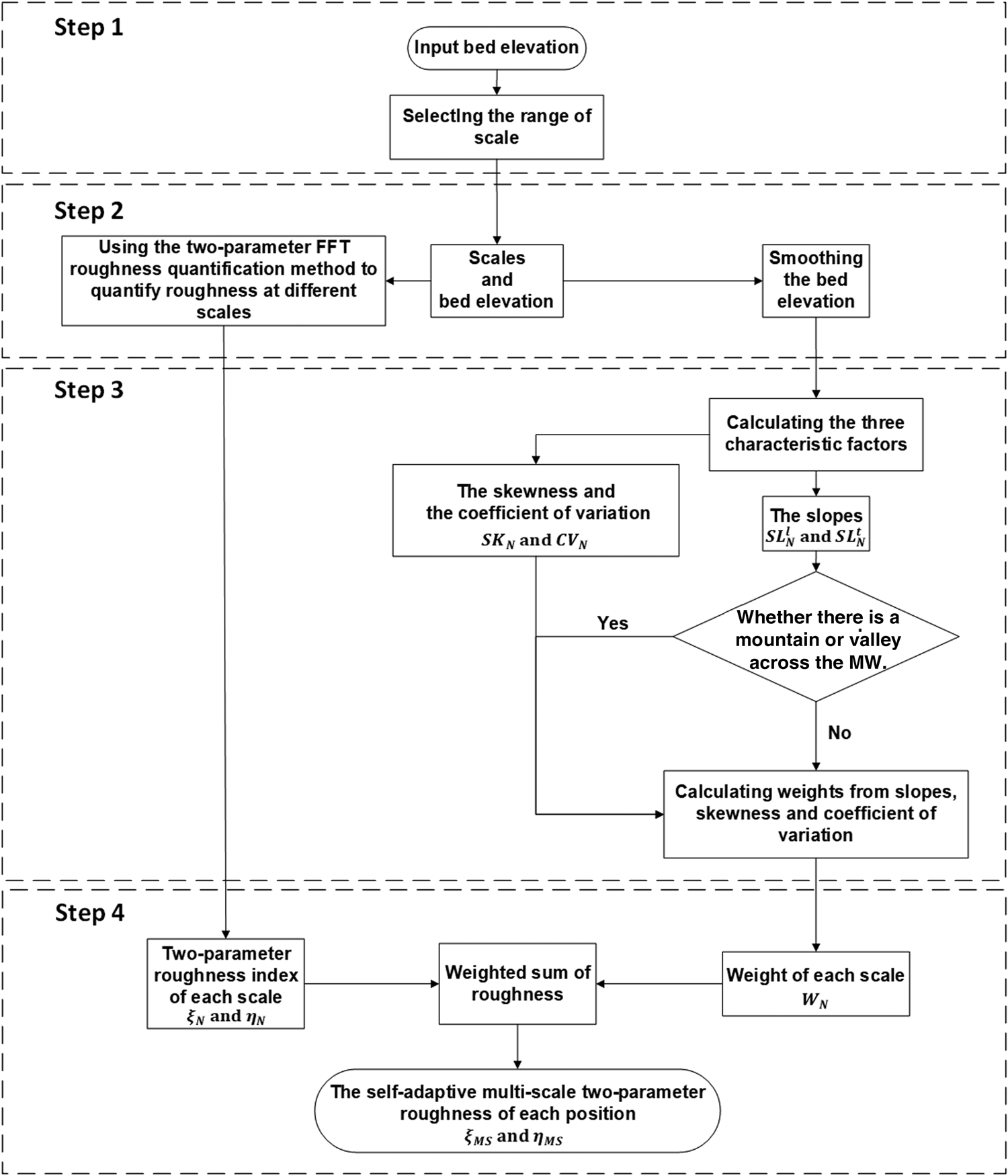
To solve the scale problem of the previous two-parameter method, we propose a self-adaptive two-parameter roughness quantization technique in four steps, as described in Figure 1.
Flowchart of the self-adaptive two-parameter roughness quantization method. The ‘scale’ we use in here refers to the horizontal length of the bed that is quantified as roughness. MW is moving window.
2.2 Step 1: selecting the range of scale
Our two-parameter roughness method, and the extraction of the characteristic factors, requires a bed elevation profile with a fixed sampling interval. It is therefore necessary to interpolate and resample bed data to ensure the method can work. The roughness, and the characteristic factors, of each position on the bed is calculated within the variable-size MW at multiple scales. The total number of along-track sample points in the MW is M = 2N, where N is the window-length exponent. Low-frequency fluctuations are observed on a large scale, and high-frequency fluctuations are observed in the small scale. We therefore calculate the roughness and the characteristic factors at multiple scales, which is analogous to the multi-scale decomposition of the wavelet transform. The scale range we need is equivalent to 102 − 104 m as it includes a variety of glacial bedforms that appear within this interval (e.g. drumlins, U-shaped valleys, crag and tails, etc.) (Ó Cofaigh and others, Reference Ó Cofaigh, Pudsey, Dowdeswell and Morris2002; Stokes and Clark, Reference Stokes and Clark2003).
2.3 Step 2: calculating the two-parameter roughness of different scales
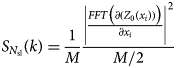
The first parameter ξN(x i) of the two-parameter roughness index, whose unit is m2 (Li and others, Reference Li2010), describes the magnitude of vertical deviations in the bed slope, and is calculated by:
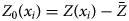
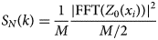
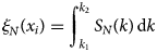
where x corresponds to the location in the bedrock; x i is the position of the point in the variable-size MW (1 ≤ i ≤ M); Z(x i) denotes the bed elevation; $\bar Z$ is the mean of Z(x i) in the variable-size MW; Z 0(x i) is the mean-detrended profile; S N(k) is the spectral power density of Z 0(x i); k is the angular frequency; and k 1 is zero and k 2 is infinity.
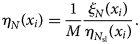
The second parameter η N(x i), whose unit is m2 (Li and others, Reference Li2010), quantifies the slope frequency of these deviations, and is obtained using the ratio of the first parameter defined in equation (1) to the slope index. The slope index is calculated using the FFT to convert the slope of the bed elevation profile into the average power. We obtain the slope index $\eta _{N_{{\rm sl}}}\lpar x_i\rpar$ , by:
, by:
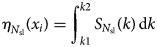
where $S_{N_{{\rm sl}}}\lpar k\rpar$ is the spectral power density of the slope profile ${\partial \lpar Z_0\lpar x_i\rpar \rpar \over \partial x_i}$
 . Finally, we obtain η N(x i) as follows,
2.4 Step 3: calculating the weights
Three characteristic factors are used to estimate the shape of the bed elevation profile: (1) the slopes, (2) the skewness and (3) the coefficient of variation. They are calculated simultaneously with the variable-size MW.
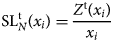
The slopes are usually used to indicate how inclined a curve is, which include the leading and trailing edge steepness. The leading-edge steepness ${\rm SL}_N^{\rm l}\lpar x_i\rpar$ of the bed elevation Z(x i) within the variable-size MW is estimated by:
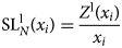
where Z l(x i) is the leading edge of the bed elevation. Similarly, the trailing edge steepness, denoted as ${\rm SL}_N^{\rm t}\lpar x_i\rpar$ , is calculated by:
where Z t(x i) is the trailing edge. The visualized examples of ${\rm SL}_N^{\rm l}\lpar x_i\rpar$ and ${\rm SL}_N^{\rm t}\lpar x_i\rpar$
 are shown in Figure 2. The ${\rm SL}_N^{\rm l}\lpar x_i\rpar$
 and ${\rm SL}_N^{\rm t}\lpar x_i\rpar$
 quantify the leading and trailing edge steepness, respectively.
The leading and trailing edge steepness ${\rm SL}_N^{\rm l}\lpar x_i\rpar$ and ${\rm SL}_N^{\rm t}\lpar x_i\rpar$
 , the skewness SKN(x i) and the coefficient of variation CVN(x i) for N = 10 of four parts of bed elevation profile of TT’ in Figure 4. The red line represents ${\rm SL}_N^{\rm l}\lpar x_i\rpar$
 and the green line represents ${\rm SL}_N^{\rm t}\lpar x_i\rpar$
 . (a) From 136 to 156 km of TT’. (b) From 278 to 298 km of TT’. (c) From 26 to 46 km of TT’. (d) From 145 to 165 km of TT’.
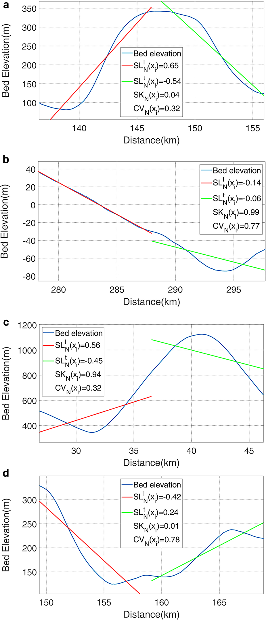
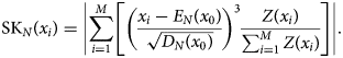
In general, skewness, which quantifies the degree of asymmetry of a curve (i.e. the larger the value, the greater the asymmetry) (Moore and Kirkland, Reference Moore and Kirkland2007), is a measure of the direction and degree of deviation of the bed elevation profile from its center. Firstly, we calculate the expectation value, E N(x i), and the variance, D N(x i), of the bed elevation profile as follows:
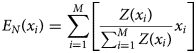
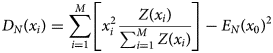
where x 0 denotes the center of the variable-size MW. Next, we calculate the skewness by:
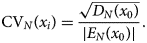
The coefficient of variation is a measure of the relative dispersion (Yadolah, Reference Yadolah2008), and is calculated by:
The visualized examples of SKN(x i) and CVN(x i) are shown in Figure 2. As we can see in Figure 2, we chose a mountain, two slopes and a valley as examples. The mountain is symmetrical, leading to low values of both SKN(x i) and CVN(x i). The slopes are asymmetrical and so SKN(x i) and CVN(x i) will both be high or high SKN(x i) and low CVN(x i). The valley can lead to low SKN(x i) and high CVN(x i).
By evaluating the value of ${\rm SL}_N^{\rm l}\lpar x_i\rpar$ , ${\rm SL}_N^{\rm t}\lpar x_i\rpar$
 , SKN(x i) and CVN(x i) from Eqn (7–12), we can quantify the shape of terrain (Khan and others, Reference Khan, Aleem and Shah2011; Ilisei and others, Reference Ilisei, Khodadadzadeh, Ferro and Bruzzone2018), from which we obtain the weight, W N(x i), of each scale. More detail about how to obtain the weights and how the weights change with the three characteristic factors can be found in Appendix A and Appendix B, respectively.
2.5 Step 4: calculating the self-adaptive two-parameter roughness index
Finally, the self-adaptive first and second parameter roughness index, ξMS(x i) and η MS(x i), are calculated by weighting and summing the roughness of the different scales in Eqn (1) and (3):
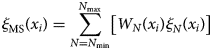
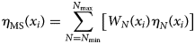
where N min and N max are the range of N. ξMS(x i) and η MS(x i) are then the self-adaptive two-parameter roughness index.
3. Experiments
3.1 Simulated bed elevations
Since the sampling interval of bed elevations that we use later is ~19 m (Cui and others, Reference Cui2018), and the variable-size MW should be in the range of 102 − 104 m as mentioned above, we use 5 ≤ N ≤ 10 and M = 25 − 210(608 − 19456 m) to process the real bed elevation dataset. Hence, the simulated bed elevation that we used here has 1024 sample points.
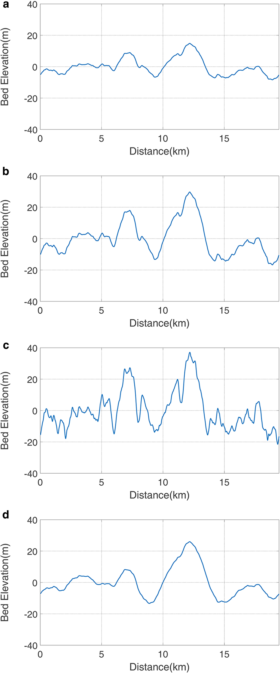
To prove the effectiveness of the algorithm in quantifying roughness, we compare the quantization results of the simulated beds’ roughness with a variety of irregularities, described in Figure 3. The simulated bed profiles are generated using a self-correlation function (Thomas, Reference Thomas1999; Li and others, Reference Li2010). Two controllable inputs, which are standard deviation and autocorrelation length, are used to control the vertical and slope irregularities of the bed, respectively. As we increase the standard deviation but keep the autocorrelation length unchanged, the bed elevation profile transforms from that in Figures 3a to b. Accordingly, our self-adaptive first parameter roughness index ξMS(x i) increases and our self-adaptive second parameter roughness index η MS(x i) is unchanged. On the other hand, if the standard deviation is unchanged but autocorrelation length is increased, the bed elevation profile changes from that in Figures 3b to c. In this case, ξMS(x i) is unchanged and η MS(x i) reduces. Similarly, when the standard deviation is unchanged and autocorrelation length is reduced, which means the bed changes from that in Figures 3b to d, ξMS(x i) is unchanged and η MS(x i) increases. Theoretically, higher values of the first roughness parameter relate to higher vertical roughnesses; whereas lower values of the second parameter roughness correspond with higher slope roughnesses (Li and others, Reference Li2010). This simple analysis shows that the method is working as it should, and can now be applied to more complex, real-world examples. The comparison between the results of our self-adaptive two-parameter method, the previous two-parameter method and the Hurst exponent method in a simulated bed elevation profile can be found in Appendix C.
Random simulated bed elevation profiles with four different roughness. (a) Our self-adaptive first and second parameter roughness index, whose unit is m2, ξMS(x i) = 0.34, η MS(x i) = 1906.1. (b) ξMS(x i) = 1.35, η MS(x i) = 1906.1. (c) ξMS(x i) = 1.35, η MS(x i) = 455.0. (d) ξMS(x i) = 1.35, η MS(x i) = 7347.3.
3.2 Real bed elevations
The radar profile used in this study was acquired in CHINARE 33 by the Snow Eagle 601, which is a modified DC-3 aircraft fully equipped with a suite of geophysical instruments. The apparatus of relevance to this paper is the airborne ice sounding radar, functionally similar with the High Capability Airborne Radar System (HiCARS), which uses a double flat-plate dipole antenna with a peak power of 8 kW and a center frequency of 60 MHz. The radar can penetrate Antarctic ice to a depth of more than 3 km, and can measure internal reflection horizons with a high detection resolution (Cui and others, Reference Cui2018).
The radar data were processed using along-track coherent stacking, pulse compression and along-track incoherent stacking. The data resolution in the along-track direction is ~19 m after the process of interpolation and resampling, and the depth resolution is ~10 m in air and ~5.6 m in ice (Cui and others, Reference Cui2018). The bed-ice interfaces were traced and digitized by a semi-automatic program, using the manually picked lower and upper boundaries of the bed interface as a constraint on automatic bed interface picking (Cui and others, Reference Cui2020). The program was also used to process the former ICECAP data from the Aurora and Wilkes subglacial basins (Blankenship and others, Reference Blankenship2016, Reference Blankenship2017).
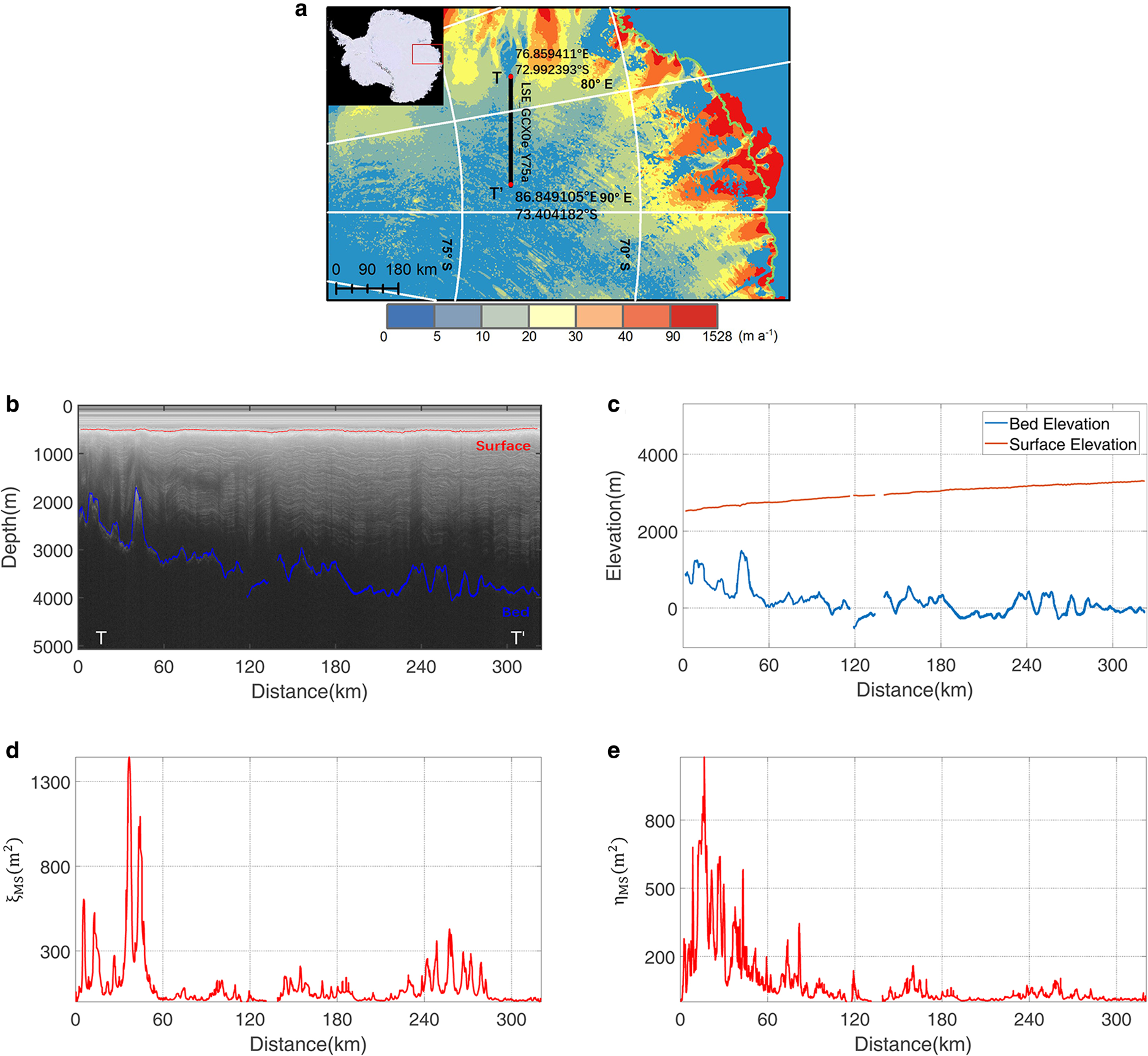
In this paper, we have analyzed the radar profile ‘LSE_GCX0e_Y75a’, which is referred to as TT’ and has a length of 323.9 km. The radar profile is shown in Figure 4b, and its bed elevation and ice-surface are shown in Figure 4c. The roughness results from our algorithm are shown in Figures 4d and e. The radar profile is located between ~ 77°E and ~ 87°E in an approximate west-east direction, covering a region with low ice-flow speed, ranging from 0 to 20 m~a−1 (Fig. 4a). The bed elevations are high between 0 and 60 km, and elsewhere vary closer to the sea level with a relatively low amplitude of several hundred meters. An obvious mountain occurs between ~35 and 55 km, and two relatively smooth areas appear between ~190 and ~230 km and between ~280 km and the end of the profile.
The profiles of LSE_GCX0e_Y75a (TT’). (a) Ice velocity map and location of TT’. Ice velocity map is from the MEaSUREs InSAR-Based Antarctica Ice Velocity Map, Version 2 (Rignot and others, Reference Rignot, Mouginot and Scheuchl2017). Grounding lines are shown in green. (b) Ice-sounding radar profile. (c) Ice-surface elevation and bed elevation. Our self-adaptive first and second parameter roughness index (d) ξMS(x i) and (e) η MS(x i).
3.3 Comparison of results
3.3.1 The Hurst exponent
The statistical methods used to calculate the Hurst exponent (H), and thus to quantify the self-affine scaling behavior, are well established in the literature (Malinverno, Reference Malinverno1990; Shepard and others, Reference Shepard2001; Kulatilake and others, Reference Kulatilake, Um and Pan1998; Orosei and others, Reference Orosei2003). A feature of terrain with a higher H is that it tends to appear relatively rough at larger length scales (low frequencies) and smooth at smaller length scales (high frequencies). A feature of lower H terrain is that it tends to have similar roughness across different length scales (Jordan and others, Reference Jordan2017). We used the rms height, R(L), to extract the Hurst exponent:
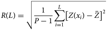
where P is the number of sample points within the profile window; and L is the length of the profile window. We then extract the Hurst exponent H by the rms height as follows:
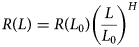
where L 0 is a reference profile length. As L increases, R(L) also increases, as they have a linear relationship. Thus, the Hurst exponent H is the slope of L and R(L). The Hurst exponent is a multi-scale standardized result that can be compared with the rms height, or slopes of different surfaces, as measured by different tools at similar scales (Shepard and others, Reference Shepard2001).
3.3.2 Roughness comparisons
Profile TT’ crosses the Kronshtadtskiy Glacier. The first 50 km is characterized by high ξMS(x i) and high η MS(x i), while the other sections are mainly characterized by low ξMS(x i) and low η MS(x i) roughness (Figs 4d and e). We now focus on the mountain at about 40 km (Fig. 5). Comparing the roughness results of the profile at this place, we can see that ξMS(x i) and ξN(x i) each have peaks. But ξN(x i) shows very low values from 39 to 42 km, and ξMS(x i) shows high values representing the span of the mountain. η MS(x i) has several very low peaks, indicative of high roughness, in contrast to η N(x i). The trend of Hurst exponent, η MS(x i) and η N(x i) is roughly the same, as described in Figure 5c.
A part of roughness of profile TT’ (from 32 to 52 km). The marked points locate in the center of the profile. (a) The bed elevation profile. (b) Our self-adaptive first parameter roughness index ξMS(x i) and Li's first parameter roughness index ξN(x i). (c) Our self-adaptive second parameter roughness index η MS(x i), Li's second parameter roughness index η N(x i) and the Hurst exponent H. The ξN(x i) and ηN(x i) are calculated when N = 5.
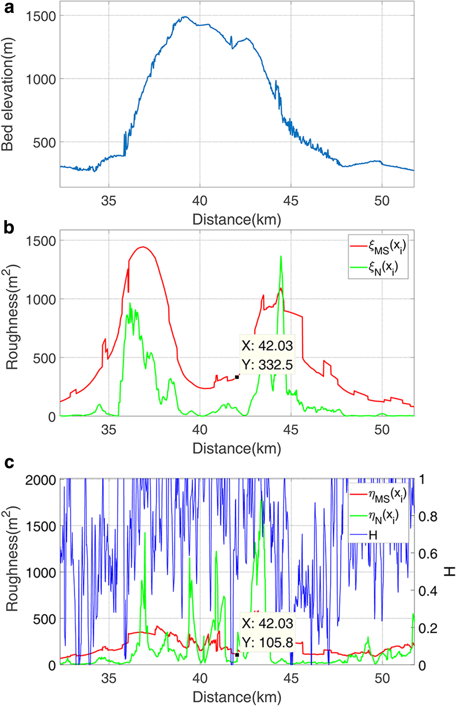
Li et al. (Reference Li2010)'s first and second parameter roughness index ξN(x i) and η N(x i) are sensitive to the MW size. To prove this, we calculate ξN(x i) = 55.1 and η N(x i) = 32.9 at N = 5 in the central position of the profile, as shown in Figure 5. We then calculate ξN(x i) and η N(x i) in same position while increasing N, revealing differences in both ξN(x i) and η N(x i) (i.e. ξN(x i) = 30.1 and η N(x i) = 22.9 at N = 6; ξN(x i) = 66.0 and η N(x i) = 86.3 at N = 7; ξN(x i) = 431.9 and η N(x i) = 123.4 at N = 8; ξN(x i) = 800.4 and η N(x i) = 195.2 at N = 9; and ξN(x i) = 611.4 and η N(x i) = 174.0 at N = 10). In contrast, our self-adaptive first and second parameter roughness index ξMS(x i) = 332.5 and η MS(x i) = 105.8 are stable across the scale range, as shown in Figures 5b and c. The unit of ξN(x i), η N(x i), ξMS(x i) and η MS(x i) is m2 (Li and others, Reference Li2010).
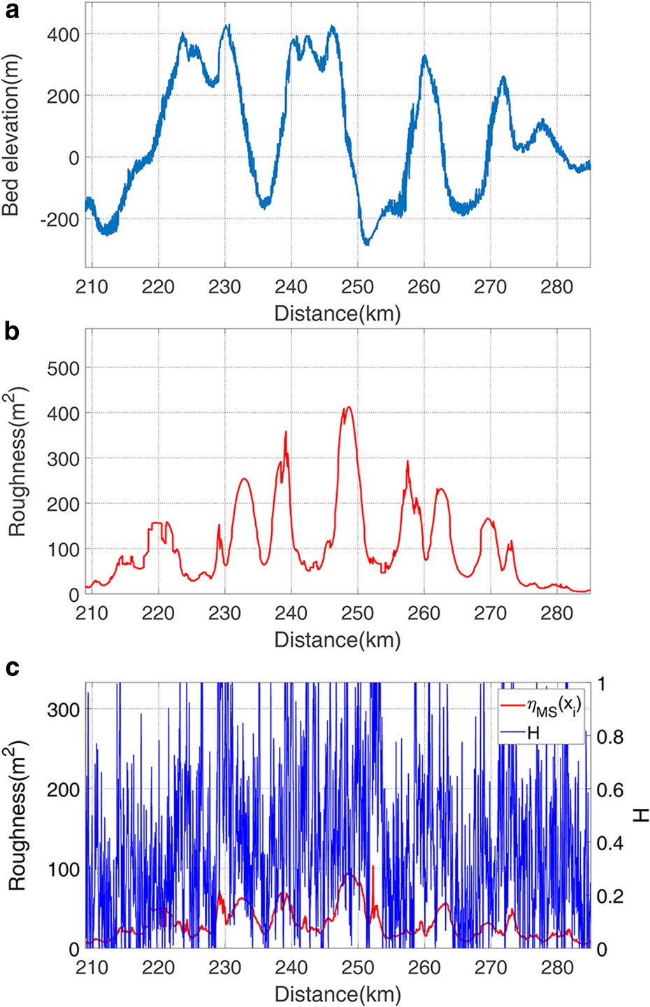
Through the last 76 km of TT’, we can see several mountain peaks and valleys (Fig. 6). By comparing the η MS(x i) and H of the profile in this place, we can see that η MS(x i) has several very low peaks, indicative of high roughness, but the Hurst exponent has too many peaks to resolve (Fig. 6c).
A part of roughness of profile TT’ (from 209 to 285 km). (a) The bed elevation profile. (b) The roughness index ξMS(x i). (c) The roughness index η MS(x i) and the Hurst exponent H.
4. Conclusions
We describe a new method to determine subglacial topographic roughness, called the ‘self-adaptive two-parameter roughness quantization’ method. The algorithm is based on the two-parameter roughness quantization method and is analogous to a wavelet transform. According to the weights calculated from three characteristic factors, the new algorithm can determine the scale needed to quantify the roughness at any position. This eliminates the problem of a fixed-size MW of measurements being unable to cope with roughness at multiple scales.
We use simulated bed elevations to test the new algorithm, demonstrating hypothetically the effectiveness of the new algorithm in quantifying roughness. In cases where real bed elevations are used, we show that the algorithm can achieve a better characterization of roughness than the previous two-parameter method. Comparisons between the results of our self-adaptive two-parameter method, the previous two-parameter method and the Hurst exponent method show the advantage of our approach in capturing different scales of terrain span and demonstrate the effectiveness of the new algorithm in quantifying bed roughness.
This method provides an improved tool for quantifying the roughness of the subglacial environment from a multi-scale perspective, especially in the analysis of complex subglacial topography. The new method offers a means by which multi-scale roughness can be quantified at a continental scale. Such a product would have significant glaciological applications, especially in distinguishing between erosional and depositional landscapes. The method could be applied to higher along-track resolution data if it is available in the future for evaluating the magnitude and distribution of basal sliding at the meter scale. The method works particularly well over subglacial landscapes with horizontal lengths greater than the length of a traditional fixed-size MW (e.g. mountains and valleys), resolving the roughness in all places. It also works well in landscapes that have notable roughness at a scale less than a fixed-size MW, as it is able to incorporate the fine-scale roughness within the wider terrain.
The code/routines of the self-adaptive two-parameter roughness quantization method will be freely available under requests from any researchers. We hope the new method can be extensively used by the community to characterize subglacial roughness in future.
Acknowledgements
This work was supported by the National Natural Science Foundation of China (Nos. 41941006, 41606219, 41776186), the National Key R&D Program of China (2019YFC1509102), the Scientific Research Project of Beijing Educational Committee (No. KM201910005027) and the Rixin Foundation of Beijin University of Technology. M.J.S. was supported by a British Council ‘Global Innovation Initiative’ award. We also thank the anonymous reviewers for their positive comments and suggestions for improving this paper and editors for editing this paper.
Appendix A. Calculating the weight
By evaluating the value of ${\rm SL}_N^{\rm l}\lpar x_i\rpar$ , ${\rm SL}_N^{\rm t}\lpar x_i\rpar$
 , SKN(x i) and CVN(x i) from Eqn (9–12), we can quantify the shape of terrain, from which we obtain the weight, W N(x i), of each scale as follows,
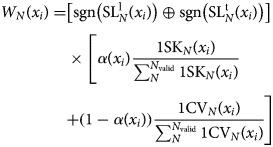
where N valid are the scales at $[ {\rm sgn}\lpar {\rm SL}_{N_{{\rm valid}}}^{l}\lpar x_i\rpar \rpar \oplus {\rm sgn}\lpar {\rm SL}_{N_{{\rm valid}}}^{t}\lpar x_i\rpar \rpar \rsqb = 1$ ; sgn( · ) is the sign function that if · >0 return 1 and if · <0 return -1; $\oplus$
 is the exclusive or (xor) function. The α(x i) is the parameter for adjusting the influence of SKN(x i) and CVN(x i) on the weight distribution, which is calculated by:
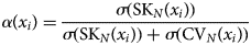
where $\sigma \lpar {\rm SK}_N\lpar x_i\rpar \rpar = \sqrt {{\sum _{N}^{N_{{\rm valid}}} [ {\rm SK}_N\lpar x_i\rpar - \overline { {\rm SK}}_{N_{{\rm valid}}}\lpar x_i\rpar \rsqb ^{2}\over {\rm count}\lpar N_{{\rm valid}}\rpar }}$ is the standard deviation of SKN(x i), which is same for σ(CVN(x i)); count(N valid) is the count of the N valid; $\overline {{\rm SK}}_{N_{{\rm valid}}}\lpar x_i\rpar$
 is the mean of SKN(x i) at N = N valid. The greater the measure of dispersion of SKN(x i), the greater the α(x i), which is same for CVN(x i) and 1 − α(x i).
Appendix B. Three characteristic factors and the associated weights
The changes in the weight W N(x i) with the skewness SKN(x i) and the coefficient of variation CVN(x i) at N = 10 are shown in Figure 7. To make it easier to understand, we discard the SKN(x i) and CVN(x i) at $[ {\rm sgn}\lpar {\rm SL}_N^{\rm l}\lpar x_i\rpar \rpar \oplus {\rm sgn}\lpar {\rm SL}_N^{\rm t}\lpar x_i\rpar \rpar \rsqb = 0$ .
.
The changes in the weight W N(x i) with the skewness SKN(x i) and the coefficient of variation CVN(x i) at N = 10. The example is located in a part of profile TT’ (from 22 to 62 km).
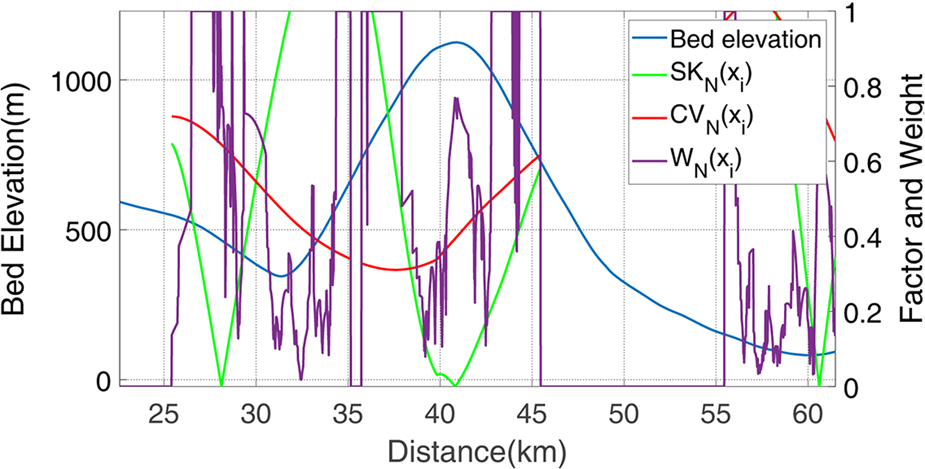
When other conditions remain unchanged, both low values of SKN(x i) and CVN(x i) will make the W N(x i) high like the part from 41 to 42 km. The W N(x i) at N = 10 is also influenced by SKN(x i), CVN(x i) and $[ {\rm sgn}\lpar {\rm SL}_N^{\rm l}\lpar x_i\rpar \rpar \oplus {\rm sgn}\lpar {\rm SL}_N^{\rm t}\lpar x_i\rpar \rpar \rsqb$ at N ≠ 10 like the part from 36 to 37 km that $[ {\rm sgn}\lpar {\rm SL}_N^{\rm l}\lpar x_i\rpar \rpar \oplus {\rm sgn}\lpar {\rm SL}_N^{\rm t}\lpar x_i\rpar \rpar \rsqb = 0$
 at N = 5–9.
Appendix C. Comparison of roughness results in a simulated bed elevation profile
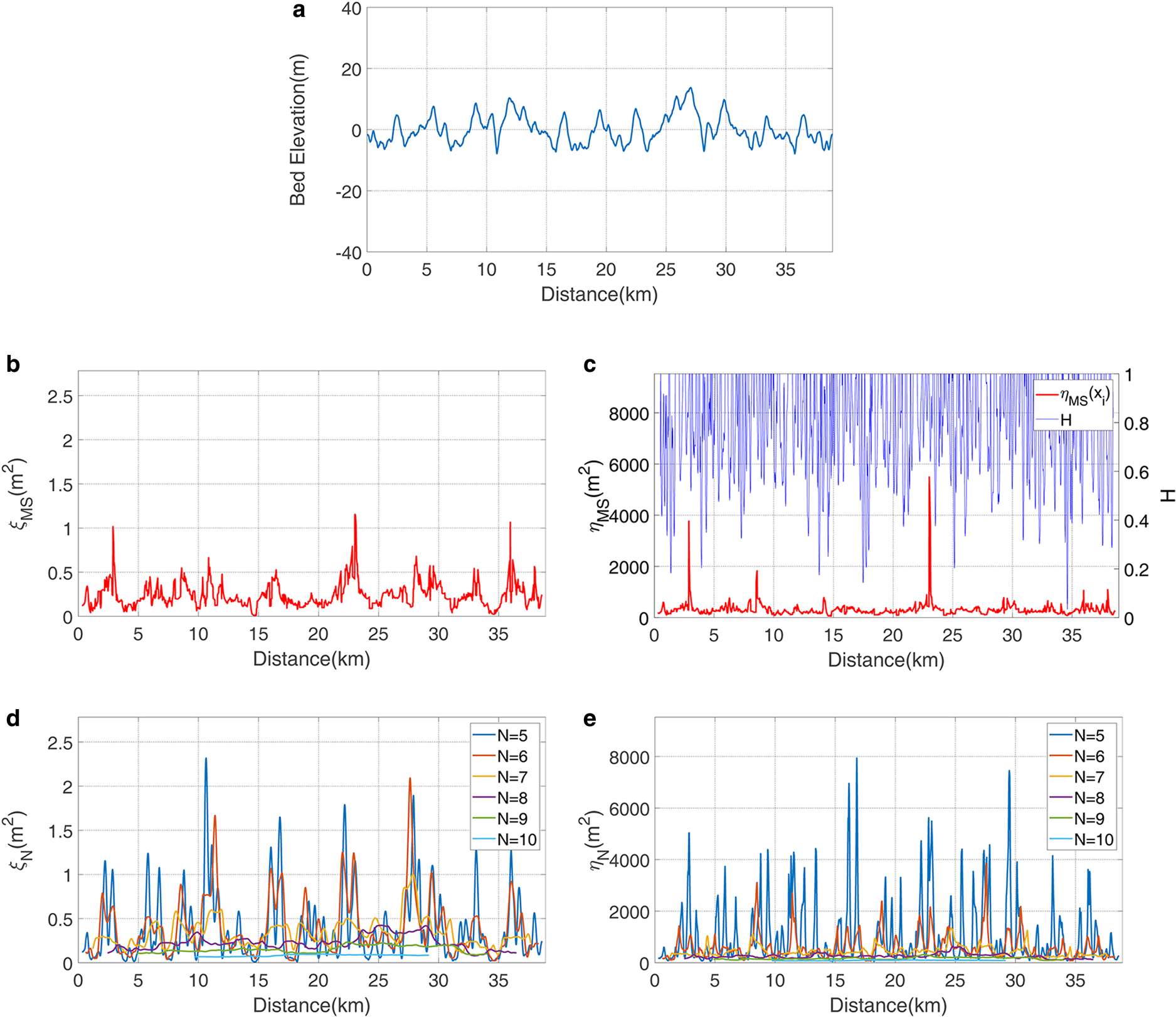
We compare the results of our self-adaptive two-parameter method with the results of the previous two-parameter method and the Hurst exponent method in a simulated bed elevation profile shown in Figure 8, which demonstrate the Li's first and second parameter roughness index ξN(x i) and η N(x i) are sensitive to the scale and the Hurst exponent H has the shortcoming of rapid fluctuations. In contrast, our self-adaptive first and second parameter roughness index ξMS(x i) and η MS(x i) are stable across the scale range.
The roughnesses of simulated bed elevation profile. (a) Random simulated bed elevation profile about 40 km long; our self-adaptive first and second parameter roughness index (b) ξMS(x i), (c) η MS(x i) and Hurst exponent H; Li's first and second parameter roughness index (d) ξN(x i), and (e) η N(x i).


 Open access