


1. Introduction
Across the high-altitude dry snow zone areas of the vast Greenland and Antarctic Ice Sheets where the snow rarely melts, surface snow compacts over time as new snow falls on top each year. As it compacts over years, it undergoes post-depositional metamorphism to become ‘firn’, which is porous ice many tens of meters deep between the recent surface snow and underlying solid glacial ice. Innovations in satellite technology have enabled increasingly precise remote sensing of the ice sheets, using electromagnetic signals to detect characteristics meters deep in near-surface firn (e.g., Winsvold and others, Reference Winsvold2018; Barzycka and others, Reference Barzycka2020). The remote-sensing capability in turn has sparked innovations in ice-sheet modeling. To accurately interpret the satellite data, and for use in ice-sheet and regional climate modeling, knowledge of the effective thermal conductivity of firn is needed, yet published direct measurements of the effective thermal conductivity of polar firn as a function of depth below several meters do not exist. This research presents direct measurements of the thermal conductivity of polar firn over many tens of meters.
The metamorphism of firn changes its structure and material properties beyond its original state as seasonal snow. Although snow and firn have different physical characteristics, techniques for measuring the thermal conductivity of snow may also be appropriate for firn. Several techniques will be briefly described here. The needle probe method is a transient measurement technique which employs a thin needle that is inserted into a material and briefly heated; the resulting temperature rise in the material is measured and used to infer the thermal conductivity. This technique is appreciated for its rapid results and has been implemented by many snow and firn researchers, starting with Jaafar and Picot (Reference Jaafar and Picot1970) over a half-century ago. Needle probes have been frequently used to measure the thermal conductivity of snow (e.g., Sturm and Johnson, Reference Sturm and Johnson1992; Singh, Reference Singh1999; Sturm and others, Reference Sturm, Perovich and Holmgren2002; Aggarwal and others, Reference Aggarwal, Negi and Satyawali2009; Morin and others, Reference Morin, Domine, Arnaud and Picard2010; Calonne and others, Reference Calonne2011). Sturm and others (Reference Sturm, Holmgren, König and Morris1997) provide a review of many earlier implementations of this method in snow. Needle probes have also been used on firn, though the scope of the measurements is limited: Lange (Reference Lange1985) and Courville and others (Reference Courville, Albert, Fahnestock, Cathles and Shuman2007) collected measurements using needle probes on snow and polar firn to depths of 2.5 and 4 m, respectively. Recently, the accuracy of needle probe measurements in snow and firn has come into question, as the needle can cause damage to the local microstructure (Riche and Schneebeli, Reference Riche and Schneebeli2010), and the method has been found to provide underestimations of the thermal conductivity by a factor of 2 to 3 (Riche and Schneebeli, Reference Riche and Schneebeli2013).
A second technique is the guarded hot plate method, whereby one end of a sample is heated and measurements are made of the heat flux through that sample and the temperatures at either end of the sample, all of which are then used to calculate its one-directional effective thermal conductivity. This laboratory process takes longer to complete compared to the needle probe method, though it provides more accurate results (Riche and Schneebeli, Reference Riche and Schneebeli2013). The guarded hot plate has been successfully implemented in snow research (e.g., Pitman and Zuckerman, Reference Pitman and Zuckerman1967; Schneebeli and Sokratov, Reference Schneebeli and Sokratov2004). To the present authors’ knowledge, the thermal conductivity of firn has never been measured using the guarded hot plate method.
Numerical simulations offer another method for estimating the thermal conductivity of materials such as snow or firn. This method requires properly defining the sample's microstructure, for example, by micro-CT imaging, with use of the resulting information in a numerical model to predict the rate of heat conduction through the sample (e.g., Kaempfer and others, Reference Kaempfer, Schneebeli and Sokratov2005; Calonne and others, Reference Calonne2011, Reference Calonne2019). This process can be time consuming. Similar to the guarded hot plate, this method has also been shown to provide accurate thermal conductivity measurements (Riche and Schneebeli, Reference Riche and Schneebeli2013).
The method of inverting in-situ temperature measurements is an indirect method to estimate the bulk effective thermal conductivity. Using inverse simulation techniques, Marchenko and others (Reference Marchenko2019) estimated the effective thermal conductivity of firn using in-situ temperature measurements in the top 10 m of firn at Lomonosovfanna, Svalbard. Similarly, Giese and Hawley (Reference Giese and Hawley2015) and Clemens-Sewall and others (pers. comm. 2021) provide estimations of the effective thermal diffusivity of firn using in-situ temperature measurements in the top 30 m of firn at Summit Station, Greenland, and in the top 10.5 m of firn at various sites, respectively. This technique has also been applied to surface snow, where the sample depth was much smaller than these firn depths (Oldroyd and others, Reference Oldroyd, Higgins, Huwald, Selker and Parlange2013).
Firn has different microstructural characteristics than seasonal snow due to its significant post-depositional metamorphism and sintering processes that occur over long times, from years to many decades; measurements of the thermal conductivity of snow are not suitable for firn (Calonne and others, Reference Calonne2019). In this paper, we present direct measurements of the effective thermal conductivity of firn down to depths of 48 m using the guarded hot plate method. In the following sections, the custom guarded hot plate development and verification is described, followed by a description of the device's use to measure the thermal conductivity of firn core samples that were retrieved from the East Antarctic Ice Sheet at the South Pole. The associated thermal diffusivities of the firn samples are also presented. These thermal conductivity and thermal diffusivity measurements are then compared to existing estimation techniques and measurements, and equations for estimating the thermal conductivity of firn based on our measurements are presented.
2. Background
2.1. Estimations based on firn and snow
The limited number of direct measurements of the thermal conductivity of firn has caused a lack of formulas for estimating the thermal conductivity of firn. Instead, modelers have used or extrapolated formulas that had originally been designed to estimate the thermal conductivity of snow; formulas for snow are not suitable to firn due to the significant differences in microstructure between seasonal snow and polar firn. Calonne and others (Reference Calonne2019) succinctly summarized the existing equations available for predicting the thermal conductivity of snow and firn and further provide information on the temperature ranges in which they are applicable. Subsequently, they used a 3D images-based computation technique to derive a formula applicable for estimating the thermal conductivity intended for all densities and temperatures of snow, firn and porous ice. The equations of Van Dusen (Reference Van Dusen1929) and Schwerdtfeger (Reference Schwerdtfeger1963) have been used to estimate the lower and upper bounds of the effective thermal conductivity of snow, respectively (Cuffey and Paterson, Reference Cuffey and Paterson2010). These equations are shown in Table 1.
Existing equations commonly used to estimate the thermal conductivity of firn

For the equation of Calonne and others (Reference Calonne2019), the accompanying formulas and methodology for determining θ, $k_{{\rm firn}}^{{\rm ref}}( \rho )$ and $k_{{\rm snow}}^{{\rm ref}}( \rho )$
 should be viewed in the original publication.
3. Methods
3.1. Firn samples and site location
This research focuses on firn from the top 48 m of the East Antarctic Ice Sheet at the South Pole. The mean air temperature at South Pole is − 49°C (Lazzara and others, Reference Lazzara, Keller, Markle and Gallagher2012), and the snow accumulation rate is 8 cm w.e.a-1 (Casey and others, Reference Casey2014). The firn core was drilled at South Pole in 2018 and was maintained at − 25°C in cold transport to Dartmouth College in Hanover, NH, where it has since been stored in a cold room at that temperature. The cylindrical firn core samples are ~104 mm in diameter, and they range from 92 to 104 mm in height. Ten different firn samples, retrieved from depths ranging from 4 to 48 m on the ice sheet, were selected for these measurements. Characteristics of these firn samples are shown in Table 2.
Firn samples from South Pole selected for testing

The bulk mass and volume of each firn sample were measured using a digital balance (instrument error: ± 0.01 g) and digital calipers (instrument error: ± 0.02 mm). Density can be directly calculated from those two measurements as the ratio of bulk mass to volume, and total porosity can be calculated from the density measurements as ϕ = 1 − ρ/ρ ice, where ρ is the density of the firn sample and ρ ice is the density of pure ice. The firn core was stored and tested in a cold room maintained at − 25°C; at that temperature, the density of ice is 919.6 kg m-3 and the density of air is 1.422 kg m-3, and the specific heat capacity is 1.913 kJ kg-1 K-1 for ice and 1.005 kJ kg-1 K-1 for air. The effective thermal capacity for each firn sample can be calculated using a weighted average of the specific heat capacities and densities for ice and air, based on the porosity of the sample (e.g., Albert and McGilvary, Reference Albert and McGilvary1992; Calonne and others, Reference Calonne, Geindreau and Flin2014):

At that temperature, the known thermal conductivities of ice and air are 2.4 and 0.022 W m-1 K-1, respectively (Slack, Reference Slack1980; Dixon, Reference Dixon2007).
3.2. Effective thermal conductivity measurement
According to Fourier's Law of Heat Conduction, the heat flux, q, at a point within a material is proportional to the temperature gradient across the material with respect to the direction of the temperature variation. For a one-dimensional heat flow, in the direction z, the heat equation is:

where k T denotes the thermal conductivity, with the minus sign denoting that heat flows in the direction of lower temperature (Cuffey and Paterson, Reference Cuffey and Paterson2010). As the thermal conductivity of firn is affected by both its ice and air phases, the overall rate of heat flow for the material is thus referred to as the ‘effective thermal conductivity’, k, following Sturm and others (Reference Sturm, Holmgren, König and Morris1997). Solving for the thermal conductivity in the heat equation, it becomes clear that, with knowledge of the heat flux through a sample, the difference in temperatures across the sample, and the height of the sample, the effective thermal conductivity, k, can be calculated as:

The guarded hot plate method for measuring the thermal conductivity of materials takes advantage of the simplicity of this equation to provide an accurate method with which the rate of heat conduction of materials can be determined; for direct measurements, the guarded hot plate method is more accurate than the needle probe method (Riche and Schneebeli, Reference Riche and Schneebeli2010). For this firn research, a custom guarded hot plate was designed based on an adaptation of the design of a guarded hot plate built for use with snow (Köchle, Reference Köchle2009).
3.3. Guarded hot plate design
The device is comprised of an insulated shell that surrounds the sample's sides and bottom, a heater below the sample to provide a small temperature gradient to the material, and heat flux sensors and thermocouples above and below the sample. The shell is made of polystyrene foam board. Initially, four squares were cut out of a sheet of the insulation board using a hot wire, with side-lengths of 30.5 cm and thickness of 3.8 cm. In the center of three of these squares, circular cavities were cut through the entire thickness, with a diameter of 10.4 cm. Given that the maximum firn sample height is 10.4 cm, stacking three of these squares upon one another provides a sufficient height for the insulated shell to contain the firn samples. The fourth square of polystyrene, which did not have a circular cavity cut out of it, acts as the base for the structure, insulating the heat source from the cold room.
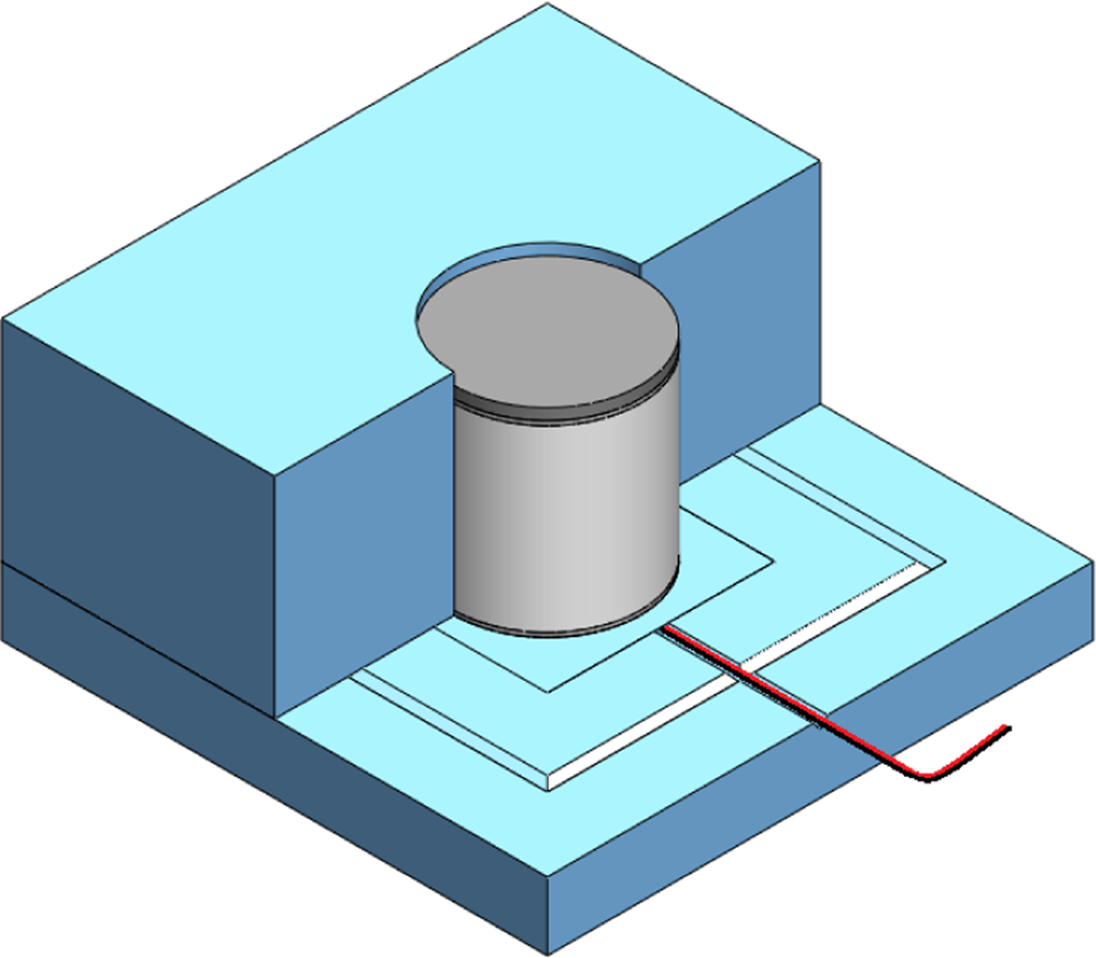
To decrease the chance that heat could escape out the sides of the firn samples, the cylindrical cavity of the insulated shell was coated with a layer of reflective foil tape. Along a square boundary outside of the heater's dimensions, a triangular cut was made into the base polystyrene square, and those triangular prisms were then hot-glued to the bottom of the lowest of the three polystyrene squares with the cylindrical cut-out. This insulated barrier aids in preventing heat loss to the cold room from between the base and the upper part of the insulated shell. To accommodate the wiring from the heater and the bottom heat flux and thermocouple sensors, a small channel was etched into the base square, providing a route for the wires to sit. A model of the custom guarded hot plate is shown in Figure 1.
Model of custom guarded hot plate design, with part of the insulative shell removed to reveal firn sample and disks.
Acrylic plates directly above and below the firn sample were used to mount the sensors, and an aluminum heat sink plate was located directly above the top acrylic plate and below the bottom acrylic plate. Hukseflux FHF02 heat flux sensors with embedded type-T thermocouples were mounted to the acrylic plates. These sensors have a sensing area of 3 cm × 3 cm and were centrally located at the ends of the firn samples, whose diameters were 10.4 cm. Aluminum-6061 was selected for the temperature distribution plate because of its high thermal conductivity, providing a rapid transfer of heat between the sample and either the cold room environment or the heater. Dow Corning 340 heat sink compound was applied between the acrylic plates and the sensors and between the sensors and the firn samples to reduce the presence of air gaps that could distort the measurements. A Minco HR6937 silicone rubber heater was chosen due to its ability to function accurately at temperatures down to − 45°C. A cross-sectional diagram of the device is shown in Figure 2.
Cross-sectional side view of the custom guarded hot plate, with sensors and parts labelled; the blue background represents the insulative shell.

3.4. Data collection and device verification
The guarded hot plate and the firn samples were stored in a cold room at − 25°C, and both the device and each firn sample were at thermal equilibrium at that temperature before each test began. The sensors and heater were connected to a Campbell Scientific CR1000 data logger, which recorded sensor data at one second intervals. The heater produced a temperature difference of 2 − 3°C across the firn samples; in general, this depended on the density of the sample: the denser the sample, the smaller the resulting temperature gradient. These temperature differences correlate to temperature gradients of 20 − 30 K m-1. No apparent thermal flux was induced by phase change during the tests; the samples’ masses were equal before and after each test, indicating that the mass was not sublimating, and there was neither melt nor any visual indications of phase change. Each test was run until the firn sample's effective thermal conductivity measurement reached steady-state, which took between 5 and 7 h. Reaching steady-state was determined both by visual inspection of the plotted data and by ensuring that the final 1000 seconds of recorded effective thermal conductivity data had a standard deviation ≤ 0.004 W m-1 K-1. Those 1000 sensor data points were averaged to produce the final effective thermal conductivity value for each sample's test.
To ensure accuracy of the built device, materials of known thermal conductivity were tested at − 25°C. Testing the custom device on materials of known thermal conductivity would verify that the device is functioning properly. To select materials whose conductivities bound the hypothesized values of firn, estimates of thermal diffusivities from values from Clemens-Sewall and others (pers. comm. 2021) were used. Those estimates indicated that the thermal conductivity of near-surface firn at the South Pole would be ~0.545 W m-1 K-1. Two test materials were chosen to bound this estimation: plasticine clay and paraffin wax, with thermal conductivities of 0.80 and 0.30 W m-1 K-1, respectively. Three tests were conducted with each material of known thermal conductivity to test the accuracy of the device; the results are shown in Table 3.
Results of verification tests using materials of known thermal conductivity

In previous verification tests of devices used to measure the thermal conductivity of snow or firn, plasticine and paraffin are both materials that researchers have implemented for this process (e.g., Pinzer and Schneebeli, Reference Pinzer and Schneebeli2009; Riche and Schneebeli, Reference Riche and Schneebeli2013). Moreover, since the guarded hot plate measures the effective thermal conductivity of a bulk sample, it is less dependent on local microstructure variations than the needle probe method. Comparatively, the needle probe method, which has been shown to be less reliable in brittle materials, such as firn and snow (Riche and Schneebeli, Reference Riche and Schneebeli2010, Reference Riche and Schneebeli2013), is often calibrated in glycerol (e.g., Sturm and Johnson, Reference Sturm and Johnson1992; Singh, Reference Singh1999; Aggarwal and others, Reference Aggarwal, Negi and Satyawali2009), a liquid substance with a drastically different material structure than snow or firn. Thus, the materials of known thermal conductivity that we selected can confidently be used to verify the accuracy of the guarded hot plate.
The total device error can be calculated using Eqn (4):

where E q is the heat flux sensor error ((± 0.05 × q) W m-2), E ΔT is the thermocouple error (± 0.05°C) and E h is the caliper error (± 0.02 mm). Using estimations of k = 0.545 W m-1 K-1, q = 10 W m-2, ΔT = 3.5°C and h = 100 mm, the total error of the guarded hot plate can be estimated as E k ≈ ±0.0283 W m-1 K-1. This theoretical margin of error is very small: at around only 5% of the estimated value, it indicates that the measurements will be accurate.
3.5. Thermal diffusivity
Whereas the thermal conductivity describes the rate at which heat can travel through a material, the thermal diffusivity describes how well heat can spread through a material. The thermal diffusivity takes into account both the effective thermal conductivity as well as the effective thermal capacity of a material, the latter of which is the bulk density of the sample multiplied by its specific heat capacity. The thermal diffusivity, α, has units m2 a-1 and is defined as:

Since the effective thermal conductivity of firn is measured using the guarded hot plate, the associated thermal diffusivities of the firn samples can be calculated from those measurements using Eqn (5). As the thermal diffusivity is more directly applicable in ice-sheet modeling, these results will be presented in addition to the effective thermal conductivity measurements.
4. Results and discussion
4.1. Effective thermal conductivity measurements
Each of the ten firn samples were measured five times, producing 50 total measurements of the firn core's effective thermal conductivity at varying depths. The direct effective thermal conductivity measurements range from 0.454 to 1.090 W m-1 K-1, and the average standard deviation of each sample's measurements is 0.031 W m-1 K-1. Our measurements show that the effective thermal conductivity of firn increases with increased depth and with increased density. The results of these tests are shown in Table 4 and are plotted with respect to depth in Figure 3. The results with respect to density are plotted in the subsequent section (see Fig. 5) as part of the comparison between this study's thermal conductivity measurements and those from previous studies.
Effective thermal conductivity measurements as a function of depth, with the average value for each sample shown and bars of one standard deviation.

Individual measurements of the effective thermal conductivities of firn samples, including the average and standard deviation for each sample

The variability in repeated measurements of the same sample is attributed to differences in its placement in the guarded hot plate. Repeat measurements involved the removal of the sample from the device, followed by the subsequent replacement of the sample into the device later in the same orientation; the variation in measurements may be attributed to the granularity of the firn on a small scale, so that the specific grains of ice that contact the plates of the guarded hot plate may change with each placement of the sample. Because of this variance, it is expected that the heat travels through the firn sample in slightly different ways with each test, resulting in the spread of data within each sample. There is no distinct trend over the course of each sample's testing, rather the small increases and decreases in the measured thermal conductivities are random. A typical time-evolution of the thermocouples, heat flux sensors and instantaneous calculation of the effective thermal conductivity for a firn sample in the guarded hot plate is shown in Figure 4. It can be seen that the variation between repeated measurements of any sample is much smaller than the variation of thermal conductivity between different samples.
Typical time evolution of sensor data.

The effective thermal conductivity calculations reach steady-state before the individual sensors, as shown in Figure 4. Once the effective thermal conductivity measurement reaches steady-state, this value does not change during the time it takes for the sensors to also reach steady-state, which allows for a shorter testing period for each measurement without compromising accuracy.
4.2. Estimations based on firn and snow
Our measurements can be compared to the existing firn measurements and estimations from previous studies. In Figure 5, our measurements are plotted along with estimates from other studies described above. There is agreement between our measurements and those of previous studies; specifically, our measurements align well with measurements at − 20°C of Calonne and others (Reference Calonne2019), Giese and Hawley (Reference Giese and Hawley2015) and Clemens-Sewall and others (pers. comm. 2021). The measurements of Marchenko and others (Reference Marchenko2019) are widely scattered, though our measurements fall centrally within the scatter.
Comparison of the effective thermal conductivity measurements to measurements and estimations from other studies. The bulk thermal diffusivity data point from Giese and Hawley (Reference Giese and Hawley2015) produces an estimated thermal conductivity value of 0.479 W m-1 K-1 using Eqn (5) based on their provided firn core density and an estimated specific heat capacity. Similarly, the bulk thermal diffusivity value from Clemens–Sewall and others (pers. com. 2021) is estimated at 0.545 W m-1 K-1.

This study's data can also be compared to the equations based on seasonal snow that have been used in the past to estimate the thermal conductivity of firn, as listed in Table 1. In Figure 6, those equations are plotted against our measurements. To compare the existing estimation equations to our thermal conductivity measurements, the Euclidean norm has been implemented. The Schwerdtfeger (Reference Schwerdtfeger1963) and Van Dusen (Reference Van Dusen1929) equations, which are often used as the upper- and lower-bounds of firn's thermal conductivity, respectively (Cuffey and Paterson, Reference Cuffey and Paterson2010), were shown to also bound our measurements. The equation of Sturm and others (Reference Sturm, Holmgren, König and Morris1997), which is based on a large data set of seasonal snow measurements, largely underestimates the thermal conductivity of firn, with a norm of 0.736 W m-1 K-1. The equation of Sturm and others (Reference Sturm, Holmgren, König and Morris1997) should not be used for modeling firn. The equation of Calonne and others (Reference Calonne2019) does not accurately capture the curve of the distribution of our data with a norm of 0.437 W m-1 K-1. The equation of Yen (Reference Yen1981) is closest to our measured thermal conductivities, with a norm of 0.273 W m-1 K-1, followed by that of Calonne and others (Reference Calonne2011), with a norm of 0.306 W m-1 K-1. Although these equations are both underestimations of our measurements, the curves of both equations align with our data's distribution. The Euclidean norms of each equation compared in Figure 6 are shown in Table 5.
Comparison of the measured effective thermal conductivities of firn to the existing equations based on seasonal snow used to estimate k and its bounds as a function of density. Equation (6) is shown in the limited density range of 350–700 kg m-3.

Euclidean norms of the estimation equations compared to our measurements

4.3. Thermal diffusivity measurements
Using our measured thermal conductivity data, the thermal diffusivities of firn can be calculated using Eqn (5). These calculations produce individual measurements that range from 19.0 to 28.5 m2 a-1, with the average standard deviation of each sample's measurements being 0.99 m2 a-1. Given the dependence of thermal diffusivity on thermal conductivity, it follows that the thermal diffusivity of the measured firn samples also increase with increased depth and with increased density. The complete results of these calculations are provided in Table 6.
Individual measurements of the thermal diffusivities of firn samples, including the average and standard deviation for each sample

As described above, Clemens-Sewall and others (pers. comm. 2021) estimated that the bulk thermal diffusivity for near-surface firn at South Pole is 18.3 m2 a-1 with a corresponding density of 429 kg m-3. Giese and Hawley (Reference Giese and Hawley2015) estimated that for the top 30 m of firn at Summit Station, Greenland, the bulk thermal diffusivity is 25 ± 3 m2 a-1 with a corresponding density of 425 kg m-3. Since the estimation of Giese and Hawley (Reference Giese and Hawley2015) comes from a different site than that of both Clemens-Sewall and others (pers. comm. 2021) and this study, it is more suitable to compare these thermal diffusivity data points with respect to density, not depth, in Figure 7.
Thermal diffusivities of firn as a function of density. The data from this study is shown as the average value for each sample, with the bars representing one standard deviation of the sample measurements. The data point of Giese and Hawley (Reference Giese and Hawley2015) is shown along with bars representing the uncertainty of that estimation.

The thermal diffusivity estimation of Giese and Hawley (Reference Giese and Hawley2015) is higher than those from this study with similar densities. This difference could be due to a variety of factors. For example, the firn samples are from sites with different accumulation patterns, which could result in different firn microstructures that have similar densities. Additionally, in-situ measurements are prone to environmental processes, such as windpumping, which the firn samples in this study were not exposed to, as they were tested in-lab. The estimation from Clemens-Sewall and others (pers. comm. 2021) comes from a site near South Pole, and it estimates a lower thermal diffusivity than those from this study with similar densities. Both Giese and Hawley (Reference Giese and Hawley2015) and Clemens-Sewall and others (pers. comm. 2021) use an indirect approach for estimating the thermal diffusivity of firn based on matching modeled temperature profiles to ones measured in-situ, which results in estimations; those are not direct thermal conductivity measurements.
4.4. Recommended equations for the effective thermal conductivity of firn in ice-sheet modeling and remote-sensing applications
Based on our effective thermal conductivity measurements of the firn samples, two equations have been fit to the data: one as a function of firn density and one as a function of firn depth. An exponential curve was selected for the density-dependent equation since, in addition to accurately fitting the measured data, it additionally provides an optimal end-behavior at the density of ice:

Inputting the density of ice into Eqn (6), the predicted thermal conductivity is k firn(ρ ice) = 2.4 W m-1 K-1, which is the known thermal conductivity of ice at − 25°C.
An exponential curve was similarly selected for implementation in the depth-dependent equation:

In this case, since direct measurements were taken on samples up to 4 m in depth, the end-behavior for small depths is known to be appropriate, as the equation fits the data. For deeper samples, the equation predicts that at depths of around 100 − 110 m, the effective thermal conductivity is that of solid ice; this range of depth is appropriate for estimating at what point the firn transforms into glacial ice when compared to the known range at South Pole, which is between 115 and 121 m, thus this equation also demonstrates its robustness (Battle and others, Reference Battle1996). Equation (6) has an adjusted R 2 of 0.919 and Eqn (7) has an adjusted R 2 of 0.896.
These formulas offer remote-sensing analysts and ice-sheet modelers new equations that are based on direct firn measurements down to a depth of 48 m. Because the formulas allow the effective thermal conductivity of firn to be estimated using either the firn's density or depth, there is additional flexibility in the application of the equations, depending on the available firn data or modeling need. For ice-sheet and regional climate modeling, where estimations of the thermal conductivity of firn are needed, these equations are recommended. For temperatures of firn other than − 25°C, the simple multiplicative factor $k_i/k_i^{{\rm ref}}$ is recommended for both Eqns (6)–(7), where k i is the known thermal conductivity of ice at the target temperature and $k_i^{{\rm ref}}$
 is that at − 25°C, such as investigated in Calonne and others (Reference Calonne2019).
5. Conclusion
We have presented the first direct measurements of the effective thermal conductivity of polar firn down to a depth of 48 m, based on firn samples from the East Antarctic Ice Sheet at the South Pole. The measurements show an increase in effective thermal conductivity with increased density and with increased depth. While existing equations for estimating the thermal conductivity of firn are unable to capture both the values and the curve of the distribution of our measurements, our measurements of the thermal conductivity fit within the spread of data from previous studies. For use in ice-sheet modeling or interpretation of remotely sensed data, Eqns (6) and (7) are recommended, which are based on the direct measurements of the thermal conductivity of firn presented in this study.
Although there are strong density- and depth-dependencies among the thermal conductivity of firn, some firn samples whose porosities or densities were vastly different from one another were found to have similar thermal conductivities. To better understand the relationship between firn structure and its effective thermal conductivity, the microstructural properties of firn samples will be investigated in ongoing research on co-located samples with thermal conductivity measurements. Additionally, the guarded hot plate will be used in future studies using samples from different sites on the Greenland and Antarctic Ice Sheets for comparison with the equations presented here.
Acknowledgements
We thank Sergey Marchenko for promptly providing his data set of thermal conductivity estimations from Lomonosovfanna, Svalbard. We thank the National Science Foundation for enabling this research through grants NSF-OPP 1443341 and 2024163. This research was supported by funding to S.O. by the Kaminsky Undergraduate Research Award and the Kanoff Family Fund for Undergraduate Research in Engineering and Science at Dartmouth College. We thank the US Ice Drilling Program for support activities through NSF-OPP 1836328.


 Open access