

1 Introduction
“There are two times in a man’s life when he should not speculate. When he can’t afford it, and when he can.” Mark Twain, Pudd’nhead Wilson’s New Calendar, 1897
Speculative gambling is risky business. While Mark Twain counsels against investment bets, no matter what, his words admit that people’s changing fortunes often have a bearing on what they decide to do.
Understanding how prior gains and losses affect risk attitudes is a significant question in the study of intertemporal choice. Research in this field has produced various perplexing results. Some experimental studies suggest that individuals often become more willing to gamble following gains (Reference Thaler and JohnsonThaler & Johnson, 1990). Other studies propose either that individuals become more risk-seeking after losses (Reference Langer and WeberLanger & Weber, 2008) or, the opposite, more risk-averse (Reference Shiv, Loewenstein, Bechara, Damasio and DamasioShiv et al., 2005; Reference Liu, Tsai, Wang and ZhuLiu et al., 2010).Footnote 1 Here, we investigate the degree to which the experience of gains and losses influences subsequent asset allocation choices made by a sample of clients of an Italian private bank. Thus, we look at the risk behavior of real-world investors, the paper gains or losses in their portfolios, and their monthly asset allocation changes during the year 2015.Footnote 2
As it happens, supervisory authorities in Italy and elsewhere require banks and other financial intermediaries to identify the risk profile of each client — commonly on a scale that runs between “no-risk” and “risk-seeking”. The level of hazard assumed by an investor’s portfolio is supposed to correspond to his or her risk profile. This is why financial service firms assess a value-at-risk (VaR) measure which determines the maximum amount of potential loss and its probability within a specific time frame. Banks and financial intermediaries gather information about clients through forms approved by supervisory authorities. The questionnaires list demographic and financial characteristics such as age, gender, level of education, work experience, financial knowledge and wealth. These characteristics determine the level of VaR that is suitable for a given investor.Footnote 3 Banks and financial intermediaries must check whether the VaR of a particular portfolio matches its owner’s risk profile. The portfolio VaR fluctuates over time as an investor modifies his or her asset allocation, but it can never be allowed to exceed the investor’s VaR.
We examine monthly asset allocation changes made by clients of an Italian private bank. The bank in question considers six levels of VaR: 0 represents “no-risk”; 1, “low-risk”; 2, “prudent balanced risk”; 3, “balanced risk”; 4, “aggressive balanced risk”; and 5 “high-risk”. The greater the loss a specific investor is able to tolerate, the higher the VaR is permitted to be. To repeat, VaR itself assesses the level of risk of the portfolio. This aspect of our study is noteworthy since — as far as we know, without exception — past empirical research on investor trading assesses only the risks and returns associated with individual transactions.
Portfolio allocation decisions are often altered by an investor’s advisor (see, e.g., Reference Foerster, Linnainmaa, Melzer and PreviteroFoerster et al., 2017). Evidently, the fact that advisors guide investors makes it difficult to interpret the findings of an analysis like the one already outlined. That is why we opt for a much smaller sample comprised only of investors who act on their own (i.e., without experienced advisors) and who all qualify for the highest level of VaR.
Our paper contributes to the literature on dynamic choice under risk and uncertainty. How do past gains and/or losses influence the level of downside risk assumed by investors? Section 2 summarizes past research and “what we know” about risk behavior. Sections 3 presents our data collection effort. Section 4 presents the main hypothesis and the methods that are used. Section 5 discusses the results. Section 6 concludes.
2 Theory and literature
A central feature of prospect theory and its successor, cumulative prospect theory, is that people are not consistently risk-averse (Reference Kahneman and TverskyKahneman & Tversky, 1979; Reference Tversky and KahnemanTversky & Kahneman, 1981; Reference Tversky and KahnemanTversky & Kahneman, 1992). Rather, people are risk-seeking in the domain of losses and risk-averse in the domain of gains, with gains and losses defined relative to a target or reference point. Also, individuals feel the pain of a loss more acutely than the pleasure of an equal-sized gain. These basic insights are corroborated by many experimental studies of risky decision making.Footnote 4 Kahneman even dismisses as a “myth” the widespread belief among finance experts that the task of an advisor is to find a portfolio that fits the investor’s attitude to risk. The fundamental problem with individual risk tolerance, Kahneman submits, is that “there is no such thing” (2009, p. 1).Footnote 5
Reference Thaler and JohnsonThaler and Johnson (1990) demonstrate that people tend to assume higher risk immediately following a previous gain. This psychological tendency is labeled the house money effect. It is supported by the further laboratory experiments of Reference Battalio, Kagel and JiranyakulBattalio et al. (1990), Reference Keasey and MoonKeasey and Moon (1996), and Reference Ackert, Charupat, Church and DeavesAckert et al. (2006). Reference Franken, Georgieva, Muris and DijksterhuisFranken et al. (2006) study the Iowa Gambling Task of Reference Bechara, Tranel and DamasioBechara et al. (2000), which involves repeated choices among four decks of cards, two of which have negative expected value because they lead to large but infrequent losses. Young adults who experienced gains make more gainful and safer choices afterward than people who were subjected to losses. Then again, in an adaptation of Franken et al., Reference Rosi, Cavallini, Gamboz and RussoRosi et al. (2016) find that previous episodes makes no difference. As mentioned, Reference ImasImas (2016) shows that many individuals with paper losses accept more risk but that, once a loss is realized, they take less risk. Imas also replicates selected findings of Reference Shiv, Loewenstein and BecharaShiv et al. (2005), Reference Weber and ZuchelWeber and Zuchel (2005), and Reference Langer and WeberLanger and Weber (2008).
Besides theory and laboratory-type experiments, there is limited empirical evidence. However, Reference Malmendier and NagelMalmendier and Nagel (2011) and Reference Bucciol and ZarriBucciol and Zarri (2015) look at the long-lasting effects on risk attitudes of traumatic experiences such as the Great Depression. Weber et al. (2012) use repeated surveys of British investors to study their risk taking during (and closely after) the 2008 financial crisis. Reference Frino, Grant and JohnstoneFrino et al. (2008) consider the behavior of futures traders in Australia. Reference Liu, Tsai, Wang and ZhuLiu et al. (2010) look at market-makers in the Taiwan Futures Exchange. Gains earned during morning hours appear to produce above average risk-taking during afternoon trading. In addition, Reference Hsu and ChowHsu and Chow (2013) study individual investors in Taiwan. After substantial gains, investors assume greater risks. Hsu and Chow notice that, as time goes by, the house money effect slowly weakens. Lastly, Reference Lien and ZhengLien and Zheng (2015) look at slot machinge gambling.Footnote 6
Clearly, it is difficult to tell what defines a gain or loss for a specific investor or to predict frames (Reference FischhoffFischhoff, 1983; Reference BarberisBarberis, 2013). For instance, investors may consider gains and losses in overall wealth, or in the value of their securities, or in the value of a certain asset. If we focus on a specific stock, a return that is positive may be considered a gain, or a return that exceeds the risk-free rate. Timing poses a further problem. Does the investor fixate on weekly, monthly, annual or lifetime gains and losses? This is the problem of choice bracketing Broad bracketing, which allows people to con¬sider all the consequences of their actions, often leads to superior decisions (Reference Read, Lowenstein and RabinRead et al., 1999).
Numerous studies attempt to connect risk preferences with demographic factors such as age, gender and education.Footnote 7 As a rule, risk tolerance strengthens with a higher level of schooling, e.g., a university education (Reference Riley and ChowRiley & Chow, 1992; Reference Halek and EisenhauerHalek & Eisenhauer, 2001; Reference Hartog, Ferrer-i-Carbonell and JonkerHartog et al., 2002; Reference Dwyer, Gilkeson and ListDwyer et al., 2002).
Generally, women are more risk-averse (e.g., Reference Bajtelsmit and BernasekBajtelsmit & Bernasek, 1996; Reference Powell and AnsicPowell & Ansic, 1997; Reference Byrnes, Miller and SchaferByrnes et al., 1999; Reference Schubert, Brown, Gysler and BrachingerSchubert et al., 1999; Reference Eckel and GrossmanEckel & Grossman, 2008; Reference Lusardi and MitchellLusardi & Mitchell, 2008; Reference Croson and GneezyCroson & Gneezy, 2009) while men are more overconfident than women (e.g., Reference Barber and OdeanBarber & Odean, 2000; Reference Croson and GneezyCroson & Gneezy, 2009; Reference Eckel and GrossmanEckel & Grossman, 2008).
With respect to age, the evidence is more ambiguous. For example, Reference Mikels and ReedMikels and Reed (2009), Reference Nielsen, Knutson and CarstensenNielsen et al. (2008), and Reference Albert and DuffyAlbert and Duffy (2012) find that, compared to young adults, the elderly are more risk-averse for losses. Reference Lauriola and LevinLauriola and Levin (2001), and Reference Weller, Levin and DenburgWeller et al. (2011) indicate that the same is true for gains. On the other hand, Reference Mather, Mazar, Gorlick, Lighthall, Burgeno, Schoeke and ArielyMather et al. (2012) suggest that aging instigates risk-seeking in the domain of losses, and Reference Samanez-Larkin, Gibbs, Khanna, Nilsen, Carstensen and KnutsonSamanez-Larkin et al. (2007) and Reference Thomas and MillarThomas and Millar (2012) find no link, either for losses or gains, between risk attitudes and growing older. If measured by the ratio of risky assets to total wealth, risk tolerance may rise with age (Reference Wang and HannaWang & Hanna, 1997). Regarding the link between age and the fraction of equity in investment portfolios (“the risky share”), there is no consensus.Footnote 8
As a final point, we note that past gains and losses may also guide financial decisions for the reason that they change people’s beliefs, e.g., about their power to generate precise return forecasts or to control risk. Reference Moore and HealyMoore & Healy (2008) discuss various aspects of overconfidence. The experiments of Reference Nosić and WeberNosić & Weber (2010) imply that poor calibration encourages aggressive risk-taking. Reference MerkleMerkle (2017) reports related empirical findings.Footnote 9 Clearly, outcomes that validate a person’s beliefs or actions elevate confidence. People may fantasize that success primarily reflects personal ability. Self-assessments of competence correlate with self-assurance (Reference Graham, Campbell and HaiGraham et al., 2009). That many people hold inflated views of themselves, and are also unaware of it (Reference Kruger and DunningKruger & Dunning (1999).
3 Data
A private bank provided us with access to data. We are not allowed to disclose its name, but we can reveal that the bank is located in Northern Italy and that it is one of the five market leaders in financial planning, operating across Italy through a network of more than 1,000 financial advisers. As shown on http://www.assoreti.it, the website of the Associazione delle Società per la Consulenza agli Investimenti, the customers of banks such as ours typically have portfolios invested primarily, if not exclusively, in mutual funds, managed portfolios, insurance and pension funds. A fraction of clients, about 1 percent, use a part of their portfolio, usually between 5% and 10%, for direct investment in shares and/or bonds. With reference to this portion of the portfolio, managed autonomously, some clients adopt a buy-and-hold approach, i.e., they buy securities and hold them over extended periods of time. Others perform trading operations.
We created a data set using several criteria. First, we only consider investors with a total portfolio at the bank worth, on average, about €300,000 and with a portfolio that has two parts. The first piece, representing roughly 90% of its value, is administered with the supervision of a personal financial adviser. The second piece, corresponding to roughly 10%, is managed by the investor on his/her own via home banking. We label this part the “trading portfolio”. It is the main object of our study. Second, we study investors’ asset allocation decisions related to their trading portfolios during the calendar year 2015. In particular, we analyze data for clients who adjust their trading portfolios — at least once a month — but do not refashion the overall strategy of the total portfolio during 2015. This element is essential since, in some cases, financial advisers suggest specific asset allocation modifications, and clients may well apply the advice to their trading portfolios. To repeat, in order to be able to observe portfolio revisions made by clients in complete autonomy, we include only investors who never alter the asset allocation of the total portfolio under management but who do modify the trading portfolio.
Third, we exclude bank clients who add or withdraw funds (say, for consumption purposes) from their trading portfolio between January and December 2015. This makes it much easier for them to calculate and to mentally grasp monthly percentage returns and monetary gains or losses (in Euro).
Finally, we exclude clients who, for whatever reason, are not permitted by bank rules and procedures to raise their portfolio VaR into category 5, i.e., the maximum. Overall, our panel data set comprises data for 62 investors. For each, we have statistics regarding age, gender, level of education, the value of the trading portfolio, monthly gains and losses, and variations in portfolio risk exposure, i.e., the private bank’s estimates of the VaR of the trading portfolio. Our data are snapshots of portfolio value and VaR at the end of each month between January and December 2015.Footnote 10 We note that the subjects in the sample have access to the same information and, of course, much more. On a bank website, they can inspect the composition of their trading portfolio, the account balance, and the VaR at any time, and as often as they wish. (The VaR is calculated around-the-clock.)Footnote 11
4 Hypothesis and Methods
Monthly changes in VaR are the dependent variable in the analysis that follows. In effect, we pretend that, at every month’s end, each individual subject faces a “decision point” where the performance of the trading portfolio over the most recent month is evaluated. At that time, the investor may resolve to vigorously correct the strategy. Only substantial adjustments would lead to a category change in VaR that becomes detectible, straightaway, over the current month. The main predictors of ΔVaR that we employ below are either a gain/loss dummy variable for changes in value of the trading portfolio during the prior month (priorGLD) (gain=1) or the percentage portfolio return (multiplied by 100) for the prior month (priorRET).
To be fully clear, consider an investor who at the beginning of month #1 has a trading portfolio of €100 (V1) invested in stocks and bonds with a VaR equal to 3. During the month, the investor performs at least one transaction that may modify the asset allocation within the trading portfolio and may produce a gain or a loss. Imagine that at the end of month #1 (which is also the start of month #2), the trading portfolio asset allocation is changed in terms of stocks and bonds so as to achieve a VaR equal to 4 and the value of the portfolio value is now €110 (V2). In this example, the investor obtains a gain of V2−V1 and records an increase in VaR from 3 to 4, so that the ΔVaR is +1. See Figure 1.
Overview of the data and the hypothesis.

The main hypothesis tested below is that paper investment gains that are earned over an initial period embolden individuals to accept more risk during a later period. Conversely, current paper losses cause people to diminish risk afterward. We check whether changes in the VaR-category of the trading portfolio during month t (ΔVaR) are predicted by investor-specific portfolio gains or losses during month t − 1.Footnote 12
At first glance, the hypothesis appears to challenge prospect theory since we propose that achievement promotes adventure and failure invites prudence. This is false. We relate present changes in risk behavior (observed through fluctuations in VaR) to past returns. The time dynamics are key. Vis-à-vis decision-making under risk, not only future risk and return matter to investors, but so does history.
Our customized data set and empirical methods intend to reproduce a natural experiment, i.e., a study in which nature, i.e., factors outside our control, exposes clusters of individuals to dissimilar experimental and control conditions. Importantly, the process that governs exposures resembles random assignment. To repeat, we have access to portfolio values and VaRs at the end of each month between January and December 2015. This makes 62 investors ×11 months = 682 observations of ΔVaR, priorGLD, and priorRET. Since we relate changes in risk to prior month returns, the first set of 62 ΔVaRs that may be analyzed are for March 2015. The last set is for December 2015. All in all, we are able to examine investor behavior at 620 decision points which occur at the end of February 2015 through the end of November 2015 as subjects come to grips with the monthly performance of their trading portfolios.Footnote 13
Since we have panel data, we estimate random-effects ordered logit regressions with changes in portfolio risk levels (ΔVaR) as a categorical dependent variable.Footnote 14 Age, gender, education, and the total value of the trading portfolio at the end of the previous month serve as control variables. The main regression is:
Likewise, we run the same regression with priorGLD substituting for priorRET. We also conduct a string of robustness tests.
5 Results
The main result is that, as hypothesized, the subjects become more risk-averse after suffering losses and more risk-seeking after experiencing gains, from month to month. Relevant details for this result are in Section 5.2. Section 5.1 provides basic descriptive statistics.
5.1 Descriptive statistics
Tables 1, 2 and 3 offer descriptive statistics for 62 private bank clients. Hereafter, we briefly state — and further illustrate — the main facts in these tables.
The mean VaR across 682 monthly observations was 2.90. The 2015 age of the individuals in the sample varied between 35 and 65 years. On average, the subjects were 47 years old. Sixteen (26%) were women; 44% were university-educated. (Women were equally distributed between education levels.)
The mean trading portfolio balance, across investors and months, was €30,952. The minimum was €20,204 (investor #14, female, with a high-school education, age 55, and an average monthly VaR of 2.00) while the maximum was €46,125 (#25, male, high-school educated, 57, VaR 3.00).
The largest recorded loss in portfolio value between January and December 2015 was €13,000 (an 11-month return of −38.2% for #37, male, high-school educated, 41, VaR 2.92); the largest recorded gain came to €9,000 (a return of 32.1% for #33, female, university-educated, 40, VaR 2.42). The median investor lost €150.
Panel B in Table 1 shows data similar to panel A but for subsamples arranged by age, gender, education, and the monthly average trading portfolio balance. On average, older investors ran portfolios with somewhat lower VaRs but the difference is not large. Compared to the men, the women in the sample managed portfolios that were about €4,000 smaller with VaRs that were much lower. (Note the t- and Mann-Whitney U-tests.) Subjects with a university degree were on average 5½ years younger than high-school graduates. Larger portfolios displayed higher VaRs.

Some of the relationships thus far discussed are also visible in Table 2, a correlation matrix.
It shows that the current monthly returns earned by individual investors (RET), these same returns for the previous month (measured either by priorRET and priorGLD, the gain/loss dummy), the VaRs and ΔVaRs are all strongly positively correlated.

Table 3 shows some of the data month-by-month.
Between January and August 2015, the average portfolio was rising in value. This was followed by big negative shocks in September and October. The same pattern emerges in the monthly VaRs, averaged across bank clients. Also, in all months but September, there were some subjects who increased the value-at-risk of their portfolios; in all months but July, some decreased VaR. About 2/3’s of all monthly observations are gains; 8% are associated with increases in ΔVaR, 7% with decreases in ΔVaR, and 85% cause no change in value-at-risk.
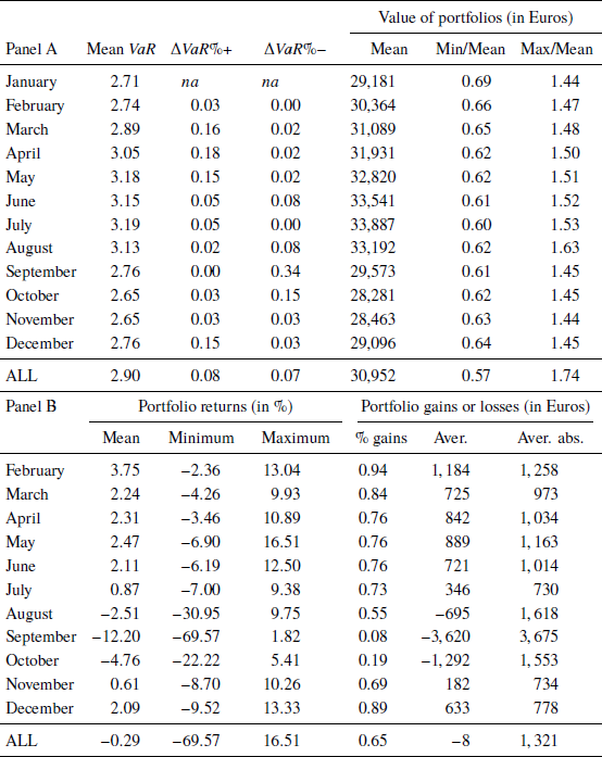
The simple average monthly portfolio return was minus 29 basis points, equivalent to a loss of €8. In terms of this investigation, the averages are deceptive, however. The absolute monthly change in portfolio value, averaged across individuals, is €1,321; the same statistic calculated for two-month periods is €2,294, and it is €3,202 for three-month periods. Figure 2 is a histogram with all one-month gains and losses for all subjects between February to November 2015. Evidently, most monthly value changes are modest, and cannot be expected to prompt changes in risk-taking, but a considerable number are very large relative to the size of the portfolio. As seen in Table 3, the cruelest monthly shock was a loss of €16,000 in September (−69.57% for #28, female, 41, high-school educated, VaR 2.83); the best result was a gain of €7,100 in May (+16.51% for #1, male, 35, university-educated, VaR 4.50).
Trading portfolio gains or losses in Euro (62 investors, 10 decision points each, February-November 2015).
5.2 Tallying VaR transitions and regression evidence
In a simple analysis, we regressed the change in VaR category on whether the previous month showed a gain or a loss, for each subject. Of the regression coefficients, 39 were positive, 2 were negative, and 21 were 0. This difference suggests that changes of the last month affect risk taking in the present month.
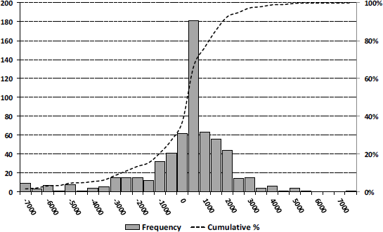
For a more complete analysis, Table 4 (panel A) presents the transition matrix describing the frequency with which investors move their portfolios from one VaR category to another.
Each cell lists the total number of cases, the number of cases associated with portfolio gains during the previous month, and the ones associated with losses during that month. Panel B shows the fraction of VaR transitions of different types, and panel C lists the matching average €gain or loss, averaged across all observations for the matrix cell.
Since the largest percentages are on the main diagonal of panel B, Table 4 indicates that investors tend to preserve the status-quo level of VaR. Values outside the diagonal and other than zero represent the changes in VaR which we want to explain. The average ΔVaR is close to zero, and this remains true even if we exclude the 85% of cases on the diagonal. Some individuals changed VaR as often as three or four times during 2015. Others never did.
The main insight derived from Table 4 is that VaR increases (from 2 to 3, from 3 to 4, and from 4 to 5) are allied with a high proportion of gains and high average €gains during the previous month. VaR decreases (from 3 to 2, from 4 to 3, and from 5 to 4) are coupled with a high proportion of losses and high average €losses.Footnote 15 This agrees with our main hypothesis.
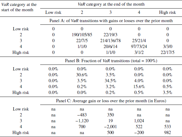
Figure 3 presents a different route to the same destination. There, all past one-month gains or losses, previously shown in Figure 2, are sorted into quintiles and, for each quintile, we find the fraction of all VaR increases and all VaR decreases associated with it. The results are crystal clear. Nearly half of all VaR decreases accompany the 20% of months with the worst portfolio performance. Also, roughly 70% of all VaR increases follow months with portfolio value changes in the top 40%. Lastly, the middle quintile shows less than proportional VaR increases and decreases. If past gains or losses did not bring about changes in risk-taking, all bars in Figure 3 should have been of the same height.
Fraction of all bank-recorded VaR increases or decreases by quantile of gains or losses over the prior month (620 decision points).
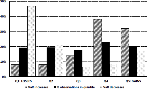
Table 5 displays the regression results for the full sample and various subsamples.
We estimate random-effect ordered logistic regressions. The dependent variable is Δ VaR. The predictor variables are Age (in years), Gender (female=1), Education (high education=1), the value of the portfolio at the beginning of the month (in thousands of Euros), a gain/loss dummy (PriorGLD, gain=1) for the change in portfolio value during the prior month, and the portfolio return during the prior month (PriorRET, in percent). The regressions are for the full sample and for subsamples. *** is p<.01; **, p<.05; *, p<.10. S.E., clustered by individual investor, are in parentheses.
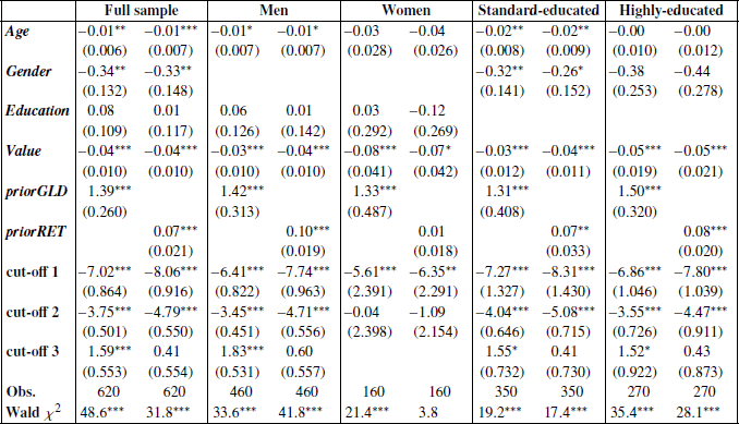
The cut-off points in the table are auxiliary parameters that separate the four categories of the dependent variable (ΔVaR) is +1, 0, −1, or −2). Equality tests strongly reject the null hypothesis that the cut-off points are equal — confirming the relevance of the four categories. For the sample as a whole, the results indicate that, except for education, all variables contribute in a significant way. The results are fairly uniform across subsamples.Footnote 16 Older subjects are less likely to appear in the top category, i.e., their risk appetite is lower. The same applies to women, and to clients with somewhat more abundant portfolios.
6 Conclusion
In the financial industry, and also in finance theory, the assessment of investor risk profiles is normally seen as a elementary step toward identifying asset portfolios that are most appropriate to serve client needs. Past studies find that risk tolerance varies with demographic factors that change slowly over time or not at all. Here, we offer direct evidence that risk preferences and/or beliefs about one’s ability to manage risk and return evolve from month to month and in direct response to recent portfolio performance. This is shown for a sample of genuine investors who act on their own without external advisory influence. All told, fast-changing circumstances predict fast-changing risk attitudes.
If correct and characteristic of the behavior of important segments of the financial community, our empirical findings appear to offer some circuitous support for modern asset pricing theory in the manner of Reference Campbell and CochraneCampbell and Cochrane (1999) and others. The fact that we study active traders likely helps to explain why our results are so markedly different from the inertia reported by Reference Brunnermeier and NagelBrunnermeier and Nagel (2008) who, based on data from the Panel of Income Dynamics, report that most U.S. households do not adjust the share of their portfolios invested in risky assets following wealth changes, and who find in favor of constant relative risk aversion.Footnote 17
Our chief result, however, is that, for the Italian bank clients in our sample, past portfolio performance — which, as we have seen, can be quite erratic — predicts short-term variations in risk-taking quantified by value at risk. The house money effect of Reference Thaler and JohnsonThaler and Johnson (1990) is not discarded by our data set, and neither is the alternate view that fluctuations in self-confidence, feeding an illusion of control, is the main culprit. However, the tests do appear to challenge Reference ImasImas (2016).
The investors that we study are amateurs, not experts. Our analysis agrees with the Dunning-Kruger effect (Reference Kruger and DunningKruger & Dunning, 1999). Intuitively, it is plausible that amateurs look at past performance, even if not realized, to divine the future, especially when they act alone without highly trained assistance. Success builds confidence; failure undermines it.Footnote 18 The switches from less risk tolerance to more, and vice versa, on the basis of near past performance also lead us straightforwardly to Bandura’s concept of self-efficacy. The beliefs that people hold about their capabilities, e.g., the presence or lack of mastery, affect the quality of their functioning. Self-efficacy has a bearing on thought patterns, emotional arousal, and behavior (Reference BanduraBandura, 1982). The findings in this article suggest to us that quite a few investors (i) may eventually come to doubt their own skills, (ii) may no longer put in much effort, and (iii) do not truly learn from experience. As their self-efficacy erodes, they may have a sense of futility, perhaps apathy.Footnote 19 Of course, we recognize that these last sentences are highly speculative, and necessitate much more investigation. The results may also have some limited practical/regulatory use. Italian banks and financial intermediaries are required to monitor the level of risk of their clients’ portfolios so as to avoid excessive loss exposure and potential discontent. Financial advisers who observe unusual trading and fluctuations in risk-taking may use our findings for didactic purposes, leading clients to be more sensible in their investments and thereby also building more fruitful advisory relationships.


 Open access