Introduction

Ogives are transverse surface features that form at the rate of one per year at ice falls on some alpine glaciers. Ogives travel down-glacier at the surface velocity of the ice, so that the wavelength of an ogive pattern is the distance ice flows in one year. There are two related types of ogives: pairs of alternating light and coloured bands, called “Forbes bands”, first described by Reference Forbes, Edinburgh and BlackForbes (1843), and topographic waves called “wave ogives”. Not all wave trains on glaciers are wave ogives. Trains of serac blocks formed in ice falls can cause wave patterns down-stream (Reference TyndallTyndall, 1874, p. 180; Reference WashburnWashburn, 1935; Reference FisherFisher, 1947; Reference SharpSharp, 1960; Reference VallonVallon, unpublished), and compressive stress gradients can cause wave trains distinct from wave ogives (Reference HoldsworthHoldsworth, 1969; Reference HughesHughes, 1971, Reference Hughes1975; Reference WilliamsWilliams, 1979). Ogives occur in many parts of the world, e.g. the Alps (Reference Forbes, Edinburgh and BlackForbes, 1843), Norway (Reference King and LewisKing and Lewis, 1961), Iceland (Reference Ives and KingIves and King, 1954; Reference King and IvesKing and Ives, 1956), Greenland (Reference AthertonAtherton, 1963), the Canadian Rockies (Reference SherzerSherzer, 1907, p. 50), the Andes (Reference LliboutryLliboutry, 1957, Reference Lliboutry1958), the Karakoram (Reference Yafeng and WenyingYafeng and Wenying, 1980), the Himalaya (Reference HaefeliHaefeli, 1957), and Alaska (Reference LeightonLeighton, 1951).

Reference King and LewisKing and Lewis (1961) described the origins of the coloured bands. In their view, crevasses near the top of Odinsbreen ice fall on Austerdalsbreen, Norway, collect dust in summer and snow in winter. Years later, when these closed and compressed crevasses are below the ice fall, they are seen as narrow structural bands (1–100 cm thick) of dirty and bubbly ice, respectively, extending to a large depth in the glacier. The Forbes bands are the result of variations in the numbers of these narrow structural bands per unit distance down the glacier. Reference LeightonLeighton (1951), Reference LliboutryLliboutry (1957), Reference FisherFisher (1951, Reference Fisher1962), Reference VallonVallon (unpublished), Reference ReynaudReynaud (1979), and Reference Lliboutry and ReynaudLliboutry and Reynaud (1981) discussed the foliated structure of ogives. The view that the banded structure is sedimentary in origin (Reference AgassizAgassiz, 1840, p. 40; Reference VareschiVareschi, 1942; Reference FisherFisher, 1947; Reference GodwinGodwin, 1949) is now largely discredited.

It has long been known that there is some connection between wave ogives and Forbes bands. Reference TyndallTyndall (1874, p. 131) and Reference King and LewisKing and Lewis (1961) associated the dark bands with the troughs of the wave ogives and the light bands with the crests. Reference AthertonAtherton (1963) and Reference EllistonElliston (1957), who worked in a variety of different climatic regions, associated the dark bands with the leading slopes of the waves.

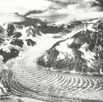
Typical wave ogives may have a crest-to-trough amplitude of 10 m right below the ice fall. The amplitude usually decays with distance travelled down the glacier, so that often only 10–20 waves are seen. Differential mass balance due to snow drifts in the troughs (Reference NyeNye, 1958; Reference LickLick, 1970) and, possibly, viscous relaxation of the waves (Reference GlenGlen, 1958; Reference VallonVallon, unpublished) reduce the wave amplitude, these processes usually dominate the wave amplification caused by longitudinal compression down-glacier from the ice fall. Some wave-ogive trains persist, however, for many more years, e.g. Trimble Glacier North Branch, Alaska Range (Fig. 1).

Fig. 1.

Wave ogives on Trimble Glacier, Alaska. (Photograph by A.S. Post; U.S.G.S. Project Office-Glaciology negative # F654-94.)

Early theories of ogive-wave formation (Reference Forbes, Edinburgh and BlackForbes, 1843; Reference HaefeliHaefeli, 1951[a], Reference Haefeli[b], Reference Haefeli1957; Reference Streiff-BeckerStreiff-Becker, 1952) favoured a seasonally varying longitudinal stress at the foot of the ice fall; these variations were assumed to be caused by seasonal changes in the sliding velocity. From strain observations on Austerdalsbreen, however, Reference NyeNye (1959[a], Reference Nye[b]) calculated the distribution of stress and found that the ogives there could not be explained by seasonal pressure changes. Reference NyeNye (1958) proposed another mechanism for creating wave ogives. He showed that, even when the flow was steady, annual waves should be expected below an ice fall, due to interaction between the annually periodic seasonal mass balance and the large plastic deformations taking place in the ice fall. A vertical column of ice passing through an ice fall in summer is stretched horizontally by the local high velocity gradients, thus exposing a larger surface area than ice columns of equal volume immediately above and below the ice fall. This ice in the ice fall in summer loses a larger fraction of its volume to ablation, becoming a trough in an ogive-wave train down-glacier from the ice fall. Reference VallonVallon (unpublished, p. 51) applied Nye’s theory to the generation of ogives from Séracs du Géant on the Mer de Glace. Reference MartinMartin (1977) showed that this mechanism could also generate kinematic waves at ice falls in response to fluctuations of climate. The Nye theory is the basis of the developments reported here. Reference WashburnWashburn (1935) also suggested that the annual mass-balance cycle could cause wave ogives but he did not attempt to formulate the principle mathematically.

Large seasonal variations in velocity exist on many glaciers and these seasonal changes may well cause additional annual waves. However, to quote Reference NyeNye (1958), “If the waves from an icefall are thought to be due entirely to some other process, it is then necessary to explain why the ablation mechanism is absent.” Because the mechanism described by Nye is capable of generating large annual waves that adequately explain observed wave ogives, I will restrict further attention to the simple case of steady ice flow. The existence of waves caused by unsteady flow merits attention but is not examined here.

Quantitative Treatment

Let x be the coordinate in the direction of ice flow and U(x) be the forward velocity of the ice. Because the theory concerns regions of thin and rapidly sliding ice, U(x) is approximately equal to the ice-surface velocity.

Since the wavelength of wave ogives where they become visible below an ice fall rapidly becomes less than the ice thickness (due to compressive flow), the wave forms are too short to propagate as kinematic waves (Reference Langdon and RaymondLangdon and Raymond, 1978) (Reference NyeNye (1958) discussed this possibility), and the waves do not perturb the flow. This is consistent with the assumption that U(x) is independent of time, i.e. ∂U/∂t = 0. The waves are simply carried forward at the velocity of the ice surface, which is treated strictly as a “conveyor belt” in this theory. Letting h(x, t) be ice thickness, Nye defined an Annually Repeating State (ARS) by h(x, t) = h(x, t + 1) for time in years. W(x) is the transverse width between two flow lines, A(x, t) the mass-balance rate, and Q(x, t) the ice flux given by

Following a section of ice moving at U(x) in channel of unit width, Nye used the steady-velocity assumption to convert the continuity equation

to the total derivative form

Odinsbreen ice fall at Austerdalsbreen is in the ablation zone. Nye assumed that the amount of winter snowfall there was unimportant to the wave-generation process, being merely a protective covering for the true glacier surface. To simplify the analysis, he also assumed that the net annual ablation of ice occurred instantaneously each year at time t ₀, i.e.

where δ(t) is the Dirac delta function, n is an integer, and b(x) is the net annual balance given by

He then derived a recursion relation for the glacier-thickness profile h(x) in an ARS immediately after the ablation at t ₀

for ice that was at position (x – λ) one year previously. Nye assumed a constant input ice thickness of 13.8 m at the origin x = 0 for Odinsbreen ice fall and used Equation (6) to predict the wave pattern at Austerdalsbreen (Fig. 2c). The annual mass balance b(x) and the surface velocity U(x) shown in Figure 2a are redrawn from Reference NyeNye (1958).

Fig. 2.

(a) Austerdalsbreen velocity and mass balance. Odinsbreen ice fall; curves redrawn from Reference NyeNye (1958). T(x) is the time in years for ice to flow from the origin to position x. (b) Wave-excitation potential for W = 1 m. Arrows indicate approximately linear sections in Table I. (c) Austerdalsbreen ice thickness h(T) at the midpoint of the ablation season. Solid curve: numerical solution with 3 months ablation season. Broken curve: Reference NyeNye (1958) with instantaneous ablation.

The agreement was good between the observed and predicted wavelength and phase. The theory does not attempt to predict the decay of the waves. The sharpness of the troughs resulted from the unrealistic assumption in Equation (4); the ablation season at Austerdalsbreen actually lasts about 3 months (Reference NyeNye, 1958).

Wave ogives have been reported in accumulation areas (Reference AthertonAtherton, 1963; Reference Post and LaChapellePost and LaChapelle, 1971, p. 57). Although Nye formulated the theory in terms of instantaneous ablation, the same combination of seasonal mass balance and plastic deformation can produce waves above the firn line.

The ablation-plastic deformation mechanism is capable of producing very large waves at ice falls anywhere on a glacier. The question that arises (e.g. Reference Post and LaChapellePost and LaChapelle, 1971, p. 57) is: why are large ogives not present below many active ice falls?

Wave-Ogive Solution Characteristics Using Method of Characteristics

The continuity Equation (2) with steady velocity U(x) can be solved in a more general form that includes the wave ogives caused by the mechanism Nye described, and explains the absence of waves below many ice falls.

Multiplying the continuity Equation (2) by U(x) and by W(x), and using Equation (1) gives

Now, I change the distance variable x to a new variable T(x) the time required for ice to flow from the origin (x = 0) to position x. T and x are related by

Nye also used this transformation when evaluating Equation (6). T will be treated as the independent space variable with the understanding that for any spatially varying function f, f(T) ≡ f(x(T)).

Using the chain rule with Equations (8) gives

so that Equation (7) becomes

This equation is readily solved by the method of characteristics (e.g. Reference WhithamWhitham, 1974, p. 19) to give

along the characteristic curves dT/dt = 1, i.e. along T = t – ϕ where ϕ is an integration constant.

These characteristics (Fig. 3) are the trajectories of the vertical ice columns. Each characteristic is labelled by a unique value of ϕ, the time when that ice passed the origin.

Fig. 3.

Characteristics in (T, t) space. T(x) is the time taken by ice to flow from the origin to x, so it measures position on the glacier, and t is time. Each characteristic, representing the trajectory of an ice column, is parameterized by ϕ, the time the ice passed the origin T = 0.

Equation (11) is a single total derivative in one spatial variable T. It resembles Equation (3) used by Nye and is easily integrated to give

where T ₀ is a reference position at which the boundary condition is applied.

To represent wave ogives, the solution in Equation (12) must contain terms that correspond to wave forms travelling down the glacier at the speed of the ice, i.e, at 1 year’s flow distance per year. This requires the form Q(t–T). Below the ice fall, this propagating solution must also have a spatial periodicity of 1 year’s flow distance.

To proceed further, I will assume that the mass balance A(T, t) is separable into the summation

This form includes, as a special case,

where the annual cycle Y(t) is weighted by the annual net balance x(T) at each position T. The mass balance in Equation (4) that Nye used for Austerdalsbreen had this form. Because Equation (12) is linear in the mass balance, the summation in Equation (13) will carry through all the linear operations which follow. To keep the expressions as simple as possible, I can consider the case N = 1, and drop the subscripts, without loss of generality.

It is possible to introduce travelling wave forms into the solution through propagating mass-balance waves having the form A(T, t) = b(t – T) when N is larger than unity in Equation (13). In fact, the disappearance of the wave ogives can be represented by such terms; zones of excessive ablation rate propagate down the glacier so as to remain on wave crests. I have not included this effect in the examples 1 show. Any propagating waves formed between T ₀ and T in the examples arise from the ablation-stretching mechanism.

It will be useful, subsequently, to define a function B(t) as an integral of the temporal variation Y(t) of the mass balance

To simplify the appearance of the equations, I will define a “wave-ogive excitation potential” ψ(T)

which comprises the total spatial dependence of the integrand in Equation (12), The gradient of this potential will be the forcing function for wave ogives.

The input flux at the up-stream boundary T = T ₀ is used as a boundary condition. Substituting the mass balance in Equation (14) into the continuity Equation (10) evaluated at the boundary T ₀, gives

Integrating this from time zero to time t = T ₀ + ϕ i.e. up the vertical boundary line at T ₀ in the (T, t) plane (Fig. 3) using Equation (15), gives

This is the input flux at the boundary T ₀ for the characteristic ϕ. There are three terms. The first is a constant datum flux equal to the flux that crossed the boundary T ₀ at time t = 0. The second term is the change in flux at the boundary due to the synchronous rise and fall B(t) of the whole surface in response to the seasonal changes. The final term gives the flux changes at the boundary T ₀ due to advection of spatial wave forms through the boundary.

Substituting the mass balance in Equation (14) into the flux solution of Equation (12) using the excitation potential in Equation (16), and recalling that y(t) = dB/dt, gives

Integrating by parts on the right-hand side,

After substituting the boundary condition Equation (18), and setting T + ϕ = t,

If the summation is carried through from Equation (13),

To find the waves in the ice-thickness profile h(T, t), divide through by U(x(T))W(x(T)), To see the waves as a function of distance x rather than the travel time T, stretch the T axis by the inverse transformation in Equation (8). Equation (22) is the solution for the flux at all times t and positions T > T ₀ with the assumptions:

• (1) velocity is steady everywhere, and

• (2) mass balance is separable as in Equation (13).

The first three terms in Equation (21) were discussed above. The final term, defined as P(T ₀ T,[t -T]), yields the wave ogives. The dependence on [t–T] indicates that this term contains a disturbance propagating in the positive x direction at the same speed as the ice.

To represent wave ogives, it must also be an ARS. Because the seasonal balance variation Y(t) has a period of 1 year, so does its integral B(t) (Equation (15)), provided that the mean of Y(t) is made zero by a suitable choice of the terms in Equation (13); then substituting B(t) = B(t+1) into the propagation term P yields P(T ₀ ,T,[t – T]) = P(T ₀,T,[t+1-T]), i.e. the wave form is an ARS. Furthermore, for T in a region below the ice fall where the forcing function dψ/dT vanishes, P(T ₀,T + l[t -T + 1]) = P(T ₀,T,[t – T]), i.e. the propagating disturbance is a wave that repeats with a wavelength of 1 year’s flow distance.

Linear Systems Formulation for Ogives

Implications

I will consider two types of driving functions, and use the convolution Equation (24) to illustrate how destructive interference can occur, even on active ice falls, to prevent the formation of observable waves. Combinations of these simple velocity patterns can be applied to any ice fall to get a convenient estimate of the expected ogive-wave amplitude.

Austerdalsbreen

Reference King and LewisKing and Lewis (1961) attributed the Forbes bands on Austerdalsbreen to seasonal differences in dust accumulation, melting, and snow accumulation in the crevasses formed in the upper part of the Odinsbre ice fall, where the ice undergoes a longitudinal extension. This region is between x = 500 m and x = 1000 m in Figure 2. Since wave ogives are often associated with Forbes bands, it is interesting to see which sections of the Odinsbre ice fall are most important for forming the waves.

If I assume that the width variations are unimportant (Reference NyeNye (1958) also assumed this), then, multiplying the curve U(x) by b(x) (Fig. 2a), and using the transformation in Equation (8), gives the excitation potential ψ(T) for unit width on Odinsbreen (Fig. 2b). This curve can be approximated by four sections of constant gradient. Table I gives the relative wave-amplitude function M(τ) for each section. Although Equation (29) is exact only for the mass balance in Equation (26), other annually varying mass-balance functions would show similar dependence of wave amplitude on τ. Table I suggests that the largest contribution to the generation of the waves comes from the initial section of the ice fall as the ice accelerates to maximum speed. This is the same section that Reference King and LewisKing and Lewis (1961) identified as the region responsible for the formation of the Forbes bands.

Table I.

Odinsbreen Excitation Potential ψ Approximated by Linear Sections. The end Points are Shown by Arrows on Figure 2b. W = 1 m, M(τ) is Given By Equation (29). M(0) for Section 1 is Used to Normalize All Sections

To test this idea, I have used the Odinsbre ice-fall profile (Fig. 2a) to solve the continuity Equation (10) with the numerical model from Reference WaddingtonWaddington (unpublished). The up-stream boundary condition was satisfied by a constant input flux using Reference NyeNye’s (1958) values of ice thickness (h = 13.8 m) and ice velocity (U = 1375 m a^-1). (For Nye’s model of Austerdalsbreen, the input flux was constant in time because the mass balance at the top of the ice fall was zero.)

Because the finite-difference model cannot accurately represent an instantaneous mass balance of the form in Equation (4), I used a constant ablation rate for 3 months each year. This is a more realistic representation of the Austerdalsbre mass balance (Reference NyeNye, 1958). Figure 10a shows the computed ice flux Q(T, t). Figure 10b shows the transformation to ice thickness h(x, t). The amplification of the wave height due to compressive flow is apparent. The solid curve in Figure 2c shows the ice-thickness profile h(T) in the middle of the ablation season. For comparison, the broken line is the wave pattern found by Nye using an instantaneous ablation season. The longer ablation season smooths out the sharp troughs on the waves.

Fig. 10.

Austerdalsbreen wave ogives. The numerical solution using the excitation potential in Figure 2b. with constant input flux at T = 0 and a 3 month constant ablation season. Profiles at 1.5 month intervals. T is a measure of distance down-glacier and t is time, (a) Ice flux Q(T, t); (b) Ice thickness h(x, t).

To test whether the steep gradient of ψ(T) in the upper ice fall causes the wave ogives, I then used the numerical model with two modified forcing functions. To generate the annual repeating state in Figure 11a, I brought the ice into the ice fall already travelling rapidly to give constant excitation potential of –5500 m³ a^-2, i.e. on the dotted horizontal curve AC in Figure 2b. Then I let the ice slow down following the observed Odinsbre potential curve (cd). The up-stream boundary condition in Equation (18) for this model is time-dependent, because ψ(0) is no longer zero. The waves generated in this model have only 15-20% of the amplitude of those in Figure 10a. The prediction in Table I was 15%.

Fig. 11.

Isolating the wave-generating region on Odinsbreen ice fall. T is a measure of distance down-glacier, and t is time, (a) ice follows the excitation potential acd in Figure 2b, i.e. no acceleration as it enters the ice fall. The wave amplitude is small, (b) Ice follows bce in Figure 2b. i.e. no deceleration as it leaves the ice fall. The wave amplitude is comparable to that in Figure 10a. Thus the interval over which the ice speeds up (x = 500–1000 m) is largely responsible for the wave ogives.

Next, I used the standard Odinsbre excitation potential (solid line bc) up to the peak. Then I let the ice leave the ice fall and travel down Austerdalsbreen without slowing down (dashed horizontal line ce). The flux decreases rapidly down-glacier because the ice remains thin, and ablation takes a larger proportion of the mass each year. In fact, the ice thickness becomes zero at T = 4 year, but 1 continued the simulation to negative depths to show the waves clearly. The amplitude of the waves (Fig. 11b) is approximately 80% of the amplitude in Figure 10a. The prediction in Table I was 76%. The rapid velocity increase in the upper region of Odinsbreen causes the waves, and the subsequent deceleration of the ice merely amplifies the wave height by compressive flow. It appears that the rapid extension, that is responsible for the Forbes bands, is also responsible for the formation of wave ogives.

The velocity and ablation data for Séracs du Géant in Reference VallonVallon (unpublished, p. 52) suggest that the deceleration phase at Mer de Glace also contributes very little to the wave ogives on that glacier.

Conclusions

The ablation–plastic stretching mechanism of Reference NyeNye (1958) has been extended by using the method of characteristics to solve the continuity equation. The total wave-ogive pattern on a glacier can be written as a convolution of a spatial term, the velocity-width-mass-balance gradient (forcing function), with a temporal term, the cumulative mass balance. The convolution describes their interaction.

The forcing function can be viewed as a spatial filter applied to the annually periodic mass balance. Wave ogives appear in the filter output (the glacier-flux profile) only if the filter does not heavily attenuate the annual periodic component. The theory predicts that magnitude and spatial extent of velocity changes in an ice fall modulate the amplitude of the resulting wave ogives. The modulation factor may go to zero.

Since small annual waves may go unnoticed, or be rapidly obliterated by differential ablation, this modulation may explain why some ice falls with rapid ice velocities and large annual balance variations do not generate observable wave ogives by the ablation-stretching mechanism.

Several points of physical interest can also be made:

• 1. Longitudinal variation of ice velocity, channel width, and mass balance all can generate annual waves in the same way. The waves due to velocity changes are usually the largest.

• 2. Every incremental change with x of any of these three factors generates a wave train down-glacier. This annually periodic wave train is the Green’s function for the total wave pattern.

• 3. Waves are not observed on all glaciers, because the velocity gradients are small, and waves generated over a large spatial range tend to be out of phase and to interfere destructively.

• 4. Only large and localized gradients traversed by the ice in 6 months or less can generate waves sufficiently coherent to form large wave ogives.

• 5. Wave ogives and Forbes bands are often found together, because, while the physical processes causing them are different, they both depend on the occurrence of a short zone of rapid ice acceleration, such as the upper stretch of some ice falls.