


1. Introduction
Many networks have been shown to be the result of several generations (and types) of fractures (e.g., Hancock, Reference Hancock1985; Hanks et al., Reference Hanks, Wallace, Atkinson, Brinton, Bui, Jensen and Lorenz2004; Nortje et al., Reference Nortje, Oliver, Blenkinsop, Keys, McLellan, Oxenburgh, Fagereng, Toy and Rowland2011). We term these superposed fracture networks. The characterization and description of such networks require careful identification of different types and generations of fractures. Measurement and statistical analysis can and should be designed to recognize these differences and avoid confusing and grouping of disparate structures. In this paper, we discuss how fracture types and generations can be incorporated into the geometrical and topological analysis of a network, as opposed to the analysis of individual fractures.
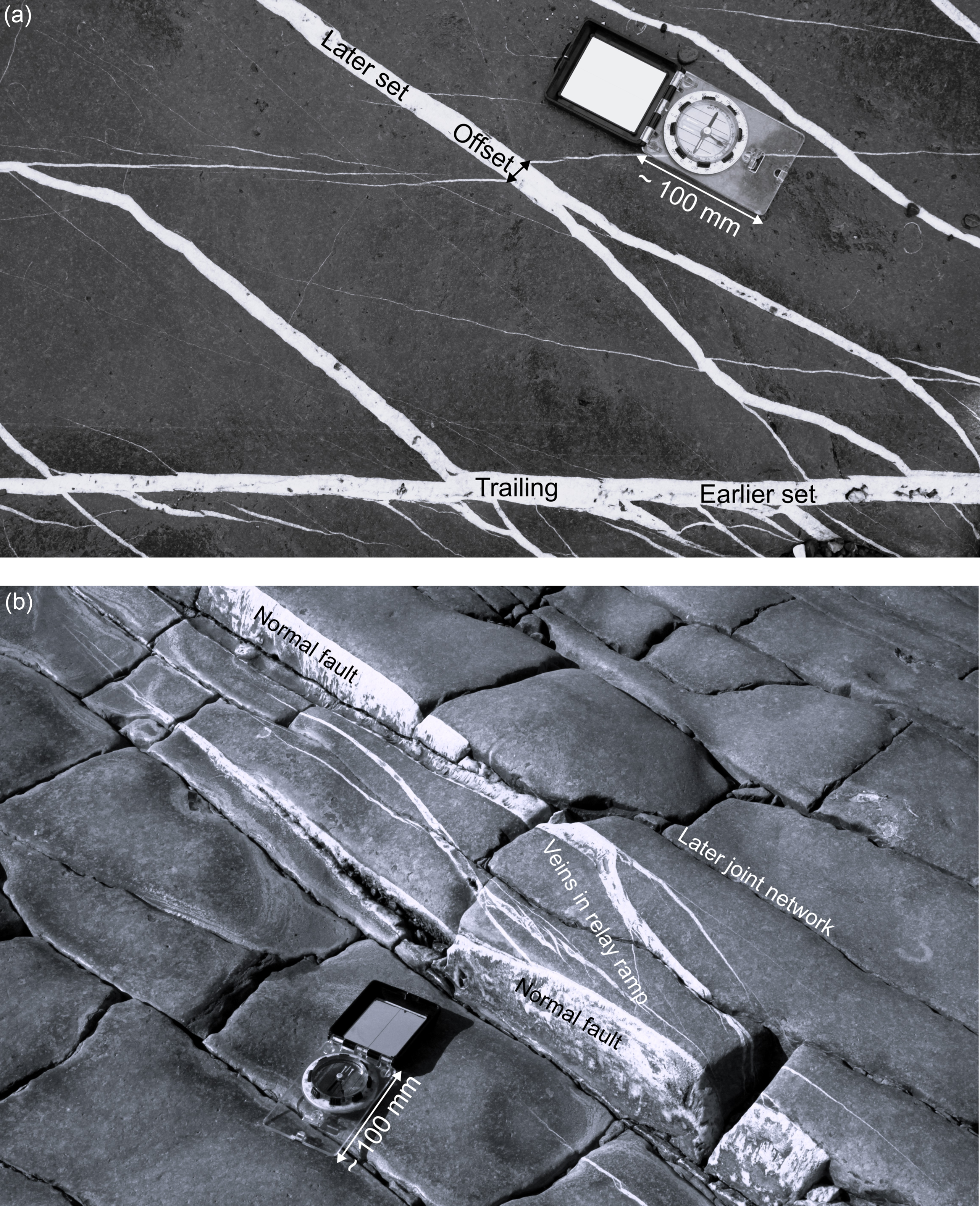
A superposed fracture network is defined here as a system that consists of more than one generation of intersecting fractures. The component fractures could be the same type, such as one set of veins that abuts, crosses or reactivates an earlier set of veins (Fig. 1a). A superposed fracture network may also include different types of fractures, such as a fault with a network of veins in a damage zone (one generation of fractures) superposed by a network of later joints (Fig. 1b). The fractures forming a component part of a superposed fracture network may either be a simple set of fractures or a network of several fracture sets. The key feature of a superposed fracture network is that it consists of different generations of fractures, as indicated by abutting, crossing and reactivation relationships. We use the terms superposed deformation (e.g., Lindström, Reference Lindström1961; Treagus, Reference Treagus1995) and superposed folds (e.g., Weiss, Reference Weiss1959) as precedents for using the term superposed to describe fracture networks. Various authors have used the term superposed fractures (e.g., Nekrasov, Reference Nekrasov1975; Lewis et al., Reference Lewis, Couples, Tengattini, Buckman, Tudisco, Etxegarai, Viggiani and Hall2023), superposed veins (e.g., Reinhardt & Davison, Reference Reinhardt and Davison1990; d’Ars & Davy, Reference d’Ars and Davy1991) and superposed faults (e.g., Stanley, Reference Stanley1974; Gorodnitskiy et al., Reference Gorodnitskiy, Filin, Malyutin, Ivanenko and Shishkina2009). The term superimposed has also been used to describe different generations of brittle structures (e.g., Gonzalo-Guerra et al., Reference Gonzalo-Guerra, Heredia, Farias, García-Sansegundo, Martín-González, Butler, Torvela and Williams2023).
Examples of different types of superposed fracture networks. (a) Two sets of calcite veins of different ages. Liassic limestone at Lilstock. View vertically downwards. (b) Normal fault zone with a network of calcite veins in a damage zone (one generation of fractures) superposed by a network of later joints. Liassic limestone at East Quantoxhead (51°11′27′′N, 3°14′15′′W). View downwards at approximately 45° to the NW.

The aims of the paper are (1) to define and illustrate the term superposed fracture networks and (2) to show the key geometric observations necessary to understand the development of superposed fracture networks and to interpret routinely measured parameters. Such an approach is also a necessary prerequisite to subsequent tectonic, kinematic and mechanical interpretation of the fractures and to understanding how the networks may contribute to the physical and engineering properties of the rock mass. For example, connectivity of a network (e.g., Manzocchi Reference Manzocchi2002; Sanderson and Nixon, Reference Sanderson and Nixon2018) is fundamental to both the flow of fluids (Lee et al., Reference Lee, Yu and Hwung1993; Berkowitz et al., Reference Berkowitz, Bour, Davy and Odling2000) and the strength of the rock mass (e.g., Dershowitz, Reference Dershowitz1984; Odling, Reference Odling1997).
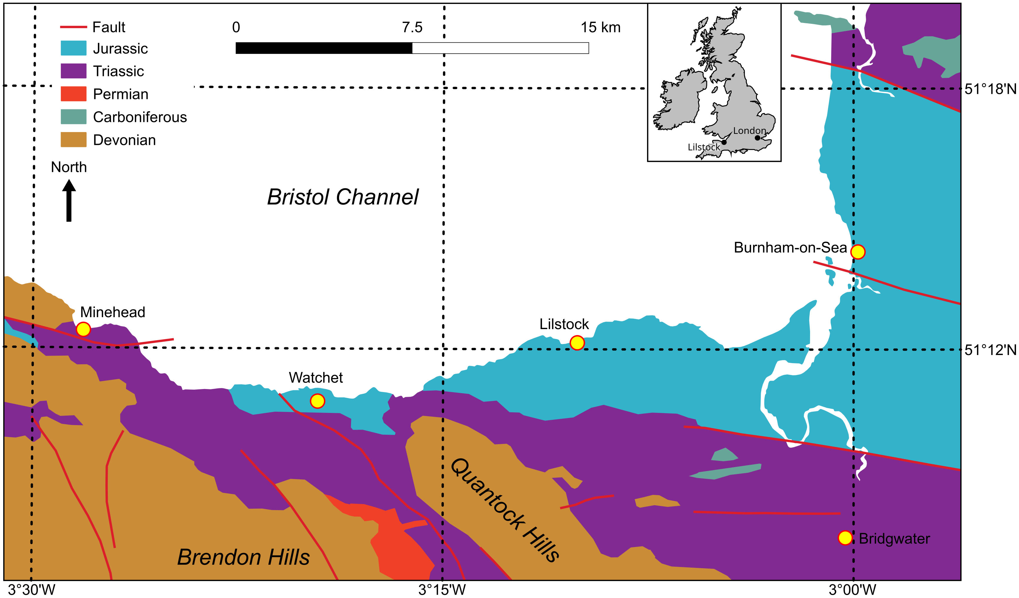
Analysis is presented of a network of veins and joints on a Liassic limestone bedding plane at Lilstock, Somerset, UK (51°12′08.9′′N 3°10′06.0′′W; Fig. 2). This location was chosen because of the high quality of the exposure and because it shows key features that enable relative ages of the network components to be determined (Peacock and Sanderson, Reference Peacock and Sanderson1999; Peacock, Reference Peacock2001). The superposed fracture networks have been mapped using drone images and GIS to record fracture type, geometry (orientation and length) and topology. This analysis is augmented with key field observations, especially at fracture intersections, to establish the sequence of fracture development. This enables the evolution of superposed fracture network to be determined.
Geological map of western Somerset, showing the location of the study site at Lilstock. The geology is from the British Geological Survey 1:625,000 scale map of the UK. Reproduced with the permission of the British Geological Survey ©NERC. All rights Reserved.

Note that here we use the noun fracture as a general term for planar brittle structures, including faults, veins and joints. More specific terms are used as appropriate. Considering brittle deformation of rock in terms of superposed fracture networks is important because the emphasis on determining the age relationships, based on geometric and topological relationships, leads to improved understanding of the development of the structures. Also note that the use of ‘younging tables’ to record relative ages of structures has been suggested (e.g., Potts & Reddy, Reference Potts and Reddy1999, Reference Potts and Reddy2000), but we do not use that approach in this paper.
2. Geological setting of the Lilstock study area
The study location is on the coast between Lilstock and Hinkley Point, Somerset, UK, on the south side of the Bristol Channel Basin (e.g., Van Hoorn, Reference Van Hoorn1987; Fig. 2). The area underwent Mesozoic N-S extension and Cenozoic N-S contraction (e.g., Dart et al., Reference Dart, McClay, Hollings, Buchanan and Buchanan1995, Glen et al., Reference Glen, Hancock and Whittaker2005). Three main groups of structures can be identified in the Liassic rocks exposed on the Somerset coast (e.g., Dart et al., Reference Dart, McClay, Hollings, Buchanan and Buchanan1995): (1) ∼095°-striking normal faults and associated calcite veins, with some of these showing evidence of both sinistral and dextral reactivation at Lilstock (Peacock & Sanderson, Reference Peacock and Sanderson1999; Rotevatn & Peacock, Reference Rotevatn and Peacock2018); (2) E-W-striking thrusts, strike-slip faults that are conjugate about ∼ N-S and reverse-reactivation of the largest 095°-striking normal faults, all with associated calcite veins; and (3) joints (e.g., Peacock, Reference Peacock2001).
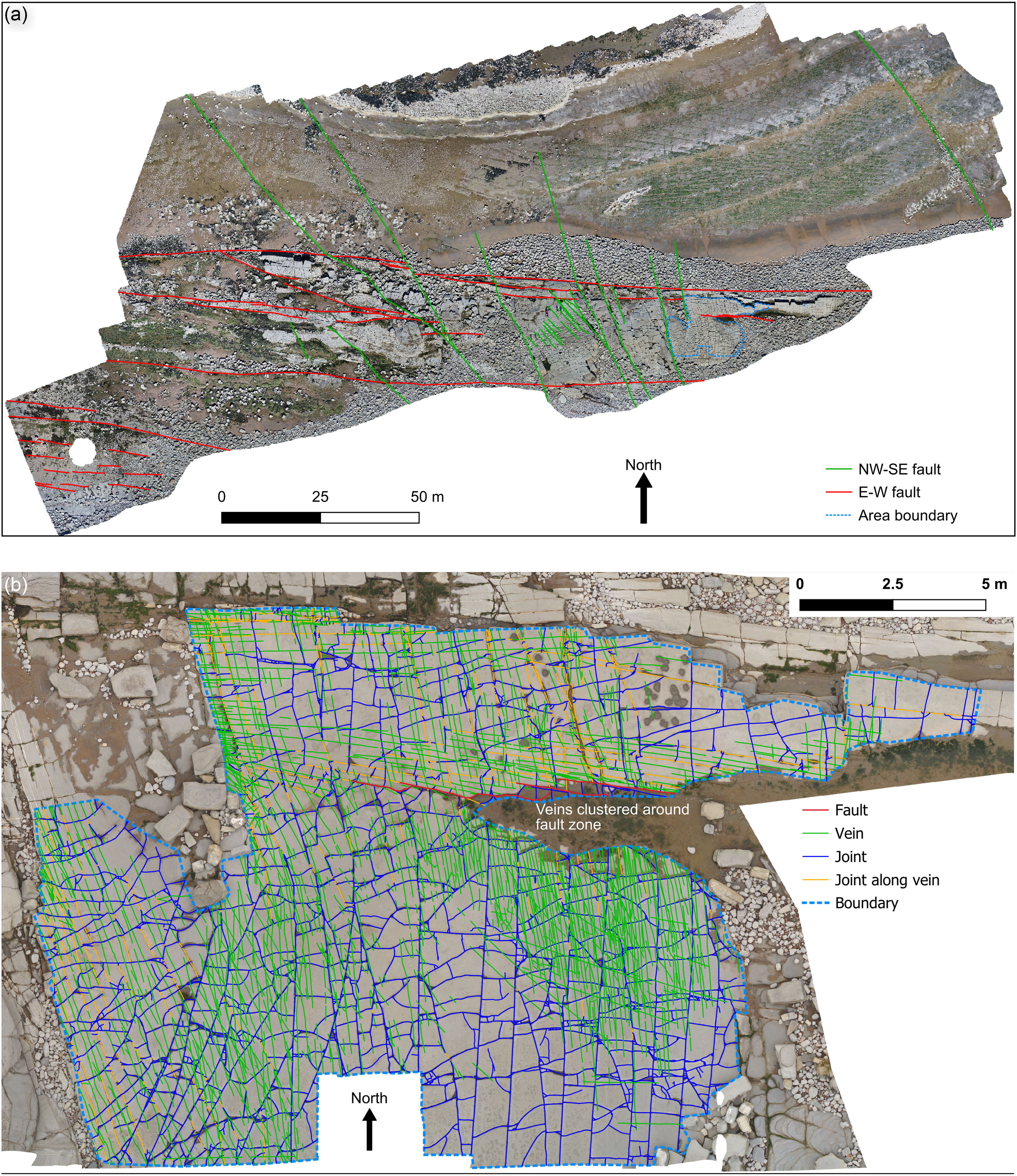
The exposure consists of a bedding plane near the base of the Liassic (Lower Jurassic) sequence of interbedded limestone and shales, approximately 0.3 m thick and dipping a few degrees to the north (Fig. 3). 095°-striking normal faults and sinistral strike-slip faults occur at the location. The vein network consists of two distinct sets formed at different times under different stress orientations. Stylolites occur between some of the en echelon veins, with shear along some stylolites causing the veins to develop as pull-aparts (Willemse et al., Reference Willemse, Peacock and Aydin1997). It is more difficult to divide the joint network into distinct sets based on their orientation, and they probably formed in an evolving stress during exhumation (Rawnsley et al., Reference Rawnsley, Peacock, Rives and Petit1998).
(a) Overview map of the area, based on an orthomosaic (pixel size ∼ 7 mm × 7 mm) made using photographs taken using a drone flown ∼20 m above the surface. Faults have been mapped from the orthomosaic, with ∼ E-W-striking faults probably having normal displacements, although some strike-slip is likely (Rotevatn & Peacock, Reference Rotevatn and Peacock2018). The ∼ NW-SE-striking faults generally show dextral displacements of up to ∼1 m. (b) Larger-scale view of the mapping area, with structures mapped from an orthomosaic (pixel size ∼ 2 mm × 2 mm).

This location was used by Ryan et al. (Reference Ryan, Lonergan and Jolly2000) to demonstrate a method for the measurement and display of fracture spacing and orientation from maps of fracture networks. A map of veins at this location was also used by Belayneh et al. (Reference Belayneh, Masihi, Matthäi and King2006) to demonstrate how a percolation approach can be used to predict vein connectivity. Willemse et al. (Reference Willemse, Peacock and Aydin1997) and Sanderson and Peacock (Reference Sanderson and Peacock2019) use examples of veins within approximately 300 m of the exposure to demonstrate aspects of vein development. Exposures on the coast, approximately 2.1 km west of the location, have been used to analyse joint patterns (e.g., Passchier et al., Reference Passchier, Passchier, Weismüller and Urai2021).
We use this location to: (1) recognize different fracture types, (2) determine the geometries and topologies of the different fracture types, (3) interpret the age relationships and development of the superposed fracture networks and (4) determine the effects of pre-existing fractures on the development of later fractures. Note that here the emphasis is on the veins and joints rather than faults and stylolites.
3. Methods
3.a. Data collection
A drone was flown at a height of ∼3 m above the exposure to collect 577 vertical photographs, each photograph being 4864 × 3648 pixels. They cover an area ∼96 m E-W and 20.6 m N-S. The flight was planned using the DroneDeploy application, with the images having ∼70% overlap to allow photogrammetry. Agisoft Metashape was used to create an orthomosaic, with each pixel being ∼ 2 mm × 2 mm, and a digital elevation model (DEM) with pixel sizes of ∼ 4 mm × 4 mm.
3.b. Mapping
The orthomosaic and DEM were analysed using QGIS (version 3.26.0). The traces of fractures were digitized at scales of up to 1:2, with the ‘enable snapping’ and ‘enable snapping on intersection’ functions switched on. The following four types of fracture trace were digitized:
-
Faults: identified by lateral displacement of pre-existing veins seen on the orthomosaic and by height differences on the bedding plane highlighted by using hill-shading of the DEM.
-
Veins: appear as white or light brown lines on the orthomosaic.
-
Joints: appear as black or dark lines on the orthomosaic.
-
Joints along veins: fracture traces that consist of both veins and joints (i.e., joints following and reactivating veins).
These classes enable analysis of all of the fractures that are veins (by combining veins and joints along veins) and of all of the fractures that are joints (by combining joints and joints along veins). The resolution of the imagery means that we only consider veins or joints with lengths greater than ∼4 mm and veins with apertures of greater than ∼2 mm.
3.c. Problems and ambiguities
Various problems and ambiguities were encountered when digitizing the fractures. While it was generally simple to identify faults with lateral offsets of a few millimetres or vertical offsets of a few centimetres, it was more difficult to identify smaller displacements. It was also difficult to accurately identify the tips of faults, where displacements decrease to sub-resolution scales, especially where such faults pass laterally into veins apparently with only opening-mode displacements. The faults are mineralized and joints tend to follow portions of those faults, but they have been mapped simply as faults.
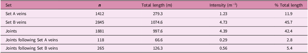
Some of the veins in the area have apertures of up to about 70 mm. The area also shows veins with centimetre-scale spacings, metre-scale lengths and sub-millimetre-scale apertures, these being formed by a process termed crack-jump by Caputo and Hancock (Reference Caputo and Hancock1998). It is therefore difficult to see the smaller veins at the resolution of the orthomosaic. See Snow (Reference Snow1970), Marrett (Reference Marrett1996) and Forstner and Laubach (Reference Forstner and Laubach2022) for descriptions of fracture apertures in rock. As with the faults, it is particularly difficult to see the low-displacement parts of the veins, making it hard to identify vein tips and therefore to determine the connectivity of the veins. Veins are typically segmented, with many veins being composites of linked segments (e.g., Vermilye & Scholz, Reference Vermilye and Scholz1995). It can be difficult to decide whether to digitize two stepping veins or a single composite vein, which may influence the numbers of traces mapped but has little effect on the sum of their lengths (Table 1). Another ambiguity is that some later veins intersect, follow and re-emerge from earlier veins. Such trailing veins were digitized as being two veins intersecting the older vein rather than as a single vein. We consider this preferable to trying to identify and digitize each case of trailing.
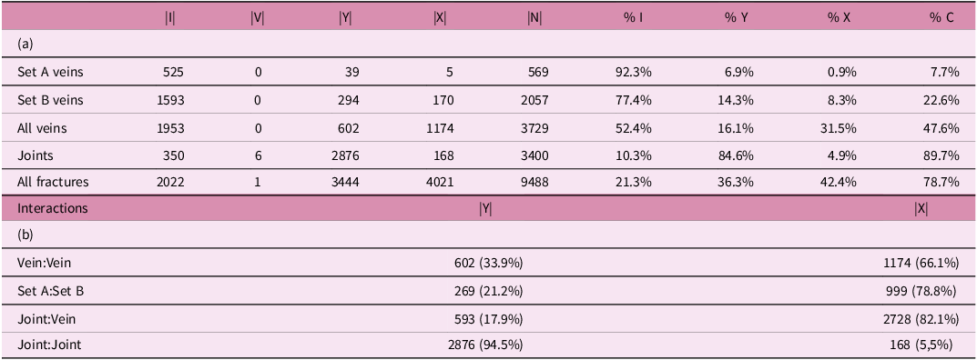
Data for fracture trace lengths for the superposed fracture network at Lilstock. Mapped area = 227.358 m2. Intensity is mean length per unit area. Note that the values for ‘Joints’ includes the values for ‘Joints following Set A veins’ and ‘Joints following Set B veins’. 6.7% of the length of joints follows Set A and 12.6% of the length of joints follows Set B. 23.8% of the length of Set A is followed by later joints, while the 11.7% of the length of Set B is followed by later joints

The imagery has a pixel size of ∼ 2 mm × 2 mm. The traces of all of the fracture types identified can form anastomosing patterns, sometimes making it difficult to determine the start and end points of each anastomosing fracture, which may influence such parameters as the length distributions of the fracture networks. These side-stepping and anastomosing patterns are mostly near or below the resolution of the imagery and are not considered in construction of the larger scale (>>4 mm) networks represented and analysed in this paper. We only consider total trace lengths for the different fracture types (Table 1) rather than their scaling relationships.
The veins have widths of up to several millimetres, and many of the joints also have mm-scale apertures, probably partly because of weathering. The intersection points (nodes) are therefore really areas rather than points, but those intersection areas are small relative to the scale of the mapping.
While these various issues created some problems with digitizing and interpretation, the ambiguous traces comprise a small percentage of the total fracture population. We consider them to not influence the main observations or results presented in this paper.
3.d. Ground-truthing
The mapping using the orthomosaic and DEM was undertaken with the benefit of numerous previous visits to the location. It was necessary, however, to ground-truth the results, check the relationships between different types and sets of fractures, and take higher-resolution photographs of key features (i.e., from nearer to the exposure than the ∼3 m height flown by the drone).
4. Relationships between superposed fractures
We identify four common types of relationships between pairs or sets of fractures of different ages, with the relationships giving information about the relative ages of the fractures (Peacock et al., Reference Peacock, Sanderson and Rotevatn2018):
-
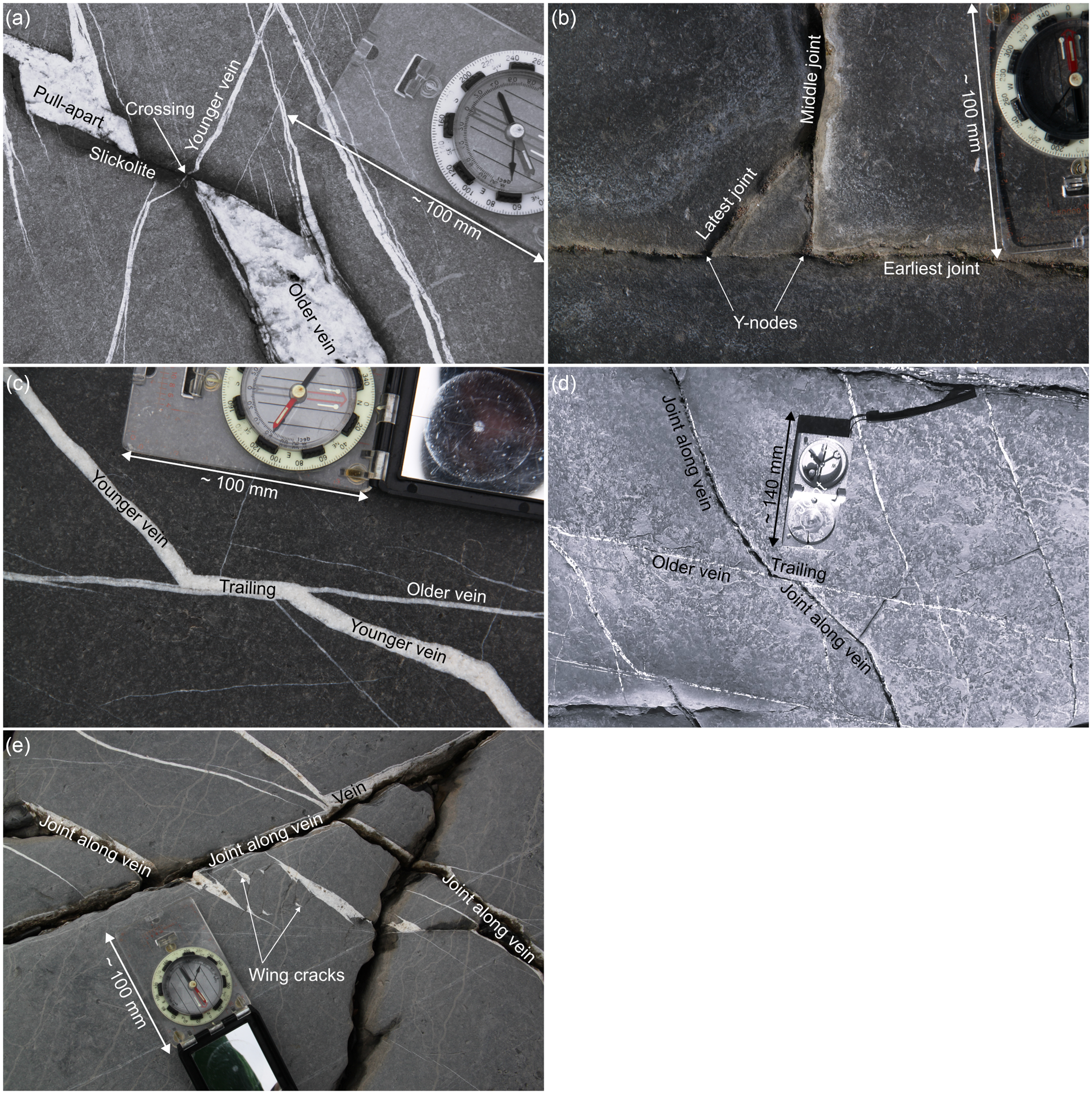
Cross-cutting: where later fractures cross and displace earlier fractures. A fault that crosses and displaces another fault will be the younger of the two (e.g., Chen, Reference Chen2013). The relative ages of crossing veins can commonly be determined by the displacement patterns (Fig. 4a) or by the pattern of mineral infills (e.g., Craw et al., Reference Craw, Upton, Yu, Horton and Chen2010). The lack of measurable displacements or mineral fill mean that it is difficult to determine the relative ages of crossing joints.
-
Abutting: where a fracture meets another fracture at an intersection line or point. A later joint commonly abuts an earlier joint (Fig. 4b; e.g., Rives et al., Reference Rives, Rawnsley and Petit1994). Note, however, that an earlier fault can be displaced by, and therefore abut, a later fault (e.g., Nixon et al., Reference Nixon, Sanderson, Dee, Bull, Humphreys and Swanson2014). Also note that abutting relationships can be caused by the splaying of one fracture off another, with the two fractures being synchronous (e.g., Biddle & Christie-Blick, Reference Biddle, Christie-Blick, Biddle and Christie-Blick1985).
-
Trailing: where two new fractures are connected through an older fracture, with renewed displacement occurring on the older fracture (Fig. 4c, d). Trailing faults are illustrated by Nixon et al. (Reference Nixon, Sanderson, Dee, Bull, Humphreys and Swanson2014), Phillips et al. (Reference Phillips, Jackson, Bell and Duffy2018) and by Deng and McClay (Reference Deng and McClay2021), and trailing veins are illustrated by Virgo et al. (Reference Virgo, Abe and Urai2013, Fig. 12c).
-
Reactivating: the term reactivation is typically used for renewed displacement on a fault that has undergone a prolonged period of inactivity (e.g., Shephard-Thorn et al., Reference Shephard-Thorn, Lake and Atitullah1972; Sibson, Reference Sibson1985). Here, however, we generalize the term for other fracture types, such as where a joint follows and causes renewed opening along an earlier vein (e.g., Fig. 4e). Such reactivation of fractures has been described for veins (e.g., Ramsay, Reference Ramsay1980; Zulauf, Reference Zulauf1993; Evans, Reference Evans1994), dykes (e.g., Drobe et al., Reference Drobe, Lindsay, Stein and Gabites2013) and faulted joints (e.g., Wilkins et al., Reference Wilkins, Gross, Wacker, Eyal and Engelder2001).
Examples from Liassic limestones at Lilstock of different types of relationships between fractures that give information about their relative ages. All views are approximately vertical downwards. (a) Earlier veins are connected by slickolites to form pull-aparts, with a later vein crossing a slickolite. (b) Abutting joints, with the abutting relationships giving the relative ages of the joints. (c) Trailing calcite veins. (d) Example of joints trailing through a calcite vein. (e) Later joints following and reactivating earlier calcite veins.

These relationships provide evidence for the relative ages and therefore the superposition of fracture networks. It may also be possible to use non-geometric data to determine superposition, such as mineral paragenesis and radiometric dating of different fracture cements (e.g., Guastoni et al., Reference Guastoni, Pennacchioni, Pozzi, Fioretti and Walter2014).
5. Geometries of superposed fracture networks at Lilstock
5.a. Vein networks
The calcite veins show the following characteristics:
-
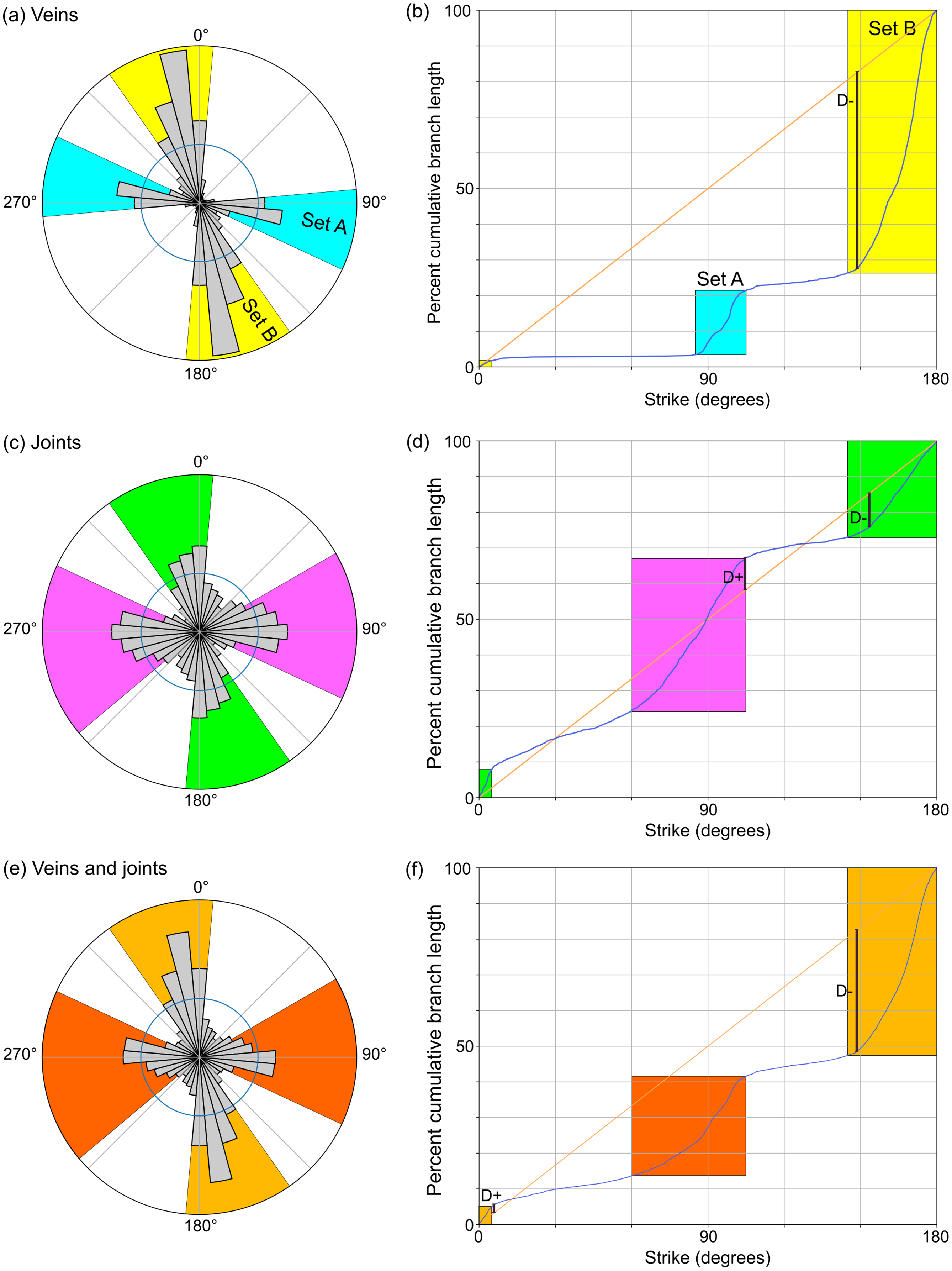
Orientations. The mapped veins all dip at ∼90° to bedding, which has a gentle dip to the north, with vein strike data shown in Fig. 5a, b. These strike data indicate two sets of veins, one set striking ∼ 085° to 115° (Set A, ∼18% of data) and another a dominant set striking ∼ 145° to 185° (Set B, ∼75.5% of data). The sets have a strong and well-defined preferred orientation, with most of the data (∼93.5% of data) within these narrow orientation ranges (Fig. 5a). These two sets have been divided in QGIS using cut-offs of 045–125° (Set A) and 125–225° (Set B), with maps shown in Fig. 6a, b. Sets A and B are therefore defined on the basis of fracture type (calcite veins) and orientation.
-
Apertures. The calcite veins of both sets typically have apertures of up to ∼10 mm, although some of the veins in the area have apertures of up to ∼70 mm. When observed with a hand lens, the calcite appears to be sparry with no visible evidence for crack-seal. Wider veins occur, although joints and weathering along these wider veins tend to make aperture measurements ambiguous. Both sets show veins with apertures that are below the ∼ 2 mm × 2 mm pixel size of the imagery.
-
Trace lengths. The maximum trace length measured for Set A is at least 3.844 m, with this longest vein extending to the edge of the mapping area. The maximum trace length measured for Set B is at least 6.32 m, with this longest vein extending to the edge of the mapping area. The shortest measured vein of Set A is at the limits of the drone imagery, and the mean length is ∼198 mm (n = 1412). The shortest measured vein of Set B is at the limits of the drone imagery, and the mean length is ∼259 mm (n = 2845). Fracture trace length data are summarized in Table 1. Note, however, that caution is needed with these length measurements, which are likely to be underestimates of true values (see Section 3.c). Set A veins show mean trace lengths per unit area of ∼1.2 m−1, and Set B shows mean trace lengths per unit area of ∼4.7 m−1 (mapped area = 227.358 m2).
-
Geometric indicators of kinematics. Veins in Set A commonly show left-stepping, en echelon relationships, indicating a component of ∼ E-W dextral shear. En echelon patterns are less obvious in Set B, although some appear to show shear fractures and pull-aparts (Willemse et al., Reference Willemse, Peacock and Aydin1997; Sanderson & Peacock, Reference Sanderson and Peacock2019) indicating ∼ NNW-SSE sinistral shear.
-
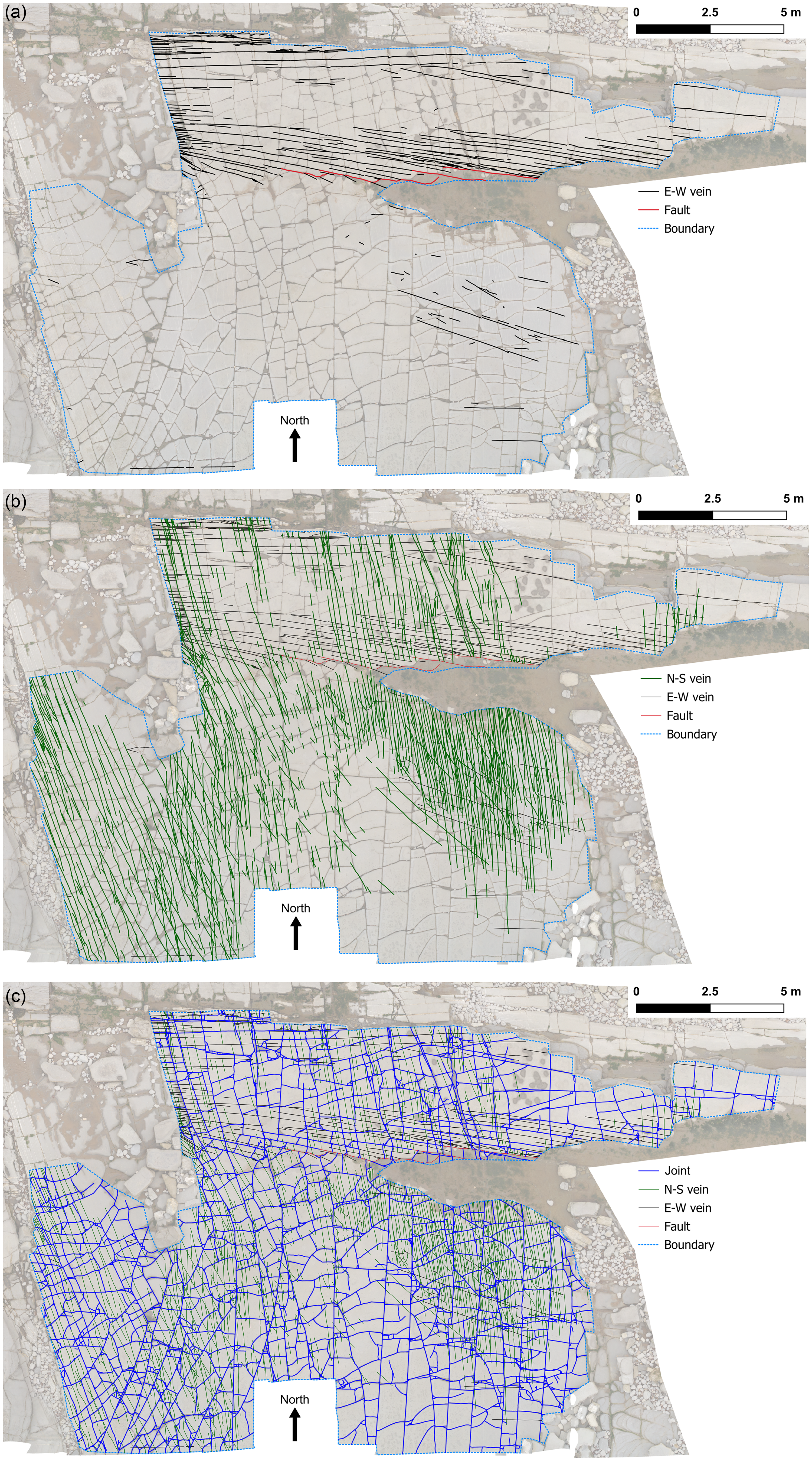
Distributions. Both vein sets appear to show spatial relationships to faults. Set A are clustered around the ∼ E-W-striking faults, with most of the veins of this set occurring in the north of the mapped area (Fig. 6a). Set B is more widely distributed in the mapped area (Fig. 6b) but appears to be concentrated along-strike from faults of similar trend (Fig. 3).
-
Relationships between veins. Some veins of the same set show en echelon relationships, with some pull-aparts developed in veins of Set B. Veins of Set B cross-cut or show trailing relationships with veins of Set A. Some veins of Set B cross-cut other veins of Set B, with ∼ NNW-SSE-striking veins appearing to cross-cut ∼ N-S-striking veins.
-
Relative ages. Crossing and trailing relationships suggest that Set A pre-dates Set B. Crossing relationship of veins of Set B suggests that it may be possible to further divide veins of this orientation on the basis of orientation and relative ages.
Orientation data for the fractures at Lilstock. (a) Rose diagram, weighted to length and area proportional, for the veins (n = 4763). (b) Graph of vein strike vs percentage cumulative branch length for the veins. The straight dashed line, from (0,0) to (180,100), represents a uniform orientation distribution, with deviation of the data from this line providing a useful and unbiased indication of the departure from uniformity (Sanderson & Peacock, Reference Sanderson and Peacock2020). Maximum deviation (D+) = 0.05; minimum deviation (D-) = - 55.09, V = 55.14. The sum V = |D+| + |D-| is independent of the choice of origin, with V = 0 representing a perfectly uniform distribution, and V = 1 representing a parallel alignment of lines (Sanderson & Peacock, Reference Sanderson and Peacock2020). The data indicate a dominant strike of veins at ∼ 145° to 185° (Set B), with a secondary strike of ∼ 085° to 115° (Set A). (c) Rose diagram for the joints (n = 5064). (d) Graph of vein strike vs percentage cumulative frequency for the veins. D+ = 9.1, D- = - 9.5, V = 18.6, V* = 13.26. The data indicate a wider range of strikes than shown by the veins, with a dominant orientation of ∼ 070° to 110°. (e) Rose diagram for the veins and the joints (n = 9827). (d) Graph of vein and joint strike vs percentage cumulative frequency for the veins. D+ = 2.34, D- = - 34.11, V = 36.45, V* = 44.22. The data show intermediate behaviour between the vein and the joint data.

Maps of the different fracture sets at Lilstock. (a) Vein set A strikes approximately E-W and is clustered around a fault zone with an approximate E-W strike. (b) Vein set B strikes approximately N-S to NW-SE and are clustered around faults that strike approximately NNW-SSE. Veins of set B cross-cut or trail through veins of set A. (c) A network of joints is superposed on the pre-existing veins. Some joints cross-cut the veins, while other follow (reactivate) the veins.

5.b. Joint networks
The joints show the following characteristics:
-
Orientations. The joints dip at ∼90° to bedding and their strikes are shown in Fig. 5c, d. Two orientations of joint appear to dominate, these being ∼ N-S and ∼ E-W. The joints that follow veins have, however, the same orientations as vein sets A and B. The sets have a much less clearly defined preferred orientation than the veins, with only ∼80% of the data within broad orientation ranges that occupy ∼70% of the total range. Many of the joints curve, creating problems for subdividing the joints into sets based purely on their orientation (e.g., Engelder & Delteil, Reference Engelder, Delteil, Cosgrove and Engelder2004). For simplicity, we consider the entire joint network to be simply one set, based only on fracture type.
-
Apertures. The joints generally show sub-millimetre apertures. Some wider joints occur, and this probably is caused by weathering and erosion.
-
Trace lengths. The maximum trace length measured for the joints is at least 8.98 m, with this longest joint extending to the edge of the mapping area. The mean length is ∼0.53 m (n = 1881). The joints show a mean trace length per unit area of ∼4.4 m−1.
-
Geometric indicators of kinematics. Joints tend to show opening-mode displacement (e.g., Pollard & Aydin, Reference Pollard and Aydin1988), but curvature along many of the joints may suggest a component of shear along portions of such joints.
-
Distributions. The joints appear to be fairly evenly distributed across the mapped area, with some appearing to curve into fault zones (Fig. 6c). Such behaviours for joints in the Liassic rocks of the Bristol Channel Basin are described by Rawnsley et al. (Reference Rawnsley, Rives, Petit, Hencher and Lumsden1992, Reference Rawnsley, Peacock, Rives and Petit1998) and Bourne and Willemse (Reference Bourne and Willemse2001). The veins appear to be clustered around faults, so the joints that follow veins are also spatially related to faults.
-
Relationships with veins. The joints either cross or follow both sets of veins. The joints that follow the veins do not seem to extend to and beyond the tips of those veins, suggesting that vein aperture is important in controlling whether or not a vein will be reactivated as a joint.
-
Relationships between joints. Pairs of joints in the Liassic rocks of the Somerset coast typically show abutting relationships (e.g., Rawnsley et al., Reference Rawnsley, Peacock, Rives and Petit1998; Peacock et al., Reference Peacock, Sanderson and Rotevatn2018). Some crossing relationships occur where one or both joints follow veins.
-
Relative ages. The joints cross-cut or follow vein sets A and B, so post-date the veins. Abutting relationships between joints would enable relative ages of different joints (or joint sets) to be determined (e.g., Peacock et al., Reference Peacock, Sanderson and Rotevatn2018). Hancock and Engelder (Reference Hancock and Engelder1989) suggest that many joints in northwestern Europe were created by exhumation in a regional stress field in which maximum horizontal compressive stress was orientated ∼ NW-SE.
5.c. Veins and joints combined
Orientation data for the combined populations of veins and joints (Fig. 5e, f) show intermediate behaviour between the orientations of the veins and of the joints independently. Approximately 57.7% of the fracture lengths (veins and joints combined) fall in the strike range of 145°–185°, while approximately 28% of the fracture lengths fall in the strike range of 060°–105°.
6. Topologies of superposed fracture networks at Lilstock
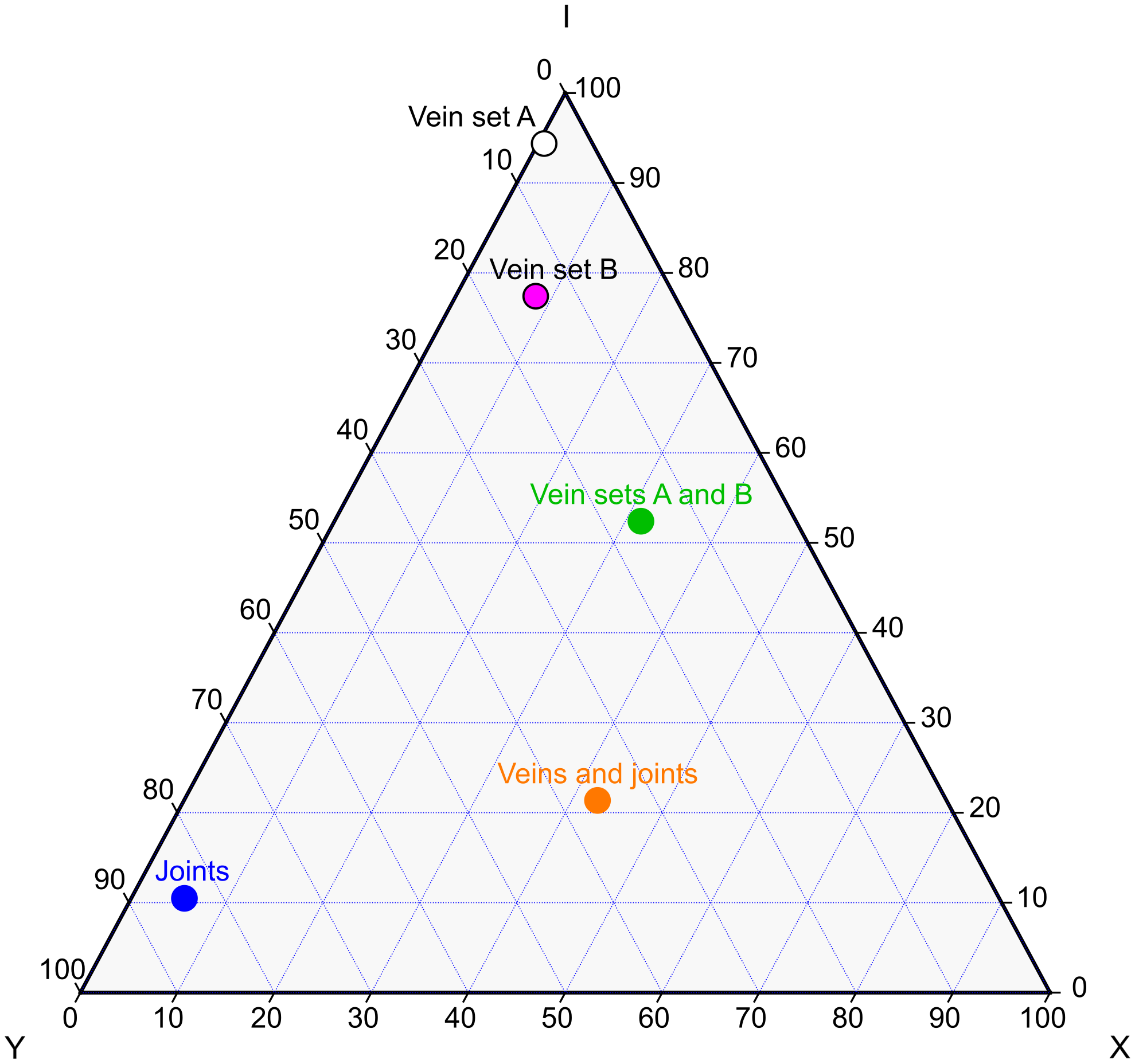
Any network in two dimensions, such as fracture traces, can be represented by a system of nodes and branches (Sanderson & Nixon, Reference Sanderson and Nixon2015). The branches represent the fracture traces and the nodes record information about the types and distributions of intersections between the fractures. Topology emphasizes the relationships between two or more individual structures, such as crossing and abutting relationships of fractures (e.g., Sanderson & Nixon, Reference Sanderson and Nixon2015; Peacock et al., Reference Peacock, Nixon, Rotevatn, Sanderson and Zuluaga2017, Reference Peacock, Sanderson and Rotevatn2018). Network topology is useful for characterizing many aspects of fracture networks (e.g., Sanderson & Nixon, Reference Sanderson and Nixon2015; Duffy et al., Reference Duffy, Bell, Jackson, Gawthorpe and Whipp2015; Procter & Sanderson Reference Procter and Sanderson2018), including establishing the relative age of different structures. It is also useful for understanding the connectivity of fractures within a network (e.g., Berkowitz et al., Reference Berkowitz, Bour, Davy and Odling2000; Manzocchi, Reference Manzocchi2002; Sanderson & Nixon, Reference Sanderson and Nixon2018). Here, we use the node types shown by the different components of the fracture network at Lilstock to show how these differentiate different forms of superposition.
6.a. Vein network
The vein network consists of two sets. Veins in Set A (the older set) are commonly isolated or show en echelon relationships. Set A is dominated by I-nodes (Table 2a, Figs. 6a, 7), which form 92.3% of the nodes. They also have a strong spatial clustering around the faulted margin of the exposed bedding plane.
Node types for the superposed fracture network at Lilstock. (a) Numbers (and percentages) of node types for the components. % C = the percentages of connected nodes (i.e., percentage of V-, Y- and X-nodes). (b) Numbers (and percentages) of connected node types at interactions between different components

Ternary plot of I-, Y- and X-nodes for the veins, the joints and both the veins and joints combined. The vein network is dominated by I-nodes, with more X-nodes than Y-nodes. The joint network is dominated by Y-nodes. The veins and joints combined are dominated by Y- and X-nodes.

Veins in Set B (the younger set of veins) appear to form swarms, with en echelon patterns being less common (Fig. 6b). The Vein B network is still dominated by I-nodes (77.4%), but with significantly more Y- and X-nodes (Table 2). X-nodes are created by cross-cutting relationships between veins in Set B (∼ NNW-SSE striking veins appear to cross-cut ∼ N-S striking veins).
Set B is superposed on Set A creating a higher proportion of X-nodes because the two sets cross (Table 2a, all veins). The two sets of veins combined still shows a majority of I-nodes (52.4%), with 31.5% of the nodes being X-nodes (Table 2a, Fig. 7) at which Set B is seen to cut Set A.
Both Set A and Set B veins develop in damage zones related to two different generations of faults, and this spatial clustering results in limited connectivity across the exposure, with a high proportions of I-nodes. Where superposition occurs, Set A veins are generally overprinted by Set B, producing almost four times as many X-nodes as Y-nodes.
6.b. Joint networks
The joint network is dominated by Y-nodes, these forming 84.6% of the nodes and 94% of the connected nodes (Table 2a, Fig. 7). Prabhakaran et al. (Reference Prabhakaran, Urai, Bertotti, Weismüller and Smeulders2021) report that Y-nodes form 70 to 80% of the nodes in Liassic limestones ∼2.3 km to the east at Lilstock. I-nodes are rare (10.3%; Table 2a), with the joints being highly connected in the network. Six V-nodes were identified, but these are not included in the analysis.
A key feature that distinguished the topology of the joint network is the dominance of Y-nodes, indicating that joints nucleate and/or terminate against one another, which is often termed abutment. This strong interaction contrasts with the cross-cutting and overprinting seen within the vein network. We will examine the interactions between the vein and joint network in the next section.
6.c. Combined network of veins and joints
Combining data for all of the veins and the joints produce a superposed network, with orientations intermediate between the veins and the joints (Fig. 5). At the resolution mapped, the total superposed network has a fracture intensity of just over 10 m−1, with the joints forming 42.4% of this (Table 1). The topology of the combined network (Fractures in Table 2a) is different from either the veins or the joints and cannot be predicted simply from the weighted average of the two networks. The superposed network contains a significantly higher proportion of X-nodes (42.4%) (Table 2a, Fig. 7). We can use the node counts to test hypotheses about the character of the interaction between the two networks.
The data for the connected nodes (Y- and X-nodes) in the vein and joint networks are extracted from Table 2a and combined with data on the number of connected nodes for Set A and Set B intersections and for those between the joints and veins (Table 2b). The proportions of X- and Y-nodes vary between the different types of intersections. Y-nodes dominate (94.5%) for joint:joint intersections, whereas X-nodes dominate (82.1%) for joint:vein intersections. The vein:vein intersections are also dominated by X-nodes but to a somewhat lesser extent (66.1% for all intersections and 78.8% for Set A:B intersections). Table 2a is a simple contingency table with almost zero probability of a random distribution of node types. These data strongly support the idea that vein Set A is overprinted by Set B, but interaction of the joints and veins is more complex. The joints both cross-cut the veins (high % of X-nodes) but also run along (and reactivate) the veins, suggesting both overprinting and utilization of the pre-existing network. The joints dominantly abut other joints, either initiating or terminating at pre-existing joints producing mainly Y-nodes.
7. Discussion
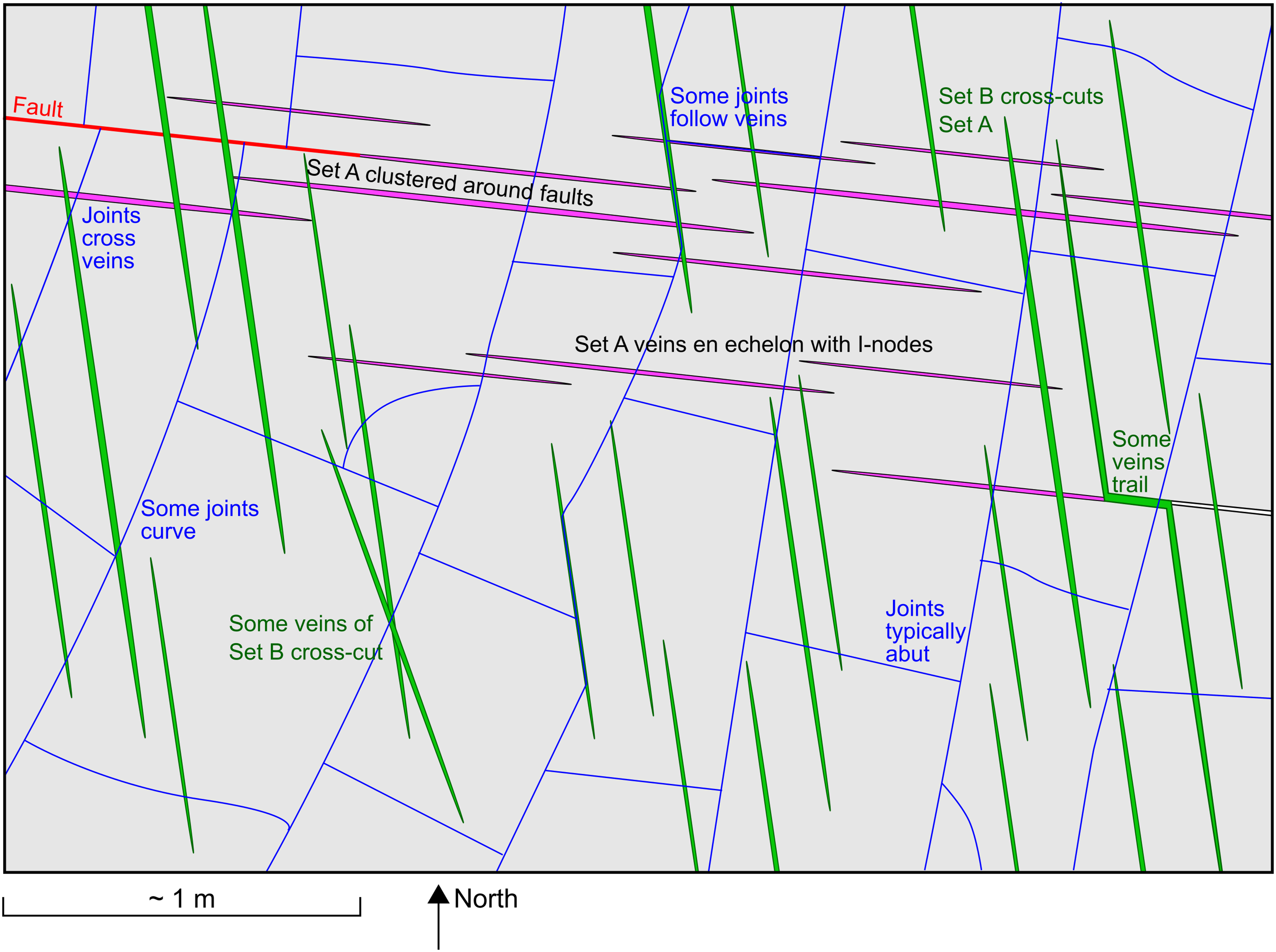
A schematic model for the development of the vein and joint network at Lilstock is shown in Fig. 8. Here, we discuss aspects of the analysis and development of this and other superposed fracture networks.
Schematic model for the superposition of the fracture network at Lilstock. Vein set A is clustered around a fault, with these veins typically being en echelon and forming I-nodes. Vein set B crosses vein set B to form X-nodes, although some trail through veins of Set A. The joints form a later network that cut across or follow veins of sets A and B. Later joints typically abut earlier joints.

7.a. Evolution
The analysis presented here enables the following evolution of the fracture network to be determined. Note that connectivity refers to the degree to which fractures are connected within a network, which depends on the size, frequency, orientation, spatial correlation, scaling and topology (Berkowitz et al., Reference Berkowitz, Bour, Davy and Odling2000; Manzocchi, Reference Manzocchi2002). Three main stages can be identified (Figs. 6, 8):
-
Stage 1: development of vein Set A, in the damage zones of ∼ E-W-striking normal or oblique-slip faults (Fig. 6a). At this stage, the veins are mostly localized adjacent to the faults that bound the area, with little connectivity across the exposed bedding plane.
-
Stage 2: development of vein Set B, in the damage zones of ∼ NW-SE-striking strike-slip faults (Fig. 6b). Some of veins in Set B trail through veins in Set A, while others cross to form X-nodes. At this stage, there was limited connectivity between the Set B veins, but the total vein network is weakly connected across the exposed area.
-
Stage 3: development of the joint network (Fig. 6c). The joints reactivate (follow), trail through or cross-cut the earlier veins. The joint network itself is well connected, mainly through Y-nodes, with few I-nodes. The joint network overprints and reactivates the vein network to produce a superposed vein–joint network that is well-connected network.
The sequential evolution of network connectivity has been documented by Park et al. (Reference Park, Kim, Ryoo and Sanderson2010). Determining this evolution requires both identification of the types of fracture involved and examination of their relationships (reactivation, trailing, crossing, etc.).
7.b. Overprinting and reactivation
The superposition of two or more fracture networks can occur in different ways. The N-S veins largely overprint the E-W veins, producing cross-cutting intersections (high proportion of X-nodes in Table 2), with a limited amount of reactivation, as indicated by occasional trailing. The joint network shows both overprinting, abutting (Y-nodes) and much re-utilization of the earlier formed veins (joints along veins), with abundant termination and trailing of joints at veins and particularly at earlier formed joints.
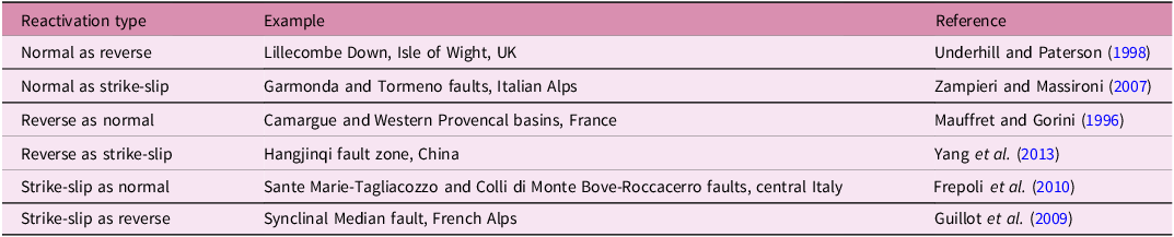
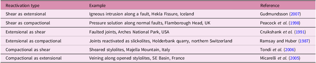
Fracture reactivation is a common form of superposition. Faults are commonly reactivated with a different sense of displacement, with examples given in Table 3. This reactivation can be a component of fracture network superposition. For example, Kelly et al. (Reference Kelly, Peacock, Sanderson and McGurk1999) show that reverse-reactivation of E-W-striking normal faults in the Liassic rocks at East Quantoxhead (∼5 km WSW of the study area at Lilstock) was accompanied by the development of a network of conjugate strike-slip faults. Fracture network superposition can also involve fractures being reactivated as other types of fractures, such as an extension fracture (e.g., a vein or a joint) being reactivated as a contractional structure (e.g., a stylolite). Examples of such reactivation are given in Table 4.
Examples of different types of fault reactivation

Examples of different types of fracture reactivation

7.c. Implications for analysing and understanding fracture networks
Just as understanding superposed folding helps unravel the deformation history of a region (e.g., Ray, Reference Ray1974; Ramsay & Huber, Reference Ramsay and Huber1987), understanding superposition in fracture networks helps determine the evolution of that network. Rather than analysing the final fracture network as a single entity (e.g., Zhu et al., Reference Zhu, He, Santoso, Lei, Patzek and Wang2022), it is necessary to distinguish the different fracture types present and determine the sequence of development of the components of the network (e.g., Katternhorn et al., Reference Kattenhorn, Aydin and Pollard2000; Gillespie et al., Reference Gillespie, Walsh, Watterson, Bonson and Manzocchi2001), if the geometric and topological development of the network is to be understood. This involves using geometric and topological characteristics to define different classes or ages of fracture that are appropriate for the study (e.g., Peacock & Sanderson, Reference Peacock and Sanderson2018; Andrews et al., Reference Andrews, Shipton, Lord and McKay2020). Such an approach helps deduce how fractures have been controlled by the interplay between palaeostress fields and earlier structures and would lead to better understanding of the kinematic, tectonic and fluid flow history. Simply adding all fractures together in a network would be analogous to not distinguishing between paths, roads, canals, railways and aeroplane flight paths, and lumping them all together to analyse a transport network.
7.d. Other network components and examples
While we have focused on a fracture network created by the superposition of two sets of veins and a joint network, the analysis can be expanded to include other structures in the network. For example, some of the stepping veins of Set B are linked by stylolites or slickolites, with some forming pull-aparts (e.g., Willemse et al., Reference Willemse, Peacock and Aydin1997). At a larger scale, the two vein sets appear to be damage related to a network of superposed faults (Fig. 3). Superposed fault networks can show abutting (e.g., Nixon et al., Reference Nixon, Sanderson, Dee, Bull, Humphreys and Swanson2014, Fig. 11), crossing (e.g., Dart et al., Reference Dart, McClay, Hollings, Buchanan and Buchanan1995; Gonzalo-Guerra et al., Reference Gonzalo-Guerra, Heredia, Farias, García-Sansegundo, Martín-González, Butler, Torvela and Williams2023), reactivating (Table 3) or trailing (Nixon et al., Reference Nixon, Sanderson, Dee, Bull, Humphreys and Swanson2014, Fig. 15) relationships.
8. Conclusions
Superposed fracture networks result from the successive development of different ages (and commonly different types) of fractures. Successive sets of fractures may either overprint (cross-cut), follow (reactivate) or arrest at (abut) the earlier ones. In the example of veins and joints on a Liassic limestone bedding plane at Lilstock, UK, the network comprises (1) early formed E-W veins, (2) later N-S veins and (3) a later system of joints. The later components of a superposed fracture network can both overprint and re-utilize (reactivate) earlier fractures. For example, the N-S veins at Lilstock cross-cut and trail into E-W veins, and the joints abut, cross-cut and reactivate both the vein sets.
The different components of a superposed fracture network can have different topologies. The first set of veins at Lilstock is dominated by I-nodes, with linkage of the straight, sub-parallel veins being limited. The second set of veins is still dominated by I-nodes, but locally cross-cut Set A, producing more X-nodes. The joints cross-cut both sets of veins, producing X-nodes. This indicates overprinting of the vein network by joints, but that some utilizing earlier veins as they develop. Joint:joint intersections are dominantly Y-nodes, indicating strong mechanical interaction during joint development.
When interpreting a superposed fracture network, it is important to separate out the components, based on both the type of fracture and their age relationships. Although we have focused on veins and joints, this type of analysis is applicable to other types of superposed fracture networks, including faults.
Acknowledgements
M. Magán was supported by a Severo Ochoa grant and project AYUD/2021/51293 funded by the Government of Asturias and by Research project PID2021-126357NB-100 funded by the Spanish Ministry of Science and Innovation. We thank Billy Andrews, Tom Blenkinsop and an anonymous reviewer for their useful comments.
Competing interests
The authors declare none.

 Open access