





1. Introduction and background
Changes in ice sheet mass directly impacts sea-level change, so Greenland and Antarctica’s net mass balance have been the focus of a great deal of recent scientific research (Rignot and others, Reference Rignot, Mouginot, Scheuchl, van den Broeke, van Wessem and Morlighem2019; Mankoff and others, Reference Mankoff2021; Fox-Kemper and others, Reference Fox-Kemper, Masson-Delmotte, Zhai, Pirani, Connors, Péan, Berger, Caud, Chen, Goldfarb, Gomis, Huang, Leitzell, Lonnoy, Matthews, Maycock, Waterfield, Yelekçi, Yu and Zhou2023; Otosaka and others, Reference Otosaka2023; and many others). The mass loss from the grounded portion of the Greenlandic and Antarctic ice sheets contributes to sea level rise (SLR), and can be captured by a single value or time series per ice sheet. Reporting a single value or time series derived from multiple years of data is beneficial because it simplifies interpretation and comparison. However, ice sheets are complex systems, and while their contribution to sea level rise is important, focusing on their SLR contribution alone provides minimal understanding of the processes at play, and how they change. As one example, an ice sheet that increases output via discharge but has that offset by an equal increase in inputs (e.g., snowfall) would report a neutral mass balance and no change in contribution to SLR, but has entered a different state when viewing constituent terms. Few studies consider all mass transport pathways and their relative magnitudes and uncertainties – this is typically limited to review papers, which may not focus on quantitative assessment of each process.
Studies that assess mass balance typically use one or a combination of three methods.
The gravimetric mass balance (GMB) method directly measures changes in the gravitational field generated by the ice sheets. It is observation-based and excels at measuring the grounded ice contribution to sea level rise, but cannot observe changes in floating ice as these do not cause changes in the gravitational field, nor distinguish processes that contribute to changes of the grounded ice. Spatial resolution is  $\sim$100 km and temporal resolution is monthly (e.g.,
Groh and others, Reference Groh2019; Döhne and others, Reference Döhne, Horwath, Groh and Buchta2023).
$\sim$100 km and temporal resolution is monthly (e.g.,
Groh and others, Reference Groh2019; Döhne and others, Reference Döhne, Horwath, Groh and Buchta2023).
The volumetric method estimates the total volume and change in volume of the ice sheets from altimetry. This method is also observation-based, has spatial resolution of  $\sim$1000 m and temporal resolution is monthly (cf. Simonsen and others, Reference Simonsen, Barletta, Colgan and Sørensen2021; Khan and others, Reference Khan2022). It can be used over floating ice, and this is the primary method for observing ice shelf thinning from which ice shelf basal melt is inferred (e.g.,
Greene and others, Reference Greene, Gardner, Schlegel and Fraser2022; Davison and others, Reference Davison2023). However, the volumetric method cannot be used to distinguish between surface and grounded basal processes and only reports total thinning (cf. Karlsson and others, Reference Karlsson2021).
$\sim$1000 m and temporal resolution is monthly (cf. Simonsen and others, Reference Simonsen, Barletta, Colgan and Sørensen2021; Khan and others, Reference Khan2022). It can be used over floating ice, and this is the primary method for observing ice shelf thinning from which ice shelf basal melt is inferred (e.g.,
Greene and others, Reference Greene, Gardner, Schlegel and Fraser2022; Davison and others, Reference Davison2023). However, the volumetric method cannot be used to distinguish between surface and grounded basal processes and only reports total thinning (cf. Karlsson and others, Reference Karlsson2021).
Finally, the input–output (IO) method is a hybrid of regional climate models (RCM) and observations (flow velocity, ice thickness; e.g., Gardner and others, Reference Gardner2018; Mouginot and others, Reference Mouginot2019; Rignot and others, Reference Rignot, Mouginot, Scheuchl, van den Broeke, van Wessem and Morlighem2019; Mankoff and others, Reference Mankoff2021). This method estimates inputs (e.g., snowfall) and outputs (e.g., surface melt and iceberg calving), and is typically reported at the low spatial resolution of individual glacier basins. Temporal resolution is  $\sim$10 days or whenever a new velocity map is generated, but given the stability of the ice flow compared to the daily variability the surface mass balance (SMB), the IO method can provide some estimate of daily mass balance (Mankoff and others, Reference Mankoff2021). The IO method is the only one that captures all of the processes contributing to changes of grounded ice and provides gross values and constituent terms.
Here we use a combination of the IO method over grounded ice, the altimetry method over ice shelves, and other individual remote sensing estimates of ice shelf and glacier front advance and retreat. We provide results both in tabular form, and using Sankey diagrams that provide a visual method to compare magnitude of all processes within and between ice sheets, and flows representing relations between processes.
1.1. Introduction to Sankey diagrams
Sankey diagrams are graphical representations of flow or movement of any property (e.g., mass, energy, money, etc.). An early and famous use was Charles Minard’s Map of Napoleon’s Russian Campaign of 1812 (cf. Kraak, Reference Kraak2021) that combines the magnitude of active soldiers overlaid on a geographical map. The method was later refined, popularized, and eventually named after Captain Matthew Henry Phineas Riall Sankey who used it to show, among other things, the energy efficiency of a steam engine.
A similar display to the diagrams presented here, by Cogley and others (Reference Cogley2011, Fig. 2), shows glacial processes overlaid on a glacier schematic. We build on that work by adding magnitude of processes and making the graphics proportional to magnitudes.
Appendix A has details on the software used to generate these Sankey diagrams.
1.1.1. Interpreting these Sankey diagrams
Sankey diagrams are generally intuitive, but the following section may still be helpful in interpreting the diagrams shown here.
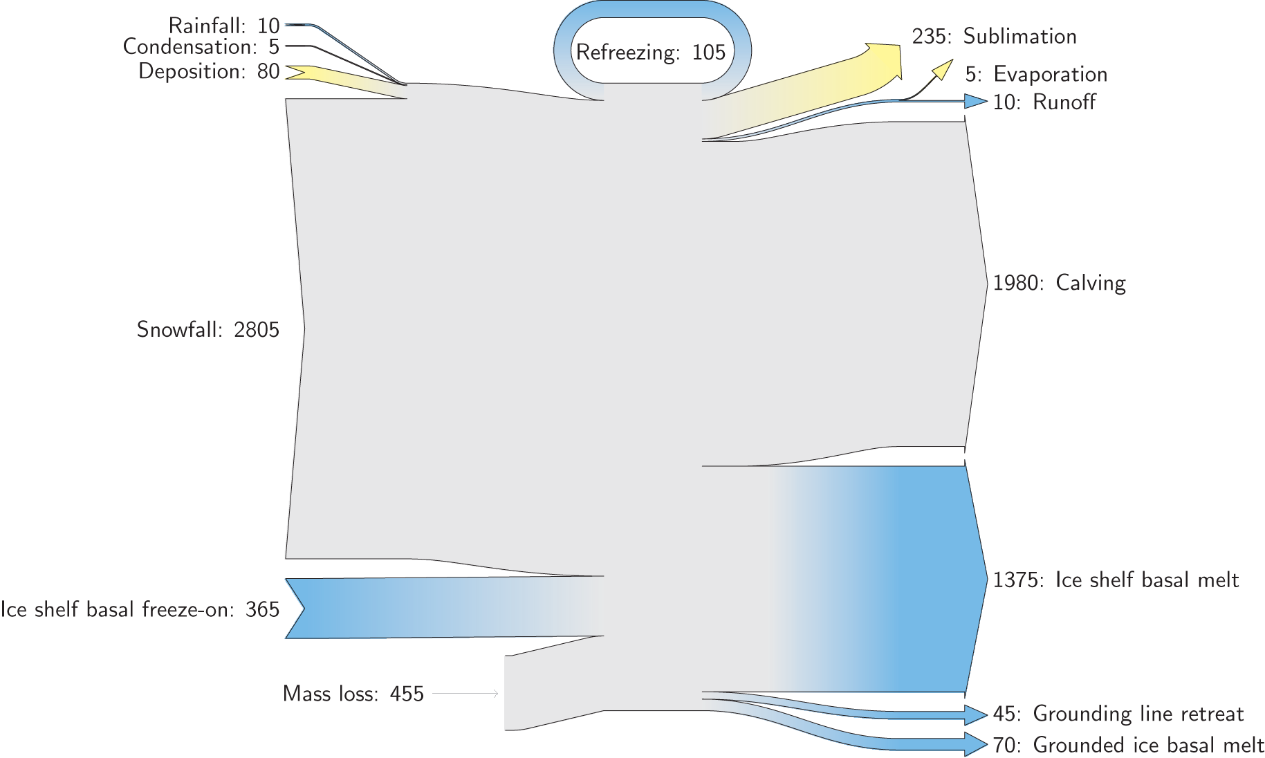
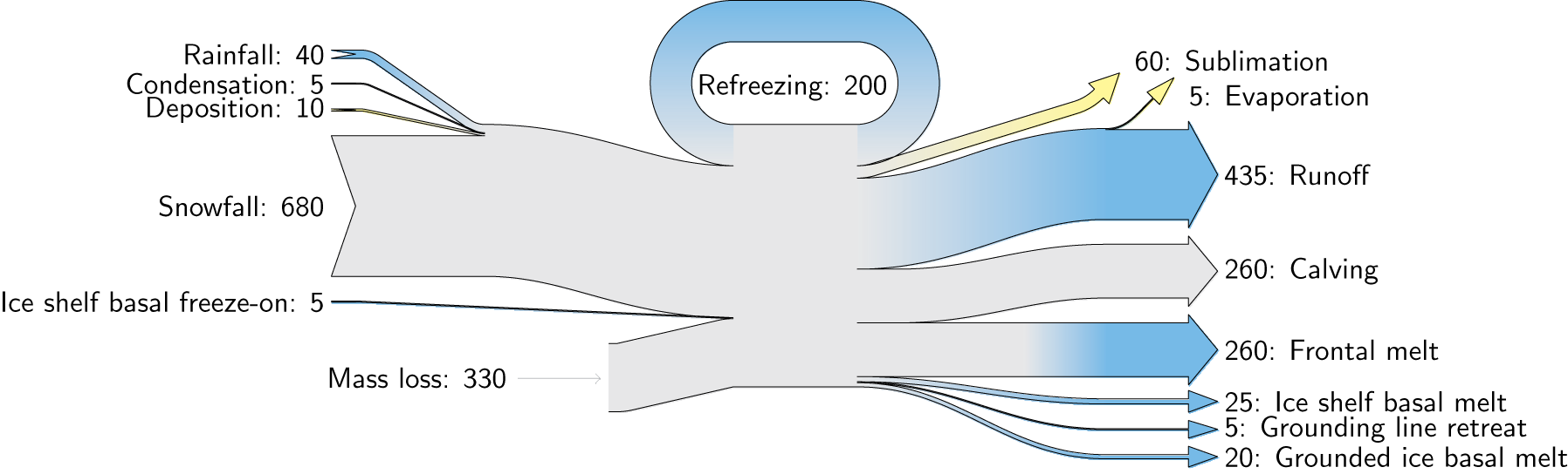
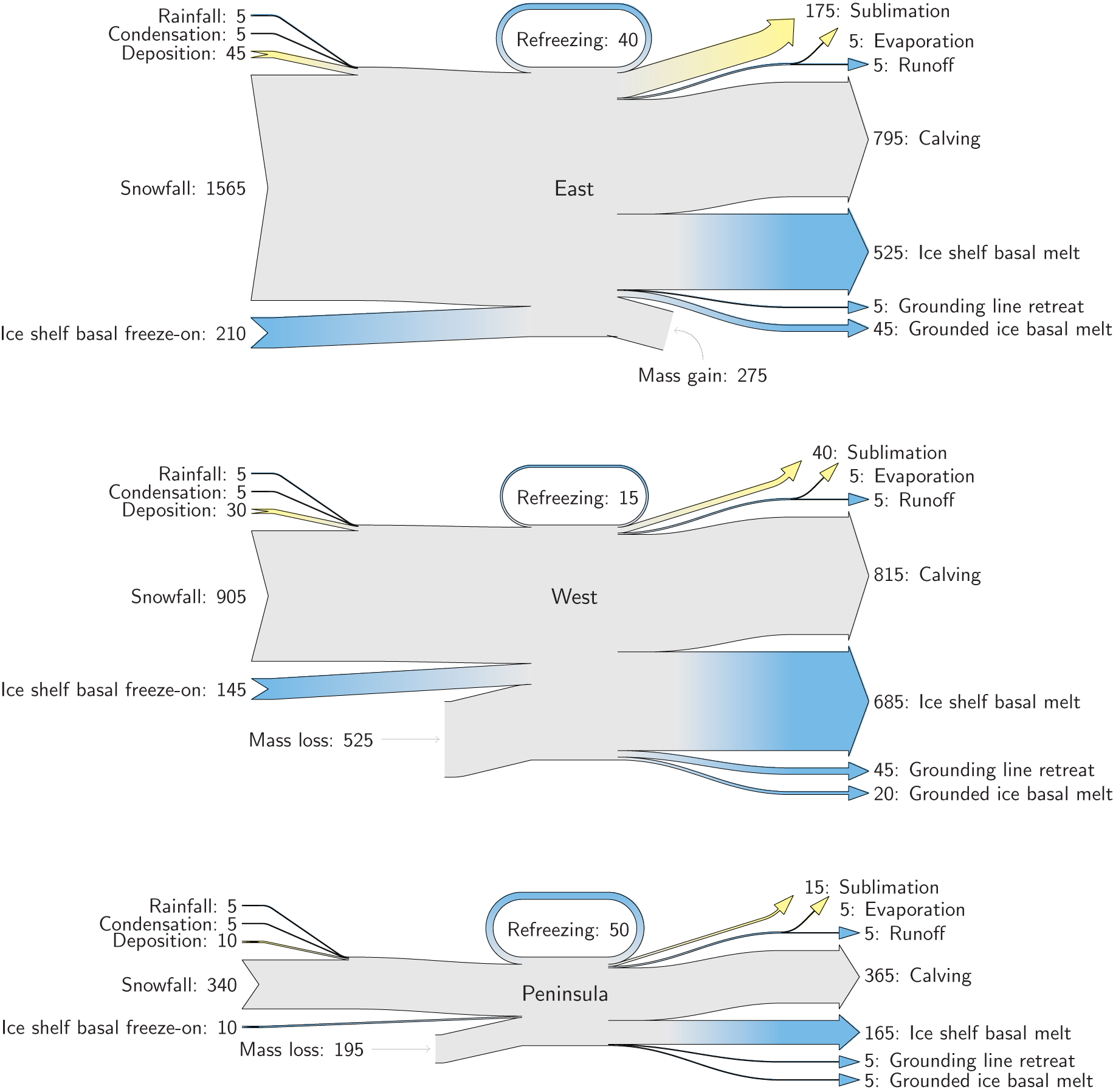
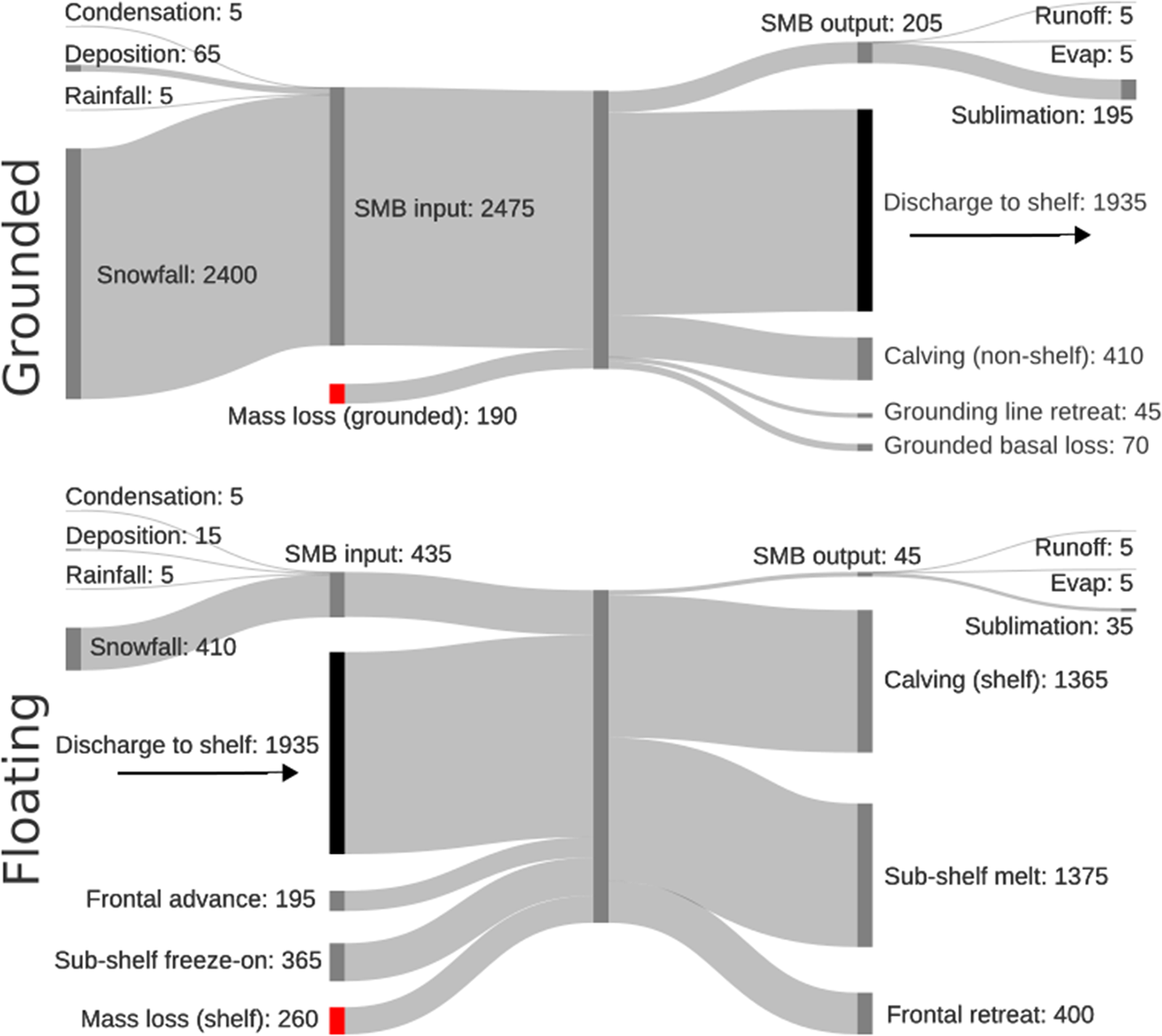
The widths of all lines are all proportional to each other both within and among Figs 1, 2, and 3 but not Fig. 4.
Sankey mass flow diagram for Greenland. Numbers are mass flow rate [Gt yr $^{-1}$]. All widths are proportional within and between images. Gray is solid phase, blue is liquid phase, and yellow is gas phase. Inputs (left, arrow tail) are balanced by outputs (right, arrow head) and come from IO column of Table 1. Because Sankey diagrams balance all inputs and outputs, mass losses require an input to balance the larger outputs.

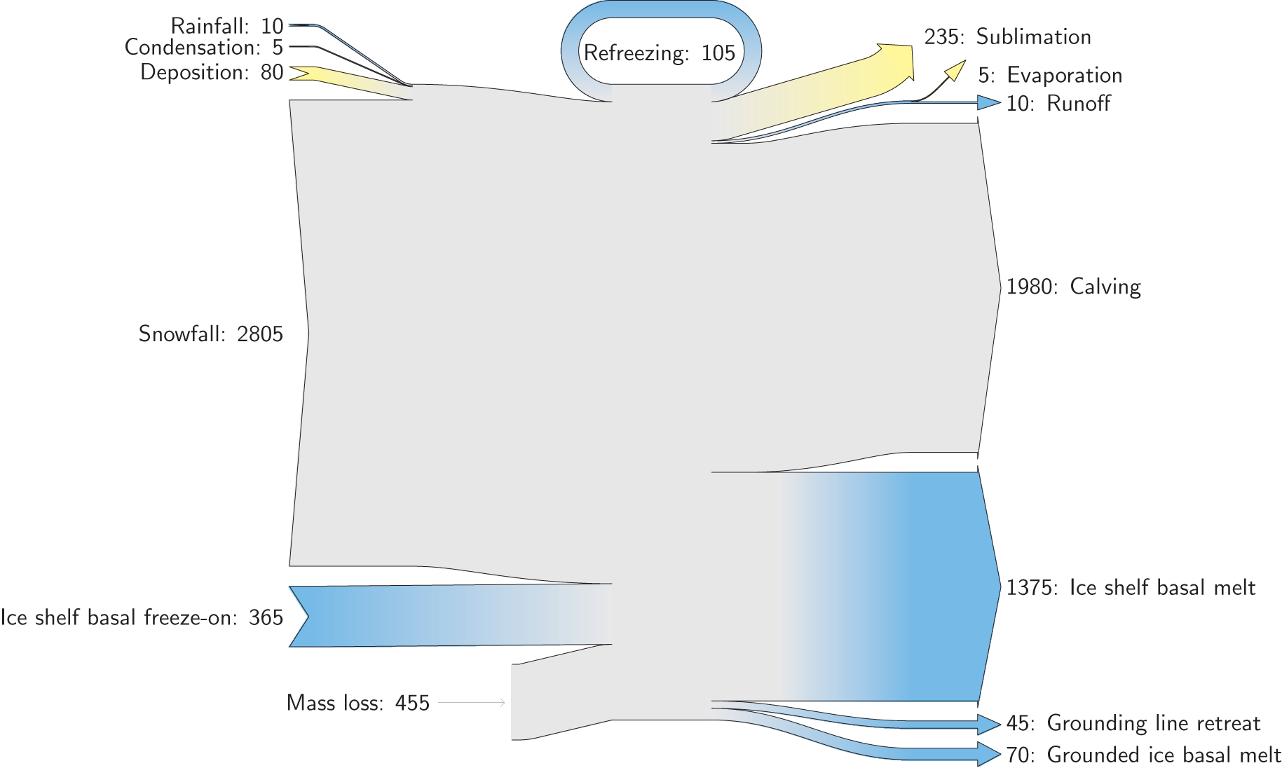
Sankey mass flow diagram for Antarctica. See Figure 1 for legend and details.
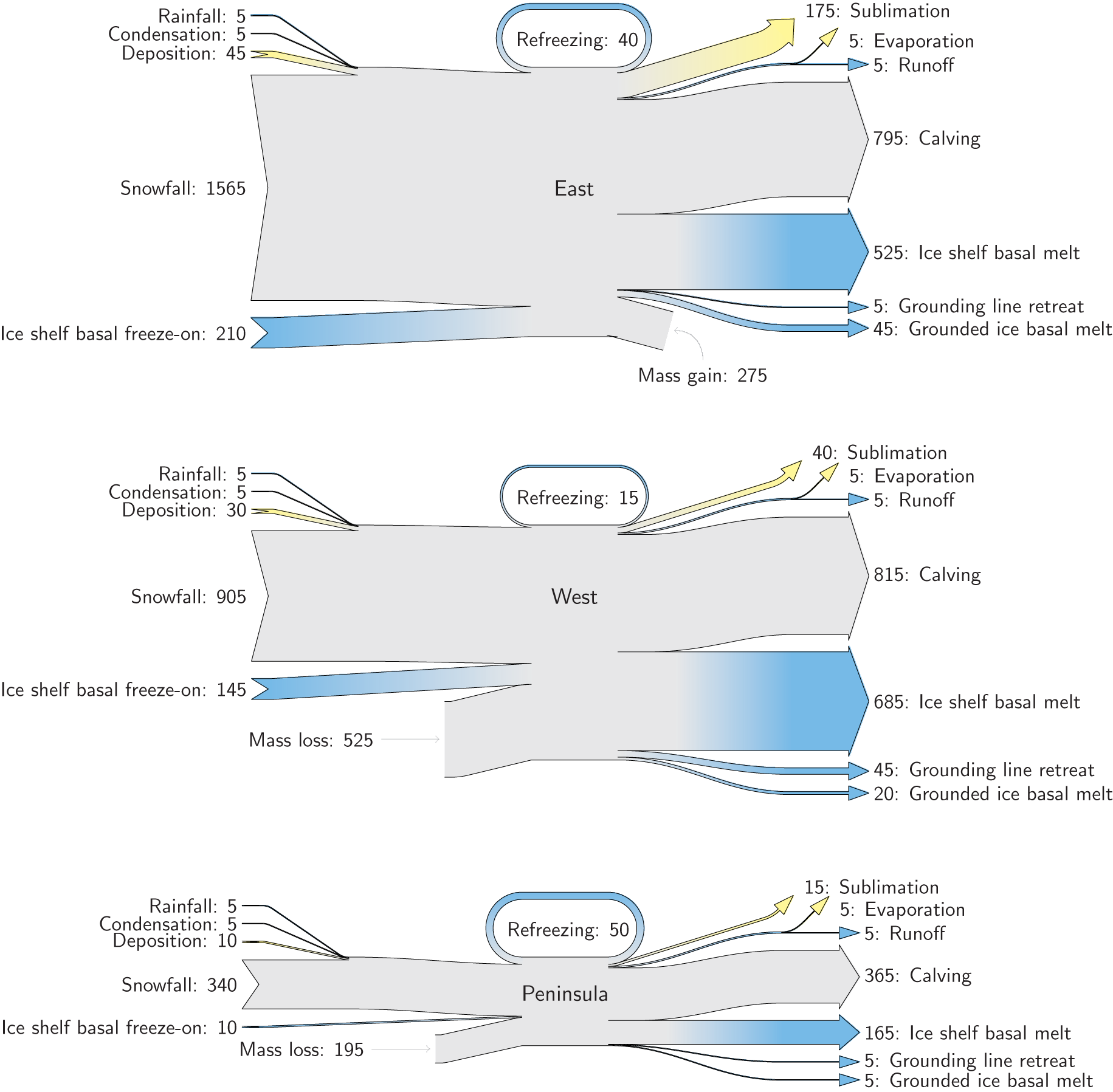
Sankey mass flow diagrams for three Antarctica regions: East, West, and Peninsula. Numbers are mass flow rate [Gt yr $^{-1}$]. All widths are proportional within and between images (and Figs 1 and 2). In East Antarctica mass gain is an output at the bottom that balances the diagram, because without it, there are more flows into the system than out of it.
Sankey mass flow diagrams for Antarctica split by grounded vs. floating ice. Upper and lower figure should be merged at vertical black bar, where mass flow output from grounded ice is mass flow input to ice shelves. Numbers are mass flow rate [Gt yr $^{-1}$]. Unlike other figures, here frontal retreat, frontal advance, and calving are shown gross not net as delivered in the upstream products. This display choice makes it challenging to see, for example, net SMB terms which are readily available in Figs 1, 2, and 3. Even more involved displays with more branches (and possibly crossed paths) could show all relevant terms both in isolation (e.g., by region and process) and in combination.

Sankey diagrams balance all inputs and outputs, which introduces a complication for the use case here due to the mass imbalance. Traditionally, when a Sankey diagram has a loss term, it is an output. For example, all engines have energy inputs greater than outputs, the ratio between the two is a measure of efficiency, and the energy lost between input and output is displayed as an additional output (typically waste heat).
In the Sankey diagrams here with net mass loss (i.e., ice sheet drawdown or retreat), outputs are greater than inputs, so mass loss must then be a balancing input representing drawdown of the historical ice mass or retreat of the ice sheet boundary. In the Sankey diagrams with net mass gain (i.e., build-up or expansion), inputs are larger than outputs, so mass gain is a balancing output representing ice build-up or boundary expansion. These two special terms – mass loss or gain – are shown with truncated arrows in Figures 1 through 3.
Finally, the Sankey diagrams shown here are simplistic representations of mass flow across the three ice sheet boundaries (atmospheric, subglacial, and oceanic). We combine all inputs and outputs, not distinguishing between inputs over grounded ice vs. inputs over ice shelves, or other display options. However, alternate displays are possible, and a more complex display is shown in Fig. 4 which separates inputs and outputs by region (grounded, floating) in Antarctica.
2. Terminology
We use the common terms from Cogley and others (Reference Cogley2011) with a few clarifying points. We refer readers to Figure 2 of Cogley and others (Reference Cogley2011) for a graphical schematic showing mass flow pathways overlaid on a glacier including phases (solid, liquid, gas), and boundaries (atmospheric, subglacial, oceanic).
Our estimates of mass flow include all ice in Greenland and Antarctica, including peripheral glaciers.
We use ‘grounding line’ to refer to the ice/ocean/bed interface underneath ice shelves and floating ice tongues. When there is no ice shelf, we use the term ‘front’ as in ‘calving front’ or ‘frontal advance.’
Sublimation from SMB is often a net term that includes condensation (the process of gas transforming directly to a liquid), deposition (gas to solid), evaporation (liquid to gas), and sublimation (solid to gas). Here, we distinguish between all unique four types of phase transitions. Runoff is meltwater or rain that does not refreeze and instead leaves the ice sheet.
This work does not explicitly report submarine melt, the sum of all melt that occurs underwater, but instead we use and report constituent terms when available. Frontal melt is from vertical faces at the calving edge of Greenlandic glaciers. There are no estimates of frontal melt at the calving edge of Antarctic ice shelves or non-shelf calving regions, but mass flow across this boundary is then included in the calving estimates. Ice shelf basal melt is from horizontal surfaces under ice shelves in Greenland and Antarctica.
We do not use the term ‘basal melt’ because it does not distinguish between grounded or floating ice. Instead we use ‘ice shelf basal melt’ and ‘grounded ice basal melt.’
We generally avoid the term ‘flux’ which by definition is per unit area. Because we do not report results per unit area, we use ‘mass flow rate’ [Gt yr $^{-1}$].
Not all processes are directly observable due to limitations in measurements, nor are they all modeled. We are limited by the data provided in the products that we ingest to this work. We therefore sometimes report process and sometimes product. In many cases products and process are the same (e.g., ‘snowfall’ process and the ‘snowfall’ data product from the RCM). An example where product rather than process is presented is the ‘frontal retreat’ data product which is a combination of the calving and frontal melting processes. An example where processes rather than product is presented is the Greenland ice discharge product which is not shown because discharge is measured a few km upstream of the grounding line. Instead, we show the downstream calving and frontal melt processes.
3. Methods
The full methods (source code) for this manuscript can be found at https://doi.org/10.5281/zenodo.15819650 which archives and assigns a DOI to releases made from the source code repository at https://github.com/mankoff/sankey.
Below we detail the source of each mass flow term. We begin with the outputs as these are generally of broader interest, followed by the inputs. We then describe how net mass loss or gain are computed, and how uncertainty is estimated. Finally, we address other methods such as regional separation, temporal alignment, and rounding.
3.1. Outputs
3.1.1. Sublimation, evaporation, and runoff
We use constituent terms (i.e., gross, not net) of SMB from the Modèle Atmosphérique Régional (MAR) RCM for both Greenland (Fettweis and others, Reference Fettweis2020) and Antarctica (Kittel and others, Reference Kittel2021).
3.1.2. Calving, frontal melt, and ice shelf basal melt
In Greenland, we use ice discharge across flux gates  $\sim$5 km upstream from the grounding lines (Mankoff and others, Reference Mankoff2021). That discharge term at the flux gates is known to overestimate discharge across the downstream grounding line because it neglects SMB losses between the flux gate and grounding line. These losses are estimated at $\sim$17 Gt yr $^{-1}$ by Kochtitzky and others (Reference Kochtitzky2023) who uses flux gates closer to the grounding line than the Mankoff and others (Reference Mankoff, Solgaard, Colgan, Ahlstrøm, Khan and Fausto2020b) flux gates. The elevation of flux gates used by Mankoff and others (Reference Mankoff, Solgaard, Colgan, Ahlstrøm, Khan and Fausto2020b) were typically located tens to hundreds of meters higher (and therefore further from the calving front) than the flux gates used by Kochtitzky and others (Reference Kochtitzky2023). We estimate an average of $\sim$3 Gt yr $^{-1}$ are lost to surface melt while the ice transits this region. When estimating discharge from the perimeter of the ice sheet, we therefore subtract 20 Gt yr $^{-1}$ from the more inland observations by Mankoff and others (Reference Mankoff, Solgaard, Colgan, Ahlstrøm, Khan and Fausto2020b) meaning frontal melt and calving are each reduced by 10 Gt yr $^{-1}$ (see below for discharge split to frontal melt and calving). Peripheral glaciers are not included in the Mankoff and others (Reference Mankoff, Solgaard, Colgan, Ahlstrøm, Khan and Fausto2020b) product, but are added through estimates from Bollen and others (Reference Bollen, Enderlin and Muhlheim2023).
Greenlandic discharge from the flux gates is split into either calving or frontal melt at the calving front, which is the grounding line if no ice shelf is present, or shelf front if an ice shelf is present. This split is highly uncertain and minimally studied, but Rignot and others (Reference Rignot, Koppes and Velicogna2010) estimate that 20–80% of the summer ice-front is directly melted by the ocean for the three glaciers they studied. From this, we split the discharge 50  $\pm$30% between calving and frontal melt.
In Antarctica, calving includes grounded ice that leaves the ice sheet directly into the ocean (not an input to an ice shelf; Rignot and others, Reference Rignot, Mouginot, Scheuchl, van den Broeke, van Wessem and Morlighem2019) and ice shelf calving from Greene and others (Reference Greene, Gardner, Schlegel and Fraser2022). We assume that the Antarctic frontal melt component is zero.
Both Antarctic calving and Greenlandic calving and frontal melt are provided as ‘steady state’ terms in Tables 1 and 2. That is, in Greenland calving and frontal melt balances grounded ice discharge and does not include frontal advance and retreat, which come from a separate product and are presented as their own term in the tables. In Antarctica, non-shelf calving balances non-shelf discharge, and ice shelf calving is based on a fixed calving front. See frontal advance and frontal retreat for the non steady state component. However, the graphics combine the frontal advance and frontal retreat terms. Both calving and frontal melt change by half of frontal retreat minus frontal advance. In Antarctica, calving is increased by frontal retreat minus frontal advance.
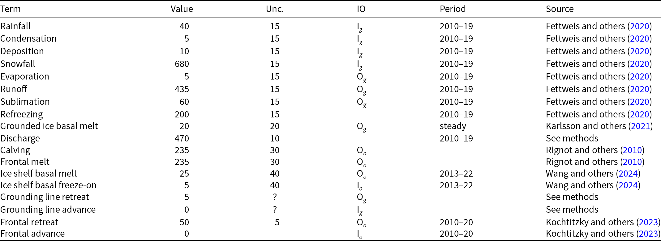
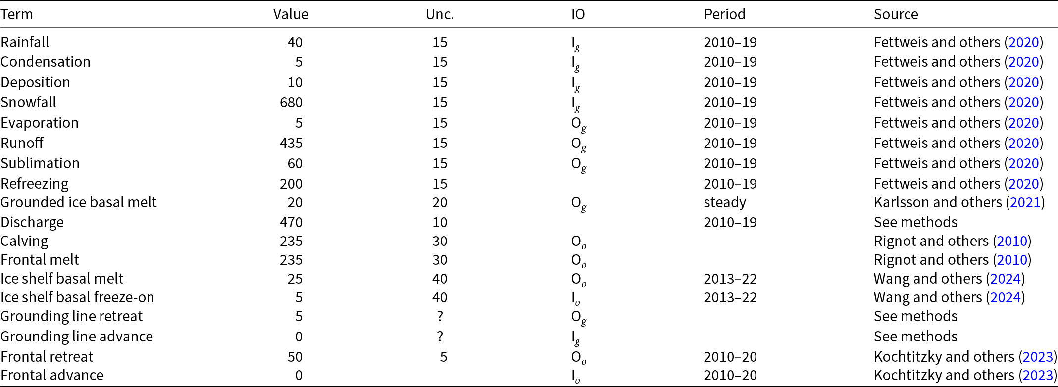
Greenland mass flow terms, values [Gt yr $^{-1}$], uncertainty (Unc.) [%], and metadata. IO encodes input (I) or output (O) to or from grounded ice (subscript g) or ocean (subscript o). The 15% uncertainty reported for the SMB components (top eight rows) is from net SMB, not the individual components. Some terms in the table are combined in the graphics – see Methods.
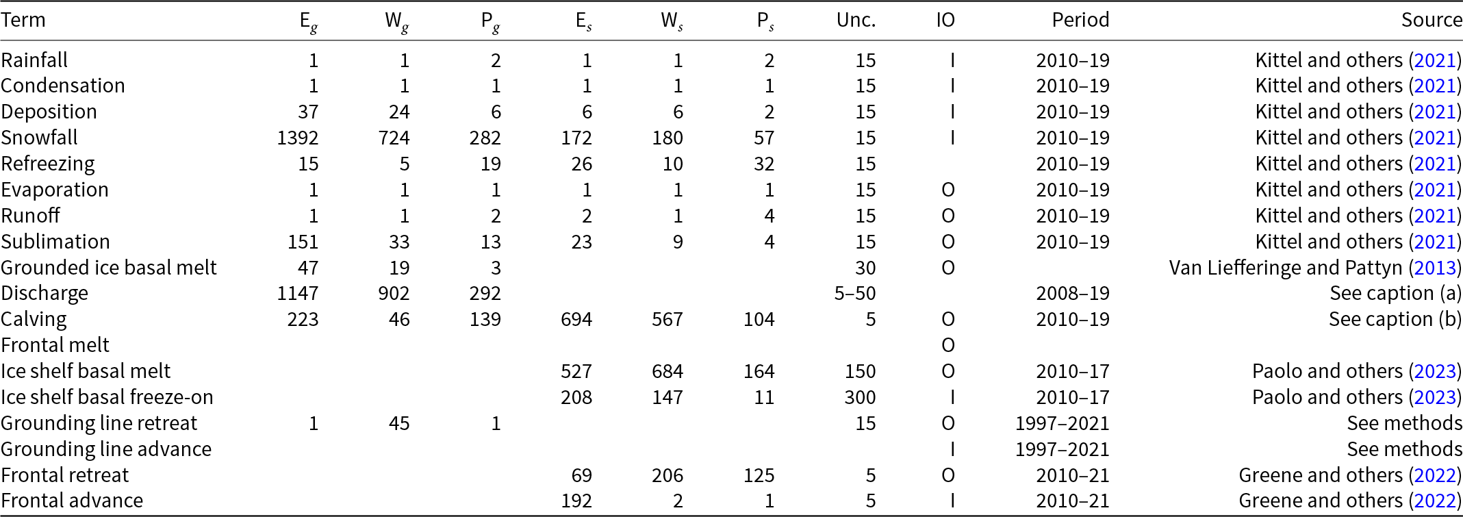
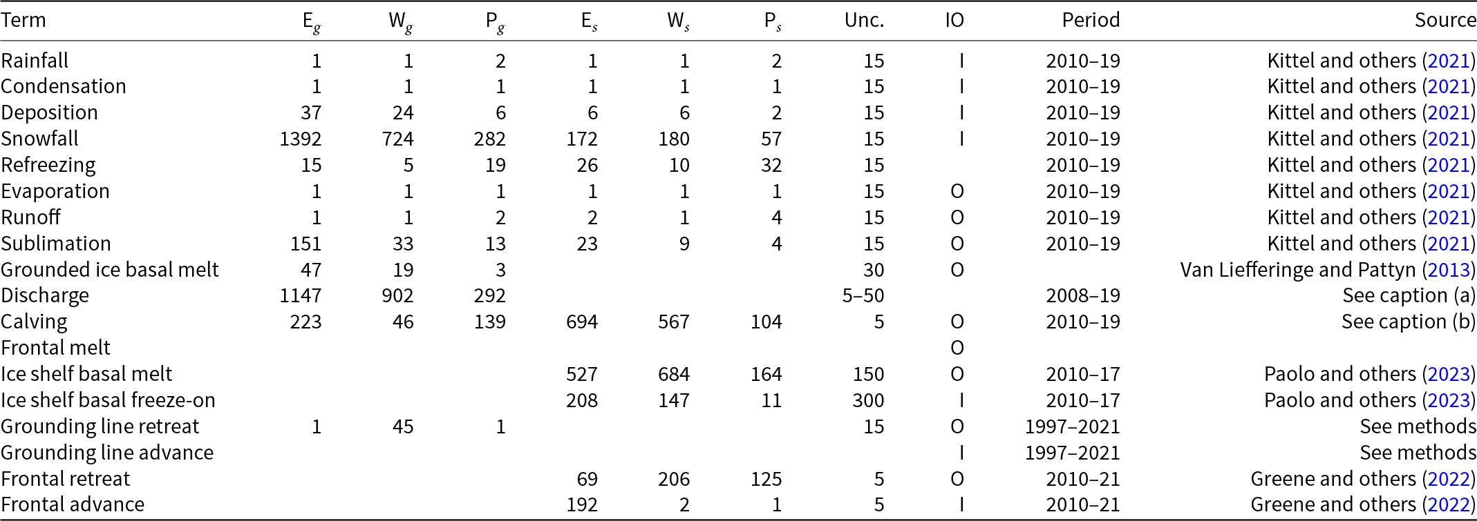
Antarctic mass flow terms. E, W, and P represent East, West, and Peninsula regions respectively. Subscripts g and s represent grounded and shelf components respectively. IO encodes if the Term is an input (I) or an output (O). Values are in units Gt yr $^{-1}$ except Unc. (uncertainty) which is %. Values are rounded to nearest integer except values $ \lt 0.5$ are rounded up to 1. (a) Discharge is grounded ice discharge to ice shelves from Davison and others (Reference Davison2023) plus grounded ice discharge from non-shelf coastal regions and from islands from Rignot and others (Reference Rignot, Mouginot, Scheuchl, van den Broeke, van Wessem and Morlighem2019). (b) Calving is ice shelf terminus calving from Greene and others (Reference Greene, Gardner, Schlegel and Fraser2022) plus grounded ice calving from non-shelf coastal regions and from islands from Rignot and others (Reference Rignot, Mouginot, Scheuchl, van den Broeke, van Wessem and Morlighem2019). The 15% uncertainty reported for the SMB components (top eight rows) is from net SMB, not the individual components. Some terms in the table are combined in the graphics – see Methods.
Ice shelf basal melt in Greenland comes from Wang and others (Reference Wang2024), and in Antarctica comes from Paolo and others (Reference Paolo2023).
3.1.3. Frontal retreat
The frontal retreat products for Greenland (Kochtitzky and others, Reference Kochtitzky2023) and Antarctica (Greene and others, Reference Greene, Gardner, Schlegel and Fraser2022) are one part of the non ‘steady state’ component of calving and frontal melt processes (the other part being frontal advance). Here we report the net products in the tables (frontal retreat) and the gross processes (calving, frontal melt) in the graphics. Net frontal retreat is split between frontal melt and calving processes  $\sim$50/50 in Greenland (Rignot and others, Reference Rignot, Koppes and Velicogna2010) with high uncertainty, and is likely to be primarily calving in Antarctica. Frontal advance is discussed in the Inputs section.
3.1.4. Grounding line retreat
Grounding line retreat by definition here only occurs under ice shelves. If there is no ice shelf, it is frontal retreat.
Numerous papers have documented grounding line migration around both Greenland and Antarctica at different spatial and temporal scales (e.g.,
Rignot and others, Reference Rignot, Mouginot, Morlighem and Scheuchl2014; Konrad and others, Reference Konrad2018; Milillo and others, Reference Milillo2022; Millan and others, Reference Millan2022a; Gadi and others, Reference Gadi, Rignot and Menemenlis2023; Li and others, Reference Li, Dawson, Chuter and Bamber2023; Picton and others, Reference Picton, Stokes, Jamieson, Floricioiu and Krieger2023). However, only one study (Davison and others, Reference Davison2023) provides estimates of grounding line migration in the dimensions needed here, mass or length3 and time (e.g., Gt or km3 yr $^{-1}$) – they are typically reported in dimensions of length and time (e.g., m yr $^{-1}$).
We estimate grounding line migration in Greenland for Petermann glacier using published values of grounding line retreat (units m) from Millan and others (Reference Millan2022b), ice thickness from Ciracì and others (Reference Ciracì2023), and ice density of 917 kg m3 to calculate grounding line retreat in units of Gt yr $^{-1}$. We estimate $\sim$1.5 Gt yr $^{-1}$. Given the order of magnitude of this result relative to the magnitude of other processes, we round this up to 5 (see Section 3.6.4) to include other remaining Greenlandic ice shelves.
In Antarctica, the fastest rates of ice shelf grounding line retreat are in Amundsen Sea Embayment, contributing 45 Gt yr $^{-1}$ (Davison and others, Reference Davison2023). Although grounding line retreat occurs elsewhere in West Antarctica (e.g., at Ferrigno and Venable ice shelves), we ignore these unquantified contributions. They are likely small relative to other terms, but any missing flow directly impacts the residual term calculated via the IO method. Konrad and others (Reference Konrad2018) showed that 85% of all Antarctic ice sheet grounding line retreat (in terms of area change per year, from 2010 to 2016) occurs in West Antarctica. We therefore use 45 Gt yr $^{-1}$ for Antarctica and West Antarctica, and a low estimate of 1 Gt yr $^{-1}$ for East Antarctica and the Peninsula. This value is likely an underestimate, but with no additional information we use it as a placeholder until such time as there is a better estimate of this value.
3.1.5. Grounded ice basal melt
Grounded ice basal melt (Van Liefferinge and Pattyn, Reference Van Liefferinge and Pattyn2013; Karlsson and others, Reference Karlsson2021) comes from geothermal heat flux, frictional heat from sliding, and in Greenland but not Antarctica, viscous heat dissipation from surface runoff routed to the bed (Mankoff and Tulaczyk, Reference Mankoff and Tulaczyk2017). Ice-sheet wide, the term is split approximately evenly among the two (Antarctica) or three (Greenland) terms. The geothermal flux term is steady state but poorly observed under the ice sheets – only a few ground-truth measurements exist (cf. Colgan and others, Reference Colgan2022), and models of the spatial distribution of geothermal flow show substantial disagreement (Zhang and others, Reference Zhang2024).
3.2. Inputs
3.2.1. Frontal advance
Frontal advance is provided with the frontal retreat from Greene and others (Reference Greene, Gardner, Schlegel and Fraser2022) in Antarctica. There is no frontal advance in Greenland provided by the decadal estimates from Kochtitzky and others (Reference Kochtitzky2023). Advance (plus retreat) provides the non steady state component of calving in Antarctica, and calving plus frontal melt in Greenland.
Frontal advance is not a mass input, but a lack of mass output via reduced calving, which is one reason why it is shown as a net term, combined with frontal retreat and calving (and frontal melt in Greenland), in the graphics.
3.2.2. Rainfall, condensation, deposition, and snowfall
These SMB inputs come from the MAR model. In reality, some rainfall leaves directly as runoff or evaporation, as not all precipitation freezes to ice. We neglect this level of detail here for simplicity.
3.2.3. Ice shelf basal freeze-on
Ice shelf basal freeze-on from Wang and others (Reference Wang2024) in Greenland and Paolo and others (Reference Paolo2023) in Antarctica is provided with the ice shelf basal melt product and is a similar but opposite process.
3.3. Freshwater mass flow rate
We calculate net freshwater mass flow not simply as the sum of all outputs, but using net, not gross, for some terms due to the physical processes involved. For example, in Antarctica gross ice shelf basal melt is 1375 Gt yr $^{-1}$, but ice shelf basal freeze-on of 366 Gt yr $^{-1}$ should be subtracted from this value (Table 2). Freshwater for freeze-on must be supplied from either grounded ice basal melt (meaning that freshwater mass does not reach the open ocean) or extracted from ocean water that flows under the shelf, temporarily increasing the salinity of sub-shelf water.
This treatment of freshwater mass flow rate is because we are focusing on salinity, and a salt as a tracer is assumed to be rejected during freezing of ocean water. Similarly, if fresh grounded basal meltwater is frozen, then that water does not leave the system. In these cases, a unit freeze-then-melt has no impact on the net tracer value. The process is assumed to be conservative (i.e., no external change).
Similarly, when considering total freshwater export, or salinity, gross frontal retreat and gross frontal advance should be combined to net frontal change.
We warn that other use cases should carefully consider assumptions of tracer treatment, for example, if a tracer is not conserved during a freeze-then-melt cycle, then gross terms should be used.
3.4. Mass loss and gain
We calculate mass loss and gain from the sum of all outputs minus inputs.
3.5. Uncertainty
Uncertainty on most individual terms is provided by the upstream data products and presented in the uncertainty (‘Unc.’ column) in Tables 1 and 2. The exceptions are calving and frontal melt in Greenland, net freshwater mass flow rate, and the derived mass loss and gain terms.
Calving and frontal melt uncertainty are  $+-$ 30% between those two, but combined is 10% constrained by the upstream discharge term (see Section 5.4.1).
For net freshwater mass flow rate we use gross values for ice shelf basal melt and frontal retreat, treat each term as independent, and report the square root of the sum of the squared uncertainties.
For derived mass loss, mass gain, and uncertainty, traditional uncertainty propagation leads to unreasonably large numbers, because the values are large and the residual is small. We therefore estimate the residual uncertainty using the weighted uncertainty for each term in Tables 1 and 2. Using this method, Greenland uncertainty is 15%, and Antarctic uncertainty is 60% in the East, 70% in the west, 50% in the Peninsula, and 60% overall.
A comparison of our mass change and uncertainty results with mass change and uncertainty from the independent GMB method (Groh and others, Reference Groh2019) shows an agreement between the two. Our uncertainty is consistently larger for the same domain, and our estimates well are within the GMB uncertainty (Table 4).
3.6. Other
3.6.1. Separation of Antarctic regions
In Antarctica, we use the MEaSUREs Antarctic Boundaries for IPY 2007-2009 from Satellite Radar, Version 2 (NSIDC product 0709; (Rignot and others, Reference Rignot, Jacobs, Mouginot and Scheuchl2013; Mouginot, Reference Mouginot2017)) to separate Antarctica into East, West, and Peninsula. Discharge from Antarctic islands is reported once for all islands by Rignot and others (Reference Rignot, Mouginot, Scheuchl, van den Broeke, van Wessem and Morlighem2019). In order to separate island discharge by region, we find the area of all islands per region, and divide the discharge proportional to area. This implicitly assumes that discharge from each island scales linearly with the area of each island.
3.6.2. Peripheral glaciers
In Antarctica it is not easy to define or remove peripheral glaciers. We are also including floating ice, which moves the focus away from the traditional assessments of ‘grounded ice sheet’ to a more holistic view of ‘regional ice sheet health.’ It naturally followed to include peripheral glaciers in Greenland too.
3.6.3. Temporal alignment
Most values come from time series that we limit to 2010 through 2019, or are provided for that time span. Some values cover different periods, and in these cases we use the closest available time span to 2010 through 2019 (Tables 1 and 2). The impact of non-overlap is a function of the scale and variability of the term.
The largest shift in Greenland is 2013–22 vs the baseline 2010–19, or approximately a 30% non-overlap. The term is the ice shelf melt and freeze product which is small, and we estimate the variability as medium due to the oceanic forcing. It is less variable than atmospherically controlled SMB terms (which also happen to be large) and more variable than terms controlled by glacier large-scale dynamics.
The largest shift in Antarctica is 1997–2021 vs the baseline 2010–19. As discussed this term is not defined outside of the Amundsen sea sector, and remains an important area for future studies to help reduced uncertainties and close the budget of the ice sheet mass balance work presented here.
3.6.4. Rounding
In Table 2, we round to the nearest whole number, except values between 0 and 0.5 which are rounded up to 1. Everywhere else values are rounded to the nearest 5, except values between 0 and 2.5 which are rounded up to 5. We choose to round because sub-decimal precision of terms presented here seems unlikely to be correct, even if it is correct it is not relevant to results, and for aesthetic reasons.
4. Results
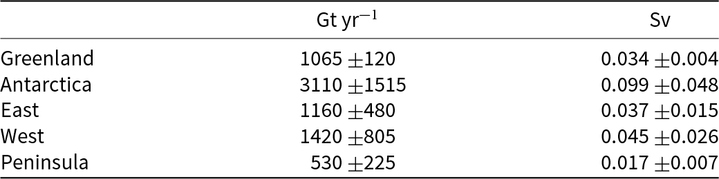
All mass flow terms and values for each term are shown in Tables 1 and 2 and the Sankey diagrams. In addition, the tables contain the time span of each value and reference publication. Net freshwater mass flow rates are shown in Table 3 and net mass loss by region and grounded vs floating ice are shown in Table 4.
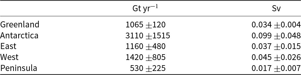
Net freshwater export mass flow rate for Greenland, Antarctica, and Antarctic regions in Gt yr $^{-1}$ and Sverdrup (106 m3 s $^{-1}$).
Net mass change flow rate and uncertainty. Grounded, floating, and total columns are estimates from this paper. Uncertainty estimates come from a GMB uncertainty assessment described by Groh and others (Reference Groh2019).

4.1. Freshwater mass flow rate
Net freshwater export to the ocean (mass loss terms excluding sublimation and evaporation) is 1065  $\pm$120 Gt yr $^{-1}$ for Greenland and 3110 $\pm$1515 Gt yr $^{-1}$ for Antarctica. Antarctic sub-region values are also provided in Table 3, along with values in Sverdrup or 106 m3 s $^{-1}$.
4.2. Mass change
Mass change for the 2010 through 2019 period is net mass loss for Greenland, West Antarctica, the Antarctic Peninsula, and Antarctica as a whole, but net mass gain in East Antarctica (Table 4).
Greenland lost 255  $\pm$40 Gt yr $^{-1}$ from grounded ice and an additional 75 $\pm$10 Gt yr $^{-1}$ (30%) from floating ice.
Antarctica lost 190  $\pm$115 Gt yr $^{-1}$ from grounded ice and an additional 260 $\pm$155 Gt yr $^{-1}$ ( $\sim$140%) from floating ice. The grounded ice mass loss is partitioned with 250 $\pm$190 Gt yr $^{-1}$ lost from West Antarctica and 20 $\pm$10 Gt yr $^{-1}$ lost from the Peninsula offset by 80 $\pm$50 Gt yr $^{-1}$ gained in East Antarctica. Floating ice mass losses are partitioned with 275 $\pm$190 Gt yr $^{-1}$ lost from West Antarctica and 175 $\pm$85 Gt yr $^{-1}$ lost from the Peninsula offset by 190 $\pm$115 Gt yr $^{-1}$ gained in East Antarctica.
In comparison, estimated net grounded ice mass loss by the GMB method is 226  $\pm$15 Gt yr $^{-1}$ (we round this uncertainty up to 10% in Table 4) in Greenland (Döhne and others, Reference Döhne, Horwath, Groh and Buchta2023) and 151 $\pm$44 Gt yr $^{-1}$ ( $\sim$30%) in Antarctica (Groh and Horwath, Reference Groh and Horwath2021). The Antarctic regions have uncertainty of 115%, 10%, and 35% for the East, West, and Peninsula respectively.
5. Discussion
5.1. Constituent terms and net versus gross
We recommend to the community to report all the constituent terms of mass change as well as the gross values, and not only the net values. If needed, it is relatively straightforward to include a net combined term. There are numerous advantages to this approach. More information is better. Constituent term level details are needed to properly quantify and attribute differences in SMB model inter-comparison studies (e.g., Mottram and others, Reference Mottram2021). The potential benefits for future researchers to address currently-unknown research questions or undefined needs is likely to outweigh the costs of increased complexity, time, storage, and access.
We do show some net terms here in the graphics when we combine frontal retreat, frontal advance, calving, and frontal melt in the case of Greenland, because frontal advance is not a mass gain term. However, in Tables 1 and 2 we report gross terms as provided by the upstream data products.
Sea level rise research often focuses on how and why, not only how much. Process level detail is needed to provide model inputs or validation for the how and why. However even the IO method that provides process level detail is usually estimated with a single SMB value rather than constituent terms as shown here, and may miss important information. For example, if net SMB remains constant over time, but snowfall and runoff both increase, this indicates a different ice sheet state, and this information should not be removed through reporting of net values.
The largest input, by far, is snowfall in Antarctica. Unfortunately, this process involves integrating small values over a large area, which introduces high uncertainty. The second largest term in Antarctica is calving, but unlike snowfall this occurs in large quantities from just a few ice shelves. Continued production, maintenance, and improvement of these datasets to generate robust time series is essential for monitoring ice sheet health and improving our understanding of processes contributing to sea level rise.
Finally, although we argue for gross, not net, and inclusion of constituent terms in general when sharing outputs, we caution that any users should consider if this is the correct treatment for their application. As discussed in the Methods, use cases should carefully consider assumptions of tracer treatment, for example, if a tracer is not conserved during a freeze-then-melt cycle. By providing constituent and gross terms, we hope this data set is still useful for these scenarios.
5.2. Net mass loss and gain
We have been using the terms ‘mass loss’ vs ‘mass gain’ or ‘drawdown or retreat’ vs ‘build-up or expansion.’ The specific cause of these processes can be thought of as a recursive application of the methods, tables, and graphics here. That is, the imbalance is due to changes from some balanced baseline and the changes are likely all of the terms here – decreases or increases of inputs offset by decreases or increases of outputs.
For example, the ‘mass loss’ input in Fig. 1 could be an inset Sankey diagram showing changes in all of the terms relative to some steady state baseline. Similarly, the value in a table for a ‘mass loss’ key could be a single value, or a nested table showing all the terms that contribute to that value.
5.3. Freshwater export, mass loss, and anomalies
Oceanographic models often use ice sheet freshwater export as a forcing, but it can be challenging for those model developers to find appropriate inputs in part because some models are coupled to ice sheet models, or global climate models with ice sheets, that contain some but not all processes. Ocean models and modelers then need to understand what processes are and are not included in the ice sheet outputs, and for the processes that are included, they may need to determine the anomalies and then add that to the ocean model (cf. Schmidt and others, Reference Schmidt2025).
The smaller terms shown here (e.g., grounded ice basal melt from either ice sheet, Greenland frontal retreat, grounding line retreat, basal melt, etc.) are commonly excluded because they are small, but ocean modelers who work with anomalies should be careful of excluding these small terms. These smaller terms are also often less likely to be included in the ice component driving or coupled to the ocean model. Their inclusion should be considered, if appropriate, in the ocean model because these small processes can match the magnitude of the anomaly, especially if several of the smaller terms are combined.
5.4. Uncertainty
Uncertainty on the derived mass loss and mass gain terms is difficult to quantify because these terms are residuals – the small difference of several large numbers, some with large uncertainty. This is one of the major weaknesses of the IO method which is primarily used here. A basic uncertainty propagation could assume each term is independent (they are not) and report the residual values of mass loss and gain as the square root of the sum of the square of the individual uncertainty estimates. This calculation is trivial and this method produces a number, but it is unreasonably large.
A comparison of the estimated net grounded ice mass loss with results of the independent GMB method (Table 4) indicates a much better agreement between the two methods than suggested by a basic uncertainty propagation of all IO terms. The independently assessed uncertainty for the GMB method better fits to the differences in estimates for all regions under investigation (e.g., for Antarctica the difference between the two methods is 39 Gt yr $^{-1}$ and the uncertainty of the GMB estimate is 45 Gt yr $^{-1}$). Using the GMB uncertainty as our derived residual uncertainty may be appropriate, and would provide a much smaller uncertainty than the values we report here. However, we only use the GMB uncertainty to provide context because there is no physical basis and mathematical connection between the mass change estimates (residual from the IO method) and the mass change uncertainty (from the GMB method).
5.4.1. Greenlandic discharge, calving, and frontal melt uncertainty
Discharge uncertainty in Greenland is reasonably well constrained at  $\sim$10% by Mankoff and others (Reference Mankoff, Solgaard, Colgan, Ahlstrøm, Khan and Fausto2020b) and other similar products.
The division of discharge when it is divided into submarine melt and calving is highly uncertain. Rignot and others (Reference Rignot, Koppes and Velicogna2010) reports ‘we conclude from this comparison that 20–80% of the summer ice-front fluxes are directly melted by the ocean’ with the remainder coming from calving. But that study only examined a few glaciers for a relatively short period of time. From this, we split discharge 50/50 between frontal melt and calving (see Methods), and assign an uncertainty of 30%. However, in this case, the two terms are not independent. They are highly dependent, constrained by the upstream discharge with 10% uncertainty. It is only the separation and form or phase (solid or liquid) that is highly uncertain.
5.4.2. Antarctic Discharge
Discharge and discharge uncertainty in Antarctica is challenging to quantify. At the low end, Rignot and others (Reference Rignot, Mouginot, Scheuchl, van den Broeke, van Wessem and Morlighem2019) reports uncertainty of  $\sim$5% on the discharge term. This seems unlikely for several reasons, including that discharge uncertainty in Greenland is more than 5% and bed topography – the main source of discharge uncertainty – is better constrained there, or that Rignot and others (Reference Rignot, Mouginot, Scheuchl, van den Broeke, van Wessem and Morlighem2019) calculates discharge using a corrective scaling factor ranging from 0.62 to 4.57 and relies on 5 separate methods (that are applied in isolation, not constraining each other).
At the high end, Davison and others (Reference Davison2023) report a cumulative discharge (from grounded ice to ice shelves) change of 1770  $\pm$870 Gt which is $\sim$50%, but Antarctic-summed steady state discharge of $\sim$1840 $\pm$
$\pm$ $\sim$125 Gt yr $^{-1}$ which is $\sim$5%.
5.5. Missing terms, limitations, and simplifications
These figures and tables neglect some mass flow processes (some of which are included in Cogley and others (Reference Cogley2011, Fig. 2), and simplify others.
Neglected processes include grounded ice basal freeze-on (cf. Bell and others, Reference Bell2014). Grounded ice basal melt estimates currently assume all melt leaves the ice sheet and is therefore mass loss. That seems unlikely, given both observations of freeze-on (Bell and others, Reference Bell2014) and that some melt, especially from the geothermal term (cf. Karlsson and others, Reference Karlsson2021) occurs under thick ice far inland and far from active subglacial conduits. That is, there should be a separate term and second ‘refreezing’ loop at the bottom of the Sankey diagrams to represent basal refreezing.
Similarly, englacial storage may modify the runoff term. Steady state englacial storage does not modify the magnitude, but does impact the timing of runoff, which does not change these decade-scale Sankey diagrams, but would change seasonal scale diagrams. If englacial storage changes magnitude in either direction, this has a direct impact on runoff magnitude.
Sub-aqueous frontal melt is excluded in Antarctica, because it is usually excluded in the literature that focuses on ice shelf basal melt or calving. This term is implicitly included in the calving estimates. This process remains unquantified on ice-sheet wide scales.
Subaerial frontal melt and sublimation of the vertical face above the water line Cogley and others (Reference Cogley2011, Fig. 2) is not explicitly treated but is included in other terms.
Grounding line retreat in both Greenland and Antarctica is largely unquantified in the units needed to include it here, as discussed in the methods.
We neglect avalanche on and off ice sheets – these likely matter more for mountain glaciers.
Snow drift on and off is also excluded. There is likely little snow drift onto either ice sheet, but drifting off may be of similar magnitude to some of the other smaller terms shown here.
This work focuses on Greenlandic and Antarctic ice masses as a freshwater source. There are other sources and sinks of freshwater into the oceans around Greenland and Antarctica not covered here, including but not limited to: rain and snow melt from non-ice covered ground in Greenland (Mankoff and others, Reference Mankoff2020a), rain and snow directly onto the fjord or ocean surface, evaporation over the surrounding oceans, and sea ice growth, movement, and melt.
There are a variety of simplifications. For example, not all rainfall input turns to ice as depicted by the arrows in these diagrams. Some enters as part of the refreezing loop, and some remains liquid and leaves as runoff or evaporation. Similarly, the evaporation output could pull from the refreezing loop (in the liquid phase, depicted by the blue color) and also directly from rainfall as stated above. Although some path details are simplified, the magnitudes are still as reported in the input products. Furthermore, the simplifications we are aware of are all a very small component relative to the total freshwater or mass flow or even the mass imbalance.
5.5.1. Temporal resolution of input observations
The value of some terms presented here are biased by the temporal resolution of the upstream product that is an input to this work. This is the case for all terms until the observations are instantaneous, but impacts bi-directional processes like advance and retreat or step change processes like calving more than slowly varying processes like discharge. For example, in Greenland we report 50 Gt yr $^{-1}$ frontal retreat and 0 Gt yr $^{-1}$ frontal advance using decade-scale reporting from Kochtitzky and others (Reference Kochtitzky2023). However, that is a decadal net term despite the majority of this work reporting gross terms, and sub-decadal advances are not captured there.
Given a theoretical reference front location for calving and frontal melt,  $X$ Gt of frontal retreat may actually be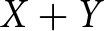 $X + Y$ Gt frontal retreat offset by $Y$ Gt frontal advance that occurred at a temporal resolution below the observations. This does not matter for total freshwater mass which should be calculated using net frontal change, not gross frontal retreat. Ice shelf basal freeze-on and melt share some similar temporal resolution dependent issues, and a decision to use net or gross is dependent on the use case.
6. Summary
Previous estimates of mass loss for Greenland and Antarctica show a range of values (Otosaka and others, Reference Otosaka2023), highlighting the need for improved estimates and a common framework for accounting of ice sheet mass balance. The work presented here offers one such framework that could be adopted by the community for future balance estimates.
In this work we report total ice sheet and peripheral glacier mass change for both Greenland and Antarctica for the 2010 through 2019 period, reporting not just grounded ice mass loss, but also changes in floating ice. We have provided all available constituent terms and gross not net values. This detailed information provides a better picture of ice sheet health than focusing only on mass loss or only on grounded ice.
We have also displayed these constituent terms and net values using Sankey diagrams which provide an information-dense display showing (a) the relations between terms and processes, (b) quantitative display of the magnitude of each term, and (c) visual comparisons between different ice sheets or sub-regions of ice sheets, as the magnitude of the graphic uses the same proportion between all images.
Data availability
Data and source code used to generate the Sankey diagrams in this paper can be found on https://doi.org/10.5281/zenodo.15819650.
Acknowledgements
We thank Andreas Ahlstrøm and Nanna Karlsson for additional comments on this paper, and Kristin Poinar for suggesting improvements to the Sankey figure. We thank Aman KC and two additional reviewers for their comments that helped improve the manuscript. We also thank Gaborit (Reference Gaborit2021) for the LaTeX TikZ Sankey package, and Cogley and others (Reference Cogley2011) for a reference graphic. Analysis was aided by the software packages Pandas (The pandas development team, 2020), GeoPandas (den Bossche and others, Reference den Bossche2024), Xarray (Hoyer and Hamman, Reference Hoyer and Hamman2017), and GRASS GIS (GRASS Development Team, 2018), among other tools.
Author contributions
Author contributions following theCRediT system (Allen and others, Reference Allen, Scott, Brand, Hlava and Altman2014; Reference Allen, O’Connell and Kiermer2019; Brand and others, Reference Brand, Allen, Altman, Hlava and Scott2015): KDM: data, graphic, write, edit, discuss; CAG, BD, TD: data, edit, discuss; DT, WK, ASG: edit, discuss; XF: data, discuss; DR: graphic, discuss; CQK, GW, BVL: data; RF: discuss.
Funding statement
Ken Mankoff was supported by the NASA Goddard Institute for Space Studies (GISS) and the NASA Modeling, Analysis and Prediction program. Alex Gardner and Chad Greene contributions were carried out at the Jet Propulsion Laboratory, California Institute of Technology, under a contract with the National Aeronautics and Space Administration (80NM0018D0004). The work of Thorben Döhne was funded by the European Space Agency through the Climate Change Initiative (CCI) projects Antarctic Ice Sheet CCI+ (Contract Number 4000126813/19/I-NB) and Greenland Ice Sheet CCI+ (contract number and 4000126523/19/I-NB).
Competing interests
No authors have any conflict of interest with the work presented here.
Appendix A. Sankey diagram tools
There are several software packages that support creating Sankey diagrams with various levels of complexity and control. The four applications we found, in order from easiest and most limited to most complex and feature-full are the Mermaid diagram tool, Plotly (which can be used from Python, R, or other popular languages), Matplotlib, and finally LaTeX.
The simplest Mermaid option is produced with only a CSV file of the format ‘in,out,value’. Neither order nor closure (balance) is important, and a user has limited control over layout and color, although a user can edit things later manually if generating SVG format. We used Mermaid to generate the Sankey diagram in Fig. 4, and the source for these diagrams can be found in the available data repository at https://doi.org/10.5281/zenodo.15819650 file mermaid.org. Mermaid diagrams in Markdown files on GitHub render directly in the browser from the data (no saved image file).
The main Sankey diagrams shown here are generated using a LaTeX template that uses the TikZ Sankey package (Gaborit, Reference Gaborit2021). We use a script that inserts CSV tables into the template. This architecture makes it trivial to generate similar diagrams for other time periods (e.g., a Sankey diagram per year), differences between time periods, other regions (e.g., one diagram per glacier basin), etc.












 Open access

