


1 Introduction
Political science that leverages machine learning is becoming ubiquitous. Scholars encourage exploration of these methods, particularly using textual data (Wilkerson and Casas Reference Wilkerson and Casas2017). Examples include analyzing sentiment of parties in parliamentary debates or Twitter users (Castanho Silva and Proksch Reference Castanho Silva and Proksch2022; Tumasjan et al. Reference Tumasjan, Sprenger, Sandner and Welpe2010), as well as topic modeling for studying agenda setting, political attention, or news (Barberá et al. Reference Barberá2019, Reference Barberá, Boydstun, Linn, McMahon and Nagler2021; Quinn et al. Reference Quinn, Monroe, Colaresi, Crespin and Radev2010). The “text-as-data” paradigm has been a reality for at least a decade. While such techniques should augment rather than replace humans (Grimmer and Stewart Reference Grimmer and Stewart2013), they enable the exploration of political content at scales previously unimaginable.
A significant portion of content consumed today (whether political or otherwise) is audiovisual. The rise of media platforms, such as Instagram, TikTok, YouTube, and podcasts, contrasts with text-centric formats like Twitter/X or Reddit, stressing the need for research engaging these modalities. In political contexts, text is often assumed to carry the bulk of meaning, but nonverbal elements offer insights lost in transcript-only analysis. Audio captures intonation, pitch, and emotion; video reveals body language, facial expressions, and visual cues. In presidential debates, nonverbal behaviors displaying hostility or anger are more frequent than verbal character attacks or angry language, and correlate with responses in social media (Bucy et al. Reference Bucy2020).
As text as data has advanced in political science, multimodal analysis remains relatively underdeveloped. Challenges preventing uptake include the skillset to analyze these other modalities of data, from signal processing techniques for audio files, to computer vision techniques for video sources. Here, we provide a comprehensive introduction to foundational techniques for audio analysis, showcasing practical examples and case studies in computational political science. Our point of entry opens opportunities for more advanced methods, such as deep learning-based speech recognition and emotion detection. We aim to make audio data more accessible within political science, encouraging scholars to expand their methodological toolkit. Audio analysis can enrich our understanding of political dynamics, providing a fuller picture of the complex nature of political communication.
2 Beyond Text: Audio as Data and the “Alignment Crisis”
Ensuring validity and robust standards requires responsibly leveraging new data opportunities (Wilkerson and Casas Reference Wilkerson and Casas2017). Audio, images, and video have slowly emerged in political science thanks to machine learning technologies like convolutional neural networks (CNNs; Torres and Cantú Reference Torres and Cantú2022). Cantú (Reference Cantú2019) identified the alteration of vote-tally sheets during the 1988 Mexican presidential election from an image database. Boussalis et al. (Reference Boussalis, Coan, Holman and Müller2021) presented the first study employing multimodal methods of emotion detection to investigate congruency of gender with emotional expression and vocal pitch in German national leadership and minor party debates, finding that Angela Merkel was punished for showing anger and rewarded for expressing happiness. Similarly, Shah et al. (Reference Shah2024) developed a multimodal classifier, integrating video, audio, and text to detect aggressive behaviors in U.S. presidential debates.
A parallel line of work explores audio in political speech—what might be called the “audio-as-data” paradigm (Dietrich, Enos, and Sen Reference Dietrich, Enos and Sen2019; Dietrich, Hayes, and O’Brien Reference Dietrich, Hayes and O’Brien2019; Knox and Lucas Reference Knox and Lucas2021; Proksch, Wratil, and Wäckerle Reference Proksch, Wratil and Wäckerle2019; Rittmann Reference Rittmann2024). Klofstad (Reference Klofstad2016) investigated the effect of voice pitch of political candidates on voters, finding lower-pitched voices associate with perceived electoral success, particularly among male candidates. Damann, Knox, and Lucas (Reference Damann, Knox and Lucas2025) challenged assumptions in text as data by showing that vocal delivery, including pitch and volume, shapes perceptions of traits like competence and passion. Crucially, they found these features rarely vary in isolation—speech modulation and other complex patterns often matter more than reductive metrics like pitch.
The Oyez project, providing aligned transcripts from the U.S. Supreme Court, was used by Knox and Lucas (Reference Knox and Lucas2021) to model “judicial skepticism,” a feature not easily captured through text alone. The authors relied on time stamps to split their data into utterances and then validate with text-based models (which performed poorly, as they cannot capture this auditory subtlety). Dietrich, Enos, and Sen (Reference Dietrich, Enos and Sen2019) used the same dataset to analyze emotional arousal, showing that vocal features can predict voting behavior. Dietrich, Hayes, and O’Brien (Reference Dietrich, Hayes and O’Brien2019) used data from HouseLive, a service that provides live and archived videos of the U.S. House of Representatives, to analyze vocal pitch and emotional intensity of congressional speech, again finding gendered differences in references to women. More recently, Rittmann (Reference Rittmann2024) replicated this finding in the German Parliament, helping rule out through replication reasonable doubts that differences in emotional intensity are confounded by national or institutional variables like incentives to cultivate personal votes and party discipline.
These examples were possible thanks to the alignment between text and audio, but such resources are scarce. Alignment at source requires resource. Most political speeches are not backed up by large institutions, such as the Office of the Clerk for HouseLive, and only provide transcripts or audio. In the United Kingdom, Hansard provides full transcripts from the House of Commons and the Lords, and ParliamentTV provides videos dating back to 2007. Unfortunately, these are not reliably aligned at the utterance, only at the session level. ParliamentTV also limits downloads, hampering automated collection.
To solve this “alignment crisis,” in which huge corpora of textual, auditory, and visual data are co-existing but not intersecting, Proksch, Wratil, and Wäckerle (Reference Proksch, Wratil and Wäckerle2019) evaluated automatic speech recognition (ASR), noting that ASR has greatly improved since the 1990s, with Google’s ASR reaching a word error rate (WER)Footnote 1 of 0.05. As the authors caution, these validations are performed in laboratory conditions and do not account for levels of noise or crosstalk often present in political speech. Using the European Union State of the Union corpus for English, they find WER of 0.03 with the YouTube API and 0.21 with the Google API, with generally worse results for other languages, ranging from WER of 0.10 to 0.26 for French and German. They demonstrate that “automatic transcription tools have reached accuracy levels that make them useful for the study of parliamentary debates, campaign speeches, and intergovernmental deliberations” (Proksch, Wratil, and Wäckerle Reference Proksch, Wratil and Wäckerle2019, 357). However, they report that APIs performed differently depending on clip length and warn about legal issues related to data protection, as copies of the audio files are sent to YouTube or Google servers.Footnote 2 Recent sophisticated models, like OpenAI’s Whisper, have been analyzed for accent and speaker differences. Graham and Roll (Reference Graham and Roll2024) found Whisper performed best for U.S. and Canadian accents but poorly for Vietnamese and Thai accents in English, and for native but regional accents, such as the British Leeds accent, with a match error rate (MER)Footnote 3 of almost 100%.
Our paper advances this conversation by addressing alignment, feature extraction, and classification of speech and emotion using modern audio embeddings. As a case study, we analyze televised U.S. presidential debates since first airing in 1960, until 2020, including vice-presidential debates. We obtained 47,150 sentences from the debate transcripts (38,649 from candidates and 8,501 from moderators, panelists, or audience members) initially unaligned to their respective videos. We obtained 243,023 s or 4,050 min or 67.5 h across 45 videos. In these videos, 34 candidates (16 democrats, 15 republicans, and 3 independent), 82 moderators and panelists, and 59 audience members appeared.
We begin by explaining core audio concepts relevant to political scientists (Section 3). We present four progressive applications to demonstrate ways of leveraging audio data for political science research, namely audio-text forced alignment (Section 4.1), analysis of individual speaking styles using low-level features (Section 4.2), construction of custom-made machine learning models for classification tasks (Section 4.3), and off-the-shelf machine learning models for emotion recognition (Section 4.4). We provide all replication codes in Python, transcripts, alignment data, and results in the Dataverse record Mestre and Ryan (Reference Mestre and Ryan2025) as well as our GitHub: https://github.com/rafamestre/audio-as-data.Footnote 4
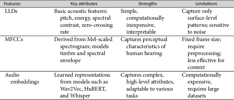
To fully understand the affordances of audio as data, it is necessary to appreciate the complex and multidimensional nature of audio signals. In speech processing and recognition, several features distinguish various aspects of audio signals. We explore two classical audio feature sets, low-level descriptors (LLDs) and Mel-frequency cepstral coefficients (MFCCs), as well as novel audio embeddings, which attempt to capture multidimensional representations of audio signals, discerning patterns, and relationships in a way akin to word embeddings. Table 1 introduces features’ key attributes, strengths, and limitations.
Summary of audio feature extraction techniques.

Table 1 Long description
The table consists of four columns: Features, Key attributes, Strengths, and Limitations.
* Row 1: Features is L L Ds. Key attributes include basic acoustic features like pitch, energy, spectral contrast, and zero-crossing rate. Strengths are listed as simple, computationally inexpensive, and interpretable. Limitations are that they capture only surface-level patterns and are sensitive to noise.
* Row 2: Features is M F C C s. Key attributes are derived from Mel-scaled spectrogram and models timbre and spectral envelope. Strengths include capturing perceptual characteristics of human hearing. Limitations include fixed frame size, requirement for preprocessing, and being less effective for context.
* Row 3: Features is Audio embeddings. Key attributes are learned representations from models such as Wav2Vec, HuBERT, and Whisper. Strengths are capturing complex, high-level attributes and adaptability to various tasks. Limitations are being computationally expensive and requiring large datasets.
Footnote: Abbreviations include L L D for low-level descriptor and M F C C for Mel-frequency cepstral coefficient.
Abbreviations: LLD, low-level descriptor; MFCC, Mel-frequency cepstral coefficient.
3 Understanding Audio Features
An audio signal is a series of air vibrations measured over time. Its typical representation is a waveform like Figure 1a, which shows the amplitude (or strength) of vibrations at each point in time. This time-based view reveals little about the nature of the sound. Speech, music, or noise may look similar in waveform form but differ significantly in content. We often transform the signal into the frequency domain, producing a spectrogram (Figure 1b).
Representation of an utterance in different modalities. (a) As a discrete mathematical function with an amplitude changing over time. (b) As a spectrum of energy in decibels with respect to time.

Figure 1 Long description
Panel a is a waveform line graph. The x-axis is Time in seconds s, ranging from 0 to 4. The y-axis represents amplitude. The data shows a series of irregular black vertical spikes and clusters representing sound pressure over time, with distinct bursts of activity followed by brief periods of lower amplitude.
Panel b is a Mel spectrogram heat map. The x-axis is Time in seconds s, ranging from 0 to 3.5. The y-axis is Frequency in H z, with logarithmic labels at 0, 512, 1024, 2048, and 4096. A color scale on the right indicates energy in d B, ranging from minus 80 d B in black to 0 d B in light yellow. The plot shows bright horizontal bands and vertical structures concentrated below 1024 H z, indicating higher energy at lower frequencies, with periodic vertical striations corresponding to the rhythmic nature of the utterance.
The y-axis represents the signal frequency and the z-axis (color bar) how much energy is present at each frequency over time. This spectral view decomposes the signal into a combination of simple waves at varying frequencies and amplitudes, making it more analytically useful.
3.1 Low-Level Descriptors
Derived from spectral representations, LLDs describe basic properties of an audio signal and serve as inputs for more complex feature extraction. Typical LLDs include root-mean-squared energy (also known as loudness or intensity), pitch, spectral contrast, spectral flux, zero-crossing rate, and various spectral shape descriptors, such as spectral centroid, spread, skewness, and kurtosis. We explore two of the most important LLDs for speech analysis: energy and pitch.
Energy refers to the loudness or intensity of an audio signal. Mathematically, for a discrete-time signal $x\left[n\right]$
of duration
$x\left[n\right]$
of duration $T$
, discretized into
$T$
, discretized into $N$
points, and sampled at a rate/frequency
$N$
points, and sampled at a rate/frequency ${f}_s=N/T,$
the energy is calculated as
${f}_s=N/T,$
the energy is calculated as $E=\sum_{n=0}^{N-1}{x}^2\left[n\right].$
This measure quantifies the “power” or “volume” of the signal, capturing the total magnitude of the sound waves, and is important for voice activity detection systems that identify when someone speaks.
$E=\sum_{n=0}^{N-1}{x}^2\left[n\right].$
This measure quantifies the “power” or “volume” of the signal, capturing the total magnitude of the sound waves, and is important for voice activity detection systems that identify when someone speaks.
The pitch, or fundamental frequency, ${F}_0$
, has already been shown to correlate with the speaker’s emotional state (Dietrich, Hayes, and O’Brien Reference Dietrich, Hayes and O’Brien2019). Pitch refers to the perceived frequency of a sound and varies with both emotion and linguistic function. For instance, in tonal languages like Mandarin, pitch distinguishes meaning between similar words. In other languages, a change in pitch at the end of the sentence indicates a question. A higher-than-usual pitch might indicate excitement or anger, whereas a lower pitch can indicate calmness. Mathematically, pitch can be calculated using several methods, which include the YIN algorithm (de Cheveigné and Kawahara Reference de Cheveigné and Kawahara2002) and probabilistic YIN (pYIN; Mauch and Dixon Reference Mauch and Dixon2014), among others.
${F}_0$
, has already been shown to correlate with the speaker’s emotional state (Dietrich, Hayes, and O’Brien Reference Dietrich, Hayes and O’Brien2019). Pitch refers to the perceived frequency of a sound and varies with both emotion and linguistic function. For instance, in tonal languages like Mandarin, pitch distinguishes meaning between similar words. In other languages, a change in pitch at the end of the sentence indicates a question. A higher-than-usual pitch might indicate excitement or anger, whereas a lower pitch can indicate calmness. Mathematically, pitch can be calculated using several methods, which include the YIN algorithm (de Cheveigné and Kawahara Reference de Cheveigné and Kawahara2002) and probabilistic YIN (pYIN; Mauch and Dixon Reference Mauch and Dixon2014), among others.
Other LLDs, such as zero-crossing rate (the frequency of sign changes in the waveform), spectral flux (changes in the power spectrum over time), and spectral contrast (variation in energy across frequency bands), can support speech analysis by capturing subtle aspects of sound texture. While they are more commonly used in music or linguistic research, they may also offer insights into political speech, such as distinguishing phonetic features or prosodic patterns.
3.2 Mel-Frequency Cepstral Coefficients
MFCCs are widely used in speech and audio processing to represent the spectral shape of an audio signal based on human hearing perceptions, making MFCCs particularly useful for speech recognition and classification tasks. The process of obtaining MFCCs involves several complex transformations, which we briefly outline here (see Supplementary Appendix A for a detailed walkthrough).
First, some preprocessing is performed on the discrete signal $x\left[n\right]$
, where
$x\left[n\right]$
, where $n\in \left[0,N-1\right]$
, sampled at rate
$n\in \left[0,N-1\right]$
, sampled at rate ${f}_s.$
The signal is pre-emphasized by amplifying higher frequency regions, particularly around 1–5 kHz, where our hearing system is more sensitive (Picone Reference Picone1993). The signal is then divided into short overlapping frames or segments of approxmately 20–40 ms. This framing is done because frequencies change over time, and we wish to analyze the frequency spectrum at a specific time a sound is produced. This approach assumes that in each short segment, the voice has stationary acoustic features. Finally, the signal is windowed using a Hamming functionFootnote 5
that reduces the amplitude at the extremes, producing a cleaner frequency spectrum.
${f}_s.$
The signal is pre-emphasized by amplifying higher frequency regions, particularly around 1–5 kHz, where our hearing system is more sensitive (Picone Reference Picone1993). The signal is then divided into short overlapping frames or segments of approxmately 20–40 ms. This framing is done because frequencies change over time, and we wish to analyze the frequency spectrum at a specific time a sound is produced. This approach assumes that in each short segment, the voice has stationary acoustic features. Finally, the signal is windowed using a Hamming functionFootnote 5
that reduces the amplitude at the extremes, producing a cleaner frequency spectrum.
Next, we apply a fast Fourier transform (FFT) on the preprocessed signal. The FFT yields a frequency-domain representation, showing the signal’s main constituent frequencies. This transformation allows us to examine how energy is distributed across different frequency bands within each frame. A speaker with a higher pitch will show greater energy in higher-frequency regions, whereas a speaker with a lower pitch will concentrate more energy in lower frequencies. A certain and unique distribution of frequencies characterizes not only the speaker but also the sounds they were making in that short interval.
Human hearing perceives frequencies approximately linearly below 1 kHz and logarithmically above (Stevens and Volkmann Reference Stevens and Volkmann1940). To reflect this perceptual nonlinearity, the Mel scale is used and calculated as follows:
 $$\begin{align}{f}_{\mathrm{Mel}}=2595\cdotp {\log}_{10}\left(1+\frac{f}{700}\right).\end{align}$$
When plotted, this Mel scale increases almost linearly until 1,000 Hz, then logarithmically. The frequency spectrogram is nonlinearly transformed using the Mel scale to obtain a more meaningful representation of each sound and simulate our hearing perceptions: with lower frequencies being more discernible but higher frequencies more averaged out. This produces a Mel spectrogram, as shown in Figure 1b, where the frequencies in the y-axis follow a nonlinear scale shaped by perceptual sensitivity. After some postprocessing, each time frame is summarized as a set of $c\left[n\right]$
MFCC coefficients per time window, which effectively compress the raw audio into a set of frequency features aligned with human hearing perceptions.
$c\left[n\right]$
MFCC coefficients per time window, which effectively compress the raw audio into a set of frequency features aligned with human hearing perceptions.
3.3 Audio Embeddings
Deep learning allows the extraction of data-driven high-level features or embeddings from audio data. Unlike LLDs and MFCCs, embeddings capture abstract audio characteristics that are challenging to engineer manually. Models such as HuBERT and Wav2Vec are among the most widely used.
Wav2Vec (Schneider et al. Reference Schneider, Baevski, Collobert and Auli2019), or recently Wav2Vec 2.0 (Baevski et al. Reference Baevski, Zhou, Mohamed and Auli2020), is a self-supervised learning approach developed by Facebook AI that learns embeddings from raw audio data. The model uses convolutional layers to create a sequence of embeddings, masking part of the input and predicting it from the unmasked context. These feature vectors are then contextualized via a transformer model like those used in natural language processing (NLP), such as BERT (Bidirectional Encoder Representations from Transformers). For political scientists studying speech, Wav2Vec 2.0 provides comprehensive, high-level embeddings that capture a variety of speech attributes, which can be fine-tuned for tasks like speaker identity, emotion (Pepino, Riera, and Ferrer Reference Pepino, Riera and Ferrer2021), and even extracting some semantic content from spoken words.
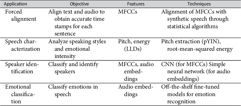
While LLDs and MFCCs offer low-level, signal-based features that are typically language-agnostic, audio embeddings are often trained on specific languages and may not generalize well across languages, accents, or cultural contexts. Though large models like Wav2Vec 2.0 also have fine-tuned multilingual variants, their application can be computationally expensive for the average user. “Basic” features such as MFCCs and LLDs can still be extremely attractive for tasks that do not require uncovering complex relationships in speech. We now showcase four applications summarized in Table 2, where each of these classes of features can be useful.
Overview of applications and techniques presented in this work.

Table 2 Long description
The table consists of four columns and four rows of data.
Row 1: Application is Forced alignment. Objective is to align text and audio to obtain accurate time stamps for each sentence. Features used are M F C C s. Techniques involve alignment of M F C C s with synthetic speech through statistical algorithms.
Row 2: Application is Speech characterization. Objective is to analyze speaking styles and emotional intensity. Features are Pitch and energy L L D s. Techniques include pitch extraction p Y I N and root-mean-squared energy.
Row 3: Application is Speaker identification. Objective is to classify and identify speakers. Features are M F C C s and audio embeddings. Techniques include C N N for M F C C s and a simple neural network for audio embeddings.
Row 4: Application is Emotional classification. Objective is to classify emotions in speech. Features are audio embeddings. Techniques involve off-the-shelf fine-tuned models for emotion recognition.
Abbreviations: CNN, convolutional neural network; LLD, low-level descriptor; MFCC, Mel-frequency cepstral coefficient.
4 Four Applications
The transcripts for this study were collected from the website of the Commission for Presidential Debates originally by the team behind the USElecDeb60To16 dataset (Haddadan, Cabrio, and Villata Reference Haddadan, Cabrio and Villata2020). We reused this open-source dataset, expanded it to include presidential debates from 2020, and fixed some sentence omissions. Videos were downloaded from the YouTube channel of the Commission for Presidential Debates. The first challenge is to get accurate time stamps that match each sentence to a time segment in the audio files.
4.1 Forced Alignment with MFCCs
Here, we present the forced alignment solution to illustrate the application of MFCCs in a typical case where both text and audiovisuals come from different sources. While ASR might produce highly accurate results in terms of word recognition, in our case, high quality transcripts developed by skilled humans were already available. Using those is preferable as they should be more accurate than automatically generated transcripts.Footnote 6 For researchers interested in sociolinguistics, forced alignment can also be used to match phonemes and closely study languages or dialects. However, when transcripts are unavailable or of lower quality, then ASR might be the technique of choice for obtaining time-stamped transcripts and performing audio–textual analysis of speeches.
Aeneas is a forced alignment technique that uses artificial voices to match sets of MFCCs through the statistical algorithm of dynamic time warping. This approach was applied to each debate, and the results were evaluated using crowdsourced annotations from a randomly selected subset of 500 utterances. Supplementary Appendix B presents an overview of forced alignment techniques used in the literature, and Supplementary Appendix C provides more specific details on aeneas.
Each utterance was annotated five times for robustness. In the evaluation process, we presented annotators with pairs of audio and text that had undergone alignment. They were asked to rate the alignment quality on a scale of 1 (not aligned at all) to 5 (perfect alignment). We defined two alignment metrics: the percentage agreement (PA) measure, which amounted to 85.26%, and the distance-based agreement (DA) measure to quantify the extent of any (dis)agreement, which was 95.76%. Full details and definitions of these metrics are in Supplementary Appendix D. Both measures, particularly the latter, indicate a significant degree of consistency among the crowd annotators. The DA measure, being approximately 10 percentage points higher than the PA, implies that while the annotators disagreed on few ratings, discrepancies that arose were minor, likely attributable to the inherent subjectivity of the continuous rating scale.
As depicted in Figure 2a, the average rating reveals that most annotations scored 5 in a 1–5 rating scale, indicating perfect alignment. Only 5% of text–audio pairs were deemed “not aligned at all.” To investigate, we hypothesized the mismatch was attributable to some sentences being exceptionally short, comprising expressions such as “okay” or “yes.” When plotting the average sentence length per rating in Figure 2b, we noticed a distinct trend where short sentences were commonly deemed poorly aligned. Longer sentences provide more accurate time stamps, whereas shorter or interrupted sentences are less accurate.
Results from the Mel-frequency cepstral coefficient-based forced alignment of audio and transcripts. (a) Distribution of alignment ratings by annotators, where 1 is “not aligned at all” and 5 is “perfectly aligned.” (b) Correlation between alignment rating and average sentence length measured by number of words.

Figure 2 Long description
Panel a is a histogram with a superimposed probability density curve. The x-axis is Average alignment rating from 1 to 6. The left y-axis is Count from 0 to 300. The right y-axis is Probability density from 0.0 to 0.8. The data shows a heavy skew toward higher ratings. A small peak exists at rating 1 with a count of approximately 25. The counts remain very low between ratings 2 and 3. There is a significant increase starting at rating 4 with a count near 80, followed by a slight dip, and a massive peak at rating 5 with a count exceeding 300. The dark blue probability density line follows this trend, peaking sharply at rating 5.
Panel b is a bar chart. The x-axis is Alignment rating from 1 to 5. The y-axis is Mean sentence length number of words from 0.0 to 17.5. The bars show a positive linear correlation between rating and sentence length.
* Rating 1 has a mean of 3.85.
* Rating 2 has a mean of 5.1.
* Rating 3 has a mean of 12.42 with a large error bar.
* Rating 4 has a mean of 15.97.
* Rating 5 has a mean of 16.99.
Each bar includes a black error bar indicating variability.
With these synchronized transcripts, researchers can investigate the temporal dynamics of political speech, as well as interruptions or speaker changes, which are essential for understanding power dynamics and strategies in political communication. We now use these aligned transcripts to study speech styles and perform speaker identification and emotional classification.
4.2 Speech Characterization with LLDs
After obtaining accurately aligned audio–text tandems, we showcase exploratory characterizations of speeches and speakers using LLDs. We focus on two specific LLDs: pitch or fundamental frequency (F0) and the root-mean-squared energy of the voice. The pitch can be related to the emotional intensity of the speaker or the debate and has been employed to obtain insights into its influence on election outcomes (Klofstad Reference Klofstad2016, 20), citizens’ perceptions (Boussalis et al. Reference Boussalis, Coan, Holman and Müller2021), and voting outcomes (Dietrich, Enos, and Sen Reference Dietrich, Enos and Sen2019). The energy conveys information about the loudness of the voice, reflecting the speaker’s emphasis on certain points or their emotional intensity.
For each utterance in the debate, we calculated the pitch using the pYIN algorithm (Mauch and Dixon Reference Mauch and Dixon2014) in small rolling windows of 32 ms. The pYIN algorithm is a modification of the YIN algorithm that estimates the fundamental frequency (pitch) of a monophonic (single voice or instrument) audio signal and is particularly effective in detecting the pitch of speech and music in noisy environments. In addition, the pYIN algorithm is designed to identify segments of nonspeech, thereby refining the computation of the fundamental frequency of a person’s voice.
Using this pitch calculation, we can provide some exploratory analysis of the debates. Figure 3a shows the top five and bottom five candidates by average pitch. The candidates with the highest average pitch included three of the four women participating in these debates (out of 34 candidates), namely, Sarah Palin, Kamala Harris, and Hillary Clinton.Footnote 7 Additionally, independent candidate Ross Perot and Republican vice-presidential candidate Jack Kemp featured among the top five. Conversely, the bottom five candidates, characterized by a lower average pitch, were Ronald Reagan, Joe Lieberman, John Edwards, Dick Cheney, and Bob Dole. Moreover, we analyzed the average root-mean-squared energy of different pairs of candidates. We normalized these energy measures by the average loudness of the corresponding debate to account for potential variations in recording equipment or conditions. As shown in Figure 3b, the top plots represent candidate pairs with similar average energy, whereas the bottom plots feature pairs with more dissimilar energy levels. Notably, the two debates showcasing the greatest discrepancy in energy involved women candidates. Both Sarah Palin and Geraldine Ferraro exhibited lower average energy compared with their opponents Joe Biden and George H. W. Bush, respectively.
Analysis of low-level descriptors in presidential debates. (a) Top and bottom five candidates by their average pitch. (b) Candidates with the smaller (top) and larger (bottom) difference in average RMS energy in their respective debates. (c) Time-series comparison of the pitch variation of the candidates (normalized to their own pitch) of the first presidential debates of 1960 and 2020 (up the duration of the shortest debate), averaged over a 5-s time window.

Figure 3 Long description
Panel A is a horizontal bar chart showing average pitch on the x-axis. The top section in pink shows the five highest-pitch candidates: PALIN, KEMP, HARRIS, HCLINTON, and PEROT, all ranging between 190 and 220. The bottom section in teal shows the five lowest-pitch candidates: REAGAN, LIEBERMAN, EDWARDS, CHENEY, and DOLE, ranging between 100 and 130.
Panel B contains eight small bar charts comparing average R M S energy between two candidates per debate. The top row shows debates with minimal differences: MONDALE and REAGAN (1984), KENNEDY and NIXON (1960), KERRY and W BUSH (2004), and GORE and W BUSH (2000). The bottom row shows debates with larger differences: GORE and KEMP (1996), CARTER and FORD (1976), BIDEN and PALIN (2008), and FERRARO and H W BUSH (1984).
Panel C displays two stacked time-series line graphs showing normalized average pitch over a 50-minute duration. The top graph for the 1960 debate shows KENNEDY in blue, NIXON in orange, and the Moderator in grey. The bottom graph for the 2020 debate shows TRUMP in orange, BIDEN in blue, and the Moderator in grey. Both graphs exhibit high-frequency fluctuations around a zero-baseline.
Research suggests that voters’ perceptions may be shaped by a candidate’s vocal pitch, with lower pitches often perceived as more authoritative and commanding, influencing voters’ preferences (Klofstad Reference Klofstad2016). Likewise, divergence may reflect differences in oratory style or point toward gender-related performance within these political debates, where one candidate (e.g., male) is speaking louder than the other (e.g., female). However, as pointed out by a reviewer, it is essential to note that comparisons across speakers and time are inherently subject to confounding by nonbehavioral factors, including microphone placement, audio compression, and sampling differences. Microphone placement, for instance, can affect the energy of the signal, and the quality of the recording technology could affect the perceived pitch, among many other examples. These issues can distort acoustic measurements independently of the speaker’s intent or delivery style.
For this reason, direct comparison and conclusions from these isolated measurements should be taken with care and should be normalized or compared with well-known baselines when possible. Figure 3c examines within-speaker variations relative to each speaker’s own pitch baseline during a given debate, particularly the oldest (top) and most recent (bottom) debates in the dataset, averaged over 5-s windows. The 1960 Kennedy–Nixon debate featured speakers whose pitch remained relatively consistent, a reflection of the deliberative norms of the era, which leaned toward measured, steady speech deliveries. Furthermore, during the 1960s, television was a relatively nascent medium for political discourse, which may have led the candidates to adopt a more controlled and careful speaking style typical of traditional wireless radio broadcast formats (Clarke et al. Reference Clarke, Jennings, Moss and Stoker2018). Contrastingly, the 2020 debates were marked by greater variation in pitch, both within and between speakers. The plot representing the 2020 debate shows higher fluctuations in pitch and color changes. The 2020 presidential debates were infamously uncivil with constant interruption between candidates. This is reflected in the short speaker’s intervals and periods of high pitch. We sound here a further cautionary note that research design should always be mindful of what can be inferred from changes in auditory conditions over time (both capture technology and norms). Moreover, as Damann, Knox, and Lucas (Reference Damann, Knox and Lucas2025) show, pitch is not an isolated feature, and speakers cannot vary their pitch without changing other aspects of their speech like modulation and energy. Analyses should consider all these features in context and in combination. Nevertheless, these characterizations with LLDs allow political scientists to explore how politicians convey emotion at a much higher resolution than manual observation and coding can achieve, which could be especially relevant for future testing of theories of political communication that emphasize the role of emotional appeal in persuasion and voter mobilization.
4.3 Speaker Identification with MFCCs and Audio Embeddings
We follow with an application in which we use different audio features to perform a machine-learning classification task with this dataset. The features described above—LLDs, MFCCs, or audio embeddings—can be used for custom-made classification tasks with labeled datasets. As an example, we here show how to implement some of those models for speaker identification. In our dataset, each utterance was labeled in accordance with the speaker—either a candidate or a moderator (and sometimes, a member of the public). Speaker identification is valuable not only for cleaning data and recognizing voices in political debates but also for analyzing speaker-specific rhetorical strategies, measuring interruptions or dominance patterns, and studying how different speakers modulate their voice in response to opponents or moderators. This dataset contained a total of 156 distinct speakers, 34 of which were presidential or vice-presidential candidates. Out of the 44,559 sentences uttered, 36,833 were spoken by candidates.
We implemented two models. The first was based on the use of MFCCs and the second on audio embeddings from the Wav2Vec 2.0 model. For both implementations, we processed the data by either extracting the MFCCs or Wav2Vec 2.0 embeddings for each utterance. For the MFCC model, we used a custom CNN, a type of machine learning model specially designed to process and understand patterns in data like images or audio. Our custom CNN was composed of two sequential blocks of convolutional, max-pooling, and dropout layers. The convolutional layers play a key role in identifying distinct patterns in the MFCC data. They essentially function like a set of filters that highlight different characteristics of the audio waveform. Following the convolutional layer, the max-pooling layer simplifies the filtered data by downsizing it, somewhat akin to reducing the resolution of a digital photo. Lastly, the dropout layer is used to further prevent overfitting, a common challenge in machine learning where a model becomes too tuned to the training data and performs poorly with new, unseen data. It does this by randomly omitting some of the data during training, ensuring the model doesn’t rely too heavily on any particular feature or pattern.
When employing a model using Wav2Vec 2.0 embeddings, we took a much simpler approach. As with the MFCC model, we first processed the data to extract the audio embeddings for each utterance.Footnote 8 The model used to train these embeddings and learn contextual audio information uses large amounts of audio data and is based on CNN layers and transformers, the same architecture used for BERT embeddings, among others, for text-as-data applications (Baevski et al. Reference Baevski, Zhou, Mohamed and Auli2020). This processing step results in 768-dimensional audio embeddings for each sentence. The convenience of using these types of embeddings for audio classification relies on their simplicity in terms of building a classification model. This is because these embeddings already contain high-level information about the sound, which the model has learned from a vast amount of training audio data. Therefore, in this example, we only needed to use a single-layer neural model, which basically directly maps from the embeddings to the speaker labels.
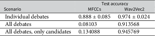
Table 3 shows the results from applying both MFCC-based and Wav2Vec2-based models for speech classification.Footnote 9 We devised three training scenarios: (1) classification based on individual debates, which involves differentiating between just two to three candidates per debate; (2) classification across all 156 distinct speakers; and (3) classification of only candidates but across all debates, which implies identifying among 34 candidate labels. The difference between the two models is significant and evident from the results. On individual debates, the Wav2Vec 2.0 audio embeddings model demonstrated a higher mean test accuracy of 0.974 (±0.024) across debates. The MFCC model still achieved a high value of 0.888 (±0.085) across debates, demonstrating its ability to perform well in simple classification tasks. More noticeably, when identifying among all speakers or only candidates, the Wav2Vec 2.0 model outperformed the MFCC model by a considerable margin, with test accuracies of 0.914 and 0.946, respectively, against the MFCC model’s 0.081 and 0.134, which expose its limitations when faced with many identities.
Accuracy on test data for the two models based on different features (MFCCs and Wav2Vec2) and different scenarios: (i) classification on individual debates (few speakers), showing average performance; (ii) classification on all debates (all 156 speakers); and (iii) classification on only candidates across all debates (34 speakers). The first scenario shows the average accuracy for all debates.

Table 3 Long description
The table consists of three columns: Scenario, M F C C s, and Wav2Vec2.
* Individual debates: M F C C s shows 0.888 plus or minus 0.085. Wav2Vec2 shows 0.974 plus or minus 0.024.
* All debates: M F C C s shows 0.08103. Wav2Vec2 shows 0.913568.
* All debates, only candidates: M F C C s shows 0.134088. Wav2Vec2 shows 0.945769.
The data indicates that Wav2Vec2 consistently outperforms M F C C s across all tested scenarios, particularly in the ‘All debates’ and ‘All debates, only candidates’ categories where M F C C s accuracy drops significantly.
Abbreviation: MFCC, Mel-frequency cepstral coefficient.
4.4 Emotional Classification with Audio Embeddings
The emotional tones of speech often reveal underlying sentiments, personal traits, and strategic communication choices. Political scientists have recently used tools like natural language processing and sentiment analysis due to their wider accessibility to understand these nuances. However, conventional textual analyses disregard acoustic cues present in the speaker’s voice.
Building from the previous applications, we explore the use of fine-tuned models for more complex classifications tasks, such as emotion recognition. Wav2Vec 2.0 embeddings already contain sufficient information to perform speaker identification without much fine-tuning for the specific task. Moreover, researchers have fine-tuned these audio embeddings to perform well in a variety of more complex tasks, from ASR to emotion recognition, and significant efforts have been dedicated to overcoming scarcity of training data for audio and generalizability in out-of-domain applications (Hsu et al. Reference Hsu, Sriram, Baevski, Likhomanenko, Xu, Pratap, Kahn, Lee, Collobert, Synnaeve and Auli2021).
Here, we use two models that aim to classify discrete basic emotions and their underlying dimensions. The first one, developed by SpeechBrain (Ravanelli et al. Reference Ravanelli2021), uses fine-tuned Wav2Vec 2.0 embeddings trained on the Interactive Emotional Dyadic Motion Capture (IEMOCAP) dataset by the University of South Carolina (Busso et al. Reference Busso2008). This is one of the oldest and widely used datasets containing approximately 12 h of visual, auditory, textual, and motion capture data of different actors in improvised and scripted scenarios showcasing different emotions. The model has an average reported test accuracy of 75.3% when recognizing four basic emotions: anger, happiness, sadness, and neutral.
The second model is a dimensional speech recognition model developed by Wagner et al. (Reference Wagner2023). They demonstrate that, by fine-tuning audio embeddings like Wav2Vec 2.0, the model can learn linguistic features (e.g., words associated with different positive and negative valence) to predict valence with a higher correlation than before. We can therefore expand the notion of sentiment analysis to valence, to consider not only what is said, but also how it is said. They present a very comprehensive performance comparison of several emotional dimension recognition models regarding their correctness (accuracy), robustness to noise, and fairness with respect to different speakers and biological sex. In particular, their models predict the dimensions of arousal, dominance, and valence. Arousal is defined as the intensity or energy level of an emotion (going from calm or relaxed to excited), dominance is the degree of assertiveness, control, and confidence conveyed in a speaker’s voice given an emotional state, and valence is the positivity or negativity of an emotion. It is combinations of these measures that generally define discretely labeled emotions.Footnote 10 The authors report state-of-the-art performances measured by concordance correlation coefficients (CCCs)Footnote 11 of 0.744 for arousal, 0.655 for dominance, and 0.638 for valence, in the MSP-Podcast datasetFootnote 12 (Lotfian and Busso Reference Lotfian and Busso2019), with good generalization to unseen datasets like IEMOCAP or MOSI (Multimodal Opinion-level Sentiment Intensity). The authors also report a very high robustness to noisy audio and no strong biases with respect to individual speakers or genders.
For political scientists working with these data, we emphasize that these definitions can vary across individuals, circumstances, or cultural contexts. Our aim here is to encourage and facilitate further research that will identify where cautious inferences are warranted. Following the example set by Rittmann (Reference Rittmann2024), it will be important for emotion and speech classification in political analysis to exhaust all possible avenues for comparative work, particularly in cultures outside the United States where female representation in debate is more common and rhetorical appeal and incentives differ. Many of the breakthroughs in understanding political deliberation have come from analyzing deliberation of minority groups, movements, and localized political discussion (e.g., Mansbridge Reference Mansbridge1983). With the growing availability of audio-transcription tools, computational analysis of political speech at scale is now feasible. Our aim is to help open this domain in a way that is both methodologically rigorous and attentive to its interpretive limits.
Measuring emotional dimensions with computational methods at a large scale opens a stream of possibilities for scaling existing research in political psychology and communication beyond textual information. As the emotional dimension of valence measures the positivity or negativity of an emotion, we can generalize the notion of sentiment by considering not only the textual contents of the speech but also the emotional cues hidden in the utterance. In the past, speech recognition models suffered from low performance on the valence dimension due to inability to encode the textual contents of the speech.Footnote 13
In Figure 4, we present the results derived from applying these models to presidential debates. Figure 4a illustrates the percentage distribution of the four discrete emotions (angry, happy, neutral, and sad) across each debate. A significant portion of utterances in most debates are classified as angry, whereas the majority of the remaining utterances are identified as neutral. There are few utterances labeled as sad, and only a few as happy—though the latter seems to have increased slightly in recent years. These classifications illustrate the prevalent serious tone in political debates. They also may reveal how disagreements between candidates that the presidential debate format constitutes by design result in many heated interventions classified as angry. Further research needs to investigate whether viewers also perceive these interventions as angry or neutral in comparison. Figure 4b identifies the candidates with the highest and lowest percentage of angry labels. It is interesting to note that candidates like Hillary Clinton and Jack Kemp, who appear among those with the highest voice pitch in Figure 3, are identified as more aggressive in their speaking style. Conversely, candidates such as Dick Cheney and Joe Lieberman, with some of the lowest voice pitches, appear calmer and less aggressive. In expert analyses of the first Trump–Clinton debate of 2016, Trump was found to use anger/threatening tone in 82.6% of his interventions, compared with Clinton’s 35.3% (Bucy et al. Reference Bucy2020). However, Trump does not appear as one of the candidates with the highest displays of anger in his voice. These contradictions require investigating their reflection in public perceptions to understand whether model misclassifications confuse stern debate or what political scientists and voters might consider good political deliberation, with aggressive speech.
Emotional analysis using fine-tuned Wav2Vec 2.0 models on the U.S. presidential debates. (a) Percentage of discrete emotional labels (angry, happy, neutral, and sad) in each of the debates. (b) Top five and bottom five candidates ranked by their percentage of utterance classified as angry in their speeches. (c) Top five and bottom five candidates rated by their average dominance, arousal and valence. (d) Normalized co-occurrence matrices comparing audio-predicted emotions (rows) with text-based emotional classifications (left) and sentiment labels (right).

Figure 4 Long description
Panel a is a stacked bar chart showing the percentage of emotional labels across 47 debates from 1960 to 2020. The y-axis represents percentage from 0 to 100. The x-axis lists debates chronologically. Legend indicates purple for ang, blue for hap, green for neu, and yellow for sad. Neutral and angry labels dominate most bars.
Panel b is a horizontal bar chart ranking candidates by percentage of ang labels. The top five are Anderson, H Clinton, Kemp, Kaine, and Stockdale, all above 70 percent. The bottom five are Ferraro, Dole, Lieberman, Carter, and Cheney, all below 20 percent.
Panel c contains three bar graphs for Dominance, Arousal, and Valence. Each shows the top five candidates in pink and bottom five in teal with error bars. For Dominance, H Clinton is highest and Cheney is lowest. For Arousal, H Clinton is highest and Cheney is lowest. For Valence, Gore is highest and Kemp is lowest.
Panel d features two normalized co-occurrence matrices. The y-axis for both is Audio emotion with rows for ang, hap, neu, and sad. The left heatmap compares this to Text emotion with columns for anger, disgust, fear, joy, neutral, sadness, and surprise. A strong vertical band shows high co-occurrence with neutral text across all audio emotions, ranging from 64 to 75 percent. The right heatmap compares Audio emotion to Text sentiment with columns for Negative, Neutral, and Positive. The highest co-occurrence is between all audio emotions and neutral text sentiment, peaking at 63 percent for hap.
Part of the discrepancy might stem from this four-label categorization being overly simplistic, failing to capture the full spectrum of nuances in political communication. Hence, in Figure 4c, we showcase results using the dominance–valence–arousal framework. Familiar names emerge in the high dominance–high arousal category: Hillary Clinton, Ross Perot, and John Anderson exhibit the highest average dominance and arousal, whereas Joe Lieberman and Dick Cheney have the lowest. Such findings suggest that Clinton, Perot, and Anderson display the most dominant speaking styles coupled with high arousal levels—potentially explaining why their utterances are often labeled as “angry.” This might also hint at a broader narrative suggesting female politicians often modulate their speaking style to appear more assertive (Jones Reference Jones2016). However, emotion recognition models are not neutral classifiers; they can encode and amplify biases related to gender, ethnicity, and vocal characteristics such as pitch and intonation. This may lead to systematic misclassifications, where female politicians are disproportionately labeled as “angry” or “emotional” even when using neutral or assertive tones—an issue that some of our findings already hint at. To prevent these distortions, model outputs must be critically validated against human-coded emotional interpretations to ensure fairer and more accurate assessments.
In contrast, figures like Dick Cheney and Joe Lieberman, who are linked with fewer angry statements, also rank lowest in the dominance–arousal matrix, denoting a calm and measured speaking style. None of the candidates, however, seems to stand out as having a particularly high or low valence in their speech, meaning that they do not showcase overwhelmingly positive or negative valence. It would be interesting to analyze how valence changes over time during a debate to identify moments of tension. Thanks to our first application where we synchronized text and audio, we could potentially study which topics of debate increase or decrease the valence (or sentiment) of the debate, opening up very interesting avenues of research using multimodal data. We caution strongly, however, against naïve interpretations, especially on cross-speaker comparisons. We have already discussed how variations in recording technology, postprocessing algorithms, or digital formats can influence how these features are processed by models, and to that we must add potential gender and racial biases that have emerged now. While these models might classify Clinton as aggressive or Cheney as nonaggressive, it is not easy to assert from the outputs of the model whether Clinton was truly expressing anger at a higher rate, or her neutral speaking style is closer to what the model considers “angry,” resulting in a higher false-positive rate. For this reason, we emphasize the need for speaker-dependent validation (through, e.g., human annotations of a subsample) or purely comparing within-speaker shifts with normalized outputs, akin to Figure 3d. We cannot emphasize enough that our contribution aims to open up doors for future analysis to understand whether these methods represent political speech and cognition well, and work consistently across language and gender differences (allowing studies of where and why they lose accuracy and introduce bias).
While these computational approaches offer the ability to analyze large-scale emotional patterns in political speech, they should be seen as starting points, not definitive measures of emotion. Figure 4d shows the level of agreement between two text-based classifiers (for emotions, bottom left; and sentiment, bottom right). This figure shows that a text-based emotion recognition model tends to classify most of the utterances as neutral, whereas the audio classifier shows more nuance (left). A coarser classifier based on sentiment (right) shows more correlations with audio-based emotions, such as correlating anger with more negative sentiment (32%), although it also shows co-occurrence of sadness with both positive and negative sentiment.
Emotion is more than simply a feature to be extracted—it is socially and politically constructed, shaped by context, audience expectations, and cultural norms. To truly grasp the role of emotional appeals in political debates, we need more than just algorithms. Mixed-methods approaches that integrate computational or quantitative analyses with qualitative methods are essential. These approaches do not just validate machine-learning outputs but uncover the “why” behind emotional expression in political and other contexts. We must not risk flattening the complexity of human communication by relying on mere numbers—turning it into data points, rather than acknowledging its dynamic and persuasive force.
5 Conclusion
Analyzing audio at scale offers a timely methodological response to developments like the deliberative turn in democratic theory, renewed interest in delivery of elite cues, the importance of emotion or pathos of populist speech, and how the affordances of new media affect public opinion. In political communication, vocal intonation and pitch can reveal how politicians convey sincerity, authority, or emotion, influencing voter reactions and campaign effectiveness (Nagel, Maurer, and Reinemann Reference Nagel, Maurer and Reinemann2012). Political psychology highlights the impact of emotional appeals (anger, fear, enthusiasm, and pride) on public opinion and voter behavior (Ridout and Searles Reference Ridout and Searles2011), whereas studies of party rhetoric show how emotional language supports populist mobilization (Widmann Reference Widmann2021). Extending such analyses beyond text to include other modalities, especially audio, promises a more nuanced view. Although emotional content of images (Iyer et al. Reference Iyer, Webster, Hornsey and Vanman2014) and facial/body expressions (D’Errico, Poggi, and Vincze Reference D’Errico, Poggi and Vincze2012) have also been studied in political communication, audio remains comparatively understudied and offers a rich, scalable domain for computational analysis, as demonstrated in this paper.
In conclusion, this paper has introduced a range of methods for analyzing political communication through audio data, including forced alignment for transcript synchronization, LLDs like pitch and energy, and machine learning models for speaker and emotion classification. While many of these approaches rely on statistical properties of audio signals rather than linguistic content, and can therefore be adapted across languages, their implementation, especially for those based on machine learning, might require language-specific resources or training data. As such, caution is needed when applying them beyond their original context. We also emphasize that these models remain under development and must be used critically: biases affecting gender and other minority groups can distort results and must be recognized and addressed. A simultaneously technical and theory-informed approach that is reflexive and context-aware is essential to ensure these tools support, rather than obscure, the complexities of political discourse.
Supplementary Material
For supplementary material accompanying this paper, please visit https://doi.org/10.1017/pan.2025.10031.
Data Availability Statement
Replication code for this article has been published in the Political Analysis Harvard Dataverse at https://doi.org/10.7910/DVN/K3I16E (Mestre and Ryan Reference Mestre and Ryan2025) and GitHub: https://github.com/rafamestre/audio-as-data.
Funding Statement
The authors would like to thank UK Research and Innovation funding (Grant Nos. MR/S032711/1 and MR/Y02009X/1).
Competing Interest
The authors declare no competing interests.


 Open access