2. EXISTING APPROACHES

A number of different approaches exist to distinguish between whether the received satellite signals have travelled in direct path down to the antenna (satellites in LOS), or have reflected off the facades of the surrounding buildings (NLOS):

• • At the hardware level, one can detect and eliminate signals arriving from below the antenna. It is generally assumed that reflected signals rising up to the antenna from the ground surface or from the roof of the vehicle itself are efficiently attenuated by its ground plane and its designed sensitivity pattern. Moreover, direct signals have right-handed circular polarization whereas many reflected signals have left-handed polarization. Also reflected signals are typically weaker. In general, signals with left-handed polarization and those with low strength are dismissed by antenna and receiver design respectively. This is done in most GNSS equipment, but with limited success, and always within the limitation imposed by an adequate balance in terms of required sensitivity.

• • Other hardware approaches consist of mounting an additional sensor, when this is possible on board, for example an infrared (Meguro et al., Reference Meguro, Murata, Takiguchi, Amano and Hashizume2009) or fish-eye (Marais et al., Reference Marais, Ambellouis, Flancquart, Lefebvre, Meurie and Ruichek2012) camera to directly measure building boundaries by image processing.

• • At the navigation software level, consistency checking of the solution computed, for instance by conventional least squares, similar to Receiver Autonomous Integrity Monitoring (RAIM) is used (Jiang et al., Reference Jiang, Groves, Ochieng, Feng, Milner and Mattos2011). However, should too many observations be affected, such an approach fails. Spatial constraints applied to positioning solutions can also help, these being extracted from a database such as road plane geometry for vehicles (Peyraud et al., Reference Peyraud, Bétaille, Renault, Ortiz, Mougel, Meizel and Peyret2013), or numerical terrain model data for land navigation in general (Jiang and Groves, Reference Jiang and Groves2012; Groves and Jiang, Reference Groves and Jiang2013), which fuses consistency checking, height aiding and also signal strength. This assumes that the accuracy of these data is at least at the same level as the GNSS measurement, which is not always true.

• • Last, but not least, software approaches can also consider the use of geometric city models.

Improving GNSS positioning in urban canyons with Three-Dimensional (3D) maps has been addressed by a few research teams in the past few years: first Bradbury et al. (Reference Bradbury, Ziebart, Cross, Boulton and Read2007) and Suh and Shibasaki (Reference Suh and Shibasaki2007) in parallel, and for the most recent references: Wang et al. (Reference Wang, Groves and Ziebart2012), Obst et al. (Reference Obst, Bauer, Reisdorf and Wanielik2012) and Peyraud et al. (Reference Peyraud, Bétaille, Renault, Ortiz, Mougel, Meizel and Peyret2013). Whereas these articles present methods that do not model the additional path delay due to signal reflection, a few others, in contrast, will actually make this next step forward and include Bourdeau et al. (Reference Bourdeau, Sahmoudi and Tourneret2012), Miura et al. (Reference Miura, Hisaka and Kamijo2013), Bétaille et al. (Reference Bétaille, Peyret, Ortiz, Miquel and Fontenay2013a, Reference Bétaille, Peyret, Ortiz, Miquel and Fontenay2013b) and Suzuki and Kubo (Reference Suzuki and Kubo2013).

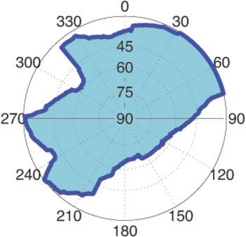
Thus Bradbury et al. (Reference Bradbury, Ziebart, Cross, Boulton and Read2007) and Suh and Shibasaki (Reference Suh and Shibasaki2007) could validate the various conditions of reception (i.e. LOS, diffraction and reflection) that were predicted by ray-tracing in a 3D city model, carrying out real world experiments. Following this approach, Wang et al. (Reference Wang, Groves and Ziebart2012) figure out the satellite visibility problem using similar techniques and data. A building boundary is computed, i.e. a satellite visibility domain, represented in the usual polar diagram also called a “sky plot” (Figure 1), for any possible rover location in a grid. This building boundary makes possible LOS/NLOS separation.

Figure 1.

Sky plot of building boundaries from the perspective of GNSS users (Wang et al., Reference Wang, Groves and Ziebart2012).

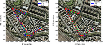
Obst et al. (Reference Obst, Bauer, Reisdorf and Wanielik2012) have a similar approach, with some probabilistic aspects to cope with the uncertainty of both the model and the rover location a priori. This very last point (i.e. the question where to initialise and generate the geometrical computation) is actually the trickiest. First, the domain where the solution may lie can generally be constrained, in particular as concerns vehicle mobility: Jiang and Groves (Reference Jiang and Groves2012) uses height aiding; Peyraud et al. (Reference Peyraud, Bétaille, Renault, Ortiz, Mougel, Meizel and Peyret2013) applies road plane constraints. In Peyraud et al. (Reference Peyraud, Bétaille, Renault, Ortiz, Mougel, Meizel and Peyret2013) no ray-tracing is done, but a virtual image is generated in the azimuth of each satellite, from which a simple geometrical process determines the corresponding critical elevation: authors have demonstrated the interest of selecting only the satellites above critical elevations. They proved the advantage of the LOS/NLOS selection versus the SNR-based (Signal-to-Noise Ratio, 3D model-free), in particular on a final position using the road constraints (Figure 2). In Groves and Jiang (Reference Groves and Jiang2013), in addition to geometrical constraints, SNR and consistency checking (i.e. RAIM derived) have been analysed in multiple criteria combinations.

Figure 2.

Overview of the solutions obtained with (LOS/NLOS or SNR) strategies without (a) and with (b) application of road constraint (Peyraud et al., Reference Peyraud, Bétaille, Renault, Ortiz, Mougel, Meizel and Peyret2013).

In addition, knowledge of the local building geometry makes possible the estimation of the additional path travelled due to reflection, which is an unbounded positive delay in the case of NLOS. This estimation, like LOS/NLOS selection, is also particularly dependent on the assumed position of the rover.

An exploration of the solution domain has been conducted in Miura et al. (Reference Miura, Hisaka and Kamijo2013). The best consistency between the assumed solution and that finally obtained from grid points ray tracing and NLOS selection and correction was sought. Bétaille et al. (Reference Bétaille, Peyret, Ortiz, Miquel and Fontenay2013b) proved that such consistency checking could give good results too, with the simplified street model introduced in Bétaille et al. (Reference Bétaille, Peyret, Ortiz, Miquel and Fontenay2013a): the idea was to test multiple lateral candidate positions across the street. Similarly, Suzuki and Kubo (Reference Suzuki and Kubo2013) used particle filtering to explore the solution domain.

Bourdeau et al. (Reference Bourdeau, Sahmoudi and Tourneret2012) show how the local building geometry can help in code tracking, which goes beyond the Position-Velocity-Time (PVT) computation stage in the receiver, and tackles the signal processing stage itself.

In addition to this LOS/NLOS discrimination concept, another idea (shadow matching) takes advantage of the possibility of predicting which satellites will be visible from the rover's point of view, and compares this prediction to the actual observation (Groves, Reference Groves2011), and more recently in Wang et al. (Reference Wang, Groves and Ziebart2013) and Yozevitch et al. (Reference Yozevitch, Ben-Moshe and Dvir2014). One can restrict the user's location domain by considering those satellites present in the ephemeris and for which no measurement is made. For illustration purposes, let us assume that the unique signal source considered is the Sun, this concept looks like the intuitive determination one can make of which side of a street is travelled at a given time just considering whether or not the position is in the shade or in sunlight. The same principle is used in this paper: for each GNSS satellite feasibly available in the current ephemeris file, the grid of its signal availability is determined from the city model data thus constraining what positions are realistic given the signals tracked.

These applications often seek to improve the rover position sufficiently to discriminate between different sides of a road, or between traffic lanes. Hence, they require 3D city models with geometric accuracy at the sub-metre level.

A major real-time processing problem of 3D models is due to their size and access time through embedded Geographical Information Systems (GISs). In the research work related here, urban canyons have been modelled in a very simple manner, with width and height parameters as in Bétaille et al. (Reference Bétaille, Peyret, Ortiz, Miquel and Fontenay2013a) but allowing for asymmetry between both sides of streets. The key point of the model produced is its simplicity, to the extent that it matches the polyline format of most digital road maps. The approximations made by this modelling have been validated in term of final positioning accuracy. The article will first develop the model (Section 3), second explain how it has been automatically computed from a public national data base available in France (Section 4), and third prove its efficacy in positioning improvement with full-scale test cases (Section 5). Last, but not least, the trade-off between the simplicity in 3D modelling, with its corresponding data storage optimality and real-time usability on the one hand, and the positioning accuracy obtained using such a model on the other hand, will be discussed, comparing our approach to the state-of-the-art (Section 6), before concluding (Section 7).

3. THE URBAN TRENCH MODEL

For the initial proof of concept already published (Bétaille et al., Reference Bétaille, Peyret, Ortiz, Miquel and Fontenay2013a), streets were considered as parallelepipeds, so called “urban trenches”, from which LOS/NLOS satellite signal discrimination was made possible. The method consists of four phases:

• • Characterisation of the 3D environment;

• • Detection of the NLOS satellite signals;

• • Correction of the additional path in their measurements;

• • Computation of the positioning solution.

We made the choice intentionally to call our model of urban streets “urban trench” and not “urban canyon” to clearly differentiate the two concepts. “Urban canyon” is indeed often used in the literature to depict a situation when high buildings are surrounding the receiver, creating propagation problems. “Urban trench” depicts a simplified model of any street, considering that the rows of buildings can be approximated by an average geometry. Any kind of street can be modelled by the “urban trench” model, even those with low buildings that are far from being “urban canyons”.

3.1. The characterisation of the 3D environment

Only street sections with “homogeneous geometry” are concerned (see Figures 3 and 4), while elsewhere a conventional positioning algorithm will operate. Criteria defining these sections correspond to considering streets as parallelepipeds, i.e.:

• • A constant street direction;

• • The same width (W) of the street all along the section;

• • The same height (H) of building all along the section, and on both sides;

• • A unique lateral position (P) occupied by the vehicle in this section, i.e. no lane change: this is measured from left to right, in percentage of the total width from side to side, and with the direction of the street duly defined.

Figure 3.

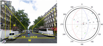
Urban trench and (W, H, P) parameters along a boulevard in Paris (Bétaille et al, Reference Bétaille, Peyret, Ortiz, Miquel and Fontenay2013b), and an example of a “mask of visibility” with W = 30 m, H = 15 m, and P = 0·65.

Figure 4.

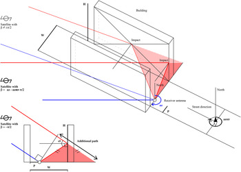
Urban trench geometry with W, H and P parameters and 2 NLOS satellites (one with an azimuth orthogonal to the street direction, i.e. β = −π/2); β denotes the angle difference between the satellite azimuth and the street direction, this being arbitrarily set in the data base, irrespective of the driving direction.

Several test campaigns were performed, with data collected in Nantes, Paris and Toulouse. The VERT (Véhicule d'Essais et de Reference Trajectographique, the Ifsttar Geoloc lab test vehicle) provided a decimetre-accurate GPS time-stamped reference trajectory (Ortiz et al., Reference Ortiz, Peyret, Renaudin and Bétaille2013), even in the deepest urban canyons of these city centres, by means of its embedded instruments: a LandINS from IXSEA coupling an inertial measurement unit with post-processed kinematic solutions from a Novatel dual-frequency DLV3 GNSS receiver and permanent network data. The receiver used in the test was the automotive and high-sensitivity GPS Ublox LEA6-T, 5 Hz, mounted on the roof of the vehicle.

Throughout the test areas in Nantes, Paris and Toulouse, width and height have been estimated from Google Earth views. Horizontal distances were measured manually with the rule available in Google tools, whilst total floor numbers, visible from Street View gave an approximation of vertical distances, considering floor heights of 2·5 or 3 m depending on the construction architecture.

The position of the vehicle in the across-street direction was approximated (Table 1), taking into account the number of lanes, including cycling lanes and pedestrian avenues at road section centres (in addition to sidewalks), which are common in large boulevards.

Table 1.

Street configurations and lateral position values.

The principle here is to model the characteristics of the urban trench, where feasible, using a parameter triplet (W, H, P), which is used in the subsequent modelling and estimation scheme. This is illustrated in Figure 3.

3.3. The correction of additional path length

In case of one or several reflections and no interference with the direct signal, part of the measured pseudo-range is directly due to the additional path travelled by the signal. Geometrical considerations are again used to compute this error, as shown in Figure 4 in the case of a unique reflection. The critical elevations and additional distances corresponding to 1, 2 and 3 reflections are given in Table 2.

Table 2.

Critical elevations and additional distances for satellites situated on the left side of the street, i.e. (−π < β < 0) or (π < β < 2π).

Note: for satellites situated on the right side, i.e. (−2π < β < −π) or (0 < β < π), just replace P by 1-P.

4. AUTOMATIC CHARACTERISATION BY URBAN TRENCHES AND ADAPTATION OF THE NLOS DETECTION AND CORRECTION

The aim of this automatic characterisation is to determine width and height attributes of polylines, i.e. those arc segments representing the streets in position (and direction). That way, the complete geometry of urban trenches will be obtained. First we will make the hypothesis that our vehicle runs on the nearest map-matched arc segment.

To approximate the urban trench model, we use the database called BD Topo ® produced by the French Institute of Geographic and Forest Information (IGN):

• • The distances on the left and the right to the closest building;

• • The heights on the left and the right of the buildings along the street.

The final data item to determine is the direction of the arc segment. All these values were computed with an algorithm working with the open-source software: PostgreSQL and its extension: PostGIS (http://postgis.net/docs). Simple SQL requests have been programmed. Sections 4·1 to 4·4 will completely explain the process. It includes a map-matching step, for which we could not use the a priori least squares solutions because of their inaccuracy. Instead, the reference trajectory has been used so far.

The output of the characterisation process is a simple table giving width on the left, width on the right, height on the left, height on the right and the street direction at every epoch during the tests performed.

4.2. Algorithm for urban trench modelling

The aim is to extract the values described in the previous paragraph, namely the distances from each arc to the left and right buildings, and their respective heights. We must therefore know the arc direction to determine unambiguously the left and right sides of a trench. We produce, for each arc of the BD Topo ®, a table (id, W1, W2, H1, H2, direction). For this we will use the PostGIS spatial database.

The shapefiles of the BD Topo ®, specifically road and building layers, are used. A selection box in Quantum GIS (a freeware software package) enables us to specify a zone windowing the experiment area. The corresponding data from the layers will be processed using PostgreSQL through the shp2pgsql PostGIS tool.

4.2.1. Determination of widths

Measuring the distance from an arc to a building uses the ST_Distance PostGIS function that returns the minimum distance between two geometric objects, whether they are of the same type (point, line, surface) or not. As a first step, it is therefore necessary to identify buildings lining the street (left or right). For this we will use a buffer area.

The buffer takes a geometric object (e.g. a line or an arc) and a distance given by the user. In our case, we will use a half-buffer: this is a buffer area from only one side of the source geometric object.

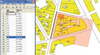
Taking a half-buffer extended from the arc of the road layer, and a large enough input distance parameter, we will be able to identify buildings contained or intersected in this area through ST_Intersects function (Figure 5). The identifiers of each detected building will then be stored in a temporary table as well as their distance from the arc that is to be characterised as an urban trench.

Figure 5.

Half-buffer (100 m wide, see Section 4.3) used for the determination of side width; the arc under consideration is underlined.

The minimum distance in the temporary table finally fills in the width parameter for left and right sides successively, and for every arc contained in the zone.

4.2.2. Determination of heights

The building layer of the BD Topo ® database contains the height of each building. The distance between the arc studied and the nearest building on each side is also known, so we will again use a half-buffer to identify the buildings lining the street. However, the search width used will correspond to the width of side already calculated in the previous step to which we add a few metres to consider only the closest buildings to the street.

Once again we use the ST_Intersects function and store the identifier of the building and its height in a temporary table. Finally, we calculate the average height using the avg PostgreSQL function for each side of the arc, which fills in the height parameter for left and right sides. This is repeated for every arc in the zone.

4.2.3. Determination of the arc direction

The last data to extract from the map database, the direction of each arc, is essential in the following calculation of the rover position since it indicates the direction of the arc and sets the left and right sides. The ST_Azimuth function is used, which returns the heading between two given points, these being returned by the ST_StartPoint and ST_EndPoint functions applied to the arc concerned (in PostGIS 2).

4.6. Artefacts

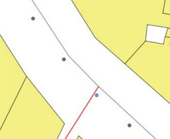
The simple map-matching algorithm used does not take into account certain parameters (such as direction). Some points may mismatch. Typically, in Figure 6, the point near the crossroad will be associated with the arc perpendicular to the route, so it will not be assigned the correct parameters of urban trench. Quddus et al. (Reference Quddus, Ochieng and Noland2007) reviews more sophisticated algorithms where this problem is fixed.

Figure 6.

Perturbation of the simple map-matching algorithm used.

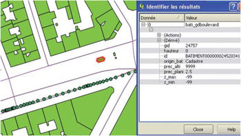
There are also artefacts related to the BD Topo ® building layer. In some areas there are “buildings” that would be more regarded as street furniture. Their height is zero (since they were borrowed directly from a map source that does not specify geometry but instead cadastre information). In Figure 7, the selected item (a kiosk) is in the middle of the street, and the reference trajectory appears in a series of points. The arc map-matched will not have correct urban trench attributes because on one side buildings are properly identified, but on the other, the width will be too low and of zero height because of the presence of this booth. It was therefore decided to remove from the building layer all the elements whose height is zero before retrieving urban trench data.

Figure 7.

A kiosk (of null height) that perturbs the urban trench determination.

Last, the BD Topo ® road layer also includes bridges, which are shown as “crossing” arcs that actually do not intersect. These linear features are poorly characterised. The search for the nearest building returns null, so we consider that the visibility extends to the whole sky. Locally, we will not expect any improvement in the calculation of the vehicle position in these configurations.

5. THE TEST CASES AND POSITIONING IMPROVEMENT

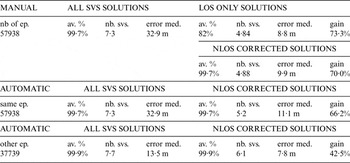
First tests were performed in Nantes for feasibility purposes, in the area known as Ile de Nantes, for 20 minutes, from which 5 minutes were included in urban trenches. Then in Paris, XIIth district, 2 h½ (40 minutes in urban trenches) and Haussmann Grands Boulevards, 5 h½ (3 h¼ in urban trenches), and in the business centre of La Défense (1 h and 20 minutes). In the latter, it was not possible to define properly any urban trench, except (10 minutes) along the Avenue Charles de Gaulle in Neuilly, which is quite similar to a grand boulevard. Lastly, a test case of 50 minutes was carried out in the city centre of Toulouse (20 minutes in urban trenches), with a building architecture very different from Paris and Nantes. All these tests were done in 2012. Tables 3a to 3e gives the results obtained in the different test cases:

• • “nb of ep” is the number of epochs under consideration (5 Hz receiver data);

• • “av. %” is the availability, i.e. the fraction of the number of epochs, in %, when a solution could be computed by conventional least squares;

• • “nb svs” is the average number of satellites used in the computed solutions;

• • “error med” is the 3D median error in position;

• • “gain” is the relative decrease of the 3D median error obtained using the urban trench approach with respect to that obtained using all satellites.

Table 3a.

3D median error and gain achieved in Nantes for the different test cases.

Table 3b.

3D median error and gain achieved in XIIth district for the different test cases.

Table 3c.

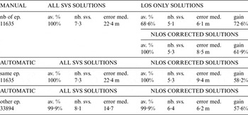
3D median error and gain achieved in Grands Boulevards for the different test cases.

Table 3d.

3D median error and gain achieved in La Défense for the different test cases.

Table 3e.

3D median error and gain achieved in Toulouse for the different test cases.

The purpose was not only to validate the automatic model with respect to the manual one (which is indeed feasible where urban trenches have been manually determined), but also to measure the impact of the new modelling anywhere else, because the last model is actually available all over France.

For each zone, the statistics considered are the average number of satellites used in the solution, and the 3D median error (this, contrary to the mean error, is not affected by possible outliers). The error is defined as the difference between the computed solution and the reference trajectory at the same epoch.

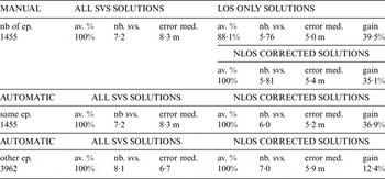
The different test cases are respectively:

• • Epochs where urban trenches were constructed by the manual model

  • – solution (always by least squares) using all satellites

  • – solution using LOS satellites only, which decreases the availability

  • – mixed solution using LOS and NLOS satellites, with corrected ranges

• • The same epochs as with the manual model, but using the automatically generated trench models

  • – solution using all satellites

  • – mixed solution using LOS and NLOS satellites, with corrected ranges

• • On all other epochs where the automatic model works but not the manual one

  • – solution using all satellites

  • – mixed solution using LOS and NLOS satellites, with corrected ranges.

The improvement is always given with respect to the basic navigation solution using all satellites.

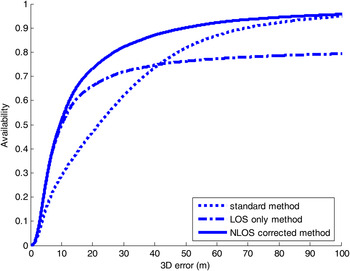
Note that only LOS statistics have not been added in Tables 3 for the automatic model, but they are almost similar to those for the manual model. They are nevertheless aggregated and displayed in Figure 8.

Figure 8.

Cumulative distribution function of the absolute error in 3D, for standard and urban trench solutions, using the automatic 3D model, for all epochs and all test sites in Nantes, Paris and Toulouse (10 hours of data); note that the asymptote is lower when using LOS only, because solutions are often not computable, which can also be interpreted as an infinite error

Several conclusions arise: first of all, a gain (between 30% and 90%) is always achieved in urban trenches, despite various urban environments. It is slightly less (a few points less) when NLOS satellites are introduced in the least squares estimates (after range correction), but the improvement this strategy brings in terms of availability makes it valuable anyway. Actually, where the availability was reduced by 10% to 30%, almost full availability is recovered. The second conclusion concerns the automatic versus manual modelling: the gains are not significantly different. Last, but not least, a gain (between 10% and 60%) is also achieved where the automatic model is applied, which would not be achieved when the manual model is supplied. These conclusions justify the effort of studying the problem of LOS satellites selection along with NLOS ranges correction (when necessary to get epoch per epoch least squares solutions).

Figure 8 aggregates all epochs and all test sites (i.e. 10 hours of data), irrespective of whether or not they belong to the former manually modelled urban trenches. The cumulative 3D error distribution is displayed, for the standard estimator, for the estimator using LOS satellites only, and for the estimator mixing LOS and NLOS satellites, applying the new automatically modelled urban trenches.

Whereas only 4½ hours were modelled manually, here the BD Topo ® database was used automatically everywhere, which led to a near 10 hour final data set. The LOS only method availability is around 80%, while the standard and NLOS corrected methods reach almost 100% (La Défense showing the trickiest environment: this is Paris business centre, where tall buildings behind smaller ones have probably not been included in the 5 metres parameter used for the automatic determination of heights, see Section 4.3). The median error in 3D has been reduced from 21·7 m down to 9·4 m, i.e. 56% improvement globally.

6. TRADE-OFF BETWEEN MODEL SIMPLICITY AND POSITIONING IMPROVEMENT

Both the manual and automatic building models are obviously very crude compared to the approaches used by other research groups working on 3D-model-aided GNSS. Let us just mention that actually:

• • the accuracy of the geometric objects in BD Topo ® is one order of magnitude below that of other databases, e.g. in France: BATI 3D ®, used by (Peyraud et al., Reference Peyraud, Bétaille, Renault, Ortiz, Mougel, Meizel and Peyret2013), i.e. the metre versus the decimetre; note however that BATI 3D ® covers only very few cities, like Paris XIIth district;

• • moreover, in our approach the geometry is averaged per road arc, which penalises this approach where the buildings vary in height and/or if there are gaps between them so they do not make continuous facades;

• • another drawback is due to the assumption that the urban trenches are infinite in length: at a road junction, consequently, the geometry of the street one comes from will be used until the junction centre – unless specific road arcs exist in the junction itself – despite such an area offering a relatively open sky in general. The most advanced state-of-the-art approaches already mentioned in Section 2 consider that the building geometry is specific in each satellite azimuth, whereas our approach regards urban trenches as infinite;

• • no grid of possible rover positions or exploration of the solution domain is used here, but one assumes that the closest road arc is occupied to feed the building boundaries determination process.

Even if in practice the urban trench model can be computed everywhere, it will actually apply optimally only where the building geometry is regular and simple enough. For example, a grid of building boundaries (Figure 1) could provide a much better positioning performance in more singular and complex environments.

The objective in Section 6 is to measure the performance penalty in terms of positioning accuracy compared to a sophisticated model, and determine the benefit in counterpart in terms of computing performances.

In a preliminary proof of concept made in our group of research (Peyret et al., Reference Peyret, Bétaille and Mougel2011), the same BD Topo ® source database was used directly and the LOS/NLOS separation, i.e. the computation of the critical elevations, was based on the use of virtual images generated in the azimuth of the tracked satellites, an original process equivalent of ray tracing for that purpose. A comparison of the selection of satellites and final accuracy using those LOS only is possible, between this method and that using urban trenches.

A series of tests were done in Nantes, in 2011, in the same area as the 2012 tests already mentioned in Section 5. Ublox LEA4-T receiver data were logged at 4 Hz, for approximately 45 minutes in the morning and in the afternoon. Tables 4 display the confusion matrix between the two approaches for the selection of satellites.

Table 4a.

Confusion matrix (morning test).

Table 4b.

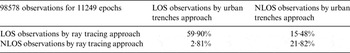
Confusion matrix (afternoon test).

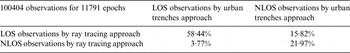
The urban trench approach obviously over-determines NLOS configurations in this data set, which confirms that its geometrical assumptions do not completely apply. In particular at intersections, the hypothesis that urban trenches are infinite in length causes false building boundaries in crossroad directions, where in fact open sky conditions apply.

In terms of positioning accuracy, the 3D median error using LOS satellites only grows from 9·0 m (using ray tracing) to 10·3 m (using urban trenches) in the morning, and from 10·8 m to 12·7 m in the afternoon, which is still below the accuracy of the solution using all satellites: 14·3 m and 15·2 m respectively. To conclude, the performance penalty of the urban trench modelling globally equals 16·7% for this data set (relative error growth).

On the one hand, there is an error growth, but on the other hand, much better computing performances have been achieved.

Using the previous example for computational efficiency is not straightforward. Let us simply quote that Peyraud et al., (Reference Peyraud, Bétaille, Renault, Ortiz, Mougel, Meizel and Peyret2013) – based on the same ray tracing approach – mentions “an off-line process in replay mode”: in other words, a very challenging real-time implementation. In terms of data storage, one can refer to Groves et al. (Reference Groves, Jiang, Wang and Ziebart2012), which states that “a 4 GB flash drive could store building boundary data for 2,500–25,000 km of road network, depending on compression”. This represents an interval between 0·16–1·6 MB/km. For Nantes centre, our model covers 188 km with less than 1 MB, i.e. 0·005 MB/km, near two orders of magnitude below, because we store a few urban trench parameters only per arc segment: Id, co-ordinates and direction, W1, W2, H1, H2 (actually we have just added two widths and two heights). So this makes the urban trench approach highly competitive for real-time implementation in navigation systems and embedded ITS applications.

7. CONCLUSIONS AND PERSPECTIVE

We managed to automate the creation of urban trenches from the BD Topo ® database using an approach independent of the reference trajectory of the rover. This is a major evolution compared to the initial manual modelling. To start the geometric calculation of multipath, the vehicle position is map-matched onto the nearest road arc segment (we actually do not use the reference trajectory except for determining surely by map-matching in which urban trench it is located). We can also say that this assumption is relevant since the results are consistent with those obtained initially with the manual model. It is feasible to apply the technique throughout France (entirely covered by the BD Topo ® database), with a successful applicability to streets that fit the simplified building boundaries.

We have several future problems to address:

• • The positioning a priori (before map-matching) could use a generic street geometry, and an SNR-based threshold; it is also very promising to run a filter (e.g. Kalman) instead of a least squares estimator, in order to predict this initial positioning;

• • The map-matching could be regarded as a multiple hypotheses problem, first, because multiple road segments should be considered where the position uncertainty is large, and second, because next generation maps will be certainly based on a multiple lanes road representation;

• • The positioning a posteriori (after satellite selection and range correction) should feed the map-matching process and consequently ensure a total independence of the complete process with respect to reference trajectory;

• • Instead of regarding urban trenches as infinite, the elevation mask could be characterised more finely, sampling azimuth from the rover point of view: a trade-off between computation through-put and modelling should be found. In the current research, 10 hours of data could be automatically processed, whereas only 4½ hours had been made manually, i.e. less than half obviously considered in urban trenches. A future outcome of our research would be the estimated proportion of streets where the urban trench method works best, despite its simplified building boundary representation. Its systematic application until the extremities of road arcs (i.e. even at junctions) should be reconsidered.