

1. INTRODUCTION
Air temperature (T air) is an important input for hydrological, ecological and climate models. Extensive studies related to recent global warming have demanded more representative air temperature observations, especially in high-elevation areas (Liu and Chen, Reference Liu and Chen2000; Qin and others, Reference Qin, Yang, Liang and Guo2009; Cai and others, Reference Cai, You, Fraedrich and Guan2017). Since the Tibetan Plateau (TP) is considered as one of the most sensitive areas in the world to climate change, it has attracted numerous modeling studies on hydrology and glacier changes (Caidong and Sorteberg, Reference Caidong and Sorteberg2010; Gao and others, Reference Gao, He, Ye and Pu2012; Zhang and others, Reference Zhang, Su, Yang, Hao and Tong2013; Lutz and others, Reference Lutz, Immerzeel, Shrestha and Bierkens2014; Gao and others, Reference Gao2015). However, the data-sparse problem of T air is a limitation in mountainous areas (Zhang and others, Reference Zhang, Zhang, Ye, Che and Zhang2016a), and can be worse for hydrological and glacier mass-balance modeling in glacierized regions such as the TP (Yang and others, Reference Yang2011; Gao and others, Reference Gao, He, Ye and Pu2012; Zhang and others, Reference Zhang, Hirabayashi and Liu2012, Reference Zhang2015). The well-known temperature lapse rate (TLR) with increasing elevation is commonly used for T air interpolation (Li and others, Reference Li2013a), especially in glacierized basins over the TP (Zhang and others, Reference Zhang, Su, Yang, Hao and Tong2013, Reference Zhang2015; Immerzeel and others, Reference Immerzeel, Petersen, Ragettli and Pellicciotti2014; Gao and others, Reference Gao2015). However, the TLR can vary both temporally and spatially (Minder and others, Reference Minder, Mote and Lundquist2010; Li and others, Reference Li2013a). In reality, the limited number of stations within or near a mountainous river basin may create large uncertainty in the representativeness and accuracy of the estimated TLR, mainly because most stations are located in valley and low-altitude areas (Zhang and others, Reference Zhang, Zhang, Ye, Che and Zhang2016a).
Land surface temperature (LST) is an important variable in the studies of land surface physical processes (Wan, Reference Wan2008; Li and others, Reference Li2013b; Wu and others, Reference Wu, Wang, He and Jiang2015). To alleviate the data-sparse problem, remotely sensed LST data have been widely used for T air estimation based on the strong correlation between LST and T air in mountainous areas around the world (Fu and others, Reference Fu2011; Benali and others, Reference Benali, Carvalho, Nunes, Carvalhais and Santos2012; Kilibarda and others, Reference Kilibarda2014; Kloog and others, Reference Kloog, Nordio, Coull and Schwartz2014; Good, Reference Good2015; Zhang and others, Reference Zhang, Zhang, Ye, Che and Zhang2016a). Compared with the limited station observations, the use of satellite LST data is an optimal option for adequately characterizing the temporal and spatial patterns of LST in broad regions (Li and others, Reference Li2013b). Owing to the middle spatial and temporal resolution, MODerate resolution Imaging Spectroradiometer (MODIS) LST products have been successfully used in various fields including surface radiation (Bisht and others, Reference Bisht, Venturini, Islam and Jiang2005; Wang and others, Reference Wang2005), evaporation (Tang and others, Reference Tang, Li and Tang2010), urban heating island (Imhoff and others, Reference Imhoff, Zhang, Wolfe and Bounoua2010; Pichierri and others, Reference Pichierri, Bonafoni and Biondi2012), climate change (Qin and others, Reference Qin, Yang, Liang and Guo2009; Cai and others, Reference Cai, You, Fraedrich and Guan2017), hydrological modeling (Wang and others, Reference Wang, Koike, Yang and Yeh2009; Zhou and others, Reference Zhou2015), lake surface temperature (Schneider and others, Reference Schneider2009; Zhang and others, Reference Zhang2014) and air temperature estimation (Benali and others, Reference Benali, Carvalho, Nunes, Carvalhais and Santos2012; Zhu and others, Reference Zhu, Lű and Jia2013; Zhang and others, Reference Zhang, Zhang, Ye, Che and Zhang2016a). MODIS LST products are generated using the generalized split-window algorithm developed by Wan and Dozier (Reference Wan and Dozier1996), with accuracies better than 1 K on homogeneous surfaces (Wan and others, Reference Wan, Zhang, Zhang and Li2002; Wan, Reference Wan2008). Careful validation and evaluation of remotely sensed LST data is the basis of efficient application (Bosilovich, Reference Bosilovich2006). Validation of MODIS LST over various vegetated land cover types such as grasslands, pastures, forests and croplands shows relatively low accuracies with root-mean-squared-differences (RMSDs) of 1–4 K owing to a lack of accurate observations of emissivity and pixel heterogeneity (Bosilovich, Reference Bosilovich2006; Wang and others, Reference Wang, Liang and Meyers2008; Wang and Liang, Reference Wang and Liang2009; Li and others, Reference Li2014; Krishnan and others, Reference Krishnan2015).
MODIS LST data used in cryosphere science are applied mainly for validation and evaluation in Greenland (Hall and others, Reference Hall2008a, Koenig and Hall, Reference Koenig and Hall2010), the Arctic (Langer and others, Reference Langer, Westermann and Boike2010; Westermann and others, Reference Westermann, Langer and Boike2011, Reference Westermann, Langer and Boike2012) and Antarctic areas (Hall and others, Reference Hall, Key, Casey, Riggs and Cavalieri2004; Scambos and others, Reference Scambos, Haran and Massom2006; Wang and others, Reference Wang, Wang and Zhao2013b; Meyer and others, Reference Meyer2016). The TP has an average elevation of 4000 m and extensive distribution of glaciers (Yao and others, Reference Yao2012). It is also referred to as ‘the Third Pole’ outside the Arctic and Antarctic regions (Qiu, Reference Qiu2008). The previous validation and accuracy evaluation studies of MODIS LST data in the TP are focused mainly on vegetated land cover (Wan and others, Reference Wan, Zhang, Zhang and Li2002; Yu and Ma, Reference Yu and Ma2011; Wang and Min, Reference Wang and Min2014; Min and others, Reference Min, Yueqing and Zhou2015). However, the performance of MODIS LST on glacier surfaces in the TP remains unknown because of the limited temperature measurements in glacierized areas.
In this study, we comprehensively evaluate the performance of MODIS LST for T air estimation in glacerized areas of the TP. MODIS LST data are firstly compared with ground measured LST at two glacier sites to evaluate the accuracies of MODIS LST on glacier surfaces. Both MODIS daytime and night-time LST data are further used for T air estimation. The estimated T air are evaluated with observed daily mean air temperature (T mean), minimum air temperature (T min) and maximum air temperature (T max) at each glacier site. TLR is commonly used for T air estimation in glacierized basins (Immerzeel and others, Reference Immerzeel, Petersen, Ragettli and Pellicciotti2014; Zhang and others, Reference Zhang2015). For further evaluation, performances of the T air estimation from MODIS LST are also compared with those using TLR.
2. DATA
2.1. Ground measurements
Surface temperatures of four glaciers (Parlung Zangbo, Xiao Dongkemadi, Zhadang and Muztagh Ata) observed from automatic weather stations (AWSs) in the TP were used in this study (Fig. 1). The first three AWSs provide daily mean (T mean), minimum (T min) and maximum (T max) air temperature measurements; Muztagh Ata provides T mean only. The T air data were derived from 10 min sampled data collected by an HMP45C sensor with accuracy of ±0.2–0.5°C. The Xiao Dongkemadi glacier station also provides direct LST measurement through the use of an Apogee Precision Infrared Thermocouple Sensor (IRTS-P) with an accuracy of 0.3 K over the glacier surface (Huintjes and others, Reference Huintjes2015). The Parlung Zangbo station provides half-hourly radiation data measured by a CNR1 net radiometer with an uncertainty level of ±10% for daily totals (Guo and others, Reference Guo2011). The radiation data were further used to retrieve LST based on the Stefan–Boltzmann law with the correction of emissivity. An emissivity value of 0.99 was assigned, which is well in the range of reference values used in other snow/glacier studies (Hall and others, Reference Hall2008a, Westermann and others, Reference Westermann, Langer and Boike2012). It should be noted that only the Xiao Dongkemadi and the Parlung Zangbo stations provide directly or indirectly observed LST data. Detailed information of the four AWSs is given in Table 1.
Map of the Tibetan Plateau marking AWS locations. The Landsat images describing land covers in natural color modes with the capturing dates included. The outline of the MODIS grid is also plotted.

Descriptions of the four automatic weather stations (AWSs) on glacier surfaces
In this study, to conduct a more comprehensive evaluation for practical application, the TLR method was also compared. To build locally reliable TLR for comparison with T air estimation using MODIS LST, T mean, T min and T max data from 19 China Meteorological Administration (CMA) stations around the four glacier sites were used (Fig. 2a). Selected CMA stations around each AWS were indicated as ‘neighboring stations’ represented by red triangles in Figure 2a. It should be noted that all of the CMA stations selected are located in non-glacierized areas, whereas the four AWSs are set up on the surface of four glaciers far away from each other.
Locations of selected CMA stations for estimating TLR for each glacier AWS (a), and their annual mean temperatures and elevations (b). The numeric labels in (a) are in order of distance to corresponding AWS. The annual mean temperatures in (b) are in the reverse order.

2.2. MODIS LST
Products of version 5 of MODIS Terra (MOD11A1) and Aqua (MYD11A1) LST/E Daily L3 Global 1 km Grid were used in this study. Both MODIS/Terra and Aqua provide two daily observations including one for daytime and one for night-time. The two overpass times for Aqua are ~1:30 (Aqua night-time) and 13:30 (Aqua daytime) local time. For Terra, the crossing times are ~10:30 (Terra daytime) and 22:30 (Terra night-time). The accuracy of MODIS LST is reported to be within 1 K (Wan and others, Reference Wan, Zhang, Zhang and Li2002). Each grid of MODIS LST product has a quality control (QC) flag ranging from 0 to 3 indicating average errors of <1, 1–2, 2–3 and >3 K, respectively. LST data with a QC flag of 3 were removed for this study.
3. METHODS
3.1. Evaluation of MODIS LST on glacier surface
In this study, MODIS LST data on glacier surfaces were evaluated in two ways. The first was to compare MODIS LST with the observed LST at Xiao Dongkemadi and Parlung Zangbo glaciers. This method is used most often in previous studies of snow/glacier surfaces (Koenig and Hall, Reference Koenig and Hall2010; Langer and others, Reference Langer, Westermann and Boike2010; Westermann and others, Reference Westermann, Langer and Boike2011, Reference Westermann, Langer and Boike2012; Hachem and others, Reference Hachem, Duguay and Allard2012) because it provides a direct evaluation. The Pearson correlation coefficient (R), RMSD and mean absolute difference were used as the evaluation criteria (Wang and others, Reference Wang, Liang and Meyers2008; Hachem and others, Reference Hachem, Duguay and Allard2012). In the second method of evaluation, daily mean air temperatures were used to indirectly evaluate MODIS LST data at all the four AWSs, following studies in other polar regions (Hall and others, Reference Hall2008a, Wang and others, Reference Wang, Wang and Zhao2013b). The Pearson correlation coefficient was used as evaluation measurement in this method.
3.2. T air estimation using MODIS LST
3.2.1. Estimation methods
The linear regression is the most commonly used method to estimate T air from MODIS LST because the method is conceptually simple and its results are easy to interpret (Zhang and others, Reference Zhang, Huang, Yu and Sun2011, Reference Zhang, Zhang, Zhang, He and Tian2016b, Benali and others, Reference Benali, Carvalho, Nunes, Carvalhais and Santos2012). Several advanced statistical models have also been developed for more accurate estimation of T air such as random forests (Xu and others, Reference Xu, Knudby and Ho2014), M5 model tree (Emamifar and others, Reference Emamifar, Rahimikhoob and Noroozi2013) and cubist regression (Wang and others, Reference Wang, Li, Min and Zhang2014). However, the absolute differences of performance between these complex models and the simple linear regression are generally small (Meyer and others, Reference Meyer2016; Zhang and others, Reference Zhang, Zhang, Ye, Che and Zhang2016a). In addition, given the limited sample sizes, complex or machine learning methods are not suitable for this study because they generally demand a large number of variables and samples. Thus, the method of linear regression that uses LST as a predictor variable was employed for T air (T mean, T min and T max) estimation in this study. It should be noted that, MODIS LST data have four instantaneous observations per day and four models for each station. The four models take Aqua night-time (LSTAN), Aqua daytime (LSTAD), Terra night-time (LSTTN) and Terra daytime (LSTTD) LST as predictor variable, respectively, as below:
 $$T_{{\rm air}} = a_1 \times {\rm LS}{\rm T}_{{\rm AN}} + b_1,$$
 $$T_{{\rm air}} = a_2 \times {\rm LS}{\rm T}_{{\rm AD}} + b_2,$$
 $$T_{{\rm air}} = a_3 \times {\rm LS}{\rm T}_{{\rm TN}} + b_3,$$
 $$T_{{\rm air}} = a_4 \times {\rm LS}{\rm T}_{{\rm TD}} + b_4,$$
where, a 1, a 2, a 3, a 4, b 1, b 2, b 3 and b 4 are all regression coefficients.
3.2.2. Comparison of regional glacier surface and local non-glacier surface model
T air estimation using MODIS LST is based on the empirical relationship between T air and LST, which is believed to be locally accurate (Benali and others, Reference Benali, Carvalho, Nunes, Carvalhais and Santos2012). In addition, the T air–LST relationship may vary depending on land cover type (Vancutsem and others, Reference Vancutsem, Ceccato, Dinku and Connor2010). Since we here focused on the T air estimation on glacier surfaces, we first divided all of the available stations for each glacier into two classes of non-glacier surface (i.e. CMA) and glacier surface (i.e. AWS) stations. Regressions were built at each neighboring CMA station, and the best regression equation with the highest R 2 values was chosen as the predicting equation (i.e. model) representing non-glacier stations; this equation is referred to as the local non-glacier surface (LNGS) model. To conduct a fair comparison with the LNGS model, the local glacier surface model built by samples from local glacier AWS was not used for T air estimation. Instead, the best model with the highest R 2 values among the other three glacier AWSs was chosen as the model representative of glacier stations and referred to as the regional glacier surface (RGS) model.
The RGS and LNGS models were compared to determine a more reasonable and accurate T air estimation method using MODIS LST. The better one was further compared with the method using TLR to evaluate the performance for T air estimation.
3.2.3. Evaluation of the estimation method using MODIS LST
Two approaches were used to assess the performances of MODIS LST for T air estimation. One is comparison with observed T air at glacier AWS and the other is comparison with T air estimation using the TLR method.
3.2.3.1. Evaluation by comparison with T air observations
RMSD was selected for the measurement of model performance (Zhang and others, Reference Zhang, Huang, Yu and Sun2011, Reference Zhang, Zhang, Ye, Che and Zhang2016a, Kilibarda and others, Reference Kilibarda2014) by comparison with T air observations. To identify any significant differences among different models or methods, we used the Welch's paired t-tests based on the residuals produced by different models/methods following Williamson and others (Reference Williamson, Hik, Gamon, Kavanaugh and Koh2013). Mann–Whitney tests were also conducted for reference owing to the non-normality of the samples.
3.2.3.2. Evaluation by comparison with TLR
For comparison, TLR was estimated through linear regression on the relationship between T air and elevation (Li and others, Reference Li2013a, Immerzeel and others, Reference Immerzeel, Petersen, Ragettli and Pellicciotti2014) based on neighboring stations around the glacier AWS by Eqn (5).
 $$T_{{\rm air}} = t_0 + t_1 \times Z + t_2 \times {\rm Lat,}$$
where, Z is elevation; Lat is latitude; t 0, t 1 and t 2 are all regression coefficients, and t 1 is the estimated TLR. We considered the possible effects of latitude on TLR (Rolland, Reference Rolland2003) because the variation range of latitude for CMA stations around the four glaciers can be as large as 1.7–2.7 degrees. Since some uncertainties may be introduced by the possibly serious collinearity problems caused by adding latitude, the multicollinearity tests were conducted in this study. The variance inflation factor (VIF) is often used for diagnosing the multicollinearity problem and a VIF value >5 or 10 is generally considered to be serious (Stine, Reference Stine1995; Craney and Surles, Reference Craney and Surles2002). The test results showed that the VIFs for TLR regressions are all <1.6 indicating that the collinearity problem may not be big. Considering the spatial variation of TLR, a locally reliable TLR was obtained for each glacier AWS based on a sensitivity test on the number of neighboring stations. For each glacier AWS, stations within a 300 km radius were added one by one for estimating TLR in order of distance from the AWS. The smallest number of stations that passed the significance test at the 0.05 significance level was selected. Monthly TLRs were further built for T air estimation based on the selected stations.
When estimating T air including T mean, T min and T max by using TLR, all data of neighboring stations were first converted to values at sea level (0 m here) using the TLR, and were then interpolated to the location of glacier AWS by using the inverse distance weighted (IDW) method (Jarvis and Stuart, Reference Jarvis and Stuart2001). The final estimate was calculated from the IDW-interpolated value at sea level to that at the elevation of the glacier AWS by using the TLR. Although previous studies show differences in the implementation of TLR, the performance was found to be similar (Stahl and others, Reference Stahl, Moore, Floyer, Asplin and McKendry2006).
For independent validation and comparison, the glacier AWSs were not used for TLR building. For each glacier, T air observations from AWS were used as independent validation data for both methods, including that using MODIS LST and that using TLR. To conduct a fair comparison with TLR, only cloud-free days were selected for evaluation of T air estimation using TLR and MODIS LST. In addition, the results based on the four pass times of MODIS LST may not be comparable due to the non-corresponding days with different daily available LST data. Thus, a comparison based on days with four available daily MODIS observations was also conducted although the sample counts were limited.
4. RESULTS
4.1. Evaluation of MODIS LST on glacier surface
The comparison of MODIS LST with observed LST at glacier surfaces of Xiao Dongkemadi and Parlung Zangbo is shown in Figure 3. The RMSDs of MODIS LST on Xiao Dongkemadi (3.8–5.3°C) were generally smaller than those on Parlung Zangbo (5.0–12.5°C). With RMSDs of 3.8–4.9 and 5.0–5.8°C, MODIS night-time LSTs recorded at ~22:30 and ~01:30 local time showed higher accuracies than daytime LST recorded at ~10:30 and ~13:30 local time with RMSDs of 5.2–5.3 and 8.2–12.5°C at Xiao Dongkemadi and Parlung Zangbo, respectively (Table 2). Terra LST with mean RMSDs of 4.5 and 6.6°C showed higher accuracy than Aqua LST with mean RMSDs of 5.1 and 9.1°C at Xiao Dongkemadi and Parlung Zangbo, respectively. This result is similar to previous studies in which Terra LST are found to be more accurate than Aqua LST in the TP (Yu and Ma, Reference Yu and Ma2011; Min and others, Reference Min, Yueqing and Zhou2015). In addition, MODIS/Terra night-time LST with an averaged RMSD of 3.3°C presented best accuracy in this study.
Comparison of MODIS and observed LST at Xiao Dongkemadi and Parlung Zangbo stations. ‘TD’, Terra Day; ‘TN’, Terra Night; ‘AD’, Aqua Day; ‘AN’, Aqua Night.

Validation of MODIS LST at Xiao Dongkemadi and Parlung Zangbo stations. The number of samples (N), Pearson correlation coefficient (R), mean absolute difference (MAD) and root-mean-squared-difference (RMSD) are listed
The validation results of high-quality MODIS LST (i.e. LST data with MODIS claimed errors <1 K) are also summarized in Table 2. The results are generally similar to those that did not exclude low-quality data, except that high-quality MODIS night-time LST at Xiao Dongkemadi showed clearly higher accuracies than all the MODIS night-time LST with RMSD decreases of 1.5 and 0.7°C for Terra and Aqua, respectively.
A comparison of MODIS LST to T mean observations at the four glaciers (Fig. S1) revealed high correlation coefficients of 0.78–0.94, except that low R values of 0.44–0.61 are observed for MODIS daytime LST at Parlung Zangbo. MODIS night-time LST with high mean R values of 0.91 shows higher correlation with T mean than MODIS daytime LST with mean R values of 0.78.
4.2. Evaluation of daily air temperature estimation on glacier surface
4.2.1. T mean estimation
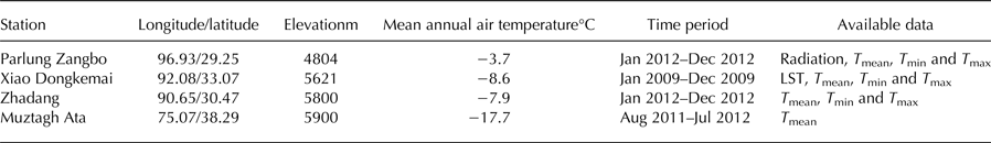
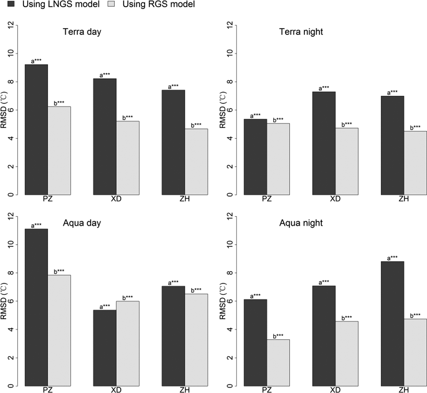
Figure 4 shows significant differences for T mean estimation using the RGS and LNGS models. The averaged RMSD of the LNGS model is 5.0°C, which is larger than 4.3°C of the RGS model. In particular, the performance improvement by replacing the LNGS model with the RGS model showed an RMSD decrease of 1.2 and 0.4°C for cases using MODIS daytime LST and night-time LST, respectively. Thus, the RGS models with better performance than the LNGS models were used for further analysis.
Comparison between the LNGS and RGS models for T mean estimation. ‘PZ’, Parlung Zangbo; ‘MA’, Muztagh Ata; ‘XD’, Xiao Dongkemadi; ‘ZH’, Zhadang. Asterisks indicate the significance of the differences: *** indicates 0.001 significance level; ** indicates 0.01 significance level; * indicates 0.05 significance level; letters without asterisks indicate insignificant differences.
The averaged RMSD of T air estimation from the TLR method was 5.2°C which is larger than 4.3°C of the RGS model based on MODIS LST (Fig. 5). In particular, RGS model based on MODIS night-time LST showed relatively high and stable accuracy with an averaged RMSD of 3.8°C, which is better than that of the TLR method. A fair comparison based on days with four available daily MODIS observations indicated that the RGS model based on MODIS night-time LST, with a mean RMSD of 3.3°C, is superior to the RGS model based on MODIS daytime LST, with a mean RMSD of 4.2°C (Fig. S2), for T mean estimation. The RGS model based on MODIS/Terra night-time LST presented the best performance with a mean RMSD of 3.0°C.
Comparison between the TLR method and the RGS model based on MODIS LST for T mean estimation. ‘TD’, Terra Day; ‘TN’, Terra Night; ‘AD’, Aqua Day; ‘AN’, Aqua Night. Asterisks indicate the significance of the differences: *** indicates 0.001 significance level; ** indicates 0.01 significance level; * indicates 0.05 significance level; letters without asterisks indicate insignificant differences.

Figure 5 also shows that the methods for T mean estimation based on MODIS LST clearly outperformed those using TLR except for Xiao Dongkemadi, where a high accuracy of ~2.1°C was obtained using the TLR method. However, the TLR method produced relatively low accuracies of 4.4–8.7°C at the other three glaciers, where higher accuracies of 2.7–7.5°C were obtained by the RGS model using MODIS LST, except for the RGS model based on Aqua daytime LST at Parlung Zangbo owing to the lower accuracies of LST (Figs 3, S1).
4.2.2. T min estimation
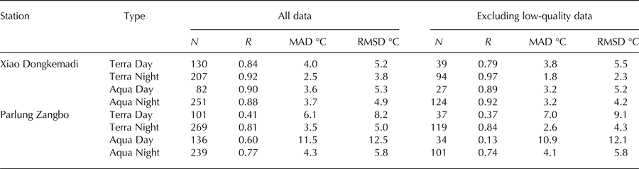
Similar to what was found in T mean estimation, the RGS and LNGS models showed significant differences for T min estimation with averaged RMSDs of 4.3 and 5.5°C, respectively (Fig. 6). The performance improvements between RGS and LNGS models were significant with RMSD decrease of 1.8 and 0.5°C for cases using MODIS daytime and night-time LST, respectively. This also indicates the necessity of applying the RGS model for T min estimation when using MODIS LST.
Comparison between the LNGS and RGS models for T min estimation. ‘PZ’, Parlung Zangbo; ‘XD’, Xiao Dongkemadi; ‘ZH’, Zhadang. Asterisks indicate the significance of the differences: *** indicates 0.001 significance level; ** indicates 0.01 significance level; * indicates 0.05 significance level; letters without asterisks indicate insignificant differences.
For most cases, significant differences were shown between methods using TLR and the RGS model based on MODIS LST (Fig. 7) with averaged RMSDs of 4.7 and 4.3°C for T min estimation, respectively. The RGS model based on MODIS night-time LST showed an even lower mean RMSD of 3.5°C. Days with four daily MODIS observations indicated that the RGS model based on MODIS night-time LST, with a mean RMSD of 3.0°C, is superior to the RGS model based on MODIS daytime LST, with a mean RMSD of 4.7°C for T min estimation (Fig. S3). The RGS model based on MODIS/Terra night-time LST presented the best case with a mean RMSD of 2.9°C.
Comparison between the TLR method and the RGS model based on MODIS LST for T min estimation. ‘TD’, Terra Day; ‘TN’, Terra Night; ‘AD’, Aqua Day; ‘AN’, Aqua Night. Asterisks indicate the significance of the differences: *** indicates 0.001 significance level; ** indicates 0.01 significance level; * indicates 0.05 significance level; letters without asterisks indicate insignificant differences.

4.2.3. T max estimation
The RGS and LNGS models showed significant differences for T max estimation (Fig. 8). Both models produced obviously lower accuracies with higher averaged RMSDs of 5.3 and 7.5°C, respectively, compared with T mean (4.3 and 5.0°C) and T min (4.3 and 5.5°C) estimations. In addition, the performance improvements of the RGS model compared with the LNGS model for cases using MODIS daytime and night-time LST, with RMSD decreases of 2.0 and 2.5°C, respectively, were both relatively large.
Comparison between the LNGS and RGS models for T max estimation. ‘PZ’, Parlung Zangbo; ‘XD’, Xiao Dongkemadi; ‘ZH’, Zhadang. Asterisks indicate the significance of the differences: *** indicates 0.001 significance level; ** indicates 0.01 significance level; * indicates 0.05 significance level; letters without asterisks indicate insignificant differences.
The TLR method and the RGS model based on MODIS LST showed significant differences in T max estimation for all cases (Fig. 9), which is consistent with T mean and T min. The averaged RMSD of 5.9°C for the TLR method is comparable with 5.3°C for the RGS model using MODIS LST. The RGS model based on MODIS night-time LST showed relatively better performance with an averaged RMSD of 4.5°C, whereas the accuracies are remarkably lower than those of T mean and T min estimation. As shown in Figure S4, a fair comparison based on days with four daily MODIS observations indicated that the RGS model based on MODIS night-time LST, with a mean RMSD of 4.8°C, is superior to that based on MODIS daytime LST, with a mean RMSD of 5.7°C for T max estimation. The RGS model based on MODIS/Aqua night-time LST with a mean RMSD of 4.5°C performed the best.
Comparison between the TLR method and the RGS model based on MODIS LST for T max estimation. ‘TD’, Terra Day; ‘TN’, Terra Night; ‘AD’, Aqua Day; ‘AN’, Aqua Night. Asterisks indicate the significance of the differences: *** indicates 0.001 significance level; ** indicates 0.01 significance level; * indicates 0.05 significance level; letters without asterisks indicate insignificant differences.
5. DISCUSSION
5.1. Limitations of MODIS LST on glacier surfaces of the TP
5.1.1. MODIS night-time LST
A clear cold bias frequently occurs at night for MODIS LST. This was particularly true for MODIS/Aqua night-time LST at the Parlung Zangbo, resulting in the maximum error among all four MODIS night-time LST terms (Table 2). This can be largely explained by deficiencies in the MODIS night-time cloud-detecting algorithm (Ackerman and others, Reference Ackerman1998). A relatively large proportion of undetected clouds exists in MODIS night-time LST (Østby and others, Reference Østby, Schuler and Westermann2014; Zhang and others, Reference Zhang, Zhang, Zhang, He and Tian2016b). When undetected cloud pixels exist, cloud top temperatures will take the place of true LSTs, resulting in much lower values. A cold bias of more than 10°C existed in up to 38 cases of MODIS night-time LST observed at the Parlung Zangbo. Such large errors resulted from undetected clouds have also been observed in other regions (Langer and others, Reference Langer, Westermann and Boike2010; Westermann and others, Reference Westermann, Langer and Boike2011, Reference Westermann, Langer and Boike2012).
5.1.2. MODIS daytime LST
During the daytime, obvious warm bias existed for many cases, and almost throughout the year for Aqua daytime LST observed at Parlung Zangbo, which resulted in extremely large errors (Fig. 3). This result can be partly explained by the possible failure in atmospheric correction, as indicated by Østby and others (Reference Østby, Schuler and Westermann2014). It should be noted that MODIS daytime LST is also affected by undetected clouds (Williamson and others, Reference Williamson, Hik, Gamon, Kavanaugh and Koh2013), although such influence is significantly smaller than for MODIS night-time LST (Ackerman and others, Reference Ackerman1998; Zhang and others, Reference Zhang, Zhang, Zhang, He and Tian2016b). Hall and others (Reference Hall, Williams, Luthcke and Digirolamo2008b) also discussed other possible reasons such as the mixed-pixel effect of melting water ponds within the pixel. However, this factor was less likely to be the dominant factors in the present study. Figure 10 plots the heterogeneity of MODIS pixel used. The variability of altitudes within pixels of the Xiao Dongkemadi and the Parlung Zangbo stations was small with standard errors of only 75 and 63 m, respectively. However, a relatively large proportion of non-glacier areas was covered within both MODIS pixels with fractions of 28 and 32% for Xiao Dongkemadi and Parlung Zangbo, respectively. During the day, LST is generally higher than T air, whereas LST on glacier surfaces cannot exceed the melting point (e.g. 0°C) (Hall and others, Reference Hall, Williams, Casey, DiGirolamo and Wan2006) even when T air is above 0°C. Thus, daytime enhances the strong LST difference between glacier and non-glacier area within MODIS pixels, especially in warm seasons. Similarly, obvious temperature differences of >10°C are observed between snow and snow-free surfaces in summer over a high-arctic tundra (Westermann and others, Reference Westermann, Langer and Boike2011). Therefore, the warm-bias errors for our study may be largely attributed to pixel heterogeneity.
Distribution of land covers and elevations within MODIS pixels at four glacier AWSs. Land covers (upper) are described by Landsat images observed during the time period of data used in this study. Elevation (lower) information within MODIS pixels are drawn from ASTER GDEM dataset (http://gdem.ersdac.jspacesystems.or.jp/).

5.1.3 Comparison with other evaluation or validation studies
Previous validation over the TP has focused mainly on areas with vegetated land cover. Yu and Ma (Reference Yu and Ma2011) obtained RMSD values of 3.1–5.3°C across three test sites with different land cover types (farm land, forest and desert grassland) in the northeastern TP. Min and others (Reference Min, Yueqing and Zhou2015) found a general RMSD of 5.3°C at an alpine meadow-dominated station in the eastern TP. Wang and Min (Reference Wang and Min2014) obtained an RMSD of 2.2°C for MODIS night-time LST observed at the Linzhi area in the southeastern TP. All of these studies included problems of pixel heterogeneity to varying degrees. However, our study featured obviously higher errors in MODIS daytime LST owing to the strong contrast between glacier and non-glacier area within MODIS pixels, especially at Parlung Zangbo.
Compared with validation studies for glacier/ice surfaces in the Arctic (Østby and others, Reference Østby, Schuler and Westermann2014) and Greenland (Hall and others, Reference Hall2008a, Koenig and Hall, Reference Koenig and Hall2010) areas, where ice surfaces are relatively homogeneous, an obviously larger warm bias for MODIS daytime LST was found in this study owing to the strong pixel heterogeneity. In the TP, glaciers are generally small (<1 km2) (Guo and others, Reference Guo2014). The mixed-pixel problem is a known limitation in MODIS LST observation; downscaling is needed for future studies on glacier surfaces of the TP using MODIS LST.
Despite the larger RMSDs for MODIS daytime LST than those reported in previous studies (Wan and others, Reference Wan, Zhang, Zhang and Li2002; Coll and others, Reference Coll2005), the evaluation results of MODIS night-time LST are generally consistent with them (Bosilovich, Reference Bosilovich2006; Wang and others, Reference Wang, Liang and Meyers2008; Wang and Liang, Reference Wang and Liang2009; Li and others, Reference Li2014; Krishnan and others, Reference Krishnan2015). The minimum RMSDs of the Xiao Dongkemadi and the Parlung Zangbo stations were only 2.3 and 4.3°C, respectively, which is within the range of 2.2–4.6°C observed for MODIS night-time LST over the TP (Yu and Ma, Reference Yu and Ma2011; Wang and Min, Reference Wang and Min2014; Min and others, Reference Min, Yueqing and Zhou2015). The night-time LST could be more homogeneous within the pixels due to the absence of large uncertainty introduced by solar radiation at daytime (Wang and others, Reference Wang, Liang and Meyers2008; Yu and Ma, Reference Yu and Ma2011).
5.1.4. Data quality
To further evaluate the effects of MODIS-claimed QC flags, the evaluation excluding low-quality data (i.e. QC > 1) was also examined (Table 2). Except for the clear improvement for Terra night-time LST observed at Xiao Dongkemadi, generally comparable accuracies or limited improvements can be obtained after removing the suspicious data. This indicates the dominating effect of pixel heterogeneity for MODIS daytime LST and also reveals the fact that undetected clouds may still exist after removing the low-quality data. It should be noted that removing the suspicious data can largely reduce the available sample amounts.
5.2. Comparison between the RGS and LNGS models
The RGS models showed consistently higher accuracies than the LNGS models for estimations of T mean, T min and T max (Figs 4, 6, 8). This indicates that there may be strong differences of T air–LST relationship between glacier and non-glacier surfaces, and RGS models should be used on glacier surfaces. It should be noted that the LNGS model was trained using samples from non-glacier stations and validated using observations from glacier stations. Due to the large variation of elevation among non-glacier stations, we also tried to add the elevation information to LNGS model to test if it could get higher accuracies, and such LNGS models are built as:
 $$T_{{\rm air}} = a + b \times {\rm LST} + c \times Z,$$
where LST is MODIS LST data including four instantaneous observations as mentioned before; Z is elevation; a, b and c are all regression coefficients. However, after adding the factor of elevation, the LNGS models produced even lower accuracies (Fig. S5). This may be because the temperature variation with altitude is discontinuous between glacier- and non-glacier surfaces (Wang and others, Reference Wang, Jian-Qiao, Hong-Bo and Zhen2013a); thus, such effects derived from non-glacier observations may be strongly biased for glacierized areas and lead to more errors.
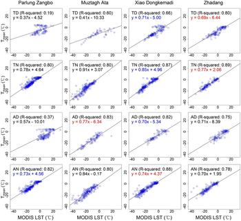
Figure 11 shows the regression models between T air of AWSs and MODIS LST at four pass times at different glaciers. For each MODIS pass time, differences were noted among models of the four glaciers, which indicates that different models may need to be built for obtaining locally accurate estimations on glacier surfaces. However, obtaining sufficient T air observations on individual glacier surface is extremely difficult. In addition, the performances of fixed models, especially those based on Terra night-time LST, built at a given glacier AWS shows highly acceptable validation results at the other glaciers (Figs 5, 7, 9). This indicates that the T air–LST relationship may not vary greatly among different glacier sites and the RGS models are recommended for T air estimation.
Linear regression between T mean and MODIS LST at four glacier AWSs. The coefficients of determination (R 2) and equations are shown at top-left in each sub-plot. Equations in red colors indicate the best models and those in blue colors indicate the second-best models for different MODIS pass times. ‘TD’, Terra Day; ‘TN’, Terra Night; ‘AD’, Aqua Day; ‘AN’, Aqua Night.
5.3. Implications, uncertainties and future developments for T air estimation using MODIS LST in glacierized areas over the TP
Both MODIS daytime and night-time LST have shown relatively good performances in T air estimation in many mountainous areas around the world including the TP (Zhang and others, Reference Zhang, Huang, Yu and Sun2011, Reference Zhang, Zhang, Ye, Che and Zhang2016a, Benali and others, Reference Benali, Carvalho, Nunes, Carvalhais and Santos2012). Problems such as obvious warm bias were identified with MODIS daytime LST in glacierized areas as shown in this study. We attribute its evident deficiency to the mixed-pixel problem resulting from strong temperature heterogeneity in the daytime. This problem affects the performance of MODIS daytime LST in T air estimation. However, MODIS night-time LST showed much lower bias than MODIS daytime LST in glacierized regions. Thus, MODIS night-time LST are strongly recommended in glacierized areas of the TP.
Terra night-time LST appeared to be more reliable than Aqua night-time LST illustrated by the higher accuracies in T air estimation (Fu and others, Reference Fu2011; Zhang and others, Reference Zhang, Huang, Yu and Sun2011). Generally lower bias of Terra LST than Aqua LST was found in this study (Section 4.1) and other validation studies of the TP (Yu and Ma, Reference Yu and Ma2011; Min and others, Reference Min, Yueqing and Zhou2015). Thus, the RGS models based on Terra night-time LST are recommended for T air estimation (Figs 11, S6 and S7).
Our study indicates that the best accuracies of T mean and T min estimation using MODIS LST, with RMSDs of 3.0 and 2.9°C, respectively, are clearly higher than that of T max estimation, with an RMSD of 4.5°C. This result is consistent with those reported in other studies (Benali and others, Reference Benali, Carvalho, Nunes, Carvalhais and Santos2012; Good, Reference Good2015); however, the reported performance differences at ~1.5°C are larger and the accuracies of T max estimation are obviously lower than those in other regions (Zhang and others, Reference Zhang, Huang, Yu and Sun2011; Xu and others, Reference Xu, Knudby and Ho2014; Oyler and others, Reference Oyler, Dobrowski, Holden and Running2016). T max occurs during the day; therefore, clouds can greatly affect the accuracies of MODIS LST (Williamson and others, Reference Williamson, Hik, Gamon, Kavanaugh and Koh2013) as well as the T air–LST relationship (Zhang and others, Reference Zhang, Zhang, Zhang, He and Tian2016b). In addition, the lower accuracy of T max estimation can be largely attributed to the strong influence of pixel heterogeneity on daytime LST. Future studies may need to develop advanced downscale methods for obtaining more accurate and fine LST data on glacier surfaces. It should be noted that compared with this study, a much larger RMSD was found for air temperature estimation from MODIS LST in the Antarctic (Meyer and others, Reference Meyer2016) where ice sheets are widespread, which may be largely due to: (1) Antarctic area has more extremely low temperatures (<−35°C) which are hard to predict (Meyer and others, Reference Meyer2016); (2) the accuracies reported from their study are actually for instaneous air temperatures, whereas those from this study focus on daily air temperatures.
Undetected clouds present in MODIS night-time LST have obviously negative effects on T air estimation (Zhang and others, Reference Zhang, Zhang, Zhang, He and Tian2016b). The estimation accuracies using MODIS LST can be greatly improved by screening samples (Zhang and others, Reference Zhang, Zhang, Zhang, He and Tian2016b). In addition, removing suspicious data based on MODIS claimed QC flags can also contribute to more accurate estimation (Williamson and others, Reference Williamson, Hik, Gamon, Kavanaugh and Koh2013; Zhang and others, Reference Zhang, Zhang, Ye, Che and Zhang2016a). This option was not used in the present study owing to limited T air observations from glacier AWSs. Future study is needed to obtain additional ground measurements at glacier surfaces and to build more reliable and accurate models for glacierized regions. In addition to LST, other variables including latitude, longitude, elevation, Julian day and solar zenith have been used in several studies to improve the estimation accuracies (Benali and others, Reference Benali, Carvalho, Nunes, Carvalhais and Santos2012; Xu and others, Reference Xu, Qin and Shen2012; Janatian and others, Reference Janatian2016; Zhang and others, Reference Zhang, Zhang, Ye, Che and Zhang2016a). Owing to the relatively short time series of T air observations and the limited number of stations, some variables including latitude, longitude and elevation were not used in this study. The Julian day was tested as an auxiliary variable and only slight improvements were achieved with the RMSD decrease of <0.01°C. Future research may benefit from including more efficient auxiliary variables.
5.4. MODIS LST vs TLR for T air estimation in glacierized basins
5.4.1. Uncertainty of TLR
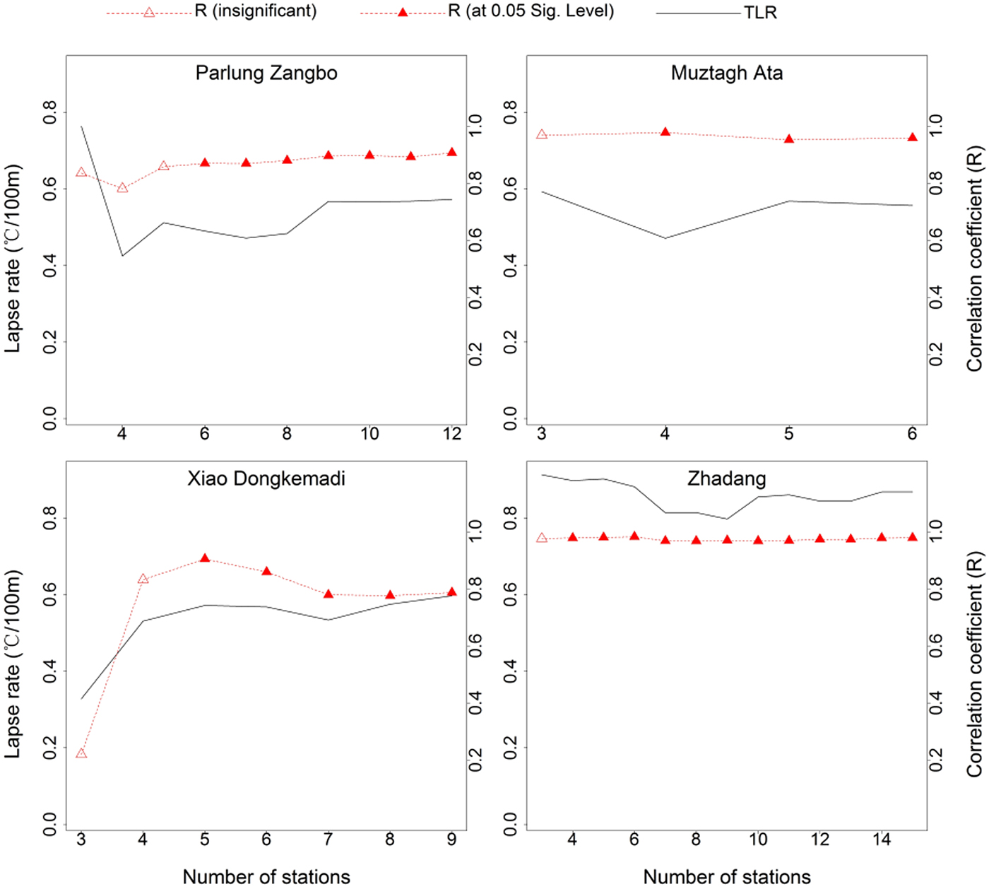
TLR is often assumed to have a constant value of ~0.65°C/100 m in glacierized regions (Hock and Holmgren, Reference Hock and Holmgren2005; Arnold and others, Reference Arnold, Rees, Hodson and Kohler2006; Machguth and others, Reference Machguth, Paul, Hoelzle and Haeberli2006). However, several studies have reported that TLR is not a spatial or temporal constant owing to variability in the microclimatic conditions (Rolland, Reference Rolland2003; Li and others, Reference Li2013a). In this study, the spatial representativeness of TLR was considered through sensitivity tests. Figure 12 shows that the TLR of T mean can vary substantially depending on the number of neighboring stations. When the number is small, only insignificant lapse rates and relatively weak R can be obtained. A high correlation coefficient of ~0.8 between T air and elevation appeared when station number was big enough; however, TLR still changed with a relatively large variation as the station number kept increasing. The first value of station number that passed the 0.05 significance test was chosen (Fig. 12); and these values are 6 for the Parlung Zangbo, 5 for the Xiao Dongkemadi, 4 for the Zhadang and 4 for the Muztagh Ata stations, respectively. We also conducted the sensitivity tests for T min and T max and achieved similar results. Finally, for each AWS, the annual mean air temperature shows generally good negative correlation with elevation among the neighboring stations selected (Fig. 2b). The temporal variation of TLR was also analyzed in this study. Monthly TLR was selected because it generally has higher accuracy than daily TLR. In this study for T mean interpolation, the averaged RMSE produced using monthly TLR (5.2°C) was found to be smaller than that using daily TLR (5.9°C). This may be because fluctuations in microclimates may affect the general pattern of TLR.
Sensitivity tests on number of stations for estimating TLR of T mean.
TLR can be affected by microclimatic conditions such as terrains, humid conditions and valley winds in various mountainous regions around the world (Rolland, Reference Rolland2003; Minder and others, Reference Minder, Mote and Lundquist2010), including the TP (Li and Xie, Reference Li and Xie2006; Kattel and others, Reference Kattel2013; Liu and others, Reference Liu2013). In particular, the temperature inversion in high-altitude or glacierized regions adds more complexity (Nilsson, Reference Nilsson2009; Li and others, Reference Li2013a). Strong differences between the TLRs of low- and high-altitude regions have also been reported in the TP (Liu and others, Reference Liu2013). Limited high-altitude stations may introduce large errors (Immerzeel and others, Reference Immerzeel, Petersen, Ragettli and Pellicciotti2014). The TLR at the glacier surface may be clearly different from that in non-glacierized regions (Nilsson, Reference Nilsson2009). Our study confirmed that large estimation errors can be introduced at the glacier surface over the TP based on TLR derived from low-altitude stations.
5.4.2. Implications for selection of T air estimation from TLR or MODIS LST in glacierized areas
Both TLR (Stahl and others, Reference Stahl, Moore, Floyer, Asplin and McKendry2006; Zhang and others, Reference Zhang2015) and MODIS LST (Benali and others, Reference Benali, Carvalho, Nunes, Carvalhais and Santos2012; Zhang and others, Reference Zhang, Zhang, Ye, Che and Zhang2016a) have shown good performance in T air estimation in mountainous areas. In glacierized areas, MODIS/Terra night-time LST showed highly acceptable performances in T air (T mean and T min) estimation, which were generally better than TLR in most cases as shown in the present study.
The most evident deficiency of MODIS LST is the missing data owing to cloud blockage (Yu and others, Reference Yu2016; Zhang and others, Reference Zhang, Zhang, Ye, Che and Zhang2016a; Zhu and others, Reference Zhu, Lű, Jia, Yan and Mahmood2017). Interpolation for MODIS LST may introduce more uncertainties although some advanced methods have been developed (Xu and Shen, Reference Xu and Shen2013; Yu and others, Reference Yu, Wu, Nan, Zhao and Wang2014). In addition, the problems of undetected clouds, data quality and mixed pixels may also introduce errors. The TLR based on meteorological stations in glacierized areas may generate more accurate T air estimation. However, MODIS LST is strongly recommended for T air estimation in glacierized areas where stations are sparse.
It should be noted that this study is not intended to negate the importance of TLR; we also tested performance for stations located in non-glacierized regions. The TLR method showed comparable performance in T air estimation compared with that using MODIS LST (Fig. S8). This indicates that if station networks are sufficiently dense and the produced TLR is locally reliable, TLR is an efficient method and is highly recommended because of its simple concept and ease of use. However, MODIS LST can be a good alternative for more accurate T air estimation in glacierized basins where high-altitude stations are too scarce to generate locally reliable TLR.
6. CONCLUSION
In this study, MODIS LST data were used for T air (T mean, T min and T max) estimations. The performances were evaluated by comparing with actual T air observations as well as with the results produced by the TLR method. Since careful validation is the basis of efficient application of remotely sensed LST, MODIS LST data were first compared with in-situ LST measurements of AWSs at two glaciers. The comparison results indicated that MODIS daytime LST data may have large errors (with mean RMSD of 8.0°C) on glacier surfaces of the TP likely owing to the mixed-pixel problem. In comparison, MODIS night-time LST (with mean RMSD of 4.0°C), especially MODIS/Terra night-time LST (with mean RMSD of 3.3°C), shows much lower bias. It was found that the selected regression models built at the RGS for the estimation of T air showed higher accuracy than those at LNGS. The performances of the RGS models based on MODIS night-time LST with mean RMSDs of 3.3, 3.0 and 4.8°C, were all obviously better than those of the RGS models based on MODIS daytime LST with mean RMSDs of 4.2, 4.7 and 5.7°C for the estimations of T mean, T min and T max on glacier surfaces of the TP, respectively. The accuracies of T mean and T min estimations were significantly higher than those of T max estimation using MODIS LST. Compared with the TLR method (with mean RMSDs of 5.2, 4.7 and 5.9°C for T mean, T min and T max estimations, respectively), the RGS models based on MODIS night-time LST produced better accuracies. Thus, regression using MODIS night-time LST can be a good alternative method for TLR for more accurate T air estimation in glacierized areas in the TP.
SUPPLEMENTARY MATERIAL
The supplementary material for this article can be found at https://doi.org/10.1017/jog.2018.6.
ACKNOWLEDGEMENTS
This study was supported by the National Natural Science Foundation of China (grant No. 41371087 and 41701079), and the China Postdoctoral Science Foundation (grant No. 2017M611013). We thank the Tanggula Station for Cryosphere Environment Observation and Research (supported by the National Natural Science Foundation of China grant No. 41271079 and 41130638), the Southeast Tibetan Plateau Station for Integrated Observation and Research of Alpine Environment, the Muztagh Ata Station for Westerly Environment Observation and Research and the Nam Co Station for Multisphere Observation and Research for providing ground measurements of longwave radiation and air temperature data. In addition, we are grateful to the Chinese Meteorology Administration (http://data.cma.cn/) for providing air temperature data. The MODIS LST products can be downloaded at no charge from the Reverb website (http://reverb.echo.nasa.gov/).


 Open access