





1 Introduction
Bayesian methods have long received attention in psychometrics, and they have been increasingly used in recent times. Martin and McDonald (Reference Martin and McDonald1975) were among early researchers who considered Bayesian methods, employing prior distributions to avoid Heywood cases in factor analysis. Other early approaches come from Bartholomew (Reference Bartholomew1981), Lee (Reference Lee1981), and Press (Reference Press1972). Lee, Song, and colleagues later made many additional developments involving Gibbs samplers (Lee, Reference Lee2007; Lee & Song, Reference Lee and Song2002; Lee et al., Reference Lee, Song and Tang2007; Shi & Lee, Reference Shi and Lee1997, Reference Shi and Lee1998; Song & Lee, Reference Song and Lee2001, Reference Song and Lee2012) with other notable works, including Arminger and Muthén (Reference Arminger and Muthén1998), Scheines et al. (Reference Scheines, Hoijtink and Boomsma1999), Patz and Junker (Reference Patz and Junker1999a, Reference Patz and Junker1999b), Edwards (Reference Edwards2010), Fox (Reference Fox2010), and Fox and Glas (Reference Fox and Glas2001). Much of this research happened in the late 1990s and early 2000s, which was also the height of WinBUGS (Lunn et al., Reference Lunn, Jackson, Best, Thomas and Spiegelhalter2012). WinBUGS the first major piece of software to provide flexible and accessible MCMC methods to applied researchers, with specific psychometric applications coming from Curtis (Reference Curtis2010), Lee et al. (Reference Lee, Song and Tang2007), and Zhang et al. (Reference Zhang, Hamagami, Wang, Nesselroade and Grimm2007), among others. WinBUGS also inspired psychometric model checking procedures from Glas and Meijer (Reference Glas and Meijer2003) as well as Sinharay and colleagues (Sinharay, Reference Sinharay2004, Reference Sinharay2005; Sinharay et al., Reference Sinharay, Johnson and Stern2006).
Despite the above work, Bayesian psychometric modeling was a relatively niche research area through the early 2000s. The Bayesian skepticism held by many 20th century statisticians (e.g., Breiman, Reference Breiman1997) was also held by some psychometricians during that time. A notable change happened when Bayesian functionality was introduced to Mplus (Muthén & Muthén, 1998–Reference Muthén and Muthén2017) around 2010. The implementations and accompanying articles (Asparouhov & Muthén, Reference Asparouhov and Muthén2010; Muthén & Asparouhov, Reference Muthén and Asparouhov2012) helped researchers see the advantages that Bayesian methods hold for complex models, though some expressed appropriate levels of skepticism (e.g., MacCallum et al., Reference MacCallum, Edwards and Cai2012; Stromeyer et al., Reference Stromeyer, Miller, Sriramachandramurthy and DeMartino2015). Today, Bayesian modeling appears to have a general level of acceptance among the psychometric community. Among other topics, researchers have been active in developing models for intensive time series (e.g., Asparouhov et al., Reference Asparouhov, Hamaker and Muthén2018; Chen et al., Reference Chen, Chow, Oravecz and Ferrer2023; Driver et al., Reference Driver, Oud and Voelkle2017; Rast et al., Reference Rast, Martin, Liu and Williams2022; Roman & Brandt, Reference Roman and Brandt2021; Woźniak, Reference Woźniak2024), in studying prior distributions (e.g., Bainter, Reference Bainter2017; Kaplan et al., Reference Kaplan, Chen, Yavuz and Lyu2023; Liu et al., Reference Liu, Zhang and Grimm2016; Lu et al., Reference Lu, Chow and Loken2016; Padgett & Winter, Reference Padgett and Winter2025; Padgett et al., Reference Padgett, Morgan and Lomas2024; Pokropek et al., Reference Pokropek, Schmidt and Davidov2020; Van Erp & Browne, Reference Van Erp and Browne2021; Van Erp et al., Reference Van Erp, Mulder and Oberski2018; Van Zundert et al., Reference Van Zundert, Somer and Miočević2022), and in developing model assessment tools (e.g., Cain & Zhang, Reference Cain and Zhang2018; Depaoli et al., Reference Depaoli, Lai and Yang2021; Fox et al., Reference Fox, Mulder and Sinharay2017; Garnier-Villarreal & Jorgensen, Reference Garnier-Villarreal and Jorgensen2020; Hoijtink & van de Schoot, Reference Hoijtink and van de Schoot2018; Liu et al., Reference Liu, Depaoli and Marvin2022; Uanhoro, Reference Uanhoro2023; Verhagen & Fox, Reference Verhagen and Fox2013; Winter & Depaoli, Reference Winter and Depaoli2022, Reference Winter and Depaoli2023; Zhang et al., Reference Zhang, Tao, Wang and Shi2019, Reference Zhang, Templin and Mintz2022). Much of this work makes use of the fact that traditional Bayesian methods are often easily extended to handle incomplete datasets and to relax model assumptions (e.g., Cai et al., Reference Cai, Lee and Song2008; Jorgensen et al., Reference Jorgensen, Forney, Hall and Giles2018; Lee & Xia, Reference Lee and Xia2008; Merkle, Reference Merkle2011; Tong & Zhang, Reference Tong and Zhang2020; Zhang et al., Reference Zhang, Lai, Lu and Tong2013, Reference Zhang, Li and Liu2014).
Despite the popularity of Bayesian methods in psychometrics, the intuition underlying popular estimation methods is sometimes lacking, and psychometricians are sometimes reluctant to engage with the technical details underlying the estimation methods. Some of this reluctance is probably due to the relevant literature, which can present disparate results without providing context about where the results come from. This is understandable, as psychometrics researchers often apply established results from statistics to psychometric models. But it also leads to difficulties for researchers who are new to Bayesian psychometrics, because they must become familiar with a body of Bayesian statistics literature in addition to the psychometrics literature. The goal of this article is to synthesize popular procedures and results related to MCMC estimation of psychometric models, and to provide intuition about where the results come from and how they can be implemented. We discuss a unified regression-based framework that covers many popular psychometric models, including factor analysis, path models, growth models, structural equation models (SEMs), and some item response models. Near the end of the article, we also consider how this framework informs other psychometric models that are not covered.
In combining major results related to Gibbs samplers as well as Hamiltonian samplers, this article is intended to be a reference for psychometrics researchers on popular Bayesian estimation methods as well as an entrance to psychometric models for statistics researchers. We aim to provide the core results needed to implement popular MCMC methods while simultaneously providing enough intuition to understand popular MCMC methods. We assume some general background in statistical methods and linear algebra, with the article potentially being useful to different readers depending on their specific background. For example, readers who are familiar with SEM but not with Bayesian methods may elect to skip over some model definitions. Readers who are familiar with Bayesian methods but not SEM might spend more time on the model definitions, and they might find the comparisons between regression and SEM to be especially useful. Readers who are already familiar with Bayesian methods and SEM may skip directly to sections on Gibbs sampling or on Hamiltonian sampling, each of which provide a good deal of results for reference.
In the following pages, we first provide a conceptual overview of Bayesian estimation, emphasizing the geometry of the posterior distribution. This is helpful for building an intuition about how Bayesian estimation works. We then provide details about traditional Gibbs samplers for regression, which we build upon in describing Gibbs samplers for SEM. Next, we transition to a discussion of Hamiltonian Monte Carlo (HMC), focusing on key ideas and intuition that are important for implementing HMC. Next, we consider how our regression-based framework informs item response and other psychometric models.
2 Bayesian background
We begin with a brief overview of traditional Bayesian ideas. For a book-length, introductory treatment, see McElreath (Reference McElreath2018) or Kaplan (Reference Kaplan2023). For book-length treatments focusing on Bayesian psychometric models, see Depaoli (Reference Depaoli2021) or Levy and Mislevy (Reference Levy and Mislevy2017). Related computational approaches and resources include Bürkner (Reference Bürkner2021), Fazio and Bürkner (Reference Fazio and Bürkner2025), and Padgett (Reference Padgett2022), while Levy and McNeish (Reference Levy and McNeish2023) provide an accessible overview of different Bayesian philosophies.
2.1 General ideas
In Bayesian modeling, we generally wish to learn about the posterior distribution of model parameters. The posterior distribution tells us about likely values of model parameters, and it can be summarized via point estimates, interval estimates, or other functions of parameters. Mathematically, the posterior distribution is proportional to the product of the model likelihood and the prior distribution. The model likelihood is the same as the likelihood used in frequentist estimation (i.e., it is the “likelihood” in “maximum likelihood estimation”). The prior distribution represents our uncertainty about model parameters before we observe data.
It is important to realize that the posterior distribution is just another probability distribution. We can visualize it for simple models, which can help us build an intuition for more complex models. Figure 1 shows a hypothetical posterior distribution for a model with two parameters, say, an intercept and a slope. Visualization of the distribution requires three dimensions: one for each parameter, and one for the value of the posterior distribution at each combination of parameter values. Figure 1 is arranged as if we are looking down on the posterior distribution; that is, we are flying over a mountain and looking down at it. The x-axis represents the intercept, the y-axis represents the slope, and the colors represent the height of the posterior distribution. Yellow-green is around the peak of the mountain, representing the most likely combinations of intercepts and slopes. Light purple is the bottom of the mountain, representing unlikely combinations of model parameters. Similar ideas apply to models with more than two parameters, but we cannot visualize the associated distributions because we live in a three-dimensional world.
Plot of hypothetical posterior distribution. The black point in the center is the peak of the posterior distribution. The line is a sequence of three samples from the posterior distribution.

Figure 1 Long description
The plot displays Intercept on the x-axis, ranging from 35 to 55, and Slope on the y-axis, ranging from 2.0 to 3.5. At the center is a black dot marking the peak of the posterior distribution, located near Intercept 45 and Slope 3.0. Surrounding this point are six concentric, colored contour bands representing decreasing posterior density outward from the center. In the lower left quadrant, three sample points are labeled 1, 2, and 3. Point 1 is at approximately Intercept 39, Slope 2.4; point 2 is at Intercept 41, Slope 2.7; point 3 is at Intercept 45, Slope 2.6. These points are connected sequentially by straight black lines, forming a path that first rises and then moves rightward. The contours are colored from yellow-green at the center to purple at the outermost band.
To learn about the posterior distribution in Figure 1, we might want to know the value of the intercept and slope at the peak of the mountain. We could use popular optimization methods like Newton–Raphson to find these values, and we might call the values “maximum a posteriori” (MAP) estimates or “posterior modes.” In Figure 1, the maximum occurs at the black point, which is an intercept of 45 and a slope of 3.
2.2 Posterior sampling
While the MAP estimates are useful summaries of the posterior distribution, we often want to learn about the entire distribution, which requires multiple summaries. To accomplish this, we can employ Markov chain Monte Carlo (MCMC) methods. Instead of directly trying to find the intercept and slope at the peak, we draw thousands of random samples from the distribution in Figure 1, where the probability of drawing each sample is related to the height of the posterior distribution. The mean of those random samples (one mean for each parameter) provides a summary of the posterior distribution’s center, and the standard deviation of the samples provides a summary of the posterior distribution’s variability. The random samples can lead us to many other summaries. For example, to estimate the probability that the intercept is greater than 50, we would simply calculate the proportion of intercept samples that are greater than 50.
While it is easy to say that we will draw random samples from the posterior distribution, the exact procedures for doing this are complicated. For some simple models, we can derive analytic results telling us that we should draw samples from a particular normal (or other) distribution. For complicated models, there are no analytic results telling us how to do this. But we still want to use MCMC to learn about the posterior distributions of those models.
In the latter cases, MCMC sampling generally proceeds as follows. We start with some initial values of model parameters. Based on those initial values, we jump to a new point of the posterior distribution in a particular manner and record the parameter values at that point. Now we repeat the process: based on our current location in the posterior distribution, we jump to another point and record the parameter values at that point. Then we keep going. These ideas are shown by the line in Figure 1. We start at the point labeled 1, which is an intercept of 38 and a slope of 2.4. This is in a low-density region of the posterior distribution (i.e., “off the mountain”) so represents unlikely parameter values. We then jump to the point labeled 2, which is an intercept of 42 and slope of 2.7 and is closer to the peak, as compared to point 1. We then jump to the point labeled 3, and we continue in this way until we visit thousands of points. Our posterior samples are the intercept and slope values that we visited along the way.
This simple example of sampling helps provide intuition for a variety of issues surrounding MCMC. First, our initial value was not particularly good. In practice, we will run the sampler for an initial burn-in period so that any influence of the initial value wears off. We discard the locations that we visited during the burn-in period, so we can be sure that the remaining locations are good representations of the posterior distribution. Second, MCMC samplers differ in how quickly they can travel to different parts of the posterior distribution. For example, some samplers may be unable to jump directly from point 1 to point 2, requiring a large number of intermediate samples to make it that far. This gets at the idea of sampling efficiency, which includes metrics involving autocorrelation and effective sample size. Efficient samplers can quickly travel around the posterior distribution, whereas inefficient samplers may require many thousands of samples to fully explore the posterior distribution.
Finally, while we can occasionally update all parameters simultaneously, we more often sample individual parameters or subsets of parameters sequentially. Considering the points labeled 1 and 2 in Figure 1, a simultaneous update entails moving directly from (38, 2.4) to (42, 2.7) in one go. In a sequential update, we might first update the intercept, providing an intermediate move from (38, 2.4) to (42, 2.4). We would then update the slope value from 2.4 to 2.7, conditioned on the intercept equaling 42. This sequential updating is the main idea of Gibbs sampling, and it is especially helpful for models with many parameters. Gibbs sampling allows us to break up the full set of parameters into subsets that are easier to handle. For each parameter subset, we sample from a conditional posterior distribution that conditions on values of the remaining parameters (those not in the subset). This conditioning allows us to apply some key results to many types of models, an idea we further explore in the next section.
3 Gibbs sampling of regression models
For reasons that will become apparent later, Bayesian methods for SEM rely heavily on Bayesian methods for regression. This section’s review of Bayesian regression results is intended to provide supports for the SEM results that come later. Our discussion generally follows that of Gelman et al. (Reference Gelman, Carlin, Stern, Dunson, Vehtari and Rubin2013).
3.1 Basics
A basic linear regression model of n responses can be written as

where
$\boldsymbol {y}$
 is an
$n \times 1$
is an
$n \times 1$
 vector of response variables,
$\boldsymbol {X}$
vector of response variables,
$\boldsymbol {X}$
 is an
$n \times m$
is an
$n \times m$
 design matrix, and
$\boldsymbol {\beta }$
design matrix, and
$\boldsymbol {\beta }$
 is the
$m \times 1$
is the
$m \times 1$
 vector of regression weights. The
$n \times n$
vector of regression weights. The
$n \times n$
 model covariance matrix,
$\sigma ^2 \boldsymbol {I}$
model covariance matrix,
$\sigma ^2 \boldsymbol {I}$
 , reflects the assumptions of independence and homogeneity: independence because all off-diagonal entries equal 0 (due to the identity matrix), and homogeneity because all diagonal entries equal
$\sigma ^2$
, reflects the assumptions of independence and homogeneity: independence because all off-diagonal entries equal 0 (due to the identity matrix), and homogeneity because all diagonal entries equal
$\sigma ^2$
 .
.
We first consider a Bayesian version of the model that includes flat, noninformative priors on
$\boldsymbol {\beta }$
 and
$\log (\sigma )$
and
$\log (\sigma )$
 , that is,

Under these priors, the conditional posterior distribution of
$\boldsymbol {\beta }$
 is
is

The mean of this distribution is especially intuitive, because it is the usual least squares estimate of
$\boldsymbol {\beta }$
 . The posterior distribution of
$\sigma ^2$
. The posterior distribution of
$\sigma ^2$
 can then be written in two ways, one that conditions on
$\boldsymbol {\beta }$
can then be written in two ways, one that conditions on
$\boldsymbol {\beta }$
 and one that is marginal over
$\boldsymbol {\beta }$
and one that is marginal over
$\boldsymbol {\beta }$
 :
:


The first line is most relevant to SEM, but the second line can lead to more efficient sampling. On the second line, the expression for the second parameter looks very involved, but it is just the usual sum of squared residuals in matrix form.
Now consider relaxing the independence and homogeneity assumptions of the covariance matrix. The model becomes

where the structure of the
$n \times n$
 matrix
$\boldsymbol {\Sigma }$
matrix
$\boldsymbol {\Sigma }$
 is unspecified. In this setting, the conditional posterior distribution of
$\boldsymbol {\beta }$
is unspecified. In this setting, the conditional posterior distribution of
$\boldsymbol {\beta }$
 now involves the full matrix
$\boldsymbol {\Sigma }$
now involves the full matrix
$\boldsymbol {\Sigma }$
 :
:

The conditional posterior distribution of
$\boldsymbol {\Sigma }$
 , on the other hand, depends on its exact form (e.g., known up to a scalar, equal off-diagonal entries, and unrestricted). For some cases, this conditional posterior distribution will not have a form from which it is easy to sample.
3.2 Informative priors
The results of the previous section used noninformative priors, which are often used in psychometrics. This reflects researchers’ reluctance to say that they know anything about model parameters before collecting data, perhaps because they view statistical models as yielding objective results that should not be unduly influenced. We think that researchers should use informative priors more often than they currently do. In considering reasonable prior distributions, it is often helpful to ask, “what are ridiculous values of model parameters that would never occur in practice?” This question leads us to the idea of weakly informative prior distributions (e.g., Chung et al., Reference Chung, Gelman, Rabe-Hesketh, Liu and Dorie2015; Gelman et al., Reference Gelman, Jakulin, Pittau and Su2008), which place most density on plausible values of model parameters. There is not one “correct” weakly informative prior distribution, which may worry researchers who seek objective results. But based on past experience, so long as the prior approximates “weakly informative,” its influence is less than other model choices, such as the number of latent variables, the nonzero entries of
$\boldsymbol {\Lambda }$
 and of
$\boldsymbol {B}$
and of
$\boldsymbol {B}$
 , and assumptions about conditional independence between observed variables. We acknowledge that the definition of “weakly informative” can become tricky for some complex models where the data do not provide much information about certain parameters. See Levy and Mislevy (Reference Levy and Mislevy2017, Chapter 3) for further discussion of prior distributions, which emphasizes the relationship between exchangeability, conditional independence, and prior distributions.
The previous paragraph might lead us to ask “if the prior is not very influential, why not stick with some form of noninformative prior?” There are a few responses to this question. First, from a pragmatic point of view, mildly informative priors help prevent the sampler from straying into low-density regions of the posterior and getting stuck. This issue is especially relevant to HMC methods, which are typically better at exploring the full posterior distribution as compared to Gibbs samplers. Second, mildly informative priors can reduce noise in metrics that involve the model’s log-likelihood, such as WAIC (Merkle et al., Reference Merkle, Furr and Rabe-Hesketh2019). This can allow researchers to draw sharp inferences about their data using fewer posterior samples. Third, noninformative priors do not guarantee that the priors for all functions of parameters are noninformative, which can cause unexpected problems (Seaman et al., Reference Seaman, Seaman and Stamey2012). Finally, mildly informative priors help methodologists take responsibility for their analyses (e.g., Rouder et al., Reference Rouder, Morey, Verhagen, Province and Wagenmakers2016). If we are to fit a model to data, we should know enough about the parameters beforehand to determine what values would be implausible.
Gelman et al. (Reference Gelman, Carlin, Stern, Dunson, Vehtari and Rubin2013) discuss how we can include informative priors (mildly informative or otherwise) for regression weights by augmenting the data with pseudo-observations representing the priors. Assume that the prior distribution is multivariate normal, that is,

which covers the situation where each individual regression weight is assigned a univariate normal prior distribution (in that case,
$\boldsymbol {\Sigma }_\beta $
 is diagonal). We can now define a new regression model

where the vectors and matrices with
$\ast $
 augment the model with parts of the prior. Specifically, we have

This formulation allows us to sample
$\boldsymbol {\beta }$
 using Equation (7), as if we had noninformative priors. We simply treat
$\boldsymbol {y}^\ast $
using Equation (7), as if we had noninformative priors. We simply treat
$\boldsymbol {y}^\ast $
 ,
$\boldsymbol {X}^\ast $
,
$\boldsymbol {X}^\ast $
 , and
$\boldsymbol {\Sigma }^\ast $
, and
$\boldsymbol {\Sigma }^\ast $
 as
$\boldsymbol {y}$
as
$\boldsymbol {y}$
 ,
$\boldsymbol {X}$
,
$\boldsymbol {X}$
 , and
$\boldsymbol {\Sigma }$
, and
$\boldsymbol {\Sigma }$
 in (7).
We now turn to the residual variance
$\sigma ^2$
 , when the model covariance matrix is specified as
$\sigma ^2 \boldsymbol {I}$
, when the model covariance matrix is specified as
$\sigma ^2 \boldsymbol {I}$
 . The conjugate prior for
$\sigma ^2$
. The conjugate prior for
$\sigma ^2$
 is the Inverse Gamma, where we denote the shape parameter as
$a_0$
is the Inverse Gamma, where we denote the shape parameter as
$a_0$
 and the scale parameter as
$b_0$
and the scale parameter as
$b_0$
 . Under this prior, we have

Now consider the case where the
$n \times n$
 residual covariance matrix
$\boldsymbol {\Sigma }$
residual covariance matrix
$\boldsymbol {\Sigma }$
 is unrestricted. The model now becomes overparameterized, but consideration of this situation becomes important for SEM. If
$\boldsymbol {\Sigma }$
is unrestricted. The model now becomes overparameterized, but consideration of this situation becomes important for SEM. If
$\boldsymbol {\Sigma }$
 is assigned an inverse-Wishart prior with degrees of freedom
$\nu _0$
is assigned an inverse-Wishart prior with degrees of freedom
$\nu _0$
 and scale matrix
$\boldsymbol {S}_0$
and scale matrix
$\boldsymbol {S}_0$
 , the posterior distribution is

In this expression, we add 1 to the degrees of freedom because the
$n \times 1$
 response vector
$\boldsymbol {y}$
response vector
$\boldsymbol {y}$
 is regarded as one observation that informs the
$n \times n$
is regarded as one observation that informs the
$n \times n$
 matrix
$\boldsymbol {\Sigma }$
matrix
$\boldsymbol {\Sigma }$
 .
.
4 Gibbs sampling of Bayesian SEM
Armed with our Gibbs sampler for heterogenous regression, we are now prepared to develop a Gibbs sampler for SEM. We first provide an explicit definition of the SEM, and we then see how the Gibbs sampler for SEM relies heavily on the Gibbs sampler for regression.
4.1 Model definition
We focus on the main lavaan (Rosseel, Reference Rosseel2012) representation of an SEM, which is related to the LISREL “all-y” representation (e.g., Jöreskog & Sörbom, Reference Jöreskog and Sörbom1997). This representation differs from some others (notably, Asparouhov & Muthén, Reference Asparouhov and Muthén2010) in how it handles exogenous observed variables. The other representations will separate exogenous observed variables from endogenous observed variables and assign them their own coefficient matrix (which is sometimes called
$\boldsymbol {K}$
 or
$\boldsymbol {\Gamma }$
or
$\boldsymbol {\Gamma }$
 ). In contrast, lavaan typically includes exogenous observed variables alongside other observed variables. More detail about this distinction appears in the Appendix.
Let
$\boldsymbol {y}_i$
 ,
$i = 1, \ldots , n$
,
$i = 1, \ldots , n$
 , be the p (continuous) observed variables associated with observation i. The traditional intent of the model is to describe the p observed variables by a smaller number of latent variables, similarly to how principal components compresses many observed variables into a single variable. But the SEM has a well-defined likelihood (as opposed to being an algorithm for data reduction), and it allows for regression relationships between latent variables. In traditional psychometric applications, the
$\boldsymbol {y}_i$
, be the p (continuous) observed variables associated with observation i. The traditional intent of the model is to describe the p observed variables by a smaller number of latent variables, similarly to how principal components compresses many observed variables into a single variable. But the SEM has a well-defined likelihood (as opposed to being an algorithm for data reduction), and it allows for regression relationships between latent variables. In traditional psychometric applications, the
$\boldsymbol {y}_i$
 are test scores and other observed variables about individuals, whereas the latent variables are unobserved traits such as “mathematics proficiency.”
An SEM with
$m < p$
 latent variables may be represented by the equations


where
$\boldsymbol {\eta }_i$
 is an
$m \times 1$
is an
$m \times 1$
 vector containing the latent variables;
$\boldsymbol {\epsilon }_i$
vector containing the latent variables;
$\boldsymbol {\epsilon }_i$
 is a
$p \times 1$
is a
$p \times 1$
 vector of measurement errors; and
$\boldsymbol {\zeta }_i$
vector of measurement errors; and
$\boldsymbol {\zeta }_i$
 is an
$m \times 1$
is an
$m \times 1$
 vector of structural errors. The vectors
$\boldsymbol {\nu }$
vector of structural errors. The vectors
$\boldsymbol {\nu }$
 and
$\boldsymbol {\alpha }$
and
$\boldsymbol {\alpha }$
 contain intercept parameters for the observed and latent variables, respectively;
$\boldsymbol {\Lambda }$
contain intercept parameters for the observed and latent variables, respectively;
$\boldsymbol {\Lambda }$
 is a matrix of factor loadings (regressions from latent to observed variables); and
$\boldsymbol {B}$
is a matrix of factor loadings (regressions from latent to observed variables); and
$\boldsymbol {B}$
 encodes regressions between latent variables.
Equation (11) is not always fully understood. It is peculiar because
$\boldsymbol {\eta }_i$
 appears on both the left and right side. To make sense of the equation, it is important to realize that the diagonal of
$\boldsymbol {B}$
appears on both the left and right side. To make sense of the equation, it is important to realize that the diagonal of
$\boldsymbol {B}$
 is fixed to 0, which means that no individual entry of
$\boldsymbol {\eta }_i$
is fixed to 0, which means that no individual entry of
$\boldsymbol {\eta }_i$
 is predicting itself. And nonzero, off-diagonal entries of
$\boldsymbol {B}$
is predicting itself. And nonzero, off-diagonal entries of
$\boldsymbol {B}$
 represent one entry of
$\boldsymbol {\eta }_i$
represent one entry of
$\boldsymbol {\eta }_i$
 being predicted by another entry of
$\boldsymbol {\eta }_i$
being predicted by another entry of
$\boldsymbol {\eta }_i$
 . The researcher specifies which off-diagonal entries are free and which off-diagonal entries are fixed to 0; the free entries represent paths (directed arrows) between latent variables in a path diagram. Similarly, the free entries of
$\boldsymbol {\Lambda }$
. The researcher specifies which off-diagonal entries are free and which off-diagonal entries are fixed to 0; the free entries represent paths (directed arrows) between latent variables in a path diagram. Similarly, the free entries of
$\boldsymbol {\Lambda }$
 in Equation (10) represent paths (directed arrows) from latent variables to observed variables.
The residuals
$\boldsymbol {\epsilon }_i$
 and
$\boldsymbol {\zeta }_i$
and
$\boldsymbol {\zeta }_i$
 are assumed to be multivariate normal:


where the associated covariance matrices are often diagonal. Taken together, these assumptions imply multiple distributions and likelihoods for the same model. Conditioned on the latent variables
$\boldsymbol {\eta }_i$
 , we have

If we instead integrate the
$\boldsymbol {\eta }_i$
 out of the model, we have

where we require that
$(\boldsymbol {I} - \boldsymbol {B})$
 is invertible.
There can be confusion about the conditional and marginal SEM distributions above. The confusion often stems from the idea that our one model has two different likelihoods associated with it. This means we could use either likelihood for Bayesian estimation, and we will obtain the same posterior distributions because both likelihoods come from the same model. For Bayesian estimation, we most commonly sample the latent variables
$\boldsymbol {\eta }_i$
 as model parameters, which relies on the conditional distribution in Equation (14). This is not absolutely required, though, and use of the conditional distribution can lead to inefficient HMC sampling (Merkle et al., Reference Merkle, Fitzsimmons, Uanhoro and Goodrich2021). For frequentist estimation, we usually rely on the marginal distribution from Equation (15) because the latent variables can lead to estimation difficulties, including the incidental parameter problem (e.g., Lancaster, Reference Lancaster2000).
4.2 Gibbs sampling of SEM
We now discuss Gibbs samplers of the above model, which are highly related to Gibbs samplers of regression models. A key idea is this: if the latent variables
$\boldsymbol {\eta }_i$
 were known, our SEM could be written as a regression model. And if our model can be written as a regression model, then the regression Gibbs sampler can be used to estimate our model.
To make this work, we need to know how to sample the
$\boldsymbol {\eta }_i$
 . This step is highly related to prediction of latent variables in frequentist models, and we review it in the next section. We then describe the full Gibbs sampler, which makes use of some results from Asparouhov and Muthén (Reference Asparouhov and Muthén2010).
4.2.1 Sampling latent variables
To sample latent variables
$\boldsymbol {\eta }_i$
 , we use standard properties of the multivariate normal distribution. We have (e.g., Jöreskog & Sörbom, Reference Jöreskog and Sörbom1997, p. 34) that the joint distribution of
$(\boldsymbol {y}_i^\prime \ \boldsymbol {\eta }_i^\prime )^\prime $
, we use standard properties of the multivariate normal distribution. We have (e.g., Jöreskog & Sörbom, Reference Jöreskog and Sörbom1997, p. 34) that the joint distribution of
$(\boldsymbol {y}_i^\prime \ \boldsymbol {\eta }_i^\prime )^\prime $
 is multivariate normal with mean

and covariance matrix

From this joint distribution, we can obtain the multivariate normal conditional distribution of
$\boldsymbol {\eta }_i$
 given
$\boldsymbol {y}_i$
given
$\boldsymbol {y}_i$
 . Using the Woodbury identity and others to simplify the expressions (e.g., Asparouhov & Muthén, Reference Asparouhov and Muthén2010), the mean of the conditional distribution is

and the covariance matrix is

This distribution is one piece of the Gibbs sampler. Conditioned on all model parameters except the
$\boldsymbol {\eta }_i$
 , we take draws from the above distribution. If we are using MCMC with the marginal likelihood (Equation (15); see Merkle et al., Reference Merkle, Fitzsimmons, Uanhoro and Goodrich2021), we could use the above distribution to sample the
$\boldsymbol {\eta }_i$
, we take draws from the above distribution. If we are using MCMC with the marginal likelihood (Equation (15); see Merkle et al., Reference Merkle, Fitzsimmons, Uanhoro and Goodrich2021), we could use the above distribution to sample the
$\boldsymbol {\eta }_i$
 as a post-estimation step, after sampling the other model parameters. As discussed later, this idea can be especially useful in HMC.
4.2.2 Sampling location parameters
Once the
$\boldsymbol {\eta }_i$
 have been sampled, we can use them to set up our regression model. The idea is to express Equations (10) and (11) in such a way that the free parameters in
$\boldsymbol {\nu }$
have been sampled, we can use them to set up our regression model. The idea is to express Equations (10) and (11) in such a way that the free parameters in
$\boldsymbol {\nu }$
 ,
$\boldsymbol {\Lambda }$
,
$\boldsymbol {\Lambda }$
 ,
$\boldsymbol {\alpha }$
,
$\boldsymbol {\alpha }$
 , and
$\boldsymbol {B}$
, and
$\boldsymbol {B}$
 are the regression weights.
Let
$\boldsymbol {\xi }$
 be a vector containing these free parameters. Then we can write Equations (10) and (11) as

where our design matrix
$\boldsymbol {H}_i$
 includes 1s for intercept parameters and entries of
$\boldsymbol {\eta }_i$
includes 1s for intercept parameters and entries of
$\boldsymbol {\eta }_i$
 that get multiplied by loadings and regression weights. So, for example, a CFA with three observed variables and one latent variable could be arranged as

where the final row consists of all zeros because the mean of the
$\boldsymbol {\eta }_i$
 is fixed to zero (which is typically the case, but not always). For structural models that include nonzero terms in
$\boldsymbol {\alpha }$
is fixed to zero (which is typically the case, but not always). For structural models that include nonzero terms in
$\boldsymbol {\alpha }$
 and/or in
$\boldsymbol {B}$
and/or in
$\boldsymbol {B}$
 , this final row may contain other latent variables that get paired with regression weights in
$\boldsymbol {B}$
, this final row may contain other latent variables that get paired with regression weights in
$\boldsymbol {B}$
 . Our multivariate normal covariance matrix,
$\boldsymbol {V}$
. Our multivariate normal covariance matrix,
$\boldsymbol {V}$
 , is then given as

With our model now set up as a regression, we can begin to see how to sample the model intercepts, loadings, and regression weights. But the model above is only for a single case i, and we want to use all cases in the data. To handle all cases, we keep adding to our regression model. We obtain

or more concisely,

where
$\boldsymbol {z}$
 includes the
$\boldsymbol {y}_i$
includes the
$\boldsymbol {y}_i$
 and
$\boldsymbol {\eta }_i$
and
$\boldsymbol {\eta }_i$
 in sequence, and the identity matrix
$\boldsymbol {I}$
in sequence, and the identity matrix
$\boldsymbol {I}$
 is of dimension n. The Kronecker product
$\boldsymbol {I} \otimes \boldsymbol {V}$
is of dimension n. The Kronecker product
$\boldsymbol {I} \otimes \boldsymbol {V}$
 leads to a block diagonal matrix, where there is a
$\boldsymbol {V}$
leads to a block diagonal matrix, where there is a
$\boldsymbol {V}$
 for each case i and zeros elsewhere (with the zeros representing independence of cases).
Now we are finally prepared to use the regression results to sample the free parameters in the
$\boldsymbol {\xi }$
 vector. Applying the result from (7) and assuming flat priors on
$\boldsymbol {\xi }$
vector. Applying the result from (7) and assuming flat priors on
$\boldsymbol {\xi }$
 (of the same form as in (2)), we have

And if we wish to include normal priors
$\boldsymbol {\xi } \sim \text {N}(\boldsymbol {\xi }_0, \boldsymbol {\Sigma }_\xi )$
 , we can use the same trick that was used in the regression case: append
$\boldsymbol {\xi }_0$
, we can use the same trick that was used in the regression case: append
$\boldsymbol {\xi }_0$
 to the end of
$\boldsymbol {z}$
to the end of
$\boldsymbol {z}$
 , add rows to
$\boldsymbol {H}$
, add rows to
$\boldsymbol {H}$
 that select specific model parameters, and add a block to the end of the covariance matrix that holds
$\boldsymbol {\Sigma }_\xi $
that select specific model parameters, and add a block to the end of the covariance matrix that holds
$\boldsymbol {\Sigma }_\xi $
 .
.
The distribution in (22) (under flat priors) involves inversion of the matrix
$\boldsymbol {I} \otimes \boldsymbol {V}$
 , which is of dimension
$n(p + m) \times n(p + m)$
, which is of dimension
$n(p + m) \times n(p + m)$
 . This will be very large in most applications and will lead to slow MCMC sampling. But the block-diagonal structure of this matrix allows us to handle each case i separately by inverting the smaller
$(p + m) \times (p + m)$
. This will be very large in most applications and will lead to slow MCMC sampling. But the block-diagonal structure of this matrix allows us to handle each case i separately by inverting the smaller
$(p + m) \times (p + m)$
 matrix
$\boldsymbol {V}$
matrix
$\boldsymbol {V}$
 . These arguments lead us to simplifications that are related to the results of, for example, Asparouhov and Muthén (Reference Asparouhov and Muthén2010), which include normal prior distributions:


4.2.3 Sampling (co)variance parameters
With the latent variables, intercepts, loadings, and regression weights sampled, the only parameters that remain are the variances and covariances in
$\boldsymbol {\Theta }$
 and
$\boldsymbol {\Psi }$
and
$\boldsymbol {\Psi }$
 . For now, we assume that both these matrices consist of unrestricted blocks of free parameters. We consider relaxations of these restrictions in the next section.
In sampling the covariance parameters, we continue to follow regression results. The only difference is that we now have two sets of residuals: residuals for the
$\boldsymbol {\eta }_i$
 and residuals for the
$\boldsymbol {y}_i$
and residuals for the
$\boldsymbol {y}_i$
 . We use these residuals to separately sample blocks of
$\boldsymbol {\Psi }$
. We use these residuals to separately sample blocks of
$\boldsymbol {\Psi }$
 and
$\boldsymbol {\Theta }$
and
$\boldsymbol {\Theta }$
 , using the results from Equations (8) and (9). Specifically, for a standalone variance
$\psi _{jj}$
, using the results from Equations (8) and (9). Specifically, for a standalone variance
$\psi _{jj}$
 in
$\boldsymbol {\Psi }$
in
$\boldsymbol {\Psi }$
 with an Inverse Gamma(
$a_j$
with an Inverse Gamma(
$a_j$
 ,
$b_j$
,
$b_j$
 ) prior, we have

For an unrestricted block
$\boldsymbol {\Psi }_k$
 with an Inverse Wishart(
$\nu _k$
with an Inverse Wishart(
$\nu _k$
 ,
$\boldsymbol {S}_k$
,
$\boldsymbol {S}_k$
 ) prior, we have

where
$\boldsymbol {E}_k$
 is the block of a matrix
$\boldsymbol {E}$
is the block of a matrix
$\boldsymbol {E}$
 that corresponds to
$\boldsymbol {\Psi }_k$
that corresponds to
$\boldsymbol {\Psi }_k$
 . The full
$\boldsymbol {E}$
. The full
$\boldsymbol {E}$
 matrix is defined as

These same ideas apply to the blocks of
$\boldsymbol {\Theta }$
 . The only difference is that the definition of
$\boldsymbol {E}$
. The only difference is that the definition of
$\boldsymbol {E}$
 now involves residuals of the
$\boldsymbol {y}_i$
now involves residuals of the
$\boldsymbol {y}_i$
 :
:

The above posteriors on (co)variance parameters condition on the intercepts, loadings, and other parameters in
$\boldsymbol {\xi }$
 . It may be worthwhile to consider marginalizing over
$\boldsymbol {\xi }$
. It may be worthwhile to consider marginalizing over
$\boldsymbol {\xi }$
 , similar to how we marginalized over the regression weights
$\boldsymbol {\beta }$
, similar to how we marginalized over the regression weights
$\boldsymbol {\beta }$
 in (5). This may lead to more efficient Gibbs sampling.
4.3 Summary
We have presented conditional posterior distributions for all parameters in a traditional SEM. There are a variety of additional situations we could consider, including missing data, fixed exogenous variables, and equality constraints. We outline these situations in the Appendix, which involve some modifications to the basic procedure described here. The results described above can be viewed as the core of other Gibbs sampling procedures.
5 Metropolis–Hastings sampling
The Gibbs sampler gets us far and is sufficient for many applications, but it cannot immediately handle all models in the SEM family. An important example involves residual correlation parameters. In this case, our
$\boldsymbol {\Theta }$
 matrix has some off-diagonal entries fixed to 0 and others free, not necessarily in a block diagonal structure. The full matrix is required to be positive definite, which influences the possible values that the free entries can take. When this matrix is not block diagonal, it is difficult to construct a coherent prior distribution (e.g., Merkle et al., Reference Merkle, Ariyo, Winter and Garnier-Villarreal2023), which makes it difficult to sample the free entries. More generally, the Gibbs sampler requires us to use the specific prior distributions that we considered: Normal for intercepts and loadings, Inverse Gamma for variances, and Inverse Wishart for covariance matrices.
For situations where researchers want to use alternative prior distributions (such as some regularizing priors), we do not have nice conditional posterior distributions for our Gibbs sampler. In these situations, it is common to use the Metropolis–Hastings algorithm to sample the problematic parameters. This algorithm does not require us to know the form of the conditional posterior distribution. Instead, based on our current posterior sample, we propose a new sample from an easy-to-sample posterior distribution (such as the Normal). We then accept this proposal with a specific probability. After a burn-in period, and under “mild” regularity conditions, the accepted samples will follow the posterior distribution of interest. We omit the technical details here; further detail can be found in Patz and Junker (Reference Patz and Junker1999a, Reference Patz and Junker1999b), who made extensive use of Metropolis–Hastings sampling in their IRT applications.
6 Hamiltonian sampling of Bayesian SEM
As illustrated by Mplus (Muthén & Muthén, 1998–Reference Muthén and Muthén2017), Blimp (Keller & Enders, Reference Keller and Enders2023a), and other software, the Gibbs and Metropolis–Hastings samplers are sufficient for many applications of Bayesian SEM. But in some applications, the samplers yield a large degree of autocorrelation, which requires us to draw a large number of posterior samples (often in the tens of thousands or more). Additionally, because these samplers involve the
$\boldsymbol {\eta }_i$
 , the number of model parameters increases with N. Both these issues can lead us to require large amounts of memory and/or time, which may be especially problematic when fitting a model to a large dataset. Hamiltonian sampling is an alternative method that can lead to more efficient sampling and scalability to large datasets. A key difference from Gibbs and Metropolis–Hastings is that Hamiltonian sampling uses the model gradient to efficiently explore the posterior distribution.
To gain intuition about HMC, it is helpful to think back to our simple posterior distribution from Figure 1. We said before that this posterior distribution was a mountain, and we now turn the mountain upside down (which is related to taking the negative of the model log-likelihood). Our posterior distribution becomes a bowl, with the mode being located at the bottom. HMC is similar to rolling a marble around the bowl, and sampling parameter values along the path that the marble travels. Gravity will tend to pull us toward the bottom of the bowl, so that plausible parameter values are sampled more often than implausible parameter values.
To carry out this sort of sampling, we need to formalize our intuition about the marble traveling through the posterior distribution. We describe key points below, with Thomas and Tu (Reference Thomas and Tu2021) providing a related introduction. This discussion should prepare readers for expert texts on HMC with many more details, including Betancourt (Reference Betancourt2018) and Neal (Reference Neal2011).
6.1 The Hamiltonian
Continuing with Figure 1 and the idea of a marble rolling around a bowl, we can conceptualize the marble as having a momentum with respect to the x-axis and a separate momentum with respect to the y-axis. The magnitude of each momentum is related to the speed of the marble along the corresponding axis, and the sign of each momentum tells us the direction. Taken together, the momentum variables determine the overall direction in which the marble travels.
For example, a momentum of
$(10,0)$
 means that we are moving from left to right along the x-axis (the Intercept axis), but we are not moving at all along the y-axis (the Slope axis). This corresponds to horizontal motion in Figure 1, where the Intercept values increase and the Slope remains fixed. Similarly, a momentum of
$(-10, 5)$
means that we are moving from left to right along the x-axis (the Intercept axis), but we are not moving at all along the y-axis (the Slope axis). This corresponds to horizontal motion in Figure 1, where the Intercept values increase and the Slope remains fixed. Similarly, a momentum of
$(-10, 5)$
 means that the Intercept values are decreasing and that the Slope values are increasing at a slower rate. If you are familiar with Etch-A-Sketch toys, the idea is similar: the speed at which you turn the left knob determines how you travel along the x-axis, and the speed at which you turn the right knob determines how you travel along the y-axis.
For HMC, we now assign each model parameter a corresponding momentum variable, in the manner outlined in the previous paragraph. Call this momentum vector
$\boldsymbol {m}$
 (not to be confused with the scalar m that signifies the number of latent variables in an SEM). If we have k total model parameters to sample, then
$\boldsymbol {m}$
(not to be confused with the scalar m that signifies the number of latent variables in an SEM). If we have k total model parameters to sample, then
$\boldsymbol {m}$
 is a vector of length k. These variables signify how our sampler (e.g., how our marble) moves through the posterior distribution, which in turn influences the parameter values that we draw from the posterior distribution.
Continuing with our marble analogy, the Hamiltonian describes the total amount of energy in the marble. The total energy consists of potential energy, which involves the location of our marble in the posterior distribution (and is related to the height of the bowl), as well as kinetic energy, which is related to the momentum of our marble. This formalizes our intuition that the marble travels in a particular direction at a certain speed, with the shape of our bowl (i.e., the curvature of the bowl) influencing the marble’s future directions and speeds.
It is convenient to assume that the marble’s starting momentum is drawn from a multivariate normal:

where
$\boldsymbol {M}$
 is a tuning parameter that is often diagonal (further details on this later). Our Hamiltonian is then

where
$\boldsymbol {\theta }$
 is the model parameter vector and
$\boldsymbol {Y}$
is the model parameter vector and
$\boldsymbol {Y}$
 is the observed data. The term
$p(\boldsymbol {\theta } \mid \boldsymbol {Y})$
is the observed data. The term
$p(\boldsymbol {\theta } \mid \boldsymbol {Y})$
 is the model posterior distribution, which we often take to be the product of the model likelihood and prior, ignoring the normalizing constant. The Hamiltonian represents the total amount of kinetic energy and potential energy in the system, a total that is conserved as the marble rolls around the bowl.
With this setup, Hamilton’s equations describe how
$\boldsymbol {\theta }$
 and
$\boldsymbol {m}$
and
$\boldsymbol {m}$
 jointly change over time. Letting t be time, they are given as


that is, momentum changes based on the “incline” at our current location, and our location in the bowl simultaneously changes based on the velocity
$\boldsymbol {M}^{-1} \boldsymbol {m}$
 . We can recognize Equation (29) as the model gradient: the log-posterior is the sum of the model’s log-likelihood and log-priors, so (29) is the sum of the frequentist model gradient and first derivatives of log-priors. Solutions to these equations involve finding sequences of
$\boldsymbol {\theta }$
. We can recognize Equation (29) as the model gradient: the log-posterior is the sum of the model’s log-likelihood and log-priors, so (29) is the sum of the frequentist model gradient and first derivatives of log-priors. Solutions to these equations involve finding sequences of
$\boldsymbol {\theta }$
 and of
$\boldsymbol {m}$
and of
$\boldsymbol {m}$
 such that both equations are satisfied. We consider this difficult task in the next section.
6.2 Solving Hamilton’s equations
Solutions to Equations (29) and (30) describe a path by which our marble travels through the posterior distribution. Bringing this back to the problem of model estimation via MCMC, we start our marble somewhere in the bowl, follows its path through the bowl for “awhile,” then record the location of the marble when “awhile” is over. That final location is our new posterior sample. Once we record the new posterior sample, we then repeat the process to draw another posterior sample.
In general, we cannot solve Hamilton’s equations analytically. We instead use a leapfrog integrator to approximate the solution, which Betancourt (Reference Betancourt2018) calls “deceptively simple”: the algorithm itself is simple, but the reasons why it works are not so simple. We now write our momentum vector and parameter vector as
$\boldsymbol {m}(t)$
 and
$\boldsymbol {\theta }(t)$
and
$\boldsymbol {\theta }(t)$
 , respectively, signifying that these vectors change over time. We can then describe one leapfrog step as

where
$\epsilon $
 is the step size. In words, this leapfrog algorithm describes how we update the momentum and parameter vectors from time t to time
$(t + \epsilon )$
is the step size. In words, this leapfrog algorithm describes how we update the momentum and parameter vectors from time t to time
$(t + \epsilon )$
 while (approximately) fulfilling Equations (29) and (30).
The above equations bear similarity to traditional optimization algorithms. The middle line, which updates the model parameters, looks similar to a parameter update step in other optimization algorithms. The surrounding lines, which update the momentum vector, look similar to a gradient descent update with step size
$\epsilon /2$
 . Of course, the terms involved in these updates are different from what we would use in other optimization algorithms. Figure 2 displays an R function for carrying out a leapfrog step.
R code for a leapfrog step. The grfun argument is a function computing the gradient of the log-posterior distribution, the eps argument is step size
$\epsilon $
 , and the Minv argument is
$\boldsymbol {M}^{-1}$
, and the Minv argument is
$\boldsymbol {M}^{-1}$
 .
.

6.3 Running the leapfrog integrator
The simple algorithm from Figure 2 gets us close to a full MCMC method, as outlined in the algorithm below.
-
1. Set tuning parameters $\boldsymbol {M}$
 and
$\epsilon $
, set initial values for
$\boldsymbol {\theta }$
, set the desired number of posterior samples (i.e., of iterations), and set the number of leapfrog steps per iteration
$n_\epsilon $
.
and
$\epsilon $
, set initial values for
$\boldsymbol {\theta }$
, set the desired number of posterior samples (i.e., of iterations), and set the number of leapfrog steps per iteration
$n_\epsilon $
. -
2. For each iteration:
-
(a) Draw $\boldsymbol {m}(0) \sim \text {N}(\boldsymbol {0}, \boldsymbol {M})$
. -
(b) Take $n_\epsilon $
leapfrog steps, updating
$\boldsymbol {m}$
and
$\boldsymbol {\theta }$
at each step. This leads to
$\boldsymbol {m}(n_\epsilon \times \epsilon )$
and
$\boldsymbol {\theta }(n_\epsilon \times \epsilon )$
. -
(c) Accept $\boldsymbol {\theta }(n_\epsilon \times \epsilon )$
with a Metropolis–Hastings probability (see Neal, Reference Neal2011, Equation (3.6)). -
(d) Repeat, using the current value of $\boldsymbol {\theta }$
as the starting value of the next iteration.
-


The Metropolis–Hastings probability in (2c) is needed because the leapfrog integrator approximates a solution to Hamilton’s equations.
Figure 3 shows a single iteration of this process in action, with cherrypicked data, cherrypicked starting values of
$\boldsymbol {m}$
 and
$\boldsymbol {\theta }$
and
$\boldsymbol {\theta }$
 , and a cherrypicked value of
$\epsilon $
, and a cherrypicked value of
$\epsilon $
 . The top left panel shows the first 10 leapfrog steps, with increasing numbers of steps shown as we move toward the bottom right panel. We see that, by Step 50 (top right panel), we have moved most of the way across the posterior distribution. At Step 150 (bottom left), we have circled around the mode multiple times. At Step 1,000 (bottom right), we retrace our steps repeatedly. This figure helps show why HMC requires smooth posterior distributions and excludes discrete parameters: roughly, the sampler cannot travel up a wall or off a cliff. So it is desirable to transform all model parameters to have unbounded support. For example, when we have a variance parameter that is bounded from below by 0, we would want to sample the unbounded log of the variance to avoid a wall at 0. This requires some bookkeeping of the reparameterized log-likelihood, gradient, and prior, which Stan mostly handles automatically and behind the scenes.
Example of a leapfrog algorithm. Each panel shows a different number of steps in the same path.

Figure 3 Long description
Starting at the top-left, the first panel labeled Steps 1 to 10 shows a short, curved black path near the upper right of the density contours. The background consists of concentric, elliptical density bands colored from green at the center to purple at the edges. The x-axis is labeled Intercept, ranging from 35 to 55, and the y-axis is labeled Slope, ranging from 2.5 to 3.5. The top-right panel, Steps 1 to 50, shows a longer, more curved black path extending further into the density contours. The bottom-left panel, Steps 1 to 150, displays a spiral-shaped black path that covers more of the central density region. The bottom-right panel, Steps 1 to 1000, shows a dense, overlapping black path that fills the central and outer density contours, forming a complex, web-like pattern. The progression across panels demonstrates how increasing the number of leapfrog steps allows the path to explore more of the distribution.
Returning to Figure 3, we see that the bottom right panel is wasteful from a computational standpoint: we are repeatedly visiting the same parts of the posterior distribution, when it would be better to stop at an earlier point and begin a new iteration (i.e., send the marble on a new trajectory). The “No U-Turn” sampler (NUTS) of Hoffman and Gelman (Reference Hoffman and Gelman2014) helps us automatically determine a good stopping point. The idea is to stop the sampler as soon as it turns back on itself. In Figure 3, this would occur a few steps after Step 50, which can be seen by comparing the top right panel to the bottom left panel. Mathematically, this happens when

where
$\boldsymbol {\theta }(t)$
 and
$\boldsymbol {m}(t)$
and
$\boldsymbol {m}(t)$
 are the parameter values and momenta at step t, and
$\boldsymbol {\theta }(0)$
are the parameter values and momenta at step t, and
$\boldsymbol {\theta }(0)$
 is the starting parameter value at the current iteration.
While the above provides some general intuition about HMC and NUTS, the actual NUTS algorithm is more complex than this. The NUTS algorithm moves forward and backward from
$t=0$
 , comparing parameter and momentum values at the points it visits, determining when to stop via a rule that is related to (31), and accepting a new value of
$\boldsymbol {\theta }$
, comparing parameter and momentum values at the points it visits, determining when to stop via a rule that is related to (31), and accepting a new value of
$\boldsymbol {\theta }$
 via Metropolis–Hastings-like probability. It also adaptively determines
$\epsilon $
via Metropolis–Hastings-like probability. It also adaptively determines
$\epsilon $
 during the warmup period. Though we leave out full details here, our intuition is strong enough that we can start to make sense of the warning messages that may appear in Stan and related software:
-
• Divergent transition: After taking some number of leapfrog steps, the value of $H()$
has changed significantly. This happens because the leapfrog integrator is a numerical approximation, and it is problematic because
$H()$
is supposed to be conserved. It occurs when the geometry of the posterior distribution has varying amounts of curvature, and/or when the step size
$\epsilon $
is excessively large. -
• Maximum treedepth: The leapfrog sampler took the maximum number of steps (which is set in advance) without encountering a U-turn. This can happen when the step size is excessively small.


These warnings serve as diagnostics that something is wrong with the model specification and/or with the sampling process. The warnings can sometimes be addressed by reparameterizing the model, by marginalizing parameters out of the likelihood, or by changing some sampler settings. Based on past experience, though, it is more likely that the warnings occur due to user error in model specification. This is a distinct advantage of HMC over Gibbs and Metropolis–Hastings samplers: a Gibbs sampler will often continue to run even when the specified model is problematic, while the Hamiltonian sampler will fail “loudly” (Betancourt, Reference Betancourt2020).
6.4 Running and tuning HMC
At this point, it is helpful to consider the things that are needed to run an HMC algorithm. We divide these into pieces that the user specifies, and other pieces required by the software.
The user will specify the data
$\boldsymbol {Y}$
 , the model likelihood
$p(\boldsymbol {Y} \mid \boldsymbol {\theta })$
, the model likelihood
$p(\boldsymbol {Y} \mid \boldsymbol {\theta })$
 , and the prior distribution
$p(\boldsymbol {\theta })$
, and the prior distribution
$p(\boldsymbol {\theta })$
 . The product of the latter two functions gives us the posterior (up to the normalizing constant),
$p(\boldsymbol {\theta } \mid \boldsymbol {Y})$
. The product of the latter two functions gives us the posterior (up to the normalizing constant),
$p(\boldsymbol {\theta } \mid \boldsymbol {Y})$
 . We additionally need the ability to evaluate the posterior gradient, which the user does not supply. For specific families of models like the SEM family from Equation (15), the gradient can be specified analytically. For the vast world of models that Stan can handle, analytic derivatives are not supplied. Stan and other software use automatic differentiation, which is fast and which can be flexibly applied to a large variety of models. Cudeck (Reference Cudeck2005) provides a nice overview of automatic differentiation for psychometric models that was ahead of its time, considering today’s widespread use of automatic derivatives in Bayesian models, neural networks, and related methods.
Additional tuning parameters required by HMC involve the “mass matrix”
$\boldsymbol {M}$
 that influences momentum values, the step size
$\epsilon $
that influences momentum values, the step size
$\epsilon $
 , and the number of leapfrog steps
$n_\epsilon $
, and the number of leapfrog steps
$n_\epsilon $
 . Hoffman and Gelman (Reference Hoffman and Gelman2014) and related work develop methods that can adaptively set these values based on one’s model and data. For example, the “No U-Turn” idea eliminates the need to set
$n_\epsilon $
. Hoffman and Gelman (Reference Hoffman and Gelman2014) and related work develop methods that can adaptively set these values based on one’s model and data. For example, the “No U-Turn” idea eliminates the need to set
$n_\epsilon $
 ; we instead take additional steps until the sampler turns on itself (or until we hit the maximum number of steps). The step size
$\epsilon $
; we instead take additional steps until the sampler turns on itself (or until we hit the maximum number of steps). The step size
$\epsilon $
 represents the distance between the points in Figure 3. From the figure, we can see that
$\epsilon $
represents the distance between the points in Figure 3. From the figure, we can see that
$\epsilon $
 needs to be in a “Goldilocks” zone for optimal sampling: if it is too small, the sampler will not be able to explore the full posterior, and if it is too large, the sampler will stray from the high-density part of the posterior. Finally, the mass matrix
$\boldsymbol {M}$
needs to be in a “Goldilocks” zone for optimal sampling: if it is too small, the sampler will not be able to explore the full posterior, and if it is too large, the sampler will stray from the high-density part of the posterior. Finally, the mass matrix
$\boldsymbol {M}$
 determines the distribution of momentum values
$\boldsymbol {m}$
determines the distribution of momentum values
$\boldsymbol {m}$
 and is also involved in the leapfrog update of
$\boldsymbol {\theta }$
and is also involved in the leapfrog update of
$\boldsymbol {\theta }$
 . We seek a value such that
$\boldsymbol {M}^{-1}$
. We seek a value such that
$\boldsymbol {M}^{-1}$
 approximates the posterior covariance matrix, with
$\boldsymbol {M}$
approximates the posterior covariance matrix, with
$\boldsymbol {M}$
 often being diagonal so that its inverse is easy to compute.
During the Stan “warmup” period, the posterior variances are approximated so that a suitable value of
$\boldsymbol {M}$
 is chosen. Further, the step size
$\epsilon $
is chosen. Further, the step size
$\epsilon $
 is tuned to achieve an optimal acceptance rate of
$\boldsymbol {\theta }$
is tuned to achieve an optimal acceptance rate of
$\boldsymbol {\theta }$
 proposals (Stan Development Team, 2024). This warmup period aids Stan in flexible application to a wide variety of models. Newer variations of NUTS seek to improve the tuning in various manners. For example, Bou-Rabee et al. (Reference Bou-Rabee, Carpenter, Kleppe and Liu2025) recently described a WALNUTS sampler that dynamically sets
$\epsilon $
proposals (Stan Development Team, 2024). This warmup period aids Stan in flexible application to a wide variety of models. Newer variations of NUTS seek to improve the tuning in various manners. For example, Bou-Rabee et al. (Reference Bou-Rabee, Carpenter, Kleppe and Liu2025) recently described a WALNUTS sampler that dynamically sets
$\epsilon $
 based on the local geometry of the posterior distribution. This appears very promising for models with complicated geometries.
6.5 Application to psychometric models
So far, the HMC discussion has not involved much detail about psychometric models; we have only mentioned a generic posterior distribution and model gradient. Considering psychometric models specifically, the conditional/marginal distinction in Equations (14) and (15) becomes important for estimation speed and efficiency. Under the conditional specification, the latent variables
$\boldsymbol {\eta }_i$
 all become model parameters, leading to a high-dimensional space that HMC must navigate. This also leads to more overhead in gradient calculations, because automatic derivatives are applied to each
$\boldsymbol {\eta }_i$
all become model parameters, leading to a high-dimensional space that HMC must navigate. This also leads to more overhead in gradient calculations, because automatic derivatives are applied to each
$\boldsymbol {\eta }_i$
 separately. In essence, the conditional approach entails adding hundreds or thousands of extra model parameters to the model.
Merkle et al. (Reference Merkle, Fitzsimmons, Uanhoro and Goodrich2021) compared conditional and marginal estimation approaches for traditional SEMs in Stan. They showed that, at relatively small values of p (up to 11), sampling speed and efficiency are considerably improved when we use the marginal likelihood from (15). Information criteria like WAIC (Watanabe, Reference Watanabe2010) and PSIS-LOO (Vehtari et al., Reference Vehtari, Gelman and Gabry2017) are also more stable and theoretically appropriate under the marginal approach (Merkle et al., Reference Merkle, Furr and Rabe-Hesketh2019). And if users wish to sample the latent variables under this approach, they can rely on the analytic result from (18) and (19) to draw the latent variables after model estimation, conditioned on other parameters.
A limitation of the marginal approach is that analytic results for the latent variables do not always exist for novel psychometric models. Relatedly, sampling the
$\boldsymbol {\eta }_i$
 can be advantageous because it often leads to conditional independence between observed variables. We sometimes need this conditional independence to make progress with model estimation. For Stan and related software, we may encounter tradeoffs between fast and efficient estimation of traditional models under a marginal approach, versus slow and inefficient estimation of novel models under a conditional approach.
6.6 HMC summary
We now have some intuition about how HMC works theoretically and about how the NUTS algorithm works practically. Our two-dimensional example in Figure 3 is helpful for intuition, and Feng (Reference Feng2024) provides an interactive web application that is recommended for building further intuition. We can imagine how the HMC procedure becomes more complicated for highly parameterized models: each parameter becomes a new dimension of the posterior distribution, potentially making the high-density part of the distribution more difficult to locate and to explore. In the next section, we consider extensions of our MCMC samplers to item response models and to multilevel SEM.
7 Item response models
The concepts described thus far provide a foundation for developing MCMC methods for item response models. In fact, from a Bayesian standpoint, many distinctions between item response models and factor analysis models disappear. This is especially true of the graded response model with probit link function, which can be conceptualized as a traditional factor analysis model placed on latent responses that are chopped to yield ordinal data. Because the graded response model contains the Rasch model and two-parameter model as special cases, the results from previous sections of this paper are applicable to many traditional IRT models. We provide further detail below. We then consider the estimation of other traditional IRT models, including models with logit link functions, the three- and four-parameter models, and the generalized partial credit model (GPCM). These all require further machinery, as compared to the graded response model with probit link function.
7.1 Graded response model
When using MCMC for estimation, the graded response model with probit link function and ordinal factor analysis are the same model (e.g., Takane & de Leeuw, Reference Takane and de Leeuw1987). Similar to frequentist modeling, we can assume continuous latent responses that give rise to the ordinal observed variables. In particular, for an ordinal variable y with K categories, we assume

where
$\tau _{1} < \tau _{2} < \tau _{3} < \cdots < \tau _{K-1}$
 . Our SEM from Equations (10) and (11) is then placed on the
$\boldsymbol {y}^\ast $
. Our SEM from Equations (10) and (11) is then placed on the
$\boldsymbol {y}^\ast $
 instead of the
$\boldsymbol {y}$
instead of the
$\boldsymbol {y}$
 .
.
This setting provides us at least two options for MCMC estimation. Under the first option, we sample the
$\boldsymbol {\eta }_i$
 to achieve conditional independence between observed variables. This allows us to evaluate the (multinomial) likelihood of each observed variable separately, which can be done with the help of the univariate normal cumulative distribution function. Under the second option, we follow the data augmentation approach of Chib and Greenberg (Reference Chib and Greenberg1998). This involves sampling the
$\boldsymbol {y}^\ast $
to achieve conditional independence between observed variables. This allows us to evaluate the (multinomial) likelihood of each observed variable separately, which can be done with the help of the univariate normal cumulative distribution function. Under the second option, we follow the data augmentation approach of Chib and Greenberg (Reference Chib and Greenberg1998). This involves sampling the
$\boldsymbol {y}^\ast $
 variates from truncated normal distributions, then pretending that the
$\boldsymbol {y}^\ast $
variates from truncated normal distributions, then pretending that the
$\boldsymbol {y}^\ast $
 are observed, continuous data. Both approaches can be handled by Gibbs samplers as well as Hamiltonian samplers.
Regardless of the specific approach chosen, we must sample extra parameters, as compared to the setting of continuous observed variables. Sampling the
$\boldsymbol {\eta }_i$
 involves
$Nm$
involves
$Nm$
 additional parameters, and sampling the
$\boldsymbol {y}^\ast _i$
additional parameters, and sampling the
$\boldsymbol {y}^\ast _i$
 involves
$Np$
involves
$Np$
 additional parameters. It is worth noting that we cannot immediately use a model likelihood that involves response patterns, which is often done in frequentist applications of IRT (e.g., Baker & Kim, Reference Baker and Kim2004). This is because, to use response patterns, we require that individuals are identically distributed. The identically distributed requirement does not typically hold for MCMC because it would require us to marginalize over both the
$\boldsymbol {\eta }_i$
additional parameters. It is worth noting that we cannot immediately use a model likelihood that involves response patterns, which is often done in frequentist applications of IRT (e.g., Baker & Kim, Reference Baker and Kim2004). This is because, to use response patterns, we require that individuals are identically distributed. The identically distributed requirement does not typically hold for MCMC because it would require us to marginalize over both the
$\boldsymbol {\eta }_i$
 and
$\boldsymbol {y}^\ast _i$
and
$\boldsymbol {y}^\ast _i$
 . So MCMC estimation of ordinal SEMs is less efficient than estimation of SEMs with continuous data, especially for large values of N, m, and p.
7.2 Logit link functions
IRT models typically use logit instead of probit link functions. The logit and probit link functions are generally equivalent to one another, and authors like McDonald (Reference McDonald1999) describe simple transformations for approximating a logit model via a probit model or vice versa. We could embed such transformations in an MCMC method for probit link functions to approximately estimate a model with a logit link function. Alternatively, for models with one latent variable per person, we can make progress with a similar Gibbs sampler by sampling the latent variables from a logistic distribution instead of a normal distribution (as was done around Equations (18) and (19); see Fox, Reference Fox2010, p. 77). This approach still requires a Metropolis–Hastings step for the item parameters, and it can be difficult to extend to multidimensional latent variables because the multivariate logistic distribution does not have as many nice properties as the multivariate normal distribution. Finally, a latent response approach based on the Pólya–Gamma distribution can also be used to estimate a model with a logit link function. This approach was considered by Jiang and Templin (Reference Jiang and Templin2019) for the two-parameter logistic model and has been applied recently to more complex psychometric models (e.g., Balamuta & Culpepper, Reference Balamuta and Culpepper2022; Zens et al., Reference Zens, Frühwirth-Schnatter and Wagner2023).
7.3 Three- and four-parameter models
Researchers often add “guessing” and “slipping” item parameters to the two-parameter model of binary data, leading to the three- and four-parameter IRT models (Barton & Lord, Reference Barton and Lord1981). Culpepper (Reference Culpepper2016) describes a Gibbs sampler for these models involving analytic conditional posterior distributions, which is expected to be more efficient than other samplers that involve Metropolis–Hastings steps. He follows Béguin and Glas (Reference Béguin and Glas2001) in sampling a latent binary response from the two-parameter model, which facilitates derivation of conditional posteriors of the four-parameter model. Sampling from the two-parameter model is similar to what we have already seen, with additional steps being required to sample the guessing and slipping parameters of the four-parameter model. This procedure poses a problem for HMC because it involves the latent binary responses, which are discrete parameters. We further consider discrete parameters in the General Discussion.
7.4 Generalized partial credit model
As compared to the graded response model, MCMC methods for the GPCM have received less attention. Patz and Junker (Reference Patz and Junker1999b) develop a Gibbs sampler with Metropolis Hastings steps, with analytic conditional posteriors being potentially complicated by the fact that the latent response interpretation of the GPCM is more complicated than that of the graded response model. This latent response interpretation is not often discussed in a GPCM context, but it arises often in the literature on ordinal regression model (e.g., Bürkner & Vuorre, Reference Bürkner and Vuorre2019; Fullerton, Reference Fullerton2009). Fox (Reference Fox2010, p. 104) outlines part of a Gibbs sampler for the partial credit model (not generalized) that involves model-predicted cumulative probabilities, and some further consideration of this approach may be worthwhile.
8 Multilevel models
Along with item response models, the methods discussed here can be extended to multilevel structural equation models. Some of these extensions are related to the GLLAMM framework of Skrondal and Rabe-Hesketh (Reference Skrondal and Rabe-Hesketh2004), while Fox and colleagues have considered multilevel IRT models (e.g., Fox, Reference Fox2005, Reference Fox2007; Fox & Glas, Reference Fox and Glas2001). The most common multilevel SEM describes students nested within schools, involving latent variables at both the student level and at the school level. We again face a tradeoff in using a likelihood that conditions on latent variables, versus using a likelihood that marginalizes over the latent variables. Use of the conditional likelihood is simpler, allows for more flexibility, and has been the focus of much of the previous work. But it requires sampling all the school and student latent variables, which can lead to sampling inefficiency. Use of the marginal likelihood can often capitalize on analytic results that were originally developed for SEMs with random intercepts (e.g., McDonald & Goldstein, Reference McDonald and Goldstein1989; Rosseel, Reference Rosseel2021). These results simplify the evaluation of high-dimensional multivariate normal likelihoods, leading to HMC samplers that are especially fast and efficient. This functionality is included in recent versions of blavaan (Merkle et al., Reference Merkle, Fitzsimmons, Uanhoro and Goodrich2021; Merkle & Rosseel, Reference Merkle and Rosseel2018). But the story is different for SEMs with random slopes: at the time of writing, use of the conditional likelihood is required. It could be worthwhile to apply an approach related to that of Rockwood (Reference Rockwood2020), where we sample only the subset of latent variables that leads to likelihood simplifications and/or to computational speedups.
9 General discussion
In this paper, we reviewed MCMC approaches to psychometric model estimation, using a regression-based framework to handle many popular models under one approach. We provided intuition about how the samplers work, highlighted the tradeoffs between flexibility and efficiency that exist for many models, and provided discussion of psychometric models not directly covered under our framework. In this final section, we discuss some needs and ideas about future Bayesian estimation methods for psychometric modeling. These include developments related to prior distributions, HMC, and copulas.
9.1 Prior distributions
A wide variety of prior distributions have been used for psychometric modeling, with conjugate priors and regularizing priors being especially popular. As we mentioned in the Metropolis–Hastings section, well-defined prior distributions are sometimes unavailable or unimplemented for some model parameters. This includes model covariance matrices with equality constraints or other fixed entries, as well as priors on threshold parameters (where parameters need to be ordered in a specific way) and priors on factor loadings with indeterminate signs. Merkle et al. (Reference Merkle, Ariyo, Winter and Garnier-Villarreal2023) reviewed these situations and provided some recommendations, but more work could be done to explictly define prior distributions for all parameters that a psychometric modeler could encounter. The goal should be to define prior distributions from which we can draw samples, which aids in prior predictive checks (e.g., Vanpaemel, Reference Vanpaemel2020) and in sampler verification methods such as simulation-based calibration (e.g., Kim et al., Reference Kim, Moon, Modrák and Säilynoja2022; Modrák et al., Reference Modrák, Moon, Kim, Bürkner, Huurre, Faltejsková, Gelman and Vehtari2025). Pinkney (Reference Pinkney2024) made recent progress on priors for restricted correlation matrices, and we encourage more research along these lines.
9.2 Extensions to HMC
Stan is a great and flexible piece of software for HMC, and it has been very beneficial for psychometrics research. But the field of psychometrics might also consider HMC samplers that are specifically tailored to psychometric models, outside of Stan. For example, we have analytic results for psychometric model gradients and Hessians, and these results might be used to improve the efficiency of HMC. Additionally, we might make progress with complex models by sampling a subset of latent variables that leads to conditional independence (related to Rockwood, Reference Rockwood2020), or by combining HMC samplers with Gibbs samplers. Expanding on the latter idea, it is possible to use our analytic result from Equation (18) to sample a model’s latent variables from their conditional posterior distributions, then use HMC to sample other parameters. This might allow us to benefit from the efficiency of HMC when sampling measurement and structural parameters, and to employ HMC in models that involve discrete parameters. Martinez and Templin (Reference Martinez and Templin2023) have recently considered related ideas for cognitive diagnosis models that involve many discrete parameters. Further work appears fruitful, with care being required to ensure that the HMC tuning parameters interact well with the other parts of the Gibbs sampler.
9.3 Alternative dependency structures
Finally, in addition to the traditional SEM-like models of covariances between observed variables, we see copulas as providing potential for flexible Bayesian model estimation. Copulas have already been applied to some problems in psychometrics, including generating non-normal data (Mair et al., Reference Mair, Satorra and Bentler2012), handling violations of conditional independence (Braeken, Reference Braeken2011; Braeken et al., Reference Braeken, Kuppens, De Boeck and Tuerlinckx2013; Braeken et al., Reference Braeken, Tuerlinckx and De Boeck2007), and obtaining flexible latent variable distributions (Nikoloulopoulos & Joe, Reference Nikoloulopoulos and Joe2015). Further work could be done to handle observed variables of different types (continuous, ordinal, count, etc.) within a marginal SEM framework. That is, the latent variables that generate a Gaussian copula could be parameterized via the covariance matrix from (15), while simultaneously maintaining the necessary marginal distributions of observed variables. Related ideas have been discussed in the context of the brms package (Bürkner, Reference Bürkner2017), especially see https://github.com/paul-buerkner/brms/issues/304.
9.4 Summary
In discussing standard MCMC approaches to Bayesian estimation of psychometric models, we hope that the intuition paired with technical results inspires others to make continued progress with the methods. We should also mention related approaches that were neglected here. One involves the idea of specifying a multivariate model through a series of univariate, conditional distributions (Enders et al., Reference Enders, Keller and Levy2018; Keller, Reference Keller2021; Keller & Enders, Reference Keller and Enders2023b; Kim et al., Reference Kim, Lee, Kim and Keller2025), which is implemented in the Blimp software (Keller & Enders, Reference Keller and Enders2023a). This idea is related to the methods in BUGS and JAGS, and the approach can be used to estimate complex psychometric models.
Other approaches involve sophisticated approximations of posterior distributions, including variational inference (Blei et al., Reference Blei, Kucukelbir and McAuliffe2017), amortized inference (Radev et al., Reference Radev, Schmitt, Schumacher, Elsemüller, Pratz, Schälte, Köthe and Bürkner2023), and integrated nested Laplace approximations (INLAs; Rue et al., Reference Rue, Martino and Chopin2009). As applied to Bayesian models, variational inference seeks to approximate the posterior distribution via a normal (or other) distribution, with the methods being recently applied to psychometric models (e.g., Cho et al., Reference Cho, Xiao, Wang and Xu2024). Amortized inference uses neural networks and related methods to predict a model’s posterior distribution given data. INLA uses Laplace approximations of the model posterior distribution, with the INLAvaan package (Jamil, Reference Jamil2024) containing an implementation for some psychometric models. All three of these approximations can lead to faster inferences as compared to MCMC, and further applications to Bayesian psychometric models are encouraged.
These approaches, as well as the ones discussed in the paper, benefit from the major computational advances witnessed in recent decades. As we continue to accrue computing resources, psychometric and statistical theory perhaps becomes less necessary in all situations. For example, it is possible to code an inefficient MCMC sampler and then rely on fast computing and large amounts of memory to obtain reliable results. But we think that the theoretical results discussed here provide a foundation that will continue to be useful for pushing the boundaries of models and datasets that can be considered. Maximally efficient methods will require incorporation of theoretical results alongside computing resources.
Data availability statement
All results were obtained using the R system for statistical computing (R Core Team, 2024), version 4.5.3. R is freely available under the General Public License 2 from the Comprehensive R Archive Network at http://CRAN.R-project.org/.
Funding statement
This work was supported by the Institute of Education Sciences, U.S. Department of Education, Grant R305D210044.
Competing interests
The author declares none.
Appendix
A Gibbs sampling extensions
In this appendix, we describe extensions of the Gibbs sampler to situations that are common to SEM, including datasets with missing observations, models with standalone observed variables, and models with equality constraints. Part of this discussion is inspired by the way that lavaan (Rosseel, Reference Rosseel2012) constructs models.
A.1 Missing data
If we are willing to assume that the data are missing at random, it is relatively easy to handle missing data. Equation (14) describes the joint distribution of the observed and missing variables for case i. It is then easy to obtain the conditional distribution of missing values given observed variables based on the analytic properties of the multivariate normal distribution (the same property that gave us the conditional distribution of latent variables given observed, in Equations (18) and (19)). At each iteration, we sample from this conditional distribution to fill in the missing data, then carry out the other steps of the Gibbs sampler as if we had complete data.
Another option involves use of a “full information” likelihood (e.g., Wothke, Reference Wothke, Little, Schnabel and Baumert2000), where we skip over missing entries in the data. This does not require us to impute the missing entries, but it requires more bookkeeping in the Gibbs sampler. To efficiently evaluate the multivariate normal likelihood here, it is helpful to first arrange the cases by missing data pattern. This allows us to compute the inverse and determinant of the model-implied covariance matrix once per missing data pattern, then reuse the results for all cases with the same pattern.
Yet another option is to impute the missing values before model estimation, using the analyst’s choice of imputation model (often an unrestricted multivariate normal). This provides some flexibility for model estimation, but it can also lead to a conflict in one’s analytic strategy: the researcher fits one model to their dataset but then decides that another model should be used for imputation. This conflict sometimes leads to model posterior distributions with increased uncertainty (Meng, Reference Meng1994; Merkle, Reference Merkle2011).
If one is unwilling to assume that data are missing at random, then the situation becomes more complicated. The approach of O’Muircheartaigh and Moustaki (Reference O’Muircheartaigh and Moustaki1999) is notable here, where the missingness indicators (0 for missing, 1 for observed) are incorporated into the model as binary observed variables. It is then possible to specify a latent “missingness” variable that influences other parts of the model. While this approach cannot handle all “missing not at random” mechanisms, it provides flexibility and usually includes the missing at random model as a special case. For further discussion of missingness mechanisms and other approaches, see Ji et al. (Reference Ji, Rabe-Hesketh and Skrondal2023) and Rabe-Hesketh and Skrondal (Reference Rabe-Hesketh and Skrondal2023).
A.2 Standalone observed variables
Many models in the SEM framework include observed variables that are not directly associated with a latent variable. We can usually handle these “standalone” observed variables by defining an extra latent variable. The loading from this extra latent variable to the observed variable is fixed to 1, and the residual variance of the observed variable (in
$\boldsymbol {\Theta }$
 ) is fixed to 0 (side note: fixing a variance to 0 can cause problems with JAGS and Stan model specifications!). Then the corresponding entries of
$\boldsymbol {\eta }_i$
) is fixed to 0 (side note: fixing a variance to 0 can cause problems with JAGS and Stan model specifications!). Then the corresponding entries of
$\boldsymbol {\eta }_i$
 are fixed to their observed values and are not sampled.
Further modifications are required for exogenous, standalone observed variables. For these variables, the mean and variance of the latent variable are fixed to the sample mean and variance of the observed variable. We then partition
$\boldsymbol {\eta }_i$
 into
$( \boldsymbol {\eta }_i^{n\prime }\ \boldsymbol {\eta }_i^{x\prime } )^\prime $
into
$( \boldsymbol {\eta }_i^{n\prime }\ \boldsymbol {\eta }_i^{x\prime } )^\prime $
 , where
$\boldsymbol {\eta }_i^x$
, where
$\boldsymbol {\eta }_i^x$
 contains exogenous observed variables and
$\boldsymbol {\eta }_i^n$
contains exogenous observed variables and
$\boldsymbol {\eta }_i^n$
 contains the remaining variables in
$\boldsymbol {\eta }_i$
contains the remaining variables in
$\boldsymbol {\eta }_i$
 . Then we need to sample
$\boldsymbol {\eta }_i^n$
. Then we need to sample
$\boldsymbol {\eta }_i^n$
 conditioned on
$\boldsymbol {y}$
conditioned on
$\boldsymbol {y}$
 and on
$\boldsymbol {\eta }_i^x$
and on
$\boldsymbol {\eta }_i^x$
 , which can be accomplished with the following modifications to Equations (18) and (19).
-
• In both equations, off-diagonal entries of $(\boldsymbol {I} - \boldsymbol {B})^{-1}$
in rows and columns corresponding to exogenous observed variables are set to 0. Diagonal entries of
$(\boldsymbol {I} - \boldsymbol {B})^{-1}$
corresponding to exogenous observed variables are set to 1. -
• Let $\boldsymbol {B}^\ast $
be the
$m \times m_x$
submatrix of
$\boldsymbol {B}$
, whose columns correspond to the
$m_x$
exogenous observed variables. Let
$\boldsymbol {y}^\ast $
be the
$m_x \times 1$
subvector of
$\boldsymbol {y}$
, whose entries correspond to the exogenous observed variables. Then the final
$(\boldsymbol {I} - \boldsymbol {B}^\prime ) \boldsymbol {\Psi }^{-1} \boldsymbol {\alpha }$
term of Equation (18) becomes $$ \begin{align*} (\boldsymbol{I} - \boldsymbol{B}^\prime) \boldsymbol{\Psi}^{-1} (\boldsymbol{\alpha} + \boldsymbol{B}^\ast \boldsymbol{y}^\ast). \end{align*} $$


We also require some modifications to handle the fixed factor loading of 1. These are covered in the next section, which is more generally about handling equality constraints.
A.3 Equality constraints
Two primary types of equality constraints in SEM are: (i) constraints that fix a specific parameter to a nonzero constant and (ii) constraints specifying that free parameters are equal to one another (to an unknown value). Below, we consider how each can be incorporated into the Gibbs sampler; also see Section 5 of Asparouhov and Muthén (Reference Asparouhov and Muthén2010).
A.3.1 Parameters fixed to a constant
For parameters that are fixed to a nonzero constant, many steps of the Gibbs sampler remain the same, just with some entries of the model matrices being fixed. An exception to this idea occurs in the “sampling location parameters” step. If we encounter a nonzero fixed entry of
$\boldsymbol {\nu }$
 ,
$\boldsymbol {\Lambda }$
,
$\boldsymbol {\Lambda }$
 ,
$\boldsymbol {\alpha }$
,
$\boldsymbol {\alpha }$
 , or
$\boldsymbol {B}$
, or
$\boldsymbol {B}$
 , we residualize those terms from the
$\boldsymbol {z}$
, we residualize those terms from the
$\boldsymbol {z}$
 vector in Equation (21). Let
$\boldsymbol {H}_{\text {fix}}$
vector in Equation (21). Let
$\boldsymbol {H}_{\text {fix}}$
 be the same as
$\boldsymbol {H}$
be the same as
$\boldsymbol {H}$
 , with columns corresponding to free parameters becoming all zero. Let
$\boldsymbol {H}_{\text {free}}$
, with columns corresponding to free parameters becoming all zero. Let
$\boldsymbol {H}_{\text {free}}$
 be the submatrix of
$\boldsymbol {H}$
be the submatrix of
$\boldsymbol {H}$
 that includes only columns corresponding to free parameters. Similarly, let
$\boldsymbol {\xi }_{\text {free}}$
that includes only columns corresponding to free parameters. Similarly, let
$\boldsymbol {\xi }_{\text {free}}$
 contain only free parameters. Then Equation (21) becomes

A.3.2 Parameters constrained to be equal
For parameters constrained to be equal to one another, we must consider whether the constraints involve variance parameters or location parameters. For the Gibbs sampler outlined in this paper, we cannot generally constrain variance parameters to be equal to location parameters because these parameters are updated separately.
For variance parameters, we modify Equation (26) to include all the variances that are constrained to be equal. For example, say that we constrain
$\psi _{11} = \psi _{22} = \psi ^\ast $
 , with
$\psi ^\ast $
, with
$\psi ^\ast $
 having an Inverse Gamma(
$a^\ast , b^\ast $
having an Inverse Gamma(
$a^\ast , b^\ast $
 ) prior. Then we have

If we were to constrain covariance matrix blocks to be equal to one another, then a similar result applies to Equation (27).
For location parameters with equality constraints, we modify the results from Equation (23). The
$\boldsymbol {\xi }$
 vector now includes only nonredundant location parameters, so that we do not double-count parameters with equality constraints. But we then need to ensure that the
$\boldsymbol {D}$
vector now includes only nonredundant location parameters, so that we do not double-count parameters with equality constraints. But we then need to ensure that the
$\boldsymbol {D}$
 and
$\boldsymbol {d}$
and
$\boldsymbol {d}$
 matrices have the correct, “nonredundant” dimensions. To do so, we
-
• Compute $\sum _{i=1}^n \boldsymbol {H}_i^\prime \boldsymbol {V}^{-1} \boldsymbol {z}_i$
as if we had no equality constraints, then sum the terms corresponding to equality-constrained parameters. Then we obtain the appropriate dimension of
$\boldsymbol {d}$
(where it is assumed that
$\boldsymbol {\xi }_0$
and
$\boldsymbol {\Sigma }_{\boldsymbol {\xi }}$
already exclude nonredundant parameters). -
• Compute $\sum _{i=1}^n \boldsymbol {H}_i^\prime \boldsymbol {V}^{-1} \boldsymbol {H}_i$
as if we had no equality constraints. Then sum the rows corresponding to equality-constrained parameters and collapse them. Then sum the columns corresponding to equality-constrained parameters and collapse them. Now we obtain the appropriate dimension of
$\boldsymbol {D}$
(where it is assumed that
$\boldsymbol {\Sigma }_{\boldsymbol {\xi }}$
already excludes nonredundant parameters).


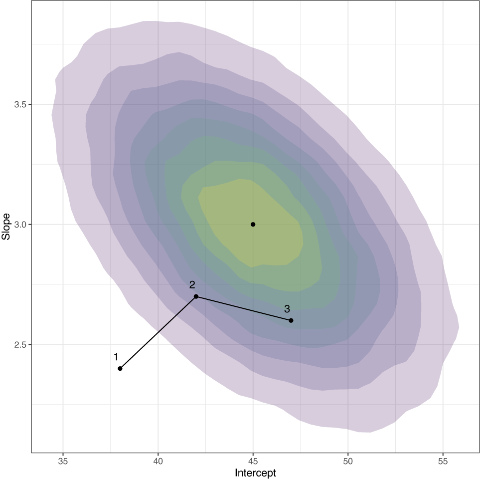



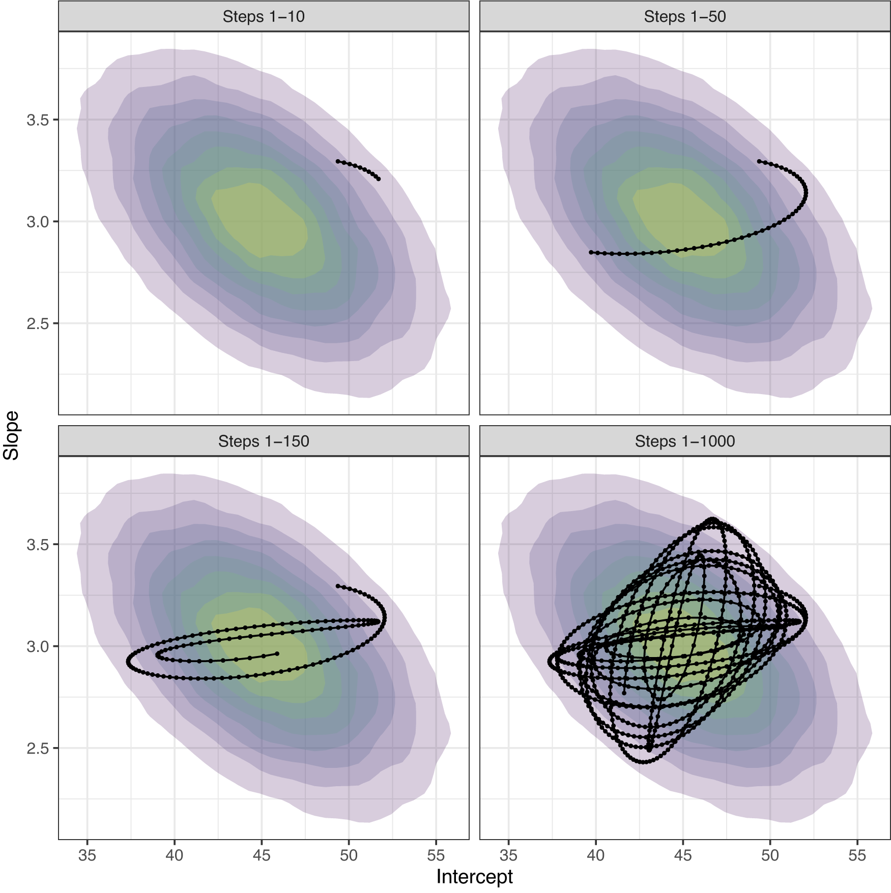

 Open access

