2. The general model

In what follows $x\vee y=\max(x,y)$ , $x\wedge y=\min(x,y)$ , $x^+=x\vee 0$ , and $x^-=({-}x)^+$ . In addition, $\sim$ denotes ‘distributed’ or ‘distributed like’ and $\approx$ denotes ‘asymptotic to’.

Consider a càdlàg Lévy process $X=\{X_t \mid t\ge 0\}$ with $X_0=0$ . Associated with each Lévy process is a triplet $(c,\sigma^2,\nu)$ where $c\in\mathbb{R}$ , $\sigma\ge 0$ , and $\nu$ is a (sigma-finite) measure, called the Lévy measure which satisfies $\nu(\{0\})=0$ , $\int_{\mathbb{R}}\,x^2\wedge 1\,\nu({\mathrm{d}} x)<\infty$ . Any such Lévy process can be decomposed into a sum of independent processes, where one is a Brownian motion (possibly only a drift), another is a compound Poisson process (possibly zero) with jumps in $\mathbb{R}\setminus[-1,1]$ , and, finally, a convergent sum of centered compound Poisson processes of the form $\sum_{n=1}^\infty (X_{n,t}-t\mathrm{E}X_{n,1})$ , where the absolute values of the jumps of the process $X_n$ are in $\left({1}/({n+1}), {1}/{n}\right]$ . For background on Lévy processes and Lévy queues, see, e.g., [Reference Bertoin4, Reference Debicki and Mandjes13, Reference Kella, Perry and Stadje21, Reference Kyprianou25, Reference Sato30].

In addition, let $\tau,\tau_1,\tau_2,\ldots$ be i.i.d. $\exp(\lambda)$ distributed random variables which are also independent of X and use the notation $S_0=0$ and $S_n=\sum_{i=1}^n\tau_i$ for $i\ge 1$ , with renewal counting (Poisson) process $N_t=\sup\{n \mid S_n\le t\}$ . Finally, let $U,U_1,U_2,\ldots$ be i.i.d. with $\mathrm{P}(U\in[0,1])=1$ . These are thought of as random proportions and are independent of all the other random objects defined thus far.

For $t\ge 0$ , denote $L_t=-\inf_{0\le s\le t}X_s$ , $W_t=X_t+L_t$ , and, for $x\ge 0$ ,

(1) \begin{align}L^x_t&=\left({-}\inf_{0\le s\le t}(x+X_s)\right)^+=(L_t-x)^+ , \nonumber\\W^x_t&=x+X_t+L^x_t=X_t+x\vee L_t=W_t+ (x-L_t)^+.\end{align}

This is the reflection (Skorokhod) map associated with $\{x+X_t \mid t\ge 0\}$ where $(L^x_t,W^x_t)$ are the unique càdlàg processes that jointly satisfy (see [Reference Kella17]):

1. (i) $L^x_0=0$ and $L^x_t$ is nondecreasing in t;

2. (ii) $W^x_t\ge 0$ for each $t\ge 0$ ; and

3. (iii) $\{t \mid W^x_t=0\}\subset \{t \mid L^x_s < L^x_t\ \forall s\in [0,t)\}$ .

Now denote $\sigma_sX=\{X_{t+s}-X_s\mid t\ge 0\}$ (which is independent of the history of X until time s) and let $(\sigma_sL^x_t,\sigma_sW^x_t)$ be the corresponding reflection map associated with $\sigma_sX$ . Let $Z=\{Z_t \mid t\ge 0\}$ be defined as follows. Assume that we have already defined it on $[0,S_n)$ . Then for $t\in [S_n,S_{n+1})$ , $Z_t=\sigma_{S_n}W^{U_nZ_{S_n-}}_{t-S_n}$ , where $Z_{t-}=\lim_{v\uparrow t}Z_v$ . Namely, at time $S_n$ , which we refer to as collapse epochs, the content modeled by the process Z collapses to a fraction $U_n$ of its precollapse level and continues according to a reflected Lévy process until the next collapse epoch. Here $Z_0$ may have any distribution and is assumed to be independent of everything else.

Comment 1. In fact, because of the assumptions made until now, Z is a (nonnegative) Markov process with the following generator:

(2) \begin{align}\mathcal{A}g(x) & = cg'(x)+\frac{\sigma^2}{2}g''(x)+\int_{\mathbb{R}}\left(g(x+y)-g(x)-g'(x)y1_{[-1,1]}(y)\right)\nu(\mathrm{d}y)\nonumber\\& \quad +\lambda(\mathrm{E}g(Ux)-g(x))\,\end{align}

for twice continuously differentiable g with $g(x)=g(0)$ for $x\le 0$ (hence, $g'(x)=g''(x)=0$ for $x\le 0$ ). In particular, for $x\le 0$ it may be checked that

(3) \begin{equation}\mathcal{A}g(x)=\int_{({-}x,\infty)}(g(x+y)-g(0))\nu(\mathrm{d}y)=\int_0^\infty g'(y)\nu({-}x+y)\,\mathrm{d}y.\end{equation}

This can be shown by applying the (local) martingales discussed in [Reference Kella and Yor24] or [Reference Kella and Boxma19] but will not be needed for what follows.

A famous result, which in particular may be found in [Reference Bertoin4, Reference Debicki and Mandjes13, Reference Kyprianou25, Reference Sato30], is that $W_\tau$ and $L_\tau$ are independent. By (1) this implies the following decomposition:

(4) \begin{equation} \big(W^x_\tau,L^x_\tau \big)=(W_\tau,0)+ \big((x-L_\tau)^+,(L_\tau-x)^+ \big) ,\end{equation}

where the two random vectors on the right are independent. In particular, denoting $w(\alpha)= \mathrm{E}{\mathrm{e}}^{-\alpha W_\tau}$ , we have that, for $\alpha,\beta\ge 0$ ,

(5) \begin{equation} \mathrm{E}{\mathrm{e}}^{-\alpha W^x_\tau-\beta L^x_\tau}=w(\alpha)\,\mathrm{E}{\mathrm{e}}^{-\alpha (x-L_\tau)^+-\beta (L_\tau-x)^+}.\end{equation}

With our setup, it follows from (4) that

(6) \begin{equation}Z_{S_n-}=\sigma_{S_{n-1}} W_{\tau_n}+ (Z_{S_{n-1}-}U_n-\sigma_{S_{n-1}}L_{\tau_n})^+ ,\end{equation}

where $\sigma_{S_{n-1}} W_{\tau_n},Z_{S_{n-1}-},U_n,\sigma_{S_{n-1}}L_{\tau_n}$ are independent and $\sigma_{S_{n-1}} W_{\tau_n},U_n,\sigma_{S_{n-1}}L_{\tau_n}$ are distributed like $W_\tau,U,L_\tau$ , respectively.

We observe that by PASTA the ergodic distribution of the continuous time process Z is the same as that of the discrete time process $Z_{S_n-}$ and, therefore, it is important to study this latter process. With $\zeta_n=Z_{S_n-}$ , $V_n=\sigma_{S_{n-1}}W_{\tau_n}$ , and $Y_n=\sigma_{S_{n-1}}L_{\tau_n}$ we therefore have the following Lindley-style version of an autoregressive sequence:

(7) \begin{equation}\zeta_n=V_n+(\zeta_{n-1}U_n-Y_n)^+,\end{equation}

where all four random variables on the right are independent with $V_n\sim W_\tau$ , $U_n\sim U$ , and $Y_n\sim L_\tau$ . In the next section we consider this recursion in some detail.

3. Lindley-style autoregressive recursions

Consider the recursion (for now, deterministic),

(8) \begin{equation}z_n=v_n+(z_{n-1}u_n-y_n)^+ , \quad n \geq 1,\end{equation}

where $v_{i-1},y_i\ge 0$ , $u_i\in[0,1]$ for $i\ge 1$ . In addition, let $z_0=v_0$ . This is the same as letting $z_{-1}=0$ , defining $u_0\in[0,1]$ arbitrarily and starting the recursion one index earlier. Furthermore, let $\Pi_0=1$ and $\Pi_n=\prod_{i=1}^n u_i$ for $n\ge 1$ .

We first observe that if $z'_n=v_n+(z_{n-1}'u_n-y_n)^+$ and $z''_n=v_n+(z_{n-1}''u_n-y_n)^+$ , for any two choices where $z''_0\ge z'_0\ge 0$ , then it follows by induction that $z''_n\ge z'_n$ for all $n\ge 0$ . Moreover:

• • when $z''_{n-1}u_n\le y_n$ we have that $z''_n-z'_n=0\le \big(z''_{n-1}-z'_{n-1}\big)u_n$ ;

• • when $z'_{n-1}u_n>y_n$ we have that $z''_n-z'_n=\big(z''_{n-1}-z'_{n-1}\big)u_n$ ;

• • when $z'_{n-1}u_n\le y_n < z''_{n-1}u_n$ we have that

  (9) \begin{equation}z''_n-z'_n=z''_{n-1}u_n-y_n\le z''_{n-1}u_n-y_n+y_n-z'_{n-1}u_n= \big(z''_{n-1}-z'_{n-1} \big) u_n .\end{equation}

Therefore, whenever $z''_0\ge z'_0\ge 0$ , for all $n\ge 1$ , $z''_n-z'_n\le (z''_{n-1}-z'_{n-1})u_n$ and, thus, for every $n\ge 0$ ,

(10) \begin{equation} 0\le z''_n-z'_n\le \big(z''_0-z'_0 \big)\Pi_n .\end{equation}

In particular, this implies the following.

We note that since we will be replacing $u_i$ by i.i.d. random variables $U_i\sim U$ with support in [0, 1], then, unless $\mathrm{P}(U=1)=1$ , it will always hold that $\prod_{i=1}^nU_i\to 0$ as $n\to\infty$ .

We begin by assuming that $u_i>0$ for all $i\ge 1$ , so that $\Pi_n>0$ for all $n\ge1$ . Denoting, for $n\ge 1$ ,

(11) \begin{equation}w_n=\frac{z_n-v_n}{\Pi_n}, \quad x_n=\frac{v_{n-1}}{\Pi_{n-1}}-\frac{y_n}{\Pi_n},\end{equation}

we have that $w_0=0$ and, for $n\ge 1$ , $w_n=(w_{n-1}+x_n)^+$ , which is Lindley’s recursion. Thus, with $s_0=0$ and $s_n=\sum_{i=1}^nx_i$ for $n\ge 1$ we have the well-known solution:

(12) \begin{equation}w_n=s_n-\min_{0\le k\le n}s_k=\max_{0\le k\le n}(s_n-s_{n-k})\end{equation}

and, thus,

(13) \begin{equation}z_n=v_n+\max_{0\le k\le n} ((s_n-s_{n-k})\Pi_n).\end{equation}

For $k=0$ we have that $(s_n-s_{n-k})\Pi_n=0$ whereas for $1\le k\le n$ we have

(14) \begin{align}(s_n-s_{n-k})\Pi_n&=\sum_{i=n-k+1}^n \left(\frac{v_{i-1}}{\Pi_{i-1}}-\frac{y_i}{\Pi_i}\right)\Pi_n\nonumber\\&=\sum_{i=1}^k \left(\frac{v_{n-i}}{\Pi_{n-i}}-\frac{y_{n-i+1}}{\Pi_{n-i+1}}\right)\Pi_n ,\end{align}

recalling that $v_0=0$ (relevant for $i=k=n$ ). Now,

(15) \begin{equation}\frac{\Pi_n}{\Pi_{n-i}}=\prod_{j=n-i+1}^nu_j=\prod_{j=1}^i u_{n-j+1}\end{equation}

and, similarly, for $i=1$ , we have that $\Pi_n/\Pi_{n-1+1}=1$ and for $2\le i\le k\le n$ ,

(16) \begin{equation}\frac{\Pi_n}{\Pi_{n-i+1}}=\prod_{j=n-i+2}^n u_j=\prod_{j=1}^{i-1} u_{n-j+1}.\end{equation}

This implies that we can write

(17) \begin{equation}(s_n-s_{n-k})\Pi_n=\sum_{i=1}^k v_{n-i}\prod_{j=1}^iu_{n-j+1}-\sum_{i=1}^ky_{n-i+1}\prod_{j=1}^{i-1}u_{n-j+1},\end{equation}

where an empty product is defined to be one and an empty sum is zero. Therefore, we finally have that

(18) \begin{equation}z_n=v_n+\max_{0\le k\le n}\left(\sum_{i=1}^k(v_{n-i}u_{n-i+1}-y_{n-i+1})\prod_{j=1}^{i-1}u_{n-j+1}\right) .\end{equation}

We emphasize the fact that for $n=0$ we have that (since empty sums are zero), (18) implies that $z_0=v_0$ as initially assumed. Finally, it is a straightforward exercise to show by induction that (18) holds also for the case where $u_i$ are allowed to be zero. For each such i we have that $z_i=v_i$ and the recursion evidently restarts from that point.

Now, if we replace $\{(v_{i-1},u_i,y_i) \mid i\ge 1\}$ by three independent i.i.d. sequences $\{(V_{i-1},U_i,Y_i) \mid i\ge 1\}$ of nonnegative random variables and $\{z_n \mid n\ge 0\}$ by the random variable $\zeta_n$ , then by taking each of the random vectors $V_0,\ldots,V_n$ , $U_1,\ldots,U_n$ , and $Y_1,\ldots,Y_n$ in reverse order it follows that

(19) \begin{equation}\zeta_n\sim V_0+\max_{0\le k\le n}\left(\sum_{i=1}^k (V_iU_i-Y_i)\prod_{j=1}^{i-1}U_j\right),\end{equation}

where an empty sum is zero and an empty product is one. Therefore, $\zeta_n$ is stochastically increasing and bounded above by $\sum_{i=0}^nV_i\prod_{j=1}^iU_j$ and, hence, if $\mathrm{E}V_0<\infty$ and $\mathrm{P}(U_i=1)<1$ , $\zeta_n$ converges in distribution to an almost surely (a.s.) finite random variable $\zeta$ which is distributed like an independent sum of two random variables. The first is distributed like $V_0$ and the second like

(20) \begin{equation}\sup_{k\ge 0}\left(\sum_{i=1}^k (V_iU_i- Y_i)\prod_{j=1}^{i-1}U_j\right) .\end{equation}

This is a generalization of the setup (hence, the conclusions) considered in [Reference Boxma, Kella and Mandjes6]. See also [Reference Boxma, Löpker, Mandjes and Palmowski8] for a discussion of recursions of the form $W_n=(W_{n-1}U_n+X_n)^+$ .

4. Stability of the Continuous Time Process

An important question is what are the conditions on Z that ensure that there exists a limiting/ergodic/stationary distribution. If $\mathrm{P}(U=1)=1$ then we have a reflected Lévy process, which is well understood and has been discussed many times in the literature and textbooks, and thus we will assume that $\mathrm{P}(U=1)<1$ . Since the collapse epochs occur according to a Poisson process with rate $\lambda$ , it is clear that true collapses (with $U_i<1$ ) occur according to a Poisson process with rate $\lambda \mathrm{P}(U<1)$ . Therefore, without loss of generality (w.l.o.g.), let us assume that $\mathrm{P}(U=1)=0$ . If $\mathrm{P}(U=0)>0$ then after a geometrically distributed number of trials the process jumps to zero (often called clearing), which implies that it is regenerative and therefore a proper limiting ergodic distribution clearly exists. It remains to consider the case $\mathrm{P}(U=0)=\mathrm{P}(U=1)=0$ . In this case it is clear that $\prod_{i=1}^\infty U_i=0$ a.s.

It is easy to check that if $x\le y$ then $W^x_t\le W^y_t$ for all $t\ge 0$ and that $W^y_t-W^x_t$ is nonincreasing in t. See [Reference Kella and Whitt23] for results like this in the multidimensional setting. Therefore, setting $Z^x$ to be the process Z when started from $Z_0=x$ we have that

(21) \begin{equation}Z_{\tau_1}^y-Z_{\tau_1}^x= \big(W_{\tau_1-}^y-W_{\tau_1-}^x \big)U_1\le (y-x)U_1,\end{equation}

where the left-hand side is nonnegative. Hence, by induction it also follows that

(22) \begin{equation}0\le Z_{S_n}^y-Z_{S_n}^x\le (y-x)\prod_{i=1}^n U_i,\end{equation}

where the right-hand side vanishes a.s. as $n\to\infty$ . Therefore, we also have that

(23) \begin{equation}0\le Z^y_t-Z^x_t\le (y-x)\prod_{i=1}^{N_t}U_i\end{equation}

which vanishes a.s. as $t\to\infty$ . Therefore, it follows that if a limiting distribution exists, it does not depend on the initial distribution of $Z_0$ .

Since $W^x_t=X_t+L_t\vee x\le x+X_t+L_t=x+W_t$ it follows that $Z_{S_n}$ is stochastically bounded by $x\prod_{i=1}^nU_i+\sum_{i=1}^n V_i\prod_{j=i}^nU_j$ where all the variables on the right-hand side are independent and $V_i\sim W_\tau$ . By results from [Reference Kella18] this implies that $\{Z_{S_n} \mid n\ge 0\}$ and, hence, $\{Z_t \mid t\ge 0\}$ are bounded above by a process that has a stationary version. Therefore, tightness of these processes is assured. It also implies that $\{Z_t \mid t\ge 0\}$ has a stationary version by following the (Loynes-type) construction from [Reference Kella18] which is applied there to the case where W is nondecreasing.

Therefore, we can apply PASTA to conclude that the (unique) ergodic distribution of Z is the same as that of the discrete time process $\zeta_n=Z_{S_n-}$ , where we recall $\zeta_n,\zeta$ from Sections 2 and 3. With $Z^*=\zeta$ having the steady-state distribution of $\zeta_n$ (and, hence, also of the process Z), we have that

(24) \begin{equation}Z^*\sim W^{Z^*U}_\tau\sim W_\tau+(Z^*U-L_\tau)^+,\end{equation}

where $Z^*,W_\tau,U,L_\tau$ on the right are independent. To summarize, all that is needed for stability and independence of initial conditions for the continuous time process is that $\mathrm{P}(U_1=1)<1$ and that $\mathrm{E}W_\tau<\infty$ , for which it suffices that $\int_{(1,\infty)}x\nu({\mathrm{d}} x)<\infty$ .

5. The case where X is spectrally positive

When X is spectrally positive, that is, $\nu({-}\infty,0]=0$ , then with

(25) \begin{equation}\varphi(\alpha)=\log \mathrm{E}{\mathrm{e}}^{-\alpha X_1}=-c\alpha+\frac{\sigma^2}{2}\alpha^2+\int_{(0,\infty)}\left({\mathrm{e}}^{-\alpha x}-1+\alpha x1_{(0,1]}(x)\right)\,\nu({\mathrm{d}} x) ,\end{equation}

it may be concluded (e.g. applying the martingale from [Reference Kella and Whitt22], as is done in [Reference Asmussen3, Theorem 3.10, p. 259]) that if X is not a subordinator and $\alpha_\lambda$ is the unique positive root of $\varphi(\alpha)=\lambda$ , then $L_\tau\sim \exp(\alpha_\lambda)$ and

(26) \begin{equation}w(\alpha)=\mathrm{E}{\mathrm{e}}^{-\alpha W_\tau}=\frac{1-\frac{\alpha}{\alpha_\lambda}}{1-\frac{\varphi(\alpha)}{\lambda}}.\end{equation}

Therefore, it follows either by [Reference Asmussen3, Theorem 3.10, p. 259] or from (5) here that, for $\alpha\not=\alpha_\lambda$ ,

(27) \begin{equation}\mathrm{E}{\mathrm{e}}^{-\alpha W^x_\tau-\beta L^x_\tau}=w(\alpha)\,\frac{{\mathrm{e}}^{-\alpha x}-\frac{\alpha+\beta}{\alpha_\lambda+\beta}{\mathrm{e}}^{-\alpha_\lambda x}}{1-\frac{\alpha}{\alpha_\lambda}},\end{equation}

whereas by l’Hôpital’s rule and continuity, for $\alpha=\alpha_\lambda$ the right-hand side is

(28) \begin{equation}\frac{x+\frac{1}{\alpha_\lambda+\beta}}{\varphi'(\alpha_\lambda)} \lambda {\mathrm{e}}^{-\alpha_\lambda x} .\end{equation}

In particular, for $\alpha\not=\alpha_\lambda$ ,

(29) \begin{equation}\mathrm{E}{\mathrm{e}}^{-\alpha W^x_\tau}=w(\alpha) \frac{{\mathrm{e}}^{-\alpha x}-\frac{\alpha}{\alpha_\lambda}{\mathrm{e}}^{-\alpha_\lambda x}}{1-\frac{\alpha}{\alpha_\lambda}}=\frac{{\mathrm{e}}^{-\alpha x}-\frac{\alpha}{\alpha_\lambda}{\mathrm{e}}^{-\alpha_\lambda x}}{1-\frac{\varphi(\alpha)}{\lambda}},\end{equation}

where the term to the right of $w(\alpha)$ is the LST of $(x-L_\tau)^+$ . The case where X is a subordinator is analyzed in [Reference Boxma, Kella and Perry7, Reference Kella18] and is thus ignored here.

From (24) and (29) it therefore follows that if we set $f(\alpha)=\mathrm{E}{\mathrm{e}}^{-\alpha Z^*}$ then

(30) \begin{equation}f(\alpha)=\frac{\mathrm{E}f(\alpha U)-\frac{\alpha}{\alpha_\lambda} \mathrm{E}f(\alpha_\lambda U)}{1-\frac{\varphi(\alpha)}{\lambda}}.\end{equation}

Noting that for $n\ge 1$ we have, with $\delta_{1n}=0$ for $n\ge 2$ and $\delta_{11}=1$ , that

(31) \begin{align} \left(1-\frac{\varphi(\alpha)}{\lambda}\right)f^{(n)}(\alpha)-\frac{1}{\lambda}\,\sum_{k=0}^{n-1} \left(\begin{array}{l}n \\k \end{array}\right) f^{(k)}(\alpha)\varphi^{(n-k)}(\alpha)=\mathrm{E}U^{{nf}^{{(n)}}}(\alpha U)-\frac{\mathrm{E}f(\alpha_{\lambda U})} {\alpha_{\lambda} }\delta_{1n}\end{align}

from which the following recursion is immediate, once we argue that $\mathrm{E}(Z^*)^n<\infty$ whenever $\varphi^{(n)}(0)$ is finite.

Lemma 2. Assume that $\mathrm{P}(U=1)<1$ and for $n\ge 0$ denote $m_n=\mathrm{E}(Z^*)^n=({-}1)^nf^{(n)}(0)$ , and

(32) \begin{equation}c_n=({-}1)^n\varphi^{(n)}(0)= \begin{cases} 0&n=0\,\\[4pt]c+\int_{(1,\infty)}x\nu({\mathrm{d}} x)&n=1\,\\[4pt]\sigma^2+\int_{(0,\infty)}x^2\nu({\mathrm{d}} x)&n=2\,\\[4pt]\int_{(0,\infty)}x^n\nu({\mathrm{d}} x)&n\ge 3. \end{cases} \end{equation}

Then, for all $n\ge 0$ , $m_n<\infty$ when $c_n<\infty$ and for $n\ge 2$

(33) \begin{equation} m_n=\frac{1}{1-\mathrm{E}U^n}\,\frac{1}{\lambda}\,\sum_{k=0}^{n-1} \left(\begin{array}{l}n\\k \end{array} \right)m_kc_{n-k}, \end{equation}

where $m_0=1$ and

(34) \begin{equation} m_1=\frac{1}{1-\mathrm{E}U}\left(\frac{c_1}{\lambda}+\frac{\mathrm{E}f(\alpha_\lambda U)}{\alpha_\lambda}\right). \end{equation}

Proof. Since (33) and (34) are obtained by letting $\alpha\downarrow 0$ in (31) and rearranging terms, provided that all the terms are finite, it remains to show that when $c_n<\infty$ then $m_n<\infty$ , hence $c_k,m_k<\infty$ for $k\le n$ . Recall (19) which implies that $\zeta_n$ is stochastically bounded by the process $V_0+\sum_{i=1}^n V_i\prod_{j=1}^iU_j$ and, thus, $Z^*\le_{\text{st}} V_0+\sum_{i=1}^\infty V_i\prod_{j=1}^iU_j$ , where in this case $V_i\sim\mathrm{W}_\tau$ . One may apply Minkowski’s inequality to argue that if $\mathrm{E}V_0^n=\mathrm{E}W_\tau^n<\infty$ then

(35) \begin{equation} \|V_0+\sum_{i=1}^n V_i\prod_{j=1}^iU_j\|_n\le \|V_0\|_n\sum_{i=0}^n\|U_1\|_n^i\le\frac{\|V_0\|}{1-\|U\|_n}, \end{equation}

where $\|Y\|_n=(\mathrm{E}|Y|^n)^{ 1/n}$ , so that by monotone convergence we also have that $\mathrm{E}(V_0+\sum_{i=1}^\infty V_i\prod_{j=1}^iU_j)^n<\infty$ and, thus, $\mathrm{E}(Z^*)^n<\infty$ . To see that $\mathrm{E}W_\tau^n<\infty$ whenever $c_n<\infty$ we recall that $X_\tau=W_\tau-L_\tau$ where $W_\tau,L_\tau$ are independent and $L_\tau\sim\exp(\alpha_\lambda)$ has moments of all orders. Since whenever $c_n<\infty$ , $\mathrm{E}X_t^n$ is a polynomial in t of order at most n, which is easy to check by first computing factorial moments via $\log \mathrm{E}{\mathrm{e}}^{-\alpha X_t}=\varphi(\alpha)t$ , and since $\tau\sim\exp(\lambda)$ has finite moments of all orders, then $\mathrm{E}X^n_\tau<\infty$ and therefore necessarily also $\mathrm{E}W_\tau^n<\infty$ , which completes the argument.

It turns out that when $U\sim\text{Uniform}(0,1)$ the problem of identifying $\mathrm{E}{\mathrm{e}}^{-\alpha Z^*}$ for all $\alpha\ge 0$ (in particular, $\mathrm{E}f(\alpha_\lambda U)/\alpha_\lambda$ ), becomes tractable. For this case $\mathrm{E}U^n=(n+1)^{-1}$ .

Theorem 1. Assume that $U\sim\text{Uniform}(0,1)$ and that X is a finite mean spectrally positive Lévy process, which is not a subordinator. Then, with

(36) \begin{equation} b=\left(\int_0^{\alpha_\lambda} {\mathrm{e}}^{-\int_0^x\frac{\varphi(y)}{y(\lambda-\varphi(y))}\,{\mathrm{d}} y}\,{\mathrm{d}} x\right)^{-1}, \end{equation}

we have that

(37) \begin{equation} f(\alpha)=\mathrm{E}{\mathrm{e}}^{-\alpha Z^*}=\begin{cases}\frac{b}{1-\frac{\varphi(\alpha)}{\lambda}}\,\int_\alpha^{\alpha_\lambda} {\mathrm{e}}^{-\int_\alpha^x\frac{\varphi(y)}{y(\lambda-\varphi(y))}\,{\mathrm{d}} y}\,{\mathrm{d}} x, &\alpha\in[0,\alpha_\lambda),\\ \\ \frac{b}{\frac{1}{\alpha_\lambda}+\frac{\varphi'(\alpha_\lambda)}{\lambda}},&\alpha=\alpha_\lambda,\\ \\ \frac{b}{\frac{\varphi(\alpha)}{\lambda}-1}\,\int_{\alpha_\lambda}^\alpha {\mathrm{e}}^{-\int_x^\alpha\frac{\varphi(y)}{y(\varphi(y)-\lambda)}\,{\mathrm{d}} y}\,{\mathrm{d}} x,&\alpha\in(\alpha_\lambda,\infty). \end{cases}\end{equation}

Moreover, whenever $X_t=J_t-dt$ where J is a nonzero pure jump subordinator and $d>0$ then $\mathrm{P}(Z^*=0)= {\lambda b}/{2d}$ . In all other cases $\mathrm{P}(Z^*=0)=0$ .

Proof. We first note that when $U\sim\text{Uniform}(0,1)$ then with $F(\alpha)=\int_0^\alpha f(x)dx$ , $b=2F(\alpha_\lambda)/\alpha_\lambda^2$ and $a(\alpha)=\left(\alpha\left(1-\frac{\varphi(\alpha)}{\lambda}\right)\right)^{-1}$ , (30) becomes

(38) \begin{equation} f(\alpha)=F'(\alpha)=\frac{F(\alpha)-\frac{\alpha^2}{2}b}{\alpha\left(1-\frac{\varphi(\alpha)}{\lambda}\right)} =a(\alpha)F(\alpha)-\frac{\alpha^2}{2}a(\alpha)b. \end{equation}

From this it immediately follows via L’Hôpital’s rule on the right-hand side and the fact that $\varphi(\alpha_\lambda)=\lambda$ , that

(39) \begin{equation} f(\alpha_\lambda)=\frac{f(\alpha_\lambda)-\alpha_\lambda b}{-\alpha_\lambda\frac{\varphi'(\alpha_\lambda)}{\lambda}}, \end{equation}

so that the case $\alpha=\alpha_\lambda$ in (37) is immediate.

From (38) it now follows that, for $0<\alpha<\beta<\alpha_\lambda$ and for $\alpha_\lambda < \alpha < \beta$ ,

(40) \begin{equation}F(\beta){\mathrm{e}}^{-\int_\alpha^\beta a(y)\,{\mathrm{d}} y}=F(\alpha)-b\int_\alpha^\beta \frac{x^2}{2}a(x){\mathrm{e}}^{-\int_\alpha^xa(y)\,{\mathrm{d}} y}\,{\mathrm{d}} x.\end{equation}

Integration by parts gives

(41) \begin{equation}\int_\alpha^\beta \frac{x^2}{2}a(x){\mathrm{e}}^{-\int_\alpha^xa(y)\,{\mathrm{d}} y}\,{\mathrm{d}} x=\frac{\alpha^2}{2}-\frac{\beta^2}{2} {\mathrm{e}}^{-\int_\alpha^\beta a(y)\,{\mathrm{d}} y}+\int_\alpha^\beta x{\mathrm{e}}^{-\int_\alpha^x a(y)\,{\mathrm{d}} y}\,{\mathrm{d}} x.\end{equation}

Since for a sufficiently small neighborhood of $\alpha_\lambda$ we have that

(42) \begin{equation}\frac{\varphi(\alpha)-\lambda}{\alpha-\alpha_\lambda}\in (\varphi'(\alpha_\lambda)-\epsilon,\varphi'(\alpha_\lambda)+\epsilon),\end{equation}

where $0<\epsilon<\varphi'(\alpha_\lambda)$ and $\varphi'(\alpha_\lambda)$ is finite and positive, then for every $\alpha\in (0,\alpha_\lambda)$ we necessarily have that $\int_\alpha^{\alpha_\lambda}a(x)\,{\mathrm{d}} x=\infty$ . Therefore, letting $\beta\uparrow\alpha_\lambda$ in (40), implies that

(43) \begin{equation}F(\alpha)=b\left( \frac{\alpha^2}{2}+\int_\alpha^{\alpha_\lambda}x{\mathrm{e}}^{-\int_\alpha^{x}a(y)\,{\mathrm{d}} y}\,{\mathrm{d}} x\right).\end{equation}

Differentiating both sides leads to

(44) \begin{equation}f(\alpha)= \mathrm{E}{\mathrm{e}}^{-\alpha Z^*}=b a(\alpha)\int_\alpha^{\alpha_\lambda}x{\mathrm{e}}^{-\int_\alpha^{x}a(y)\,{\mathrm{d}} y}\,{\mathrm{d}} x .\end{equation}

We now recall that $a(\alpha)=(\alpha (1-\varphi(\alpha)/\lambda))^{-1}$ and note that for $\alpha < x < \alpha_\lambda$ we have that $x/\alpha={\mathrm{e}}^{\int_\alpha^x {y}^{-1}\,{\mathrm{d}} y}$ , implying that

(45) \begin{equation}a(\alpha)x{\mathrm{e}}^{-\int_\alpha^x a(y)\,{\mathrm{d}} y}=\frac{1}{1-\frac{\varphi(\alpha)}{\lambda}}\, {\mathrm{e}}^{\int_\alpha^x \left(\frac{1}{y}-a(y)\right)\,{\mathrm{d}} y}=\frac{1}{1-\frac{\varphi(\alpha)}{\lambda}}\,{\mathrm{e}}^{-\int_\alpha^x \frac{\varphi(y)}{y(\lambda-\varphi(y))}\,{\mathrm{d}} y},\end{equation}

so that together with (44), the case $\alpha\in [0,\alpha_\lambda)$ in (37) follows.

Recalling, by assumption, that $\varphi'(0)=-\mathrm{E}X_1$ is finite then $\int_0^x \frac{\varphi(y)}{y(\lambda-\varphi(y))}\,{\mathrm{d}} y$ is convergent for any $x\in (0,\alpha_\lambda)$ so that, since $\varphi(\alpha)\to 0$ as $\alpha\downarrow 0$ , we finally obtain (36).

For the case $\alpha>\alpha_\lambda$ we observe that in (40) we can multiply both sides by ${\mathrm{e}}^{\int_\alpha^\beta a(y)\,{\mathrm{d}} y}$ and note that for $y>\alpha_\lambda$

(46) \begin{equation} a(y)=\frac{1}{y\left(1-\frac{\varphi(y)}{\lambda}\right)}=-\frac{1}{y\left(\frac{\varphi(y)}{\lambda}-1\right)}.\end{equation}

The rest is a repetition of the proof for the case $\alpha\in[0,\alpha_\lambda)$ , where eventually we let $\alpha\downarrow \alpha_\lambda$ and replace $\beta$ in the resulting expression by $\alpha$ .

We finally turn to $\mathrm{P}(Z^*=0)$ . Note that

(47) \begin{equation} \int_{\alpha_\lambda}^\alpha {\mathrm{e}}^{-\int_x^\alpha \frac{\varphi(y)}{y(\varphi(y)-\lambda)}\,{\mathrm{d}} y}\,{\mathrm{d}} x = \alpha\int_{\alpha_\lambda/\alpha}^1 {\mathrm{e}}^{-\int_x^1 \frac{\varphi(\alpha y)}{y(\varphi(\alpha y)-\lambda)}\,{\mathrm{d}} y}\,{\mathrm{d}} x,\end{equation}

and that by bounded convergence

(48) \begin{equation} \lim_{\alpha\to\infty}\int_{\alpha_\lambda/\alpha}^1 {\mathrm{e}}^{-\int_x^1 \frac{\varphi(\alpha y)}{y(\varphi(\alpha y)-\lambda)}\,{\mathrm{d}} y}\,{\mathrm{d}} x=\int_0^1{\mathrm{e}}^{-\int_x^1\frac{1}{y}\,{\mathrm{d}} y}\,{\mathrm{d}} x=\int_0^1x\,{\mathrm{d}} x=\frac{1}{2}. \end{equation}

Therefore,

(49) \begin{equation} \mathrm{P}(Z^*=0)=\frac{b}{2}\lim_{\alpha\to\infty}\frac{\alpha}{\frac{\varphi(\alpha)}{\lambda}-1}=\frac{\lambda b}{2}\,\lim_{\alpha\to\infty}\frac{\alpha}{\varphi(\alpha)}.\end{equation}

If our Lévy process is a subordinator minus a positive drift d then

(50) \begin{equation} \varphi(\alpha)=d\alpha-\int_{(0,\infty)}\left(1-{\mathrm{e}}^{-\alpha x}\right)\nu({\mathrm{d}} x)=\alpha\left(d-\int_0^\infty {\mathrm{e}}^{-\alpha x}\nu(x,\infty)\,{\mathrm{d}} x\right).\end{equation}

In this case the mean is finite if and only if $\int_0^\infty \nu(x,\infty)\,{\mathrm{d}} x=\int_{(0,\infty)}x\nu({\mathrm{d}} x)<\infty$ , in which case (bounded convergence) $\int_0^\infty {\mathrm{e}}^{-\alpha x}\nu(x,\infty)\,{\mathrm{d}} x$ vanishes, whence, $\varphi(\alpha)/\alpha\to d$ as $\alpha\to\infty$ .

In all other cases (recalling that X is not a subordinator), that is, when there is a Brownian motion part or $\int_{(0,1]}x\nu({\mathrm{d}} x)=\infty$ (that is, an unbounded variation component) we have that $\varphi(\alpha)/\alpha\to \infty$ as $\alpha\to\infty$ , hence the right-hand side of (49) is zero.

Remark 2. It is easy to check that for $\alpha\in[0,\alpha_\lambda)$ and with

(51) \begin{equation} g(\alpha)\,:\!=\,\int_0^{\alpha} {\mathrm{e}}^{-\int_0^x \frac{\varphi(y)}{y(\lambda-\varphi(y))}\,{\mathrm{d}} y}\,{\mathrm{d}} x,\end{equation}

we have the following representation (when $U\sim\text{Uniform}(0,1)$ ).

(52) \begin{align} f(\alpha)=\mathrm{E}{\mathrm{e}}^{-\alpha Z^*}=\frac{1-\frac{g(\alpha)}{g(\alpha_\lambda)}}{g'(\alpha)\left(1-\frac{\varphi(\alpha)}{\lambda}\right)}.\end{align}

Consequently, from (24) and (26) it follows that

(53) \begin{equation} \mathrm{E}{\mathrm{e}}^{-\alpha (Z^*U-L_\tau)^+}=\frac{1-\frac{g(\alpha)}{g(\alpha_\lambda)}}{g'(\alpha)\left(1-\frac{\alpha}{\alpha_\lambda}\right)}.\end{equation}

We complete this remark by emphasizing that $b=1/g(\alpha_\lambda)$ .

6. Examples and Tail Behavior

In this section we work out the LST of $Z^*$ , and hence of Z, for the two cases of reflected Brownian motion with collapse (Section 6.1) and the $M/M/1$ queue with collapse (Section 6.2). In both cases, collapses occur according to a Poisson process with rate $\lambda$ , and instantaneously remove a Uniform(0,1) distributed fraction of the workload present. In these two examples we use the notation g and the expression for f from Remark 2. We conclude in Section 6.3 with a discussion about the tail behavior of $Z^*$ for the compound Poisson case with a negative drift.

6.1. Reflected Brownian motion with collapse

The Laplace exponent of Brownian motion with drift c is given by (cf. (25))

(54) \begin{equation}\varphi(\alpha) = -c\alpha + \frac{\sigma^2}{2} \alpha^2 .\end{equation}

In order to obtain the LST $f(\alpha)$ of the steady-state level of the reflected Brownian motion with collapses, we need to determine $g(\alpha)$ and its derivative, which feature in (52). First write

(55) \begin{equation} - \frac{\varphi(y)}{y(\lambda - \varphi(y))} = \frac{c - \frac{\sigma^2}{2} y}{\lambda +cy - \frac{\sigma^2}{2} y^2} = \frac{y-\frac{2c}{\sigma^2}}{(y-y_1)(y-y_2)} , \end{equation}

where

(56) \begin{equation} y_{1,2} = \frac{c}{\sigma^2} \pm \sqrt{\frac{c^2}{\sigma^4} + \frac{2\lambda}{\sigma^2}} . \end{equation}

It is easily verified that $y_1>0$ and $y_2<0$ , with 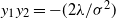$y_1y_2 = -({2\lambda}/{\sigma^2})$ and $y_1+y_2 = {2c}/{\sigma^2}$ ; and of course $y_1 = \alpha_\lambda$ , the unique positive zero of $\lambda - \varphi(\alpha)$ .

Using a partial fraction expansion, we can rewrite (55) as follows:

(57) \begin{equation} - \frac{\varphi(y)}{y(\lambda-\varphi(y))} \,=\, \frac{D_1}{y-y_1} + \frac{D_2}{y-y_2} , \end{equation}

where

(58) \begin{equation} D_1 = \frac{-y_2}{y_1-y_2} > 0, \quad D_2 = \frac{y_1}{y_1-y_2} > 0. \end{equation}

It is now easily verified that

(59) \begin{equation} g(\alpha) =\int_0^\alpha \left(\frac{x-y_1}{-y_1}\right)^{D_1} \left(\frac{x-y_2}{-y_2}\right)^{D_2} \,{\mathrm{d}} x , \end{equation}

and, hence,

(60) \begin{equation} \frac{g(\alpha)}{g(\alpha_\lambda)} = \frac{g(\alpha)}{g(y_1)} = \frac{\int_0^\alpha (x-y_1)^{D_1} (x-y_2)^{D_2} \,{\mathrm{d}} x}{\int_0^{y_1} (x-y_1)^{D_1} (x-y_2)^{D_2} \,{\mathrm{d}} x} , \end{equation}

while

(61) \begin{equation} g'(\alpha) = \left(\frac{\alpha -y_1}{-y_1}\right)^{D_1} \left(\frac{\alpha -y_2}{-y_2}\right)^{D_2} . \end{equation}

Substitution in (52) shows that the LST of the steady-state level of our reflected Brownian motion with collapse is, for $\alpha \in [0,y_1)$ , given by

(62) \begin{align} f(\alpha) &= \frac{y_1y_2}{(\alpha-y_1)(\alpha-y_2)} \left(\frac{\alpha -y_1}{-y_1}\right)^{-D_1} \left(\frac{\alpha -y_2}{-y_2}\right)^{-D_2} \nonumber \\ \nonumber\\ &\qquad \times \left(1 - \frac{\int_0^\alpha (x-y_1)^{D_1} (x-y_2)^{D_2} \,{\mathrm{d}} x}{\int_0^{y_1} (x-y_1)^{D_1} (x-y_2)^{D_2} \,{\mathrm{d}} x} \right) \\ \nonumber\\ &= \left(\frac{y_1}{y_1 - \alpha}\right)^{1+D_1} \left(\frac{-y_2}{-y_2 + \alpha}\right)^{1+D_2} \left(1 -\frac{\int_0^\alpha (x-y_1)^{D_1} (x-y_2)^{D_2} \,{\mathrm{d}} x}{\int_0^{y_1} (x-y_1)^{D_1} (x-y_2)^{D_2} \,{\mathrm{d}} x} \right) . \nonumber \end{align}

Note that the first two terms in the last line of (62) represent the LST of the difference of two independent Gamma distributed random variables.

Remark 5. It should be observed that $g(\alpha)$ can be expressed in incomplete beta functions. The incomplete beta function $B(z;\,a_1,a_2)$ is defined as (e.g. [Reference Abramowitz and Stegun1, p.263])

(63) \begin{equation} B(z;\,a_1,a_2) \,:\!=\, \int_0^z t^{a_1-1} (1-t)^{a_2-1} \,{\mathrm{d}} t ; \end{equation}

it can also be expressed as a hypergeometric function via the identity

(64) \begin{equation} B(z;\,a_1,a_2) = \frac{z^{a_1}}{a_1} {}_2F_1(a_1,1-a_2;\,a_1+1;\,z) . \end{equation}

The transformation $t\,:\!=\, ({x-y_2})/({y_1-y_2})$ gives

(65) \begin{eqnarray} && \int_0^\alpha (x-y_1)^{D_1} (x-y_2)^{D_2} \,{\mathrm{d}} x = ({-}1)^{D_1} (y_1-y_2)^{D_1+D_2+1} \,\int_{\frac{-y_2}{y_1-y_2}}^{\frac{\alpha-y_2}{y_1-y_2}} t^{D_2}(1-t)^{D_1} \,{\mathrm{d}} t \nonumber\\&=& ({-}1)^{D_1} (y_1-y_2)^2 \left[B\left(\frac{\alpha-y_2}{y_1-y_2};\,1+D_2,1+D_1\right) - B\left(\frac{-y_2}{y_1-y_2};\,1+D_2,1+D_1\right) \right]. \nonumber\\ \end{eqnarray}

6.2. The $M/M/1$ queue with collapse

A second example in which one can explicitly determine the LST of the steady-state reflected spectrally positive Lévy process with collapse concerns the workload in an $M/M/1$ queue with collapse. Denote the arrival rate of customers by $\gamma$ and the service rate by $\mu$ ; the server works at speed d workload units per time unit. Collapses again occur according to a Poisson process with rate $\lambda$ , and remove (and maintain) a Uniform(0,1) distributed part of the workload present.

The Laplace exponent of the workload process in an $M/M/1$ queue is given by

(66) \begin{equation} \varphi(\alpha) = d \alpha - \gamma \frac{\alpha}{\mu+\alpha} . \end{equation}

Very similar to the previous subsection, we can write

(67) \begin{equation} - \frac{\varphi(y)}{y(\lambda - \varphi(y))} =\frac{y+\mu - \frac{\gamma}{d}}{(y-z_1)(y-z_2)},\end{equation}

where

(68) \begin{equation} z_{1,2} = \frac{1}{2} \left[ \frac{\lambda+\gamma}{d} - \mu \pm \sqrt{\left(\frac{\lambda+\gamma}{d}-\mu\right)^2 + 4 \frac{\lambda\mu}{d} } \right].\end{equation}

It is easily verified that $z_1>0$ and $z_2<0$ , with $z_1z_2 = - ({\lambda \mu}/{d})$ and $z_1+z_2= ({\lambda+\gamma})/{d}-\mu$ ; and of course $z_1=\alpha_\lambda$ , the unique positive zero of $\lambda - \varphi(\alpha)$ .

Using a partial fraction expansion, we can rewrite (67) as follows:

(69) \begin{equation} - \frac{\varphi(y)}{y(\lambda - \varphi(y))} =\frac{F_1}{y-z_1} + \frac{F_2}{y-z_2},\end{equation}

where

(70) \begin{equation} F_1 = \frac{\frac{\lambda}{d}-z_2}{z_1-z_2} > 0, \quad F_2 = \frac{z_1 - \frac{\lambda}{d}}{z_1-z_2} >0.\end{equation}

It is now easily verified that

(71) \begin{equation} g(\alpha) = \int_0^\alpha \left(\frac{x-z_1}{-z_1}\right)^{F_1} \left(\frac{x-z_2}{-z_2}\right)^{F_2} \,{\mathrm{d}} x , \end{equation}

and, hence,

(72) \begin{equation} \frac{g(\alpha)}{g(\alpha_\lambda)} = \frac{g(\alpha)}{g(z_1)} = \frac{\int_0^\alpha (x-z_1)^{F_1} (x-z_2)^{F_2} \,{\mathrm{d}} x}{\int_0^{z_1} (x-z_1)^{F_1} (x-z_2)^{F_2} \,{\mathrm{d}} x} , \end{equation}

while

(73) \begin{equation} g'(\alpha) = \left(\frac{\alpha -z_1}{-z_1}\right)^{F_1} \left(\frac{\alpha -z_2}{-z_2}\right)^{F_2} . \end{equation}

Substitution in (52) shows that the LST of the steady-state workload in the $M/M/1$ queue with collapse is, for $\alpha \in [0,z_1)$ , given by

(74) \begin{align} f(\alpha) &= \frac{z_1z_2}{(\alpha-z_1)(\alpha-z_2)} \left(\frac{\alpha -z_1}{-z_1}\right)^{-F_1} \left(\frac{\alpha -z_2}{-z_2}\right)^{-F_2} \nonumber \\ \nonumber \\ &\qquad\times \,\left(1 - \frac{\int_0^\alpha (x-z_1)^{F_1} (x-z_2)^{F_2} \,{\mathrm{d}} x}{\int_0^{z_1} (x-z_1)^{F_1} (x-z_2)^{F_2} \,{\mathrm{d}} x} \right) \\ \nonumber\\ &= \left(\frac{z_1}{z_1 - \alpha}\right)^{1+F_1} \left(\frac{-z_2}{-z_2 + \alpha}\right)^{1+F_2} \left(1 -\frac{\int_0^\alpha (x-z_1)^{F_1} (x-z_2)^{F_2} \,{\mathrm{d}} x}{\int_0^{z_1} (x-z_1)^{F_1} (x-z_2)^{F_2} \,{\mathrm{d}} x} \right) . \nonumber \end{align}

Just as in Remark 5, one can express this LST in terms of incomplete beta functions. Furthermore, the first two terms in the last line of (74) represent the LST of the difference of two independent Gamma distributed random variables.

Remark 6. We briefly indicate another approach that basically leads to the same first-order inhomogeneous differential equation as (38). The steady-state workload distribution has an atom $p_0$ at zero and conjecture that it is absolutely continuous on $(0,\infty)$ with density $h({\cdot})$ , so that $\mathrm{P}(Z^*\le t)=p_0+\int_0^t h(s)\,{\mathrm{d}} s$ . Level crossing arguments lead to the following equation:

(75) \begin{equation}d h(x)+ \lambda \int_x^\infty h(y) \frac{x}{y}\,{\mathrm{d}} y= \gamma \int_0^x {\mathrm{e}}^{-\mu(x-y)}\,{\mathrm{d}} \mathrm{P}(Z^* < y) .\end{equation}

Here the first term in the left-hand side corresponds to downcrossings of level x due to serving, and the second term in the left-hand side reflects downward jumps due to a uniform collapse with rate $\lambda$ . The term in the right-hand side corresponds to a jump through level x due to a customer arrival: either a jump from zero or from some level $y \in (0,x)$ . Multiplying both sides of (75) by ${\mathrm{e}}^{-\alpha x}$ and integrating from zero to infinity yields, with $f(\alpha) = \mathrm{E}{\mathrm{e}}^{-\alpha Z^*} = p_0 + \int_0^\infty {\mathrm{e}}^{-\alpha x} h(x) \,{\mathrm{d}} x$ :

(76) \begin{equation}d (f(\alpha) -p_0) + \lambda \int_{y=0}^\infty \frac{h(y)}{y} \int_{x=0}^y x {\mathrm{e}}^{-\alpha x} \,{\mathrm{d}} x \,{\mathrm{d}} y = \frac{\gamma}{\mu+\alpha} f(\alpha) .\end{equation}

The second term in the left-hand side can be rewritten as

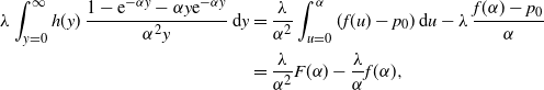(77) \begin{align} \lambda \int_{y=0}^\infty h(y)\, \frac{1 - {\mathrm{e}}^{-\alpha y} -\alpha y {\mathrm{e}}^{-\alpha y}}{\alpha^2 y} \,{\mathrm{d}} y &= \frac{\lambda}{\alpha^2} \int_{u=0}^\alpha (f(u)-p_0) \,{\mathrm{d}} u - \lambda\, \frac{f(\alpha)-p_0}{\alpha}\nonumber\\ &= \frac{\lambda}{\alpha^2} F(\alpha) - \frac{\lambda}{\alpha} f(\alpha) ,\end{align}

where $F(\alpha) = \int_0^\alpha f(x) \,{\mathrm{d}} x$ , cf. above (38), and, hence, we have

(78) \begin{equation} F'(\alpha) \left(\frac{\lambda}{\alpha} -d + \frac{\gamma}{\mu+\alpha}\right) = \frac{\lambda}{\alpha^2} F(\alpha) - d p_0 . \end{equation}

Dividing both sides by ${\lambda}/{\alpha} -d + {\gamma}/({\mu+\alpha})$ results in (38), with $b=2dp_0/\lambda$ ; which is in agreement with Theorem 1.

6.3. Tail behavior for compound Poisson with negative drift

Consider the special case in which the spectrally positive Lévy process consists of a compound Poisson process minus a positive drift. We denote the arrival rate of the Poisson jumps by $\gamma$ , and a generic jump size by B, with distribution $B({\cdot})$ and LST $\beta({\cdot})$ ; the drift is denoted by d. The resulting model is an $M/G/1$ queue with arrival rate $\gamma$ , generic service requirement B, service speed d, and uniformly distributed collapses occurring according to a Poisson process with rate $\lambda$ . $Z^*$ represents the steady-state workload of this queue; its LST is for $\alpha \in [0,\alpha_\lambda)$ given by (52), with $\varphi(\alpha) = d\alpha - \gamma(1-\beta(\alpha))$ .

We now demonstrate how (52) can be used to determine the tail behavior $\mathrm{P}(Z^* > t)$ for large t, in the case of regularly varying jump sizes of index $-\delta \in ({-}2,-1)$ . In this case, the mean service requirement is finite but the variance is infinite. The Bingham–Doney lemma (cf. [Reference Bingham, Goldie and Teugels5, Theorem 8.1.6]) states that the following two statements are equivalent:

1. (i) $\mathrm{P}(B>t) \approx ({-1}/{\Gamma(1-\delta)}) t^{-\delta} l(t)$ , as $t \rightarrow \infty$ ;

2. (ii) $\beta(\alpha) -1 +\mathrm{E}B \alpha \approx \alpha^{\delta} l(1/\alpha)$ , as $\alpha \downarrow 0$ .

Here $l({\cdot})$ is a slowly varying function at infinity. If (i) holds, and hence so does (ii), then we have, for $\alpha \downarrow 0$ ,

(79) \begin{align} \frac{\lambda}{\lambda - \varphi(\alpha)} - 1 - (d-\gamma \mathrm{E}B)\alpha \approx \frac{\gamma}{\lambda} \alpha^{\delta} l(1/\alpha) , \\[-28pt] \nonumber \end{align}

(80) \begin{align} \int_0^\alpha \frac{\varphi(y)}{y(\lambda - \varphi(y))} \,{\mathrm{d}} y - \frac{d-\gamma \mathrm{E}B}{\lambda} \alpha \approx \frac{\gamma}{\delta \lambda} \alpha^{\delta} l(1/\alpha), \\[0pt] \nonumber \end{align}

and, hence, recalling Remark 2, for $\alpha \downarrow 0$ ,

(81) \begin{align} g'(\alpha) -1 + \frac{d-\gamma \mathrm{E}B}{\lambda} \alpha \approx - \frac{\gamma}{\delta \lambda} \alpha^{\delta}, \\[-28pt] \nonumber \end{align}

(82) \begin{align} g(\alpha) - \alpha \approx - \frac{d - \gamma \mathrm{E}B}{2 \lambda} \alpha^2 . \\[0pt] \nonumber \end{align}

Combining these asymptotic expansions with (52) shows that

(83) \begin{equation}\mathrm{E}{\mathrm{e}}^{-\alpha Z^*} - 1 + \left(\frac{1}{g(\alpha_\lambda)} -2 \frac{d - \gamma \mathrm{E}B}{\lambda} \right) \alpha \approx \frac{\gamma}{\lambda} \frac{\delta+1}{\delta} \alpha^{\delta} l(1/\alpha), \quad \alpha \downarrow 0. \end{equation}

Now observe, using (34), that ${g(\alpha_\lambda)}^{-1} - 2 ({d-\gamma \mathrm{E}B})/{\lambda}$ equals $\mathrm{E}Z^*$ . Indeed, ${g(\alpha_\lambda)}^{-1} = b$ , and on the other hand the term $({1-\mathrm{E}U})^{-1} ({\mathrm{E}f(\alpha_\lambda U)}/{\alpha_\lambda})$ in (34) can be rewritten in the Uniform(0, 1) case as $({2}/{\alpha_\lambda^2}) \int_0^{\alpha_\lambda} f(y) \,{\mathrm{d}} y = ({2}/{\alpha_\lambda^2}) F(\alpha_\lambda)$ , which equals b (see the text preceding (38)). Hence, we have

(84) \begin{equation} \mathrm{E}{\mathrm{e}}^{-\alpha Z^*} - 1 + \mathrm{E}Z^* \alpha \approx \frac{\gamma}{\lambda} \frac{\delta+1}{\delta} \alpha^{\delta} l(1/\alpha), \quad \alpha \downarrow 0. \end{equation}

Applying the Bingham–Doney lemma in the reverse direction reveals that

(85) \begin{equation} \mathrm{P}(Z^*>t) \approx \frac{-1}{\Gamma(1-\delta)} \frac{\gamma}{\lambda} \frac{\delta+1}{\delta} t^{-\delta} l(t), \quad t \rightarrow \infty . \end{equation}

In an ordinary $M/G/1$ queue with regularly varying service requirements, the workload tail is one degree heavier than the tail of the service requirement, whereas in this $M/G/1$ queue with uniform collapses, $Z^*$ is regularly varying of index $-\delta$ , just as B : $\mathrm{P}(Z^*>t) \approx ({\gamma}/{\lambda}) (({\delta+1})/{\delta}) \mathrm{P}(B>t)$ . In the $M/G/1$ shot-noise queue (an $M/G/1$ queue with service speed proportional to the workload) the same phenomenon was observed in [Reference Boxma and Mandjes9]. This is not so surprising, as uniform collapses can also be seen as proportional (shot-noise) decrements during an exponentially distributed amount of time.