
Around the world and in the United States, the dairy industry is a significant part of agriculture. In 2014, the annual value of U.S. milk production at the farm gate was more than $49 billion, comparable to corn. The dairy manufacturing industry adds significant value to this raw material in producing a range of products. Much of the economic activity in this industry takes place beyond the farm gate, and many of the economic outcomes are consequently determined in manufacturing.
Agricultural economists have paid a great deal of attention to the dairy industry; first, because it has played a central role within agriculture and the food system, and second, because it has been subject to much government intervention, especially when compared with other livestock industries. In addition to policies specific to the industry, such as price support and trade policies, economists and others are interested in the consequences of more general policies, such as those related directly to carbon emissions and affecting energy prices indirectly, which might have implications for dairy production and prices. Central to the analysis of any of these policies is a quantitative empirical understanding of the economic relationships in the industry, as reflected in elasticities of demand by processors and manufacturers for the raw material, milk; elasticities of substitution between milk and other inputs such as labor, energy, and capital; and the nature of technical change in the industry. With such purposes in mind, this paper models and measures the input demand relationships, especially derived demand for milk as a processing input, and the rate and biases of technical change in the U.S. dairy manufacturing industry.
Several empirical studies have examined the input demand relationship in the U.S. food manufacturing sector since the mid 1970s, but none has focused particularly on the dairy manufacturing industry. Huang (Reference Huang1991) estimated the demand for labor, capital, and energy in the U.S. food-manufacturing sector using data for the years 1971–1986. A significant limitation of the analysis is that raw food materials were excluded from the factor demand system. Goodwin and Brester (Reference Goodwin and Brester1995) examined structural change in the U.S. food and kindred products manufacturing industry in the 1980s, and how the structural change had affected input demand relationships, especially the demand for agricultural materials. Morrison Paul and MacDonald (Reference Morrison Paul and MacDonald2003) studied a similar question to that of Goodwin and Brester (Reference Goodwin and Brester1995), but emphasized the links between farm commodity prices and food costs and incorporated variables to represent technical change in their model. Their results indicate that technical change in food processing has been agricultural-materials saving.
We use annual data from 1958 to 2009 to estimate the cost structure of three dairy processing and manufacturing subindustries—the processing of fluid and soft dairy products, the manufacturing of butter and dry dairy products, and cheese manufacturing. Estimates of the parameters of the cost function are then used to calculate the own-price elasticity of demand for farm milk, a key parameter for analysis of the U.S. dairy policies. Our estimates indicate that the Marshallian own-price elasticity of demand for farm milk is in the range of −0.43 to −1.20, and our best estimate, calculated using our preferred parameter values, is about −0.80. Estimates of the cross-price elasticities indicate that capital, energy, and other processing materials are substitutes for milk, while labor is estimated to be a complement for milk. Among the inputs, capital and energy are likely to be used in fixed proportions: the cross-price elasticities are all small and statistically insignificant. As expected, the category “other processing materials” is a substitute for all other inputs. Technical change is estimated to have lowered the cost of processing fluid and soft dairy products. Estimates also indicate that technical change has been capital using and labor saving, which is plausible given the movements of the relative price of capital to labor. For other inputs, the estimated biases imply that technical change might have been energy and materials using during the study period, with statistically significant estimates from some model specifications.
The rest of the paper is organized as follows. We first develop a model of the U.S. dairy manufacturing industry that incorporates and uses the distinctive features of the industry and then describe the data used in the estimation analysis. The measurement of capital is discussed in detail. Estimation results from different functional forms and estimation methods are then reported. Finally, we analyze the derived demand for farm milk and conclude the paper.
A Model of the Dairy Manufacturing Industry
This section discusses how we model the input demand relationships and the rate and biases of technical changes in the U.S. dairy manufacturing industry. We first summarize some distinctive features of the U.S. dairy manufacturing industry and then discuss how these features may affect input demand and technical change. In this section we also derive a decomposition of changes in input demand and measures of the rate and factor bias of technical change.
Industry Background
The U.S. dairy manufacturing industry has some distinctive features of production, policy, and industrial organization, and these features affect input demand and technical change in this industry. First, the dairy manufacturing industry is a multiproduct industry, producing various products such as fluid milk, butter, cheese, milk powder, and ice cream, using a particular input: milk. The major components of milk are water, fat, lactose, casein, and whey proteins. Different dairy products use different proportions of the components of milk. For example, butter for the U.S. market contains 80 percent butterfat. Consequently, different dairy products can be complements in production, such as butter and nonfat dry milk, or substitutes, such as fluid milk and cheese. Reflecting the relationships among dairy products as substitutes or complements, the marginal cost of producing one product may depend on the quantities of other dairy products. Given this characteristic of the industry, we aggregated across products to model three dairy subindustries in the analysis—the processing of fluid and soft dairy products, the manufacturing of butter and dry dairy products, and cheese manufacturing. In the next section, we elaborate why and how we construct these subindustries.
Second, the U.S. dairy industry is highly influenced by government policies. Input demand by the dairy manufacturing industry is directly affected by milk marketing orders. Around 90 percent of total U.S. milk production falls within the purview of federal and state milk marketing orders. The pricing of milk in areas without marketing orders is most likely influenced by adjacent orders. Milk marketing orders establish minimum prices, based on ultimate use, that processors and manufacturers of dairy products must pay for fluid-grade milk.Footnote 1 Marketing order regulations limit the ability of processors and manufacturers to influence price in the market for their primary input.
Third, cooperatives play a significant role in the U.S. dairy manufacturing industry. In 2012, dairy cooperatives marketed 81 percent of all U.S. milk, and 66 percent of total cooperative volume was sold as raw milk, while 34 percent was manufactured at plants owned and operated by cooperatives. In total, cooperatives produced 75 percent of U.S. production of butter and 91 percent of U.S. production of nonfat and skim milk powders (Ling Reference Ling2014). Unlike profit-maximizing firms, cooperatives face the constraint of having to sell or process the total supply of milk from their members and thus have limited ability to respond to changes in the markets for output and inputs. Even so, it is reasonable to assume that a cooperative minimizes the cost of production.
The Cost Function Model
In view of the characteristics of the U.S. dairy manufacturing industry, we apply a cost function framework to estimate the input demand relationships and technical change in the industry. The cost function approach assumes that a firm minimizes the cost of producing any given output quantity. This assumption is likely to be satisfied for the dairy manufacturing industry. Estimation of a cost function can be problematic when the production process is stochastic (Pope and Just Reference Pope and Just1996), especially when input demand is also stochastic (Moschini Reference Moschini2001). Unlike the production of crops, where the uncertainties of yield and input use can lead to inconsistent estimates of the parameters of input demand functions, the post-farm production process for dairy products is deterministic and continuous.
Input prices are assumed to be exogenous in a basic cost function setup. This is likely to be violated when an industry is a sole demander of a particular input, such as milk. However, the existence of milk marketing orders makes it plausible to assume that dairy processors and manufacturers are price takers in the market for their primary input. Cakir and Balagtas (Reference Cakir and Balagtas2012) adopted the same assumption to analyze the structure of the market for fluid dairy products. Facing the minimum prices of milk set by the milk marketing orders, processors and manufacturers of dairy products have limited scope to exercise market power. Thus, we are not particularly concerned with the endogeneity of the farm price of milk. Results from an instrumental-variable estimation are reported for a robustness check.
Technical change captures the change in output not accounted for by changes in inputs and their composition. Technical change can be measured using a cost function approach. The idea underlying a cost function measure of technical change is that, if a given output quantity can be produced with less input when technical change has occurred, then output quantity can, by definition, be produced at a lower cost (Morrison Paul Reference Morrison Paul1999, Chapter 2). Alternative approaches have been used to specify technology in a cost function, such as incorporating technology variables (Fulginiti and Perrin Reference Fulginiti and Perrin1993, Celikkol and Stefanou Reference Celikkol and Stefanou1999). Instead of specifying technology variables explicitly, Jin and Jorgenson (Reference Jin and Jorgenson2010) suggested including latent variables in a cost function. Following Binswanger (Reference Binswanger1974), and more recently Feng and Serletis (Reference Feng and Serletis2008), we use a time -trend variable to represent technology in the cost function.
Measures of Input Demand and Technical Change
As a maintained hypothesis, throughout this paper we model cost of production and demand for inputs under an assumption of competition, with constant returns to scale at the industry level in the long run, and input market equilibrium.Footnote 2 We specify the average (unit) cost function as C = C(w, t), where t is a time-trend variable, representing shifts of the function attributed to technical change. With this model, we can derive that
 $$\displaystyle{{dlnC\lpar {\bi w}\comma \; t\rpar } \over {dt}} = \mathop \sum \limits_j \displaystyle{{\partial lnC} \over {\partial lnw_j}} \displaystyle{{dlnw_j} \over {dt}} + \displaystyle{{\partial lnC} \over {\partial t}} = \mathop \sum \limits_j \eta _{Cj} \displaystyle{{dlnw_j} \over {dt}} + \eta _{Ct}\comma \; $$
where η Cj = ∂lnC/∂lnw j is the elasticity of average cost with respect to input price w j, with j ∈ {K, L, E, M, O} representing inputs of capital, labor, energy, milk and other processing materials, and η Ct = ∂lnC/∂t measures proportional changes in the average cost of production over time after accounting for changes in input prices. The expression η Ct describes the rate of technical change. All of the elasticities can be calculated using estimates of the parameters of the cost function combined with the data used to estimate those parameters. The total derivative of the logarithm of input price w j with respect to the time trend dlnw j/dt is simply the proportional change in w j between the previous and current time period.
In addition to the effects of technical change on the cost of dairy production, we are also interested in evaluating the driving forces behind the demand for inputs by the dairy manufacturing industry. Applying Shephard's lemma to the unit cost function yields a system of equations representing input demand per unit of output: x(w, t). Using these demand equations, as in (1), we can decompose the changes in the demand for energy (x E), for example, into
 $$\displaystyle{{dlnx_E \lpar {\bi w}\comma \; t\rpar } \over {dt}} = \mathop \sum \limits_j \displaystyle{{\partial lnx_E} \over {\partial lnw_j}} \displaystyle{{dlnw_j} \over {dt}} + \displaystyle{{\partial lnx_E} \over {\partial t}} = \mathop \sum \limits_j {\rm \eta} _{Ej} \displaystyle{{dlnw_j} \over {dt}} + {\rm \eta} _{Et}\comma \; $$
where ηEj = ∂lnx E/∂lnw j is the elasticity of the demand for energy with respect to the price of input j,  $\sum\nolimits_j {{\rm \eta} _{Ej} \lpar dlnw_j /dt\rpar } $ measures the proportional changes in the demand for energy attributed to input substitution, and ηEt = ∂lnx E/∂t measures the proportional changes in the demand for energy over time, capturing the effect of technical change on the demand for energy.
Following Binswanger (Reference Binswanger1974), we define the technical change bias for energy as:
 $$B_E = \displaystyle{{\partial S_E} \over \partial t} = s_E \lpar{\displaystyle{{\partial lnx_E} \over {\partial t}} - \displaystyle{{\partial lnC} \over {\partial t}}} \rpar= s_E \lpar \eta _{Et} - \eta _{Ct} \rpar \comma \; $$
where s E = x Ew E/C is the cost share of energy. B E < 0 if ηEt < ηCt: technical change is energy-saving if the proportional reduction in the use of energy resulting from technical change, ηEt , is greater than the (weighted) average proportional reduction in all inputs, ηCt. Similarly, B E = 0 implies that technical change is energy neutral, and B E > 0 implies that technical change is energy using.
Discussion of Data
This section first discusses how we obtained measures for output and inputs, other than capital, of the U.S. dairy manufacturing industry. Then, we review briefly the theoretical justifications for our measurement of the stock, rental rate, and service flow of capital, and explain the construction of relevant measures used in our estimation.
Data on Output and Inputs
Multiple data sources are used in this analysis. We obtained annual industry-level data on revenue, input expenditures, and price indices for output and various inputs from the Manufacturing Productivity Database maintained by the National Bureau of Economic Research (NBER) and the U.S. Census Bureau's Center for Economic Studies (Bartelsman and Gray Reference Bartelsman and Gray1996, Becker, Gray, and Marvakov Reference Becker, Gray and Marvakov2013). To achieve a more accurate estimate of revenue, we use data from the Annual Survey of Manufactures (ASM) to adjust the value of shipments in the database for changes in inventories of finished products and work in process. We use total payroll as a measure of the cost of labor. Energy expenditure comprises the cost of purchased fuels and electric energy. The chained Törnqvist index formula is applied to calculate the price index for materials other than milk using the price indices of materials and milk.
The NBER database covers all 6-digit 1997 North American Industry Classification System (NAICS) manufacturing industries from 1958 to 2009. Most of the data are collected by the ASM and the Census of Manufactures.Footnote 3 In this analysis, we use data on four dairy processing and manufacturing industries from the NBER database—Fluid Milk Manufacturing (NAICS: 311511), Creamery Butter Manufacturing (311512), Cheese Manufacturing (311513), and Dry, Condensed, and Evaporated Dairy Product Manufacturing (311514).Footnote 4 We merged the data for Creamery Butter Manufacturing and Dry, Condensed, and Evaporated Dairy Product Manufacturing, and treat this industry as a single-product industry, assuming that butter and dry dairy products are produced in fixed proportions. This industry is referred to as the butter-dry industry in the rest of the analysis. The Fisher Index formula is used to construct price indices for output and inputs of the butter-dry industry. Ice Cream and Frozen Dessert Manufacturing (311520) is not included in this analysis; this industry has a small market share of less than 10 percent, measured by either the value of output or the quantity of milk used. Over the years, this industry has purchased less and less farm milk; ice cream plants generally purchase cream and skim milk from other processing plants.
Data on prices and quantities of milk were obtained from the United States Department of Agriculture (USDA). Processors and manufacturers of dairy products of different classes, as defined in the federal and regional milk marketing orders, face different prices of milk. The average price of milk used for products other than fluid products is used as the price of milk for both the cheese industry and the butter-dry industry (USDA 2007, 2011).Footnote 5 Data on the utilization of milk were extracted from multiple issues of Milk Production, Disposition, and Income and of Dairy Products Annual Summary (USDA 1964–1999, 2000–2006). We match milk use and the NAICS definitions of the dairy industries in the NBER database to calculate the quantities of milk used in the three sub-industries.
The mix of products in the dairy industry has evolved in recent decades. An array of whey products emerged, and processed cheese and soft dairy products became more prevalent. Consequently, the degree of product specialization of dairy industries increased, and shipments of cream and skim milk between dairy plants became more common. These changes have implications for the input demand of the industry, in particular the demand for capital. Because of limited data availability, it is challenging to model these changes. In Appendix B, we explore changes in the effective service flow of capital and provide some insights into how these changes might have affected the demand for inputs in the dairy manufacturing industry.
Measurement of Capital
A measure of capital stock can be constructed in one of two main ways. First, it can be constructed by counting the current stock of capital assets with some appropriate weighting of components. This is often called the physical inventory method. This method is usually infeasible because of the lack of data. Second, a measure of capital stock can be constructed by adding up real investment in capital goods across time. This method is used more often and is referred to as the perpetual inventory method. The perpetual inventory method measures the stock of capital by adding up investment in capital goods over time, allowing for inflation in prices for new investment, depreciation, maintenance, obsolescence, and anything else that alters the usefulness of a dollar's worth of capital investment over time (Morrison Paul Reference Morrison Paul1999).
Capital input is measured as the flow of services derived from the stock of capital. In combining service flows from various types of capital, implicit rental prices of each type of asset are used as weights. An implicit rental price can be viewed as a “user cost” of capital, which reflects the implicit rate of return to capital, the rate of depreciation, capital gains, and taxes (USBLS 1983). The use of implicit rental prices as weights is based on the principle that inputs of capital services should be combined with weights that reflect their marginal productivity (Jorgenson and Griliches Reference Jorgenson and Griliches1967). The rental price can be defined as
 $${\rm \rho} _t = P_t i_t + P_t {\rm \delta} _t - {\rm \Delta} P_t\comma \; $$
where ρt is the rental price, P t is the price of new capital, i t is the nominal interest rate, δt is the rate of economic depreciation, and ΔP t represents the appreciation of the price of new capital resulting from inflation or other economic changes.
Using a Fisher index, which is a discrete approximation of a Divisia index, the quantity of capital services in year t, x t is computed as follows (Andersen, Alston, and Pardey Reference Andersen, Alston and Pardey2012):
 $$x_t = x_{t - 1} \bigg({\displaystyle{{\mathop \sum_{i = 1}^N {\rm \rho} _{i\comma t - 1} K_{i\comma t}} \over {\mathop \sum _{i = 1}^N {\rm \rho} _{i\comma t - 1} K_{i\comma t - 1}}}} \bigg)^{1/2} \bigg({\displaystyle{{\mathop \sum _{i = 1}^N {\rm \rho} _{i\comma t} K_{i\comma t}} \over {\mathop \sum _{i = 1}^N {\rm \rho} _{i\comma t} K_{i\comma t - 1}}}} \bigg)^{1/2}\comma \; $$
where ρi,t is the rental price of capital asset i in year t, and K i,t is the stock of capital asset i in year t. The aggregate rental price is then calculated as an implicit (nominal) price index, by dividing the total rental value in each period  $\sum\nolimits_{i = 1}^N {{\rm \rho} _{i\comma t} K_{i\comma t}} $ by the quantity index of service flows for that period, x t.
Data on Capital
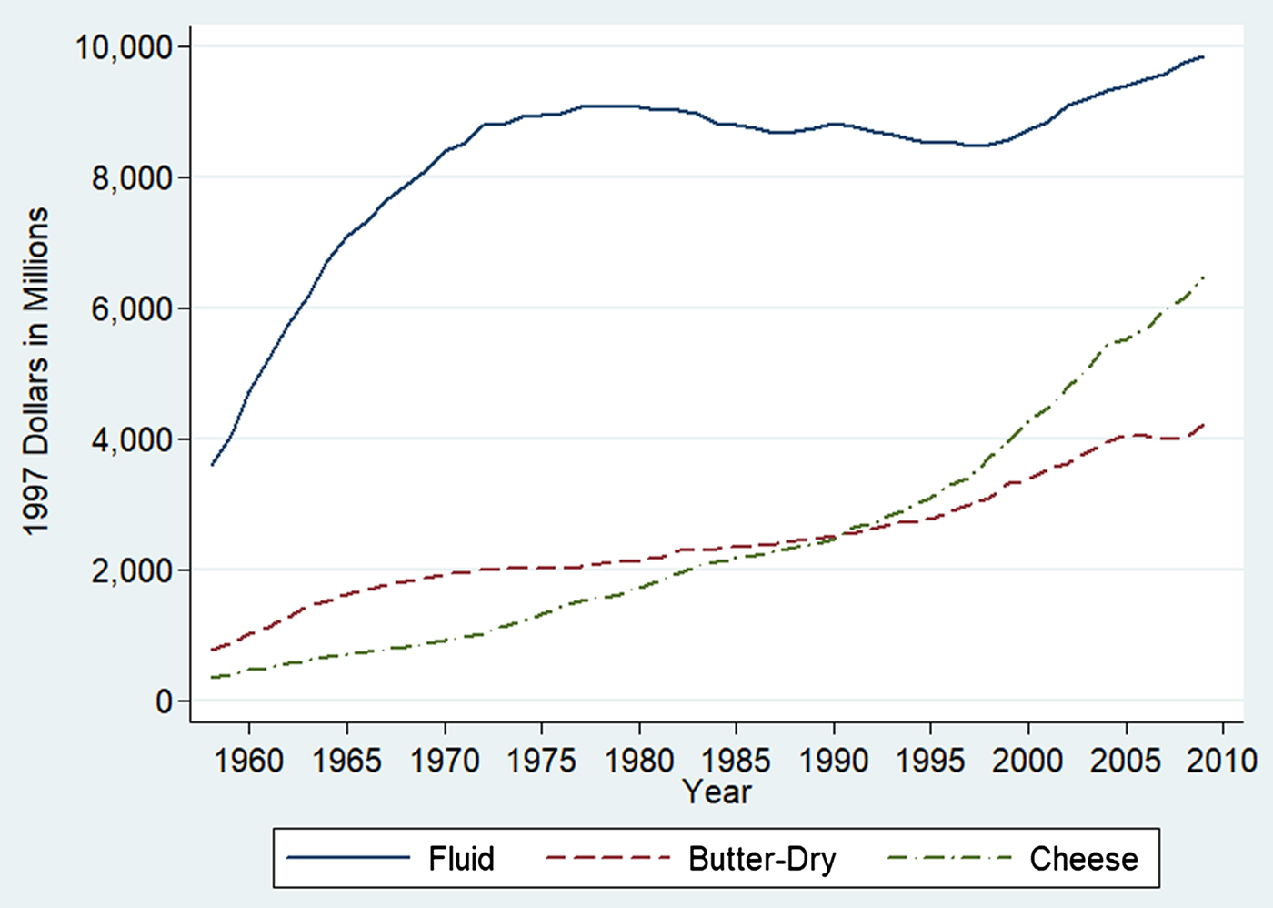
We considered more than one method for measuring capital expenditure and the rental price of capital. First, we constructed a measure of capital expenditure using data in the NBER database on capital stocks. The NBER database includes data on real capital stocks of equipment and structures, which are constructed using the data on net capital stocks from the Federal Reserve Board (FRB) (Bartelsman and Gray Reference Bartelsman and Gray1996, Becker, Gray, and Marvakov Reference Becker, Gray and Marvakov2013). The FRB data on net capital stock are constructed using a perpetual inventory model (Mohr and Gilber Reference Mohr and Gilber1996). Figure 1 plots real capital stocks for the three dairy industries. The capital stock of the fluid dairy industry is much larger than those of the other two industries.
Real Capital Stocks of the Dairy Industries
Estimates of nominal rental prices were obtained from the Bureau of Labor Statistics (BLS). The BLS estimates of rental prices take account of the nominal rates of return to capital assets, the nominal rates of economic depreciation, and revaluation of assets. Rental prices are also adjusted for the effects of taxes (USBLS 2006, 2007). In constructing the rental prices, BLS computes an “internal rate of return,” i t in equation 4, using data on property income taken from the National Income and Product Accounts (Jorgenson and Griliches Reference Jorgenson and Griliches1967). The BLS assumes a hyperbolic depreciation pattern to compute δt, such that assets lose efficiency at a slow rate early in their life and at a much faster rate as they age (Dean and Harper Reference Dean and Harper1998). We use the estimates of the rental prices of structures and equipment for the food and beverage and tobacco industry. Then, the rental price of capital is constructed as a weighted average of rental prices of structures and equipment, using stocks of industry-specific structure and equipment as weights.
In addition to using the rental prices from the BLS, we also considered constructing rental rates under simplifying assumptions: (1) the rate of economic appreciation of new asset prices is the same as the rate of general inflation, (2) a constant geometric rate of depreciation, and (3) a constant real interest rate. Under these assumptions, equation 4 becomes ρt = P t (r + δ), where r is the real interest rate (equal to the nominal interest rate i minus the rate of general inflation). Here r is assumed to be 0.03. Using an average service life of 25 years, and assuming that an asset is retired when its productive efficiency falls below 15 percent, we calculated that δ = 0.07.Footnote 6 The NBER database includes nominal price indices for new investments in equipment and structures (P t). We computed rental prices, ρt, according to ρt = P t (r + δ) = P t × 0.1.
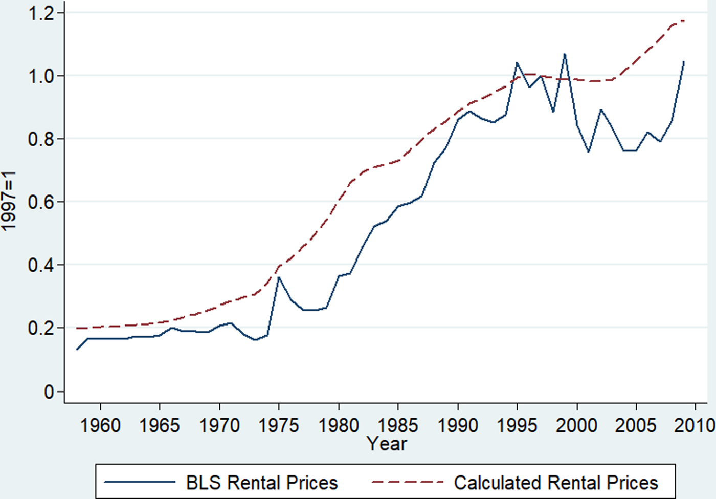
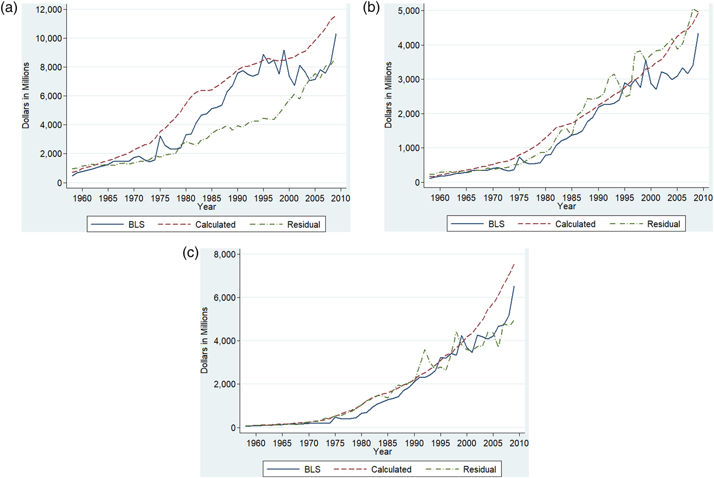
Figure 2 plots nominal rental prices obtained from the BLS and those constructed under the above simplifying assumptions. The two series trace each other relatively well, but the BLS rental prices are more volatile. Using the data on real capital stocks from the NBER database and rental rates of capital either obtained from BLS or calculated by ourselves, we constructed measures of capital service flows and rental expenditure. We also calculated the rental expenditure of capital as the residual that exhausts the value of output. Figure 3 plots the three different measures of rental expenditure for each dairy processing and manufacturing subindustry. For the butter-dry industry and the cheese industry, the differences between the different measures of rental expenditure are relatively small. For the fluid industry, the two measures of capital expenditure constructed using the NBER measure of capital stock deviate significantly from the residual measure of capital expenditure. This is clearly driven by the measure of capital stock of the fluid industry.
Indices of Nominal Rental Prices
Nominal Rental Value of Capital of the Dairy Industries (a) Fluid (b) Butter-Dry (c) Cheese
In the estimation, we assume constant returns to scale at the industry level and use the residual that exhausts the value of output as the rental expenditure on capital. We estimated the models using both measures of rental prices, and the results are not qualitatively different. The reported results were obtained using the BLS rental prices. Table 1 summarizes the cost shares of inputs for each industry over the sample period. The cost shares of capital have been increasing, especially during the 1990s, and the shares of labor have been decreasing, especially for the fluid industry.
Average Cost Shares of Inputs of the U.S. Dairy Industry, 1958–2009

Notes: Average shares are weighted averages of the three industries using as weights each industry's share of the value of output.
Empirical Implementation and Results
This section first discusses the two flexible functional forms for the cost function that we use in the econometric estimation. We then present results from the seemingly unrelated regressions (SUR). Results are also reported for models that use instrumental variable estimation. Results from different models and specifications are qualitatively equivalent and quantitatively similar.
Functional Forms
We consider two locally flexible functional forms in the empirical analysis: the generalized Leontief (GL) (Diewert Reference Diewert1971) and the translog (Christensen, Jorgenson, and Lau Reference Christensen, Jorgenson and Lau1973). Locally flexible functional forms provide a second-order local approximation to an arbitrary twice continuously differentiable function (see chapter 5 of Chambers (Reference Chambers1988) for an introduction to flexible functional forms). A GL cost function is a generalized version of a cost function based on a fixed proportions production function. The specific GL functional form used in this analysis was used by Morrison Paul (Reference Morrison Paul2001) and Morrison Paul and MacDonald (Reference Morrison Paul and MacDonald2003).Footnote 7 A translog form is an extension of the Cobb-Douglas functional form; it is a second- instead of first-order log-linear function. Neither of the functional forms imposes curvature conditions directly, but we can check for violations of the curvature conditions at each data point (Gallant and Golub Reference Gallant and Golub1984). Caves and Christensen (Reference Caves and Christensen1980) have shown that a GL functional form has satisfactory local properties when substitution among inputs is low.
Under the assumption of constant returns to scale, the average cost function for the GL functional form is specified as equation 6.
 $$\eqalign{C\lpar {\bi w}\comma \; t\rpar = & \mathop \sum \limits_i I_i \mathop \sum \limits_j {\rm \beta} _{ij} w_j + \mathop \sum \limits_j \mathop \sum \limits_k {\rm \beta} _{\,jk} w_j^{1/2} w_k^{1/2} + t\mathop \sum \limits_i I_i \mathop \sum \limits_j {\rm \beta} _{ijt} w_j \cr & + {\rm \beta} _{tt} t^2 \mathop \sum \limits_j w_j.} $$
Subscripts j and k denote inputs, and I i with i ∈ {1, 2, 3} denote the fluid, butter-dry, and cheese subindustries, respectively. We estimate the model using pooled data and industry dummy variables are included in a manner that linear homogeneity in input prices is maintained. We also allow the coefficient of the time-trend to vary by industry to capture different rates of technical change among the three industries. The other parameters, βjk, representing input demand relationships, are held constant across the three industries. Applying Shephard's lemma to equation 6 yields input-output demand equations, which are the demand functions for inputs per unit of output for the GL model. For example, the input-output demand equation for energy is
 $$\displaystyle{{x_E} \over y} = \mathop \sum \limits_i {\rm \beta} _{iE} I_i + \mathop \sum \limits_{k \ne E} {\rm \beta} _{Ek} w_k^{1/2} w_E^{ - 1/2} + t\mathop \sum \limits_i {\rm \beta} _{iEt} I_i + {\rm \beta} _{tt} t^2. $$
The average cost function for the translog functional form is specified as:
 $$\eqalign{lnC({\bi w},t) = & \mathop \sum \limits_i {\rm \alpha} _i I_i + \mathop \sum \limits_i I_i \mathop \sum \limits_j {\rm \alpha} _{ij} lnw_j + \displaystyle{1 \over 2}\mathop \sum \limits_j \mathop \sum \limits_k {\rm \alpha} _{\,jk} lnw_j lnw_k \cr & + t\mathop \sum \limits_i {\rm \alpha} _{it} I_i + t\mathop \sum \limits_i I_i \mathop \sum \limits_j {\rm \alpha} _{ijt} lnw_j.} $$
Applying Shephard's lemma to equation 8 yields input cost share equations for the translog model. For example, the energy share equation is
 $$s_E = \mathop \sum \limits_i {\rm \alpha} _{iE} I_i \; + \mathop \sum \limits_k {\rm \alpha} _{Ek} lnw_k + t\mathop \sum \limits_i {\rm \alpha} _{iEt} I_i. $$
When using a GL functional form, the estimating system consists of the average cost function and input-output demand equations for capital, labor, energy, milk, and other processing materials. Linear homogeneity of the cost function in input prices is satisfied with this specific GL functional form. When using a translog functional form, we estimate a system of equations consisting of the average cost function and cost share equations. Linear homogeneity of the cost function is accomplished by normalizing the average cost and the prices of capital, labor, energy, and milk by the price of other materials.
SUR Estimation
We first estimate the econometric models using the SUR. In addition to linear homogeneity, symmetry of the Hessian matrix is imposed. Most of the parameter estimates are statistically significant. See Appendix A for details. Table 2 presents the price elasticities of input demand at the mean of sample data for each subindustry. Standard errors are in parentheses. Elasticity estimates are nonlinear functions of model parameters, so the standard errors are obtained by applying the bootstrap method with replacement for 1,000 iterations (Eakin, McMillen, and Buono Reference Eakin, McMillen and Buono1990, Krinsky and Robb Reference Krinsky and Robb1991). Most of the elasticity estimates are statistically significant, except for some of the estimates related to energy. Estimates from the two functional forms differ the most for the cheese industry. The estimates of elasticities differ across the two functional forms, especially for energy, but the same economic implications can be drawn from both models.
Output-Constant Price Elasticities of Input Demand in the U.S. Dairy Industry, 1958–2009
Notes: Numbers in this table refer to the price elasticity of demand, evaluated at the sample means, for the input in a row with respect to changes in the price of the input in a column while holding output constant. Numbers in parentheses refer to standard errors, obtained by applying the bootstrap method with replacement for 1,000 iterations.
In summary, the input demands are all inelastic. The estimates indicate that the industry-specific own-price elasticities of demand for inputs are between −0.48 and −0.84 for capital, between −0.31 and −0.72 for labor, between −0.06 and −0.74 for energy, between −0.09 and −0.18 for milk, and between −0.26 and −0.60 for other processing materials. The demand for milk is the least elastic, as expected. We devote the next section to further discussions of the derived demand for farm milk. These estimated elasticities are consistent with the findings of Goodwin and Brester (Reference Goodwin and Brester1995) and Morrison Paul and MacDonald (Reference Morrison Paul and MacDonald2003) for the U.S. food manufacturing industry.
The estimates of the cross-price elasticities vary across industries but imply similar substitute or complementary relationships. Capital, energy, and other processing materials are estimated to be substitutes for milk, while labor is estimated to be a complement for milk, but the estimated elasticities are fairly small. Capital and energy are likely to be used in fixed proportions: the cross-price elasticities are all small and statistically insignificant. As expected, the category “other processing materials” is estimated to be a substitute for all other inputs.
Table 3 summarizes the elasticities of the average cost and input demands with respect to the time-trend variable. The average cost of production for the fluid industry would have decreased by 0.3 percent per year, holding input prices constant; while ηCt is estimated to be positive for the butter-dry and cheese industries. Estimates from both functional forms imply that technical change has been capital using and labor saving for all three subindustries, which is plausible given the movements of the relative price of capital to labor. To put the estimates into perspective, we calculate the term ηjt − ηCt in the definition of technical change bias, which measures the proportional change in the cost shares of inputs holding input prices constant. By this measure, based on the translog estimates, the cost share of capital would have increased by 0.5 percent, 1.9 percent, and 0.8 percent per year for the fluid, butter-dry, and cheese industries, respectively, and the cost share of labor would have decreased by 2.2 percent, 1.2 percent, and 1.8 percent per year for the fluid, butter-dry, and cheese industries, respectively. For the other inputs, point estimates from the translog specification indicate that technical change has been energy using for all three dairy industries, with a statistically significant estimate for cheese manufacturing, and materials using for butter-dry and cheese manufacturing.
Rates and Biases of Technical Change in the U.S. Dairy Industry, 1958–2009
Notes: Numbers in this table refer to the proportional change of the variable in a row for a unit change in the time-trend variable, multiplied by 100, thus measuring the annual percentage changes in the variable attributed to technical change.
The dairy manufacturing industry has been through numerous changes in the past fifty years. The number of dairy processing facilities has decreased significantly, while the average size of facilities increased. The number of dairy products has also increased. One caveat of our analysis is that we do not model plant-level economies of scale and scope for dairy processors and manufacturers. Given that the purpose of our analysis is to provide relevant parameters for evaluating the impacts of direct and indirect policies on the U.S. dairy manufacturing industry as a whole, we are content to relegate analysis of firm and industry dynamics to other studies.
Instrumental Variable Estimation
As mentioned above, we are not particularly concerned with the endogeneity of explanatory variables in this analysis, because the dairy manufacturing industry is not a significant player in the markets for most of its inputs, and the price of milk is influenced by federal and state milk marketing orders. For a robustness check, we provide estimates of the elasticities from instrumental-variable estimation using three-state least squares (3SLS). We use a set of supply-side variables and macroeconomic variables as instruments for the price of milk: the price of corn, cow inventory per capita, population, gross domestic product per capita, corporate income tax rate, personal labor income tax rate, and the price of oil. We estimated the model with different sets of instruments, but the elasticity estimates are closely similar across different combinations of instruments. Moreover, we fail to reject the null hypothesis of the Hausman specification test, indicating that there is no systematic difference between the instrumental variable estimation and the SUR estimation. Table 4 summarizes the 3SLS estimates of the price elasticities of input demand at the mean of the data for each of the three dairy processing and manufacturing subindustries, and Table 5 presents the 3SLS estimates of the elasticities of the average cost and input demands with respect to the time-trend variable. Comparing the estimates from Tables 4 and 2 and from Tables 5 and 3, none of the 3SLS estimates is qualitatively different from the SUR estimates.
Price Elasticities of Input Demand in the U.S. Dairy Industry, 1958–2009: 3SLS

Notes: See notes to Table 2.
Rates and Biases of Technical Change in the U.S. Dairy Industry, 1958–2009: 3SLS
Notes: See notes to Table 3.
Derived Demand for Farm Milk
The demand for farm milk is not a consumer demand, but rather a derived demand for an input used by the dairy manufacturing industry. Therefore, estimates of the price elasticities of demand for dairy products are not directly comparable to estimates of the price elasticity of demand for farm milk. Moreover, a fixed relationship does not exist between the price elasticities of demand for final products and the elasticities of derived demand for inputs (Wohlgenant Reference Wohlgenant1989, Reference Wohlgenant, Gardner and Rausser2001). However, when the industry can be modeled as exhibiting constant returns to scale, with perfectly competitive output markets, the relationship defined in equation 10 between the price elasticity of derived demand for milk and price elasticities of demand for the final products holds:
 $${\rm \eta} _{MM}^1 = {\tilde\eta}_{MM}^1 + {\rm \eta} ^{11} s_M^1 + {\rm \eta} ^{12} s_M^2 + {\rm \eta} ^{13} s_M^3 $$
where  ${\rm \eta} _{MM}^1 \; $ denotes the Marshallian own-price elasticity of demand for milk used in product 1, ${\tilde\eta} _{MM}^1 $ is the output-constant (Hicksian) own-price elasticity of demand for milk used in product 1, η11 is the own-price elasticity of demand for product 1, η12 and η13 are the elasticities of demand for product 1 with respect to the prices of products 2 and 3, respectively, and $s_M^1 $, $s_M^2 $, and $s_M^3 $ are the shares of milk in the cost of producing products 1, 2, and 3. Similar relationships hold for ${\rm \eta} _{MM}^2 $ and ${\rm \eta} _{MM}^3 $.
In using a cost function framework to estimate the input demand relationships of the dairy manufacturing industry, we have estimated the output-constant own-price elasticities of demand for farm milk ( ${\tilde\eta} _{MM}^i $) for the three dairy industries analyzed in this paper—fluid, butter-dry, and cheese. Using equation 10, we can obtain “synthetic” estimates of Marshallian own-price elasticity of demand for farm milk. To calculate the Marshallian elasticity of derived demand for milk, we use the estimates of output-constant elasticities reported in Table 2 and estimates of price elasticities of demand for dairy products from the literature.
Published estimates of the own-price elasticity of retail demand in the United States range from −0.04 to −1.70 for fluid milk (Heien and Wessells Reference Heien and Wessells1988, Huang Reference Huang1993, Schmit and Kaiser Reference Schmit and Kaiser2004, Alviola and Capps Reference Alviola and Capps2010, Chouinard et al. Reference Chouinard, Davis, LaFrance and Perloff2010, Davis et al. Reference Davis, Dong, Blayney and Owens2010), and range from −0.08 to −1.87 for other dairy products. Export demand for manufactured dairy products has become substantial, so it is necessary to construct the elasticity of demand for butter-dry or cheese as a weighted average of the domestic demand elasticity and the export demand elasticity. Export demand elasticities for manufactured dairy products produced in the United States are not readily available from the literature. A full-blown analysis of export demand for U.S. dairy products is beyond the scope of this paper. We use −0.5, −3.0, and −3.0 as our best estimates of the own-price elasticities of demand for fluid, butter-dry, and cheese dairy products, respectively, reflecting both U.S. domestic and export demand responses. To illustrate the sensitivity of the calculations to the size of these underlying elasticities, we also try a set of less-elastic estimates, equal to 0.5 times the best estimates (i.e., −0.25, −1.5, and −1.5, respectively) and a set of more-elastic estimates, equal to 1.5 times the best estimates (i.e., −0.75, −4.5, and −4.5, respectively). These estimates are consistent with plausible assumptions about underlying national elasticities of demand, elasticities of price transmission, and trade flows.Footnote 8 Cross-price elasticities of demand for different dairy products are small. Following Balagtas and Kim (Reference Balagtas and Kim2007), we use 0.02 as an estimate of all the cross-price elasticities of demand for dairy products.
We use the average cost shares of milk in the production for the years 2005–2009 to calculate the elasticities of derived demand for farm milk. Table 6 presents the results. We calculate the elasticities of derived demand for farm milk using both the GL and the translog estimates of the output-constant own-price elasticities of demand for milk. The calculated Marshallian own-price elasticity of demand for milk is between −0.16 and −0.39 for fluid dairy products, between −0.68 and −1.95 for butter-dry dairy products, and between −0.60 and −1.69 for cheese; the “best” estimates of these elasticities are about −0.2, −1.3, and −1.1, respectively.
Elasticities of Derived Demand for Milk

Notes: The GL and translog estimates of output-constant own-price elasticities of demand for milk from Table 2 are used in these calculations. i = 1, 2, 3 for the fluid, butter-dry, and cheese industries, respectively.
The aggregate elasticity of derived demand for farm milk can be calculated as follows,
 $${\rm \eta} _{MM} = {\rm \theta} _M^1 {\rm \eta} _{MM}^1 + {\rm \theta} _M^2 {\rm \eta} _{MM}^2 + {\rm \theta} _M^3 {\rm \eta} _{MM}^3\comma \; $$
where  ${\rm \theta} _M^1 $, ${\rm \theta} _M^2 $, and ${\rm \theta} _M^3 $ represent the shares of milk used for industries 1, 2, and 3. The aggregate elasticity of derived demand for milk is calculated using the average shares of milk used for the final products for the years 2005–2009, which are also reported in Table 6. In aggregate, our estimates indicate that the own-price elasticity of demand for farm milk is in the range of −0.43 to −1.20, and our best estimate, calculated using our preferred parameter values, is about −0.80. Given that we use estimates of the elasticities of demand for dairy products from the literature to calculate the elasticities of derived demand for milk, the reliability of these synthetic estimates depends partially on the quality of the studies from which some estimates were drawn. Future research may involve a thorough meta-analysis of the studies on the demand for U.S. dairy products, including export demand, so that we can calculate measures of precision for these synthetic estimates of the own-price elasticity of demand for farm milk, or new estimates of elasticities of demand for dairy products.
Conclusion
The dairy industry is an important part of the U.S. agricultural and food system. Dairy manufacturing adds significant value to farm milk. Understanding the input demand relationships in this industry is essential for quantifying the effects of changes in the markets for dairy products, milk, and other inputs, and changes in regulations and technology. For example, dairy support policies, ranging from the Dairy Price Support Program to margin-based programs, such as the Margin Protection Program for Dairy Producers, can be linked to the price of farm milk (Balagtas and Sumner Reference Balagtas and Sumner2012). The price elasticity of demand for farm milk is an essential parameter in evaluating the consequences of these programs. As another example, to quantify the effects of carbon-pricing policies on dairy manufacturing, it is crucial to assess the potential for substitution between energy and other inputs under current technology, and the long-run potential for energy-saving technical changes.
In this study, we utilize the distinctive features of production, policy, and industrial organization in the U.S. dairy manufacturing industry to evaluate input demand and the nature of technical change in this industry. Using annual data from 1958 to 2009 on three subindustries—the processing of fluid and soft dairy products, the manufacturing of butter and dry dairy products, and cheese manufacturing—we estimate the parameters of the cost system for the dairy manufacturing industry. Two flexible functional forms and different estimation methods are employed to provide robustness checks. A significant contribution of the work is to develop and explore the implications of alternative approaches to measure the ever-challenging capital stock and its rental price.
Using estimated parameters of the cost function, we first obtain a set of output-constant price elasticities of demand for farm milk. We then calculate the Marshallian price elasticities of demand for farm milk by combining our estimated output-constant elasticities with estimates of the price elasticities of market demand for dairy products from the literature. In aggregate, we estimate that the Marshallian own-price elasticity of demand for farm milk is about −0.80. Estimates of the cross-price elasticities indicate that capital, energy, and other processing materials are substitutes for milk, while labor is a complement for milk. Among other inputs, capital and energy are likely to be used in fixed proportions and other processing materials is a substitute for all other inputs. Our estimates also indicate that technical change has lowered the average cost of production for the fluid industry, and that technical change has been capital using and labor saving for all three dairy industries. For other inputs, results of some specifications show that technical change might have been energy and materials using.
Appendix A. Estimates of Model Parameters
This appendix summarizes estimates of the parameters in equations 6 and 8 using SUR.
Parameter Estimates of Equation 6

Parameter Estimates of Equation 8
Appendix B. Modeling Changes in the Service Flow of Capital
In this appendix, we explore how changes in the “effective” service flow of capital affect input demand and technical change in the U.S. dairy manufacturing industry. In particular, we incorporate capital quantity into a cost function and include an implicit optimization equation for capital in the estimation system. Two indicators are used to model shifts in the “effective” service flow of capital. A post-1970 indicator is used to reflect changes in capital composition to produce a new mix of products in the 1970s and 1980s and a post-1990 indicator is used to capture changes in capital composition to utilize new packaging and to comply with new food-safety and environmental regulations.
We use for this exercise the GL functional form, which tends to generate fewer curvature violations than the translog form, for a model of a restricted cost function (Morrison Paul Reference Morrison Paul1999). The average cost function is specified as equation B1 and the input-output demand for energy, for example, is specified as equation B2. I d is a vector of dummy variables denoting the three time periods: 1958–1969, 1970–1989, and 1990–2009. This GL functional form accommodates both different rates and factor biases of technical change among the three industries and varying effective service flow of capital across the three time periods.
 $$\eqalign{C = & \mathop \sum \limits_{\rm i} I_i \mathop \sum \limits_j {\rm \beta} _{ij} w_j + \mathop \sum \limits_j \mathop \sum \limits_k {\rm \beta} _{\,jk} w_j^{1/2} w_k^{1/2} + t\mathop \sum \limits_i I_i \mathop \sum \limits_j {\rm \beta} _{ijt} w_j \cr &+ x_K \mathop \sum \limits_d I_d \mathop \sum \limits_d {\rm \beta} _{djK} w_j + \lpar {\rm \beta} _{tt} t^2 + {\rm \beta} _{KK} x_K^2 + tx_K \mathop \sum \limits_i {\rm \beta} _{itK} I_i \rpar \mathop \sum \limits_j w_j\comma }$$
 $$\eqalign{\displaystyle{{x_E} \over y} = & \mathop \sum \limits_i {\rm \beta} _{iE} I_i + \mathop \sum \limits_{k \ne E} {\rm \beta} _{Ek} w_k^{1/2} w_E^{ - 1/2} + t\mathop \sum \limits_i {\rm \beta} _{iEt} I_i + x_K \mathop \sum \limits_d {\rm \beta} _{dEK} I_d \cr & + {\rm \beta} _{tt} t^2 + {\rm \beta} _{KK} x_K^2 + tx_K \mathop \sum \limits_i {\rm \beta} _{itK} I_i.}$$
At equilibrium, the optimal quantity of capital services is determined by the condition that the rental rate of capital is equal to the magnitude of the reduction in variable cost resulting from an additional unit of capital input. Using w K to denote the rental rate of capital, this condition implies that w K = −(∂C/∂x K) in equilibrium. When using this GL functional form, the equilibrium condition implies the following estimating equation:
 $$- w_K = \mathop \sum \limits_d I_d \mathop \sum \limits_j {\rm \beta} _{djK} w_j + \lpar 2{\rm \beta} _{KK} x_K + t\mathop \sum \limits_i {\rm \beta} _{itK} I_i \rpar \mathop \sum \limits_j w_j.$$
Tables B1–B3 summarize, respectively, the estimates of the price elasticities of demand for inputs during each time period for each of the three industries. These estimates are calculated at the means of data during each time period for each industry. The standard errors are obtained by applying the bootstrap method with replacement for 1,000 iterations. The signs of the elasticities indicating whether inputs are substitutes or complements remain the same as those estimated without modeling changes in capital composition. However, the precision of the estimates is lower than the estimates in Table 2, especially for energy. Estimates indicate that the own-price elasticity of demand for capital increased in both the 1970s and 1980s and the 1990s and 2000s for the fluid manufacturing industry. On the other hand, the demand for capital in the butter-dry industry is estimated to have become less elastic after 1970. Similar to the butter-dry industry, our estimates show that the demand for capital in the cheese manufacturing industry became substantially less elastic in the 1970s and 1980s, but slightly more elastic after 1990. For all three dairy industries, the estimated demand for other processing materials became more elastic after 1990. For the rest of the inputs, because of the large standard errors, in most cases we would fail to reject the null hypothesis that the own-price elasticities are equal across time periods at a conventional level of significance.
Output-Constant Price Elasticities of Input Demand in the Fluid Industry, 1958–2009
Output-Constant Price Elasticities of Input Demand in the Butter-Dry Industry, 1958–2009

Output-Constant Price Elasticities of Input Demand in the Cheese Industry, 1958–2009

Table B4 summarizes the estimates of the elasticities of the average cost and input demands with respect to the time-trend variable. These estimates indicate that technical change has been capital using, materials using, and labor saving for all three industries throughout the study period, though some of the estimates are imprecise. Holding input prices constant, estimates from this model do not provide evidence of decreases in the average costs of production over time.
Rates and Biases of Technical Change in the U.S. Dairy Industry, 1958–2009


 Open access