ISMIP-HEINO Set-Up

The set-up of the ISMIP-HEINO experiment is given in http://www.pik-potsdam.de/calov/heino/he_setup_2006_11_02.pdf. The model domain is depicted in Figure 1. The region of ‘Hudson Bay’ and ‘Hudson Strait’ (ABCD ∪ EFGH) represents the sedimentary basin, and the rest of the base is assumed to be coarser bedrock. The accumulation rate, b, prescribed as a linear function of the distance, d, from the domain center, increases from a minimal value, b _min at d = 0, to a maximal value, b _max at d = D:

(1)

Immediate calving is prescribed for distances d > D. The surface temperature is defined as

(2)

where S _T is the surface temperature gradient, and a homogeneous geothermal heat flux is prescribed at the glacier base. The ice rheology is governed by Glen’s flow law (Reference GlenGlen, 1955). The values of the physical parameters involved are given in Table 1. The sliding law differs according to the region. For the sedimentary basin (in Hudson Bay and Hudson Strait) the basal sliding velocity, v_b, obeys a linear relation

(3)

while for the coarser part the sliding is assumed to be Weertman-type:

(4)

where is the absolute temperature at the glacier base relative to the pressure melting,

(5)

with β the Clausius–Clapeyron constant, p the pressure, the normal stress at the base, the tangential basal stress, t_αβ the components of the Cauchy stress tensor at the base, and C _S, C _R the sliding parameters. If temperature is below the pressure-melting point, the frozen-bed condition is applied:

(6)

Fig. 1.

Model domain of the ISMIP-HEINO experiment. The ocean is shaded in dark gray; the sedimentary basin is the light gray square ABCD and rectangle EFGH, representing the ‘Hudson Bay’ and ‘Hudson Strait’, respectively. The remaining land (in white) corresponds to coarser bedrock.

Table 1.

Values of the physical parameters for ISMIP-HEINO reference simulation ST (from Reference CalovCalov and others, 2010)

For all simulations, the horizontal resolution of the numerical model is 50 km, which corresponds to 81 × 81 gridpoints in the horizontal plane. The vertical resolution is specified by 61 equally spaced gridpoints in the ‘stretched’ vertical coordinates (when the glacier geometry is mapped to a layer of uniform thickness). The time-step is 0.25 years. The ice sheet is built up from initial ice-free conditions over a time interval 0–200 ka. A total of eight model simulations are examined: ST, T1, T2, S1, S2, S3, B1 and B2, which may be divided into the following four groups, according to the quantity varied in the experiment:

Overview of ISMIP-HEINO Results

The results of the ISMIP-HEINO experiment are outlined in detail by Reference CalovCalov and others (2010). In total, nine models participated in the benchmark, eight of which were based on the shallow-ice approximation (SIA) (Reference HutterHutter, 1983; Reference MorlandMorland, 1984) while one represented a combination of the SIA and shallow-shelf approximation (SSA) approach (Reference Morland, Van der Veen and OerlemansMorland, 1987; Reference MacAyealMacAyeal, 1989). Each participating model exhibits oscillations for at least one model set-up of the total number of eight introduced simulations. These findings therefore support the idea that the HEs are caused by a mechanism involving an intrinsic thermomechanical instability. All models display an enhanced tendency to oscillate when the surface temperature and accumulation rate are decreased. However, a more detailed inspection of the results reveals significant differences in the behavior of the models. While two models (‘b’ and ‘d’) oscillate for all eight simulations, model ‘h’ does so for only one experiment; the response of the other models lies between these two limits. The HEINO experiments also display a satisfactory agreement with respect to reproducing the HE-like oscillations at periods from 5 to 15 ka, which is in relatively good agreement with the geological evidence (Reference HeinrichHeinrich, 1988). However, the monitored output quantities, i.e. the melt fraction and ice thickness averaged over the sedimentary basin, when they are plotted as functions of time, differ significantly from model to model in terms of their shape and the precise timing of the oscillations (if they occur), and, in addition, in the mean value. The Fourier amplitude spectra used to characterize the frequency content of signals show a rather poor agreement in shape, number and position of significant frequency peaks. These differences are puzzling in view of the overall similarity of the applied numerical approaches. As the models (except for model ‘h’) are all of the SIA type, much better consistency and agreement between the results should be expected.

To better quantify the differences in the results, we first introduce a novel spectral tool based on wavelet analysis. The reason for wavelet analysis rather than Fourier analysis is that for the ice-thickness time series, if they oscillate (mainly in experiments ST, T1, B1, S3), the oscillations are not precisely periodic since the lag between two subsequent oscillations appears to be a random quantity. For such a signal, the Fourier spectrum becomes distorted even for a relatively elementary quasi-periodic signal, as a consequence of the global support of the Fourier basis functions (see Appendix). To obtain a better insight into the principal periods present in a quasi-periodic signal, time-localized basis functions are needed. We develop a focused global wavelet spectrum (FGWS), which is derived from the traditional continuous wavelet spectrum (CWS) (see Appendix for details). The FGWS makes use of the information redundancy of the CWS, allowing its modification without affecting the reconstructed time-domain signal. Our modification is designed to give a better spectral resolution than the CWS for a certain class of quasi-periodic signals, having the same basic characteristics as the investigated ISMIP-HEINO ice-thickness output signal.

We choose a particular mother wavelet function (see Appendix) such that there is a correspondence between the scales of the wavelet spectra and the periods in the Fourier amplitude spectrum. The FGWS can then be compared with the Fourier amplitude spectrum. Figure 2 compares the FGWS and the normalized Fourier amplitude spectrum, truncated at the period T = 25 ka, for the original ISMIP-HEINO average ice-thickness time series over the sedimentary basin for experiment ST. The time-series data have been kindly provided by R. Calov and other ISMIP-HEINO participants (http://www.pik-potsdam.de/calov/heinodata.html).

Fig. 2.

The normalized amplitude Fourier spectrum (left) and the FGWS (right), truncated at a period of 25 ka for the participating models a–i in the ST ISMIP-HEINO experiment.

We can see that the FGWS are more localized than the Fourier amplitude spectra and provide a better insight into the principal periods contained in the signals. The FGWS also shows large differences between the models. Despite distinct numbers of spectral peaks present in the FGWS, the amplitudes of these peaks differ significantly, and their positions vary between 5 and 20 ka.

Description and Validation of the Novel 3-D Thermomechanical Ice-Sheet Model

This study uses a novel numerical ice-sheet model, JOSH (JOint Shallow-ice/Higher-order model), which combines the traditional SIA with a higher-order approach based on the SIA-I algorithm developed by Reference Souček and MartinecSouček and Martinec (2008). This algorithm computes the SIA in the first step and then iteratively improves the solution. The iterations are based on a procedure analogous to the SIA, but applied only to deviations of the approximate solution from the exact full-Stokes solution. Its ability to capture higher-order effects by including the longitudinal stresses has been demonstrated in the ISMIP-HOM experiment (Reference PattynPattyn and others, 2008; model oso1). We implemented the SIA-I algorithm into an evolutionary three-dimensional (3-D) thermomechanical ice-sheet model. A finite-difference technique is applied for discretizing the governing equations, i.e. the SIA-I linear momentum and rheology equations, the kinematic equation for a free glacier surface and the heat-transport equation. The SIA-I algorithm uses a simple Arakawa A grid (Reference Arakawa, Lamb and ChangArakawa, 1977) for discretization, i.e. each node contains all the field variables. Details of the numerics are given by Reference SoučekSouček (2010).

To verify the capability of JOSH to perform thermomechanically coupled ice-sheet simulations, we benchmark it following the EISMINT experiments (A, B, C, D, G) from the exercise ‘Effect of thermomechanical coupling’ (Reference PaynePayne and others, 2000). These experiments compare the steady-state geometry and the thermodynamic state of an axisymmetric ice sheet whose evolution is simulated from initially ice-free conditions under a prescribed steady climatic forcing. In addition, the effect of variations in climate forcing on the resultant steady state is investigated. Table 2 shows our results for both the SIA and the HO modes, together with the published EISMINT results. For the HO simulations, we used 20 SIA-I iterations with projection parameters Θ₁ = 0.2 and Θ₂ = 0.2 (Reference Souček and MartinecSouček and Martinec, 2008). Table 2 shows that JOSH is capable of reproducing the EISMINT results with sufficient accuracy. It also provides us with a crude estimate of the effect of HO dynamics for such a type of experiment. The differences between our SI and HO simulations by JOSH confirm the findings of a different HO model by Reference PattynPattyn (2003). Employing the HO approximation results in a slightly thinner ice sheet (∼40 m difference at the ice divide for experiment A) and a slightly warmer base (∼2 K at the base below the ice divide for experiment A). Note that the differences between the HO and the SI results are approximately of the same order as the range among the published SIA-based EISMINT models.

Table 2.

EISMINT experiment A, B, C, D, G results. V: glaciated volume; A: glaciated area; f: melt fraction at the glacier bed; h: ice-divide thickness; T: basal temperature below the ice divide; Δ _{X − Y} : change of a quantity between experiments X and Y. Two sets of results are displayed forthe JOSH model: the SIA simulations and the HO simulations by the SIA-I algorithm. The EISMINT averages and ranges for the investigated quantities are reprinted for comparison from Reference PaynePayne and others (2000)

ISMIP-HEINO Results for the Josh Model

SI mode

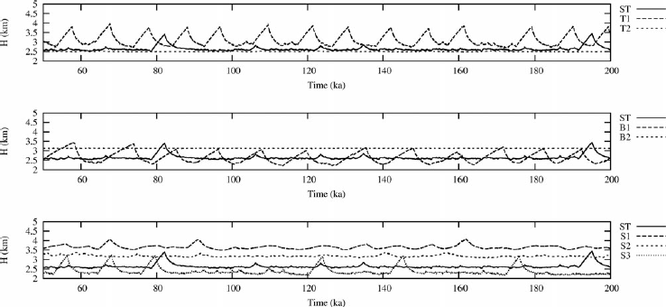
We first recomputed the ISMIP-HEINO experiments in the SI mode by performing only the first iteration of the SIA-I algorithm. In Figure 3, the time series of averaged ice thickness over the sedimentary basin for the three types of experiments (T1, T2), (B1, B2), (S1, S2, S3) are shown and compared with the reference simulation, ST. We plot the results for the time interval 50–200 ka of simulation time, during which the ice sheet is already fully developed. In Figure 4, the Fourier amplitude spectra truncated at the period of T = 25 ka and normalized to unity over this interval are shown, while in Figure 5 we present the corresponding FGWS.

Fig. 3.

The average ice thickness, H, over the sedimentary basin for experiments ST, T1, T2 (top panel), ST, B1, B2 (middle panel) and ST, S1, S2, S3 (bottom panel), for the ISMIP-HEINO experiments with the JOSH model in SI mode.

Fig. 4.

The normalized Fourier amplitude spectra of the time series of Figure 3 truncated at 25 ka.

Fig. 5.

Same as Figure 4, but for the FGWS.

We observe that only few oscillations are generated by JOSH for the reference ST simulation, but significant oscillations occur in the T1 experiment (a colder surface), the B1 experiment (a reduced accumulation rate) and the S3 experiment (fast sliding over the sedimentary basin). This is in good qualitative agreement with results of the ISMIP-HEINO experiment, as all three conditions favor repeated refreezing of the glacier base after a period of rapid sliding. Note that the dominant period in the FGWS for all significantly oscillating signals is ∼10 ka.

HO mode (SIA-I)

The T1 experiment, which exhibits clear oscillations, is taken as a reference simulation for investigating the effect of the HO approximation in the ice-flow equations. The HO approximation is implemented by the SIA-I algorithm (Reference Souček and MartinecSouček and Martinec, 2008) (using 20 SIA-I iterations and projection parameters Θ₁ = 0.2, Θ₂ = 0.2). The SIA-I algorithm converges to a solution adjusting the rheology equations exactly and linear momentum equations with an error of O(ε²) (ε being the height/length aspect ratio of the ice sheet). The algorithm is presented in detail by Reference Souček and MartinecSouček and Martinec (2008), and its convergence and accuracy are discussed by Reference SoučekSouček (2010). The SIA-I algorithm solves only the linear momentum and rheology equations. The heat-transport equation is solved in the SI approximation (e.g. Reference GreveGreve, 1997) with the HO advection velocities delivered by the SIA-I. Two different HO simulations are performed. In the first simulation, denoted ‘HO-1’, the sliding law is kept in the SI form, i.e. τ _b in Equations (3) and (4) is taken as

(7)

where ∇ _h H is the horizontal gradient of the ice thickness, H. In the second simulation, denoted ‘HO-2’, a HO approximation of the basal traction, τ _b, obtained by the SIA-I solution is employed in the sliding law, i.e. we take , where and are the components of the HO Cauchy stress tensor at the glacier base.

Both HO simulations are performed for the T1 experiment set-up. The simulations are initiated from ice-free conditions and run for 200 ka with a time-step of 0.25 years. The simulated time series of average ice thickness and the reference T1 SIA solution above the sedimentary basin are shown in Figure 6. In Figure 7 the Fourier amplitude spectra and FGWS for the three simulations (SIA, HO-1, HO-2) are shown. While already visible in the time series, the spectra confirm that (1) the principal periods of HO-1, HO-2 and the SIA oscillations coincide very well, with a tiny shift of the HO-1 spectrum to larger periods compared with the HO-2 spectrum; and (2) the amplitude and number of oscillations relative to the SIA run is slightly decreased in the HO-1 experiment and increased in the HO-2 experiment, resulting in the observed differences in amplitudes of the FGWS.

Fig. 6.

The average ice thickness, H, over the sedimentary area for the T1 experiment, performed in the SI mode (SIA), higher-order mode with the SIA sliding law (HO-1) and fully HO mode (HO-2).

Fig. 7.

The Fourier amplitude spectra (left) and FGWS (right) for experiment T1, performed in the SI mode (SIA), higher-order mode with the SIA sliding law (HO-1) and fully HO mode (HO-2). All spectra are truncated at a period of 25 ka.

Assessing the Robustness of the ISMIP-HEINO Results

Sensitivity study I: effect of surface temperature noise

To assess the robustness of the results from the previous section, we perturb the surface temperature field, T_surf, by spatially non-correlated normal Gaussian noise with the distribution N(0,1) and amplitude ΔT = 0.01 K. The T1 experiment is performed for a number of the realizations of the noise, ΔT · N(0,1), where again the time series and corresponding Fourier amplitude spectra and FGWS for the average ice thickness over the sedimentary basin are monitored. The model response to relatively low levels of noise in the surface temperature, shown in Figure 8 for several time series, is surprisingly strong. We can see that the curves become quickly out of phase after initialization, typically within the characteristic period of the oscillations, which is ∼10 ka for this experiment. Despite the similarity in amplitude and shape of the oscillations, the time series appears chaotic, due to a randomness in the time lag between subsequent oscillations. As a result, the Fourier amplitude spectra, shown in Figure 9, are distorted and poorly resolved. The FGWS, in contrast, are better localized with less distortion. Nevertheless, the dominant period of the FGWS is resolved with an uncertainty of ±2 ka. Since it is unlikely that the applied temperature perturbations should have a considerable impact on the ice-sheet dynamics, the resulting chaotic behavior is to be interpreted as a deficiency in the numerical model, and the value of ±2 ka is to be understood as the uncertainty of the FGWS for the ISMIPHEINO experiments.

Fig. 8.

The average ice thickness, H, over the sedimentary basin for the surface temperature noise perturbations experiment.

Fig. 9.

The Fourier amplitude spectra (left) and FGWS (right) for the time series in Figure 8, truncated at a period of 25 ka.

In view of these results, the differences between the HO and the SI approximations investigated in the previous paragraph are within the uncertainty of the FGWS amplitude and period, and therefore the effect of HO dynamics on the HE oscillations is negligible. Also, the model sensitivity to surface temperature variations suggests a possible interpretation of the differences among the ISMIPHEINO results. We suggest that these differences are caused by the differences in the modelled temperature fields. The following experiment supports this hypothesis.

Sensitivity study II: effect of uncertainty in the modelled temperature field

In the previous subsection we studied the effect of noise in the surface temperature; we now investigate the JOSH model’s response to surface temperature variations with amplitudes corresponding to the uncertainties in the modelled basal temperature fields. This value is not known precisely, but may be estimated from the results of the EISMINT benchmark experiment, exercise ‘Effect of thermomechanical coupling’ (Reference PaynePayne and others, 2000). We inspect EISMINT experiments G and H, which include the physical phenomena influencing the ISMIP-HEINO experiments, i.e. the dynamics of an ice sheet of continental dimension with a temperature-dependent ice rheology and basal sliding either decoupled (experiment G) or coupled (experiment H) with the basal temperatures. The results (Reference PaynePayne and others, 2000, tables 8 and 9) show (after rejecting an obvious outlier – model ‘U’) that there is good agreement in the modelled topography and ice thickness. However, the divide basal temperatures and the basal melt fractions differ significantly. For experiment G, the ice-divide basal temperature varies between 247.700 and 249.482 K and the melt fraction between 0.250 and 0.391; for experiment H, the divide basal temperature is between 253.737 and 256.714 K and the melt fraction between 0.351 and 0.622. Based on these EISMINT discrepancies, we vary the surface temperature uniformly from ΔT = −3 to +3K and investigate the influence in the ISMIP-HEINO experiment ST in the SI mode. The time series in Figure 10 reveal a considerable effect resulting from the ±3 K temperature variations. As expected, the occurrence of HE-like oscillations is most frequent for the coldest (ΔT = −3 K) scenario. With increasing temperature the shape of the ‘shark-tooth’ oscillations does not change, but the time-averaged lag between neighboring oscillations increases until a threshold value of ΔT = +1.2 K, above which oscillations do not occur.

Fig. 10.

Time series of the average ice thickness over the sedimentary area. ISMIP-HEINO ST set-up is modified by uniform surface temperature variations ranging from −3 K (top) to +3 K (bottom).

In Figure 11 the Fourier amplitude spectra and the FGWS are shown for a series of simulations with gradually increasing ΔT. It is not possible to draw any conclusions from the Fourier amplitude spectra, but the FGWS show a tendency of gradually decreasing amplitudes and peak values shifting to longer periods with increasing temperature. This spectral behavior reflects the elongation of the gaps between subsequent oscillations, as observed in the time series in Figure 10. This simulation suggests that small deviations in basal temperature modelling, as deduced from the results of the EISMINT experiment, may significantly affect the occurrence of Heinrich oscillations in the numerical model.

Fig. 11.

The Fourier amplitude spectra (left) and FGWS (right) for uniform surface temperature variation experiments. Both spectra are truncated at 25 ka.

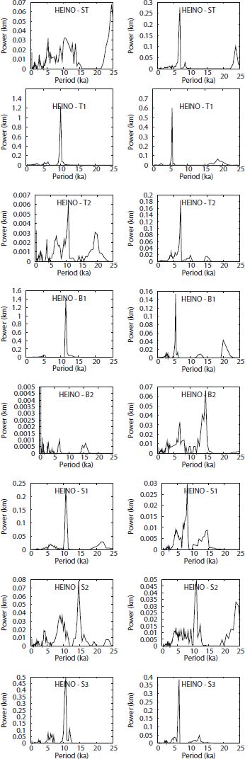
In Figure 12, the FGWS for the published ISMIP-HEINO results (models a–i) are shown. The figure confirms a large variability in the results, both in the FGWS amplitudes and the dominant periods, which typically range from 5 to 15 ka. As shown in Figure 5, our numerical model has a dominant period of ∼10 ka for all significantly oscillating experiments (T1, B1, S3).

Fig. 12.

The FGWS for all ISMIP-HEINO experiments for models a–i.

These results may partially explain the variance among the ISMIP-HEINO dominant periods in the FGWS. If the model temperature rises, the average length of gaps between subsequent oscillations increases, and the FGWS peak is shifted to larger periods. However, by this argument, we cannot explain the converse process: a shift of the dominant peak towards shorter periods, such as 5 ka, clearly visible in Figure 12 for several ISMIP-HEINO models. In addition, by inspecting the time series (http://www.pikpotsdam.de/calov/heino.html), we find that some models exhibit ‘shark-tooth’-like oscillations, while others have a more symmetric and rounded shape. We observe, however, that for different temperatures the shape of the oscillations does not change significantly, only the gaps between them. A possible explanation of both these issues is given by the next experiment.

Sensitivity study III: effect of numerical implementation of the basal sliding condition

The previous two experiments indicate the large sensitivity of the appearance of the HE oscillations to surface temperature variations. This may be caused by a combination of two effects: (1) the local nature of the sliding condition and (2) a positive feedback of the frictional heat production on basal temperatures once sliding starts. As expected, such a localized coupled mechanism is extremely sensitive to its numerical implementation. In table 3 of Reference CalovCalov and others (2010) a variety of numerical schemes adopted for discretizing the heat-transport equation (Arakawa A, C, ACH, ABH grids) are presented. Since temperatures are computed at different nodes to the velocities (except for the A-grid scheme), an interpolation of temperatures at the velocity nodes must be performed when evaluating the stick–slip temperature condition, T = T_M, where T_M is the melting temperature. We compare the performance of two interpolation schemes.

As mentioned above, the SIA-I algorithm that the JOSH numerical model employs is the Arakawa A grid in the momentum and rheology equations (velocity and stress tensor are computed and stored at the same nodes). The present version of JOSH uses the same grid for discretizing the heat-transport equation. In all the previous experiments, when the basal sliding condition is evaluated, for the sake of better stability, the basal temperature at the node is computed as a weighted average of temperatures of surrounding nodes

(8)

The sliding is thus activated when

(9)

We denote this as scheme A. Scheme B does not use any temperature averaging, i.e. sliding is activated when

(10)

Figures 13 and 14 show the time series and corresponding FGWS for the averaged ice thickness over the sedimentary basin for schemes A and B, respectively.

Fig. 13.

Time series of the average ice thickness over the sedimentary basin for two different implementations of the sliding condition. The solid line corresponds to a weighted average of neighboring temperatures (scheme A), and the dashed line corresponds to the case where only a local temperature is compared with the local pressure-melting point (scheme B).

Fig. 14.

FGWS of the time series shown in Figure 13 scheme A (left) and scheme B (right).

The oscillations for scheme A, when they occur, are ‘sharktooth’ -like, while those for scheme B are more symmetric and rounded and of smaller amplitudes (with the exception of experiment B2). The average ice thickness for scheme B over the sedimentary basin is significantly larger than for scheme A. By inspecting the FGWS, we observe that the spectral peaks for scheme B are systematically shifted towards shorter periods compared with scheme A. Dominant oscillations occur at 5 ka for scheme B, while they are ∼10 ka for scheme A.

Discussion and Conclusions

We have performed all the ISMIP-HEINO simulations with a novel 3-D thermomechanically coupled numerical ice-sheet model based on the SIA-I algorithm, which allows us to incorporate a HO approximation of the rheology and linear momentum equations. To assess the effects of the HO dynamics, we first carried out a series of simulations for the ISMIP-HEINO T1 experimental set-up, where the surface temperature is varied by a Gaussian spatially non-correlated noise with a small amplitude (∼0.01 K). The ice-sheet model responds to this minor temperature perturbation such that the onset of the HEs is random, while their shape and amplitude remains unchanged. We conclude that this is caused by the local character of the sliding condition, i.e. the temperature condition at a particular basal gridpoint defines whether the ice-sheet bed is frozen or sliding at this point. This locality and the positive feedback in the sliding activation by frictional heat produced by sliding leads to the extreme sensitivity of the basal sliding activation to temperature variations. This causes random behavior of the results with respect to temperature variations. This explanation is supported by an observed break-up of spatial symmetry (Reference CalovCalov and others, 2010), where the model outputs exhibit a spatial non-symmetry with respect to the symmetry axis of the model set-up. For a chaotic dynamical system, rounding errors of the order of machine precision, which do not follow any symmetry, will suffice to cause a symmetry break-up of the long-term model behavior.

We have shown that the Fourier amplitude spectrum is strongly affected by the random character of the lags between subsequent HE oscillations. We therefore developed a FGWS, which is more robust to random behavior within a signal than Fourier amplitude spectra.

We have recomputed ISMIP-HEINO experiment T1 with SI and HO approximations of the linear momentum and rheology equations. For the HO simulation, the sliding law was either approximated by the SI approximation, or used in the HO form. By comparing the FGWS for the SI and the two HO simulations, we conclude that the differences between all approaches are within an uncertainty limit due to the chaotic character of the oscillations. Therefore, employing the HO ice dynamics does not affect the occurrence or the character of the ‘Heinrich event’ instabilities. All the SI simulations produce significant oscillations in experiments T1, B1 and S3, which are manifested in the FGWS by well-localized peaks at a period approximately corresponding to 10 ka.

We have computed the FGWS for the published ISMIPHEINO results and suggest an explanation for the differences in the model responses. These are caused by (1) differences in the simulated temperature fields and (2) the numerical implementation of the basal sliding condition. To estimate the role of the first effect, we performed a temperature sensitivity study with the temperature-field variations estimated from the EISMINT experiment uncertainties. By changing the surface temperatures in the ISMIP-HEINO ST experiment, we observed an increase in the lags between subsequent HE oscillations with increasing temperature. For ΔT ≥ 1.2 K the oscillations vanished completely. The amplitude and the shape of the oscillations are, however, unaffected by the temperature changes. The FGWS shows a shift of the dominant spectral peak to larger periods with gradually decreasing amplitude. This is caused by the enlargement of the gaps between produced HEs.

Temperature variations solely, however, cannot explain the differences in the shape of the oscillations in the time series of average ice thickness. Neither can they explain why some models exhibit frequency peaks at significantly shorter periods (∼5 ka) in the FGWS, as found by processing the ISMIP-HEINO results.

In the next stage, we therefore focused on the role of numerical implementation of the sliding condition at the glacier base. We implemented two schemes. First, the basal temperature when evaluating the sliding condition is computed as a weighted average of the temperatures at neighboring nodes in order to mimic the staggered-grid approach and to stabilize numerical computations. Second, the basal temperature when evaluating the sliding condition is taken as the local temperature at a given basal node. The two schemes result in significantly different model outputs: (1) the mean ice thickness over the sedimentary basin is larger for the latter scheme and (2) the shape and the dominant FGWS periods of oscillations are changed. Significant oscillations generated by experiments T1, T2, B1 and S3 are characterized by frequency peak in the FGWS at a period of 5 ka for the latter scheme, which is about half the period resulting from implementing the first basal sliding scheme.

In conclusion, all the performed numerical experiments imply that the traditional sliding condition needs to be revised, especially its numerical implementation into SI models. In its local form, based on evaluating pointwise the temperature sliding criterion, T ≥ T_M, the local character of the SI approximation of the linear momentum, rheology and temperature equations, leads inevitably to the occurrence of numerical instabilities and to an extreme sensitivity to the numerical implementation. In view of the discrepancy in simulated basal-temperature and melt-fraction fields, as documented in the EISMINT experiments (Reference PaynePayne and others, 2000), the implementation of surge-type physics in large-scale ice-sheet models is rather problematic since the information about the physical instability may be lost in the numerics. It is beyond the scope of this paper to suggest any improvements to the sliding criterion, but we believe that (1) the onset of sliding should be smooth when the temperature approaches the basal melting temperature (a possible regularization by sub-melt sliding has been studied by Reference Greve, Takahama and CalovGreve and others 2006; see also the ‘Discussion and conclusion’ section of Reference CalovCalov and others, 2010); and (2) the sliding criterion should be spatially delocalized in the sense that it would suppress onset of rapid sliding of a single basal gridpoint (surrounded by ‘frozen-bed’ gridpoints). Such behavior is both unrealistic and favors numerical instabilities in the model.