


1. Introduction
The search for optimal metrics on a given manifold led to different approaches, some of them based on the consideration of different functionals and their critical metrics. More recently, geometric evolution equations have been used to flow a given metric with the purpose of approaching a more well-behaved one. The Ricci flow  $\partial_t g_t=-2\rho(g_t)$ is among the most well-known and widely studied flows. Although the initial metric is expected to flow to a new metric behaving more nicely with respect to the Ricci tensor, this is not always the case. Einstein manifolds, having the best possible Ricci tensor,
  $\rho=\lambda g$, only evolve by homotheties
  $g_t=(1-2\lambda t)g$. More generally, self-similar solutions of the flow evolve by homotheties and diffeomorphisms, i.e.,
  $g_t=\sigma(t)\Psi_t^*g$, where
  $\{\Psi_t\}$ is a one-parameter group of diffeomorphisms and
  $\sigma(t)$ is a positive real-valued function. A Ricci soliton is a triple
  $(M,g,X)$, where
  $(M,g)$ is a pseudo-Riemannian manifold and
  $X$ is a vector field on
  $M$ such that
 \begin{equation*}
\mathcal{L}_Xg+\rho=\boldsymbol{\mu} g
\end{equation*}
\begin{equation*}
\mathcal{L}_Xg+\rho=\boldsymbol{\mu} g
\end{equation*}for some constant  $\boldsymbol{\mu}$. The soliton is said to be expanding, steady or shrinking if
  $\boldsymbol{\mu} \lt 0$,
  $\boldsymbol{\mu}=0$, or
  $\boldsymbol{\mu} \gt 0$, respectively. Moreover, if the vector field is a gradient, then the Ricci soliton equation becomes
  $\operatorname{Hes}(f)+\rho=\boldsymbol{\mu} g$ for some potential function
  $f\in\mathcal{C}^\infty(M)$. Any self-similar solution of the Ricci flow gives rise to a Ricci soliton, and conversely, since the Ricci tensor is homothetically homogeneous, any Ricci soliton corresponds to a self-similar solution of the Ricci flow. Since Einstein metrics are trivially Ricci solitons, we focus on the non-Einstein case. We refer to [Reference Cao and Tran16, Reference Wears40] and references therein for more information on Ricci solitons (see also [Reference Calvaruso and Zaeim15, Reference Jensen28] for Einstein metrics on four-dimensional Lie groups).
Ricci solitons on Lie groups are closely related to algebraic Ricci solitons introduced in [Reference Lauret31]. A left-invariant metric on a Lie group,  $(G,\langle \cdot,\cdot \rangle)$, is an algebraic Ricci soliton if
  $\mathfrak{D}=\operatorname{Ric}-\boldsymbol{\mu}\operatorname{Id}$ is a derivation of the Lie algebra
  $\mathfrak{g}=\operatorname{Lie}(G)$, where
  $\operatorname{Ric}$ denotes the Ricci operator. Thus the existence of algebraic Ricci solitons is a property involving both the Lie group structure and the pseudo-Riemannian structure. Any algebraic Ricci soliton gives rise to a Ricci soliton
  $\mathcal{L}_X\langle \cdot,\cdot \rangle+\rho=\boldsymbol{\mu} \langle \cdot,\cdot \rangle$ and thus to a self-similar solution of the Ricci flow evolving by automorphisms of the group. Moreover, while any expanding Riemannian homogeneous Ricci soliton is homothetic to an algebraic Ricci soliton (see [Reference Arroyo and Lafuente3, Reference Jablonski26]), there exist Lorentzian Ricci solitons on Lie groups which are not in the homothetic class of any algebraic Ricci soliton. This clearly follows from the observation that three- or four-dimensional algebraic Ricci solitons are critical for some quadratic curvature functional, a homothetically invariant property which is not satisfied for some left-invariant Lorentzian Ricci solitons on Lie groups (compare the results in [Reference Batat and Onda5] with those in [Reference Brozos-Vázquez, Calvaruso, García-Río and Gavino-Fernández11]).
The three- and four-dimensional cases are particularly interesting. We note that in the Riemannian category homogeneous steady Ricci solitons are flat and, moreover, any non-Einstein four-dimensional homogeneous Ricci soliton is either a gradient one (and hence a product  $N^{4-k}(c)\times \mathbb{R}^{k}$, where
  $N(c)$ is a two- or three-dimensional real space form [Reference Petersen and Wylie36]), or homothetic to an expanding algebraic Ricci soliton in the simply connected case [Reference Arroyo and Lafuente3, Reference Lauret32] (see also [Reference Cao and Tran16] and references therein). While three- and four-dimensional Riemannian homogeneous gradient Ricci solitons are locally symmetric, there exist non-symmetric homogeneous Ricci solitons in dimensions three and four. The list of the corresponding algebraic Ricci solitons is relatively small (see [Reference Lauret31, Reference Lauret32]). In sharp contrast with the Riemannian situation, there are plenty of non-symmetric homogeneous Lorentzian Ricci solitons, and the purpose of this work is to describe all four-dimensional Lorentzian algebraic Ricci solitons. Results in [Reference Brozos-Vázquez, Calvaruso, García-Río and Gavino-Fernández11, Reference Ferreiro-Subrido, García-Río and Vázquez-Lorenzo22] coupled with those in this paper show that any four-dimensional Lie group admits Lorentzian left-invariant Ricci soliton metrics.
We refer to [Reference Conti and Rossi19, Reference Wears39, Reference Yan and Deng41] for previous work on Lorentzian algebraic Ricci solitons with the focus on the nilpotent case, and remark that the main contribution of the present work focuses on the more general solvable situation. It is worth to emphasize that homogeneous steady Ricci solitons are not necessarily flat in the Lorentzian case, as it occurs for example in the plane wave situation (see Section 2.1). Moreover, some of these solitons are invariant by cocompact subgroups, thus passing to compact quotients and providing examples of compact steady Lorentzian Ricci solitons which are not Einstein.
We emphasize that Ricci solitons on a pseudo-Riemannian manifold  $(M,g)$ are unique up to homothetic vector fields (i.e., a vector field
  $\xi$ on
  $M$ with
  $\mathcal{L}_\xi g=\mu g$ for some constant
  $\mu$, which are Killing whenever
  $\mu=0$). Indeed, two Ricci soliton vector fields
  $X_1$ and
  $X_2$ on a given pseudo-Riemannian manifold
  $(M,g)$ differ on a homothetic vector field
  $\xi=X_1-X_2$, in which case
  $(M,g)$ admits different Ricci soliton structures. If a pseudo-Riemannian Lie group admits a homothetic vector field, then the Ricci operator either vanishes or is nilpotent unless the homothetic vector field is Killing (see, e.g., [Reference Hall25, Theorem 10.5]). A straightforward calculation shows that all the Ricci solitons constructed in this paper are unique (i.e., they differ from another Ricci soliton in a Killing vector field) unless the underlying Lorentzian structure is a plane wave.
The paper is structured as follows. Plane waves, playing a distinguished role in the analysis, are reviewed in Section 2.1. We show that although they are Ricci solitons (in the connected and simply connected case), there are Lie groups with a plane wave left-invariant metric which are not algebraic Ricci solitons (cf. Section 2.1 and Remark 6.2). It is shown in Section 2.2 that three-dimensional algebraic Ricci solitons extend to four-dimensional products that are algebraic Ricci solitons. Therefore, we focus on algebraic Ricci solitons which are neither plane waves nor direct product Lorentzian Lie groups, so that we say that an algebraic Ricci soliton  $(G,\langle \cdot,\cdot \rangle)$ is strict if the Lorentzian Lie group is not a product one, and the metric is neither Einstein nor locally symmetric nor a plane wave. The description of left-invariant Lorentz metrics on four-dimensional Lie groups is revised in Section 3, due to some inaccuracies in [Reference Calvaruso and Castrillón14] where some metrics are missed. This description will be subsequently used to prove the main results in this paper (Theorem 2.4 and Theorem 2.6) which describe all strict algebraic Ricci solitons. It turns out that they are semi-direct extensions of the Abelian Lie group or the Heisenberg group. The proof of Theorem 2.4 and Theorem 2.6 follows from the analysis in Sections 4–7. The purpose of the remarks in the last section is twofold. First of all, to show that any four-dimensional Lie group admits left-invariant Lorentzian metrics resulting in a Ricci soliton, which is in sharp contrast with the Riemannian situation, and secondly to point out the existence of compact steady Ricci solitons on nilmanifolds and solvmanifolds.
We mention that the description of algebraic Ricci solitons amounts to solve some systems of polynomial equations on the structure constants of the Lorentzian Lie algebra. In most cases, we solve these systems after a straightforward manipulation, but in some cases, one can reduce the problem by using Gröbner bases. Finally, we would like to thank the anonymous referee for comments and suggestions resulting in an improvement of our original manuscript.
2. Preliminaries and summary of results
2.1. Four-dimensional homogeneous plane waves
Let  $(M^4,g,\mathcal{U})$ be a four-dimensional Brinkmann wave, i.e., a Lorentzian manifold admitting a parallel degenerate line field
  $\mathcal{U}$.
  $(M,g,\mathcal{U})$ is said to be a pp-wave if the parallel line field is locally generated by a parallel null vector field
  $U$ and
  $(M,g)$ is transversally flat, i.e.,
  $R(X,Y)=0$ for all
  $X,Y\in\mathcal{U}^\perp$. In such a case there exist local coordinates
  $(x^+,x^-,x^1,x^2)$ so that
 \begin{equation*}
g=2 dx^+\circ dx^-+ H(x^+,x^1,x^2) dx^+\circ dx^+ +dx^1\circ dx^1+dx^2\circ dx^2\,,
\end{equation*}
\begin{equation*}
g=2 dx^+\circ dx^-+ H(x^+,x^1,x^2) dx^+\circ dx^+ +dx^1\circ dx^1+dx^2\circ dx^2\,,
\end{equation*}where the degenerate parallel line field is generated by  $U=\partial_{x^-}$. Leistner showed in [Reference Leistner33, Proposition 6.11] that a Brinkmann wave
  $(M,g,\mathcal{U})$ is a
  $pp$-wave if and only if it is transversally flat and Ricci isotropic, i.e.,
  $g(\operatorname{Ric}X,\operatorname{Ric}X)=0$ for any vector field
  $X$ on
  $M$ (see [Reference Brinkmann8, Reference Schimming38] for some pioneering work). Furthermore, if the covariant derivative of the curvature tensor satisfies
  $\nabla_XR~=~0$ for all
  $X\in\mathcal{U}^\perp$, then the local coordinates above can be specialized so that
  $H(x^+,x^1,x^2)=a_{ij}(x^+) x^ix^j$, and we refer to
  $(M,g,\mathcal{U})$ as a plane wave.
The existence of Ricci solitons on plane waves was investigated in [Reference Brozos-Vázquez, García-Río and Gavino-Fernández12], where it is shown that any plane wave is locally a steady gradient Ricci soliton. Moreover, due to the existence of homothetic vector fields (see, e.g., [Reference Hall25]), one also has the existence of expanding and shrinking Ricci solitons on plane waves.
Homogeneous plane waves in dimension four are described in terms of a  $2\times 2$ skew-symmetric matrix
  $F$ and a
  $2\times 2$ symmetric matrix
  $A_0$ so that the defining function
  $H(x^+,x^1,x^2)$ takes the form
  $H=\vec{x}^T\, A(x^+) \,\vec{x}$, where
  $\vec{x}=(x^1,x^2)$ and the matrix
  $A(x^+)$ is given by (see [Reference Blau and O’Loughlin6])
 \begin{equation*}
(i)\,\,A(x^+)=e^{x^+\,F}A_0 e^{-x^+\, F},
\quad\text{or}\quad
(ii)\,\,A(x^+)=\frac{1}{(x^+)^2}e^{\log(x^+)F}A_0 e^{-\log(x^+) F}\,.
\end{equation*}
\begin{equation*}
(i)\,\,A(x^+)=e^{x^+\,F}A_0 e^{-x^+\, F},
\quad\text{or}\quad
(ii)\,\,A(x^+)=\frac{1}{(x^+)^2}e^{\log(x^+)F}A_0 e^{-\log(x^+) F}\,.
\end{equation*} Moreover, the plane wave metric is Ricci-flat if and only if  $A_0$ is trace-free. A straightforward calculation shows that four-dimensional homogeneous plane waves in class (i) have a parallel Ricci tensor, while metrics in class (ii) have a parallel Ricci tensor if and only if they are Ricci-flat. Furthermore, non-flat locally symmetric plane waves correspond to metrics in class (i) determined by a matrix
  $A(x^+)$ with constant coefficients. It follows from [Reference An and Yan1, Theorem 1.4] that plane waves of type (i) are double extensions of the two-dimensional Abelian Lie algebra in the nilpotent situation.
Four-dimensional plane wave Lie groups reduce to the following families in the non-Einstein case, which correspond to cases (i) and (ii) discussed above depending on whether the Ricci tensor is parallel or not (see [Reference García-Río, Rodríguez-Gigirey and Vázquez-Lorenzo24]):
(a) A left-invariant metric on
 $\mathcal{H}^3\rtimes\mathbb{R}$, whose restriction to
$\mathcal{H}^3$ is degenerate, given by
$[u_1,u_2]= u_3$,
$[u_1,u_4]= \kappa_1 u_1 - \kappa_2 u_2 +\kappa_3 u_3$,
$[u_3,u_4]=(\kappa_1+\kappa_4) u_3$, and
$[u_2,u_4]= \kappa_2 u_1 + \kappa_4 u_2+\kappa_5 u_3$, where
$\{u_i\}$ is a basis with
$\langle u_1,u_1\rangle$
$=$
$\langle u_2,u_2\rangle$
$=$
$\langle u_3,u_4\rangle$
$=1$ and
$4\kappa_1\kappa_4+1\neq 0$. Moreover, the Ricci tensor is parallel if and only if
$\kappa_1+\kappa_4=0$, in which case it is of type (i).
$\mathcal{H}^3\rtimes\mathbb{R}$, whose restriction to
$\mathcal{H}^3$ is degenerate, given by
$[u_1,u_2]= u_3$,
$[u_1,u_4]= \kappa_1 u_1 - \kappa_2 u_2 +\kappa_3 u_3$,
$[u_3,u_4]=(\kappa_1+\kappa_4) u_3$, and
$[u_2,u_4]= \kappa_2 u_1 + \kappa_4 u_2+\kappa_5 u_3$, where
$\{u_i\}$ is a basis with
$\langle u_1,u_1\rangle$
$=$
$\langle u_2,u_2\rangle$
$=$
$\langle u_3,u_4\rangle$
$=1$ and
$4\kappa_1\kappa_4+1\neq 0$. Moreover, the Ricci tensor is parallel if and only if
$\kappa_1+\kappa_4=0$, in which case it is of type (i).(b) A left-invariant metric on
$\mathbb{R}^3\rtimes\mathbb{R}$, whose restriction to
$\mathbb{R}^3$ is Lorentzian, determined by
$[u_2,u_4]=(1-\kappa)u_3$ and
$[u_3,u_4]=(\kappa+1)u_1$, where
$\{u_i\}$ is a basis with
$\langle u_1,u_2\rangle\!=\!\langle u_3,u_3\rangle\!=\!\langle u_4,u_4\rangle\!=\!1$ and
$\kappa\neq0$. Moreover, the Ricci tensor is parallel, thus corresponding to a plane wave of type (i).(c) A left-invariant metric on
$\mathbb{R}^3\rtimes\mathbb{R}$, whose restriction to
$\mathbb{R}^3$ is degenerate, determined by
$[u_1,u_4]\!=\!\kappa_1 u_1-\kappa_2 u_2 + \kappa_3 u_3$,
$[u_2,u_4]\!=\!\kappa_2 u_1+\kappa_4 u_2 + \kappa_5 u_3$, and
$[u_3,u_4]\!=\!\kappa_6 u_3$, where
$\{u_i\}$ denotes a basis with
$\langle u_1,u_1\rangle=\langle u_2,u_2\rangle=\langle u_3,u_4\rangle=1$ and
$\kappa_1^2+\kappa_4^2-(\kappa_1+\kappa_4)\kappa_6\neq 0$. Moreover, the Ricci tensor is parallel (and hence of type (i)) if and only if
$\kappa_6=0$.(d) A left-invariant metric on
$\widetilde{E}(2)\rtimes\mathbb{R}$, whose restriction to
$\widetilde{E}(2)$ is degenerate, determined by
$[u_1,u_3]= u_2$,
$[u_2,u_3]=- u_1$,
$[u_1,u_4]=\kappa_1 u_1 + \kappa_2 u_2$, and
$[u_2,u_4]=-\kappa_2 u_1+\kappa_1 u_2$, where
$\{u_i\}$ is a basis with
$\langle u_1,u_1\rangle=\langle u_2,u_2\rangle=\langle u_3,u_4\rangle=1$ and
$\kappa_1\neq 0$. Moreover, the curvature tensor is parallel, thus corresponding to a plane wave of type (i).


Plane wave Lie groups in cases (a), (b), and (c) are steady algebraic Ricci solitons. In contrast, those in case (d) are not algebraic Ricci solitons, although they are steady gradient Ricci solitons (see [Reference Batat, Brozos-Vázquez, García-Río and Gavino-Fernández4] and Remark 6.2). We therefore exclude plane wave Lie groups from the description of Lorentzian algebraic Ricci solitons.
2.2. Direct extensions of algebraic Ricci solitons
Let  $(G,\langle \cdot,\cdot \rangle_G)$ be an algebraic Ricci soliton and consider the product Lie group
  $G\times\mathbb{R}^k$ equipped with the left-invariant product metric
  $\langle \cdot,\cdot \rangle=\langle \cdot,\cdot \rangle_G\oplus\langle \cdot,\cdot \rangle_{\mathbb{R}^k}$. Since
  $\mathfrak{D}_G=\operatorname{Ric}_G-\boldsymbol{\mu}\operatorname{Id}_\mathfrak{g}$ is a derivation of the Lie algebra
  $\mathfrak{g}=\operatorname{Lie}(G)$ and the Ricci operator of
  $G\times\mathbb{R}^k$ is block-diagonal
  $\operatorname{Ric}=\operatorname{Ric}_G\oplus\, 0$, one has that
 \begin{equation*}
\mathfrak{D}=\operatorname{Ric}-\boldsymbol{\mu}\operatorname{Id}_{\mathfrak{g}\times\mathbb{R}^k}=\left(\operatorname{Ric}_G-\boldsymbol{\mu}\operatorname{Id}_\mathfrak{g}\right)\oplus (-\boldsymbol{\mu}\operatorname{Id}_{\mathbb{R}^k})
\end{equation*}
\begin{equation*}
\mathfrak{D}=\operatorname{Ric}-\boldsymbol{\mu}\operatorname{Id}_{\mathfrak{g}\times\mathbb{R}^k}=\left(\operatorname{Ric}_G-\boldsymbol{\mu}\operatorname{Id}_\mathfrak{g}\right)\oplus (-\boldsymbol{\mu}\operatorname{Id}_{\mathbb{R}^k})
\end{equation*}is a derivation of  $\mathfrak{g}\times\mathbb{R}^k=\operatorname{Lie}(G\times\mathbb{R}^k)$ since
  $\mathbb{R}^k$ is Abelian. As a consequence, the direct extension of any three-dimensional algebraic Ricci soliton is a four-dimensional algebraic Ricci soliton. Therefore, we exclude those direct products from the subsequent analysis.
Remark 2.1. The classification of Lorentzian algebraic Ricci solitons in dimension three given in [Reference Batat and Onda5] was incomplete due to some inacuracies in [Reference Cordero and Parker20], and it was corrected in [Reference Brozos-Vázquez, Caeiro-Oliveira and García-Río9, Lemma 5.1, Lemma 5.2]. As a consequence one has that any three-dimensional solvable Lie group admits Lorentzian left-invariant Ricci soliton metrics. In the non-solvable case, there are no non-Einstein Lorentzian algebraic Ricci solitons. Moreover, Lorentzian left-invariant Einstein metrics on non-solvable three-dimensional Lie groups may only occur in the special linear group  $\widetilde{SL}(2,\mathbb{R})$.
As pointed out in [Reference Brozos-Vázquez, Caeiro-Oliveira and García-Río9], three-dimensional algebraic Ricci solitons are critical metrics for some quadratic curvature functional with zero energy. On the opposite, there are left-invariant Lorentzian metrics on three-dimensional Lie groups which are Ricci solitons with left-invariant soliton vector field, but not critical for any quadratic curvature functional (cf. [Reference Brozos-Vázquez, Calvaruso, García-Río and Gavino-Fernández11]). Therefore, one has that they are not isometric to any algebraic Ricci soliton, in sharp contrast with the Riemannian situation.
Remark 2.2. Indecomposable Lorentzian symmetric spaces are of constant sectional curvature in the irreducible case [Reference Cahen, Leroy, Parker, Tricerri and Vanhecke13, Theorem 2], or Cahen–Wallach symmetric spaces [Reference Cahen, Leroy, Parker, Tricerri and Vanhecke13, Theorem 1], which are a special class of plane waves. In the four-dimensional reducible case, they are products  $N(c)\times\mathbb{R} $,
  $\Sigma(c)\times\mathbb{R}^2$, or
  $\Sigma_1(c_1)\times\Sigma_2(c_2)$, where
  $N(c)$ is a three-dimensional space of constant sectional curvature and
  $\Sigma(\cdot)$ denotes a surface of constant curvature. In addition to Einstein products
  $\Sigma_1(\kappa)\times\Sigma_2(\kappa)$, the products
  $N(c)\times\mathbb{R} $ and
  $\Sigma(c)\times\mathbb{R}^2$ are gradient Ricci solitons.
Since two Ricci solitons differ in a homothetic vector field and the products  $N(c)\times \mathbb{R}$ and
  $\Sigma(c)\times\mathbb{R}^2$ do not support any non-Killing homothetic vector field, Ricci solitons are unique (up to Killing vector fields) in these cases. Therefore, we exclude symmetric spaces from the subsequent analysis.
Notation
Motivated by the results above, as well as those in Section 2.1, we say that an algebraic Ricci soliton  $(G,\langle \cdot,\cdot \rangle)$ is strict if the Lorentzian Lie group is not a product one, and the metric is neither Einstein nor locally symmetric nor a plane wave.
2.3. Summary of results
Connected and simply connected four-dimensional Lie groups are isomorphic to  $SU(2)\times\mathbb{R}$ or
  $\widetilde{SL}(2,\mathbb{R})$ in the non-solvable case, or to a semi-direct extension
  $K\rtimes\mathbb{R}$, where
  $K$ is either of the Abelian Lie group
  $\mathbb{R}^3$, the Heisenberg Lie group
  $\mathcal{H}^3$, or the Euclidean
  $\widetilde{E}(2)$, or Poincaré
  $E(1,1)$, Lie groups. We show that any strict algebraic Ricci soliton is almost Abelian (i.e., a semi-direct extension of the Abelian Lie group
  $\mathbb{R}^3\rtimes\mathbb{R}$) or it is realized on
  $\mathcal{H}^3\rtimes\mathbb{R}$ as follows.
2.3.1. The non-solvable cases
$SU(2)\times\mathbb{R}$ and
$\widetilde{SL}(2,\mathbb{R})\times\mathbb{R}$


We show in Section 7 that the product Lie groups  $SU(2)\times\mathbb{R}$ and
  $\widetilde{SL}(2,\mathbb{R})\times\mathbb{R}$ are non-Einstein algebraic Ricci solitons only when the left-invariant Lorentz metric gives rise to one of the locally symmetric and locally conformally flat products
  $\mathbb{S}^3\times\mathbb{R}$ or
  $\mathbb{S}^3_1\times\mathbb{R}$ (cf. Theorem 7.1), thus corresponding to the situation in Remark 2.2.
2.3.2. Extensions of the Euclidean and Poincaré Lie groups
We show in Section 6 that any semi-direct extension  $G\rtimes\mathbb{R}$ of the Euclidean or Poincaré Lie groups, which is a non-Einstein algebraic Ricci soliton, is necessarily unimodular and isomorphic to a product
  $E(1,1)\times\mathbb{R}$ or
  $\widetilde{E}(2)\times\mathbb{R}$. Hence, it is isomorphic to an almost Abelian Lie group corresponding to the discussion in Section 4.
2.3.3. Almost Abelian algebraic Ricci solitons
Semi-direct extensions of the Abelian Lie algebra are isomorphic to one of the following (see [Reference Andrada, Barberis, Dotti and Ovando2]):
(1) The product Lie algebras
$\mathbb{R}^4$,
$\mathfrak{h}_3\times\mathbb{R}$,
$\mathfrak{r}_3\times\mathbb{R}$,
$\mathfrak{r}_{3,\lambda}\times\mathbb{R}$, and
$\mathfrak{r}'_{3,\lambda}\times\mathbb{R}$.(2) The irreducible Lie algebras
$\mathfrak{r}_4$,
$\mathfrak{r}_{4,\lambda}$,
$\mathfrak{n}_4$,
$\mathfrak{r}_{4,\mu,\lambda}$, and
$\mathfrak{r}'_{4,\mu,\lambda}$.


Remark 2.3. Kondo and Tamaru have recently shown in [Reference Kondo and Tamaru29] that there exist exactly six non-homothetic classes of left-invariant Lorentzian metrics on  $\mathcal{H}^3\times\mathbb{R}$ up to automorphisms, which are described by the Lie algebra structures
 \begin{equation*}
[e_1,e_2]=-(\alpha e_1-e_4),\quad
[e_2,e_3]=\beta (\alpha e_1-e_4),\quad
[e_2,e_4]=\alpha (\alpha e_1-e_4),
\end{equation*}
\begin{equation*}
[e_1,e_2]=-(\alpha e_1-e_4),\quad
[e_2,e_3]=\beta (\alpha e_1-e_4),\quad
[e_2,e_4]=\alpha (\alpha e_1-e_4),
\end{equation*}where  $\{e_1,e_2,e_3, e_4\}$ is an orthonormal basis of
  $\mathfrak{h}_3\times\mathbb{R}$ with
  $e_4$ timelike, and the parameters
  $(\alpha,\beta)\in\{(0,0), (1,0), (1,1), (2,0), (2,\sqrt{3}), (2,2)\}$. A direct calculation shows that they are algebraic Ricci solitons in all cases, corresponding to the soliton constant
  $\boldsymbol{\mu}=\frac{3}{2}(\alpha^2-1)(\alpha^2-\beta^2-1)$, as shown in [Reference Kondo and Tamaru29].
The case  $(\alpha,\beta)=(1,0)$ determines a flat metric which corresponds to the product metric on
  $\mathcal{H}^3\times\mathbb{R}$ where the structure operator of
  $(\mathfrak{h}_3,\langle \cdot,\cdot \rangle)$ has a degenerate kernel. The cases
  $(\alpha,\beta)=(0,0)$ and
  $(\alpha,\beta)=(2,0)$ reduce to the product metric on
  $\mathcal{H}^3\times\mathbb{R}$ where the left-invariant metric on
  $\mathcal{H}^3$ is Lorentzian and its associated structure operator
  $L$ has Riemannian and Lorentzian kernel, respectively. The case
  $(\alpha,\beta)=(2,2)$ corresponds to the product metric on
  $\mathcal{H}^3\times\mathbb{R}$ where the left-invariant metric on
  $\mathcal{H}^3$ is Riemannian. All these cases correspond to four-dimensional algebraic Ricci solitons obtained from those in the three-dimensional Heisenberg group. The left-invariant metric in case
  $(\alpha,\beta)=(1,1)$ is locally symmetric and locally conformally flat. Moreover, it is locally isometric to a conformally flat Cahen–Wallach space, where
  $U=e_1-e_4$ determines a left-invariant parallel null vector field. The Ricci tensor is parallel in the case
  $(\alpha,\beta)=(2,\sqrt{3})$, although the metric is not locally symmetric. It is a plane wave with a parallel null vector field
  $U=e_1+\sqrt{3}\,e_3-2e_4$. In contrast with the previous situations, the left-invariant metrics on
  $\mathcal{H}^3\times\mathbb{R}$ in these last two cases are not the product one.
In addition to the algebraic Ricci solitons on  $\mathfrak{h}_3\times\mathbb{R}$ discussed above and the product ones on
  $\mathfrak{r}_3\times\mathbb{R}$,
  $\mathfrak{r}_{3,\lambda}\times\mathbb{R}$, and
  $\mathfrak{r}'_{3,\lambda}\times\mathbb{R}$ obtained from the three-dimensional algebraic Ricci solitons (see Section 2.2), one has the following description, where we emphasize that an algebraic Ricci soliton
  $(G,\langle \cdot,\cdot \rangle)$ is strict if the Lorentzian Lie group is not a product one, and the metric is neither Einstein nor locally symmetric nor a plane wave.
Theorem 2.4. Let  $(\mathbb{R}^3\rtimes\mathbb{R},\langle \cdot,\cdot \rangle)$ be a semi-direct extension of the Abelian Lie group equipped with a left-invariant Lorentzian metric. Then it is a strict algebraic Ricci soliton if and only if it is isomorphically homothetic to one of the following:
(R) The restriction of the metric to  $\mathbb{R}^3$ is Riemannian and
(i)
$[ e_1, e_4] = e_2$,
$[ e_2, e_4] = e_3$.(ii)
$[e_1,e_4] = e_1 -\gamma_1 e_2$,
$[e_2,e_4] = \gamma_1 e_1 + e_2$,
$[e_3,e_4] = \eta_3 e_3$,
$\eta_3\notin\{0,1\}$,
$\gamma_1\geq0$.(iii)
$[e_1,e_4] = e_1$,
$[e_2,e_4] = \eta_2 e_2$,
$[e_3,e_4] = \eta_3 e_3$,
$\eta_2,\eta_3\notin\{0,1\}$,
$\eta_2\neq\eta_3$.


Here  $\{e_i\}$ is an orthonormal basis of the Lie algebra with
  $e_4$ timelike.
(L) The restriction of the metric to  $\mathbb{R}^3$ is Lorentzian and
(Ia.i)
$[e_1,e_4] = e_1 -\gamma_1 e_2$,
$[e_2,e_4] = \gamma_1 e_1 + e_2$,
$[e_3,e_4] = \eta_3 e_3$,
$\eta_3\notin\{0,1\}$,
$\gamma_1\geq 0$.(Ia.ii)
$[e_1,e_4] = e_1 +\gamma_2 e_3$,
$[e_2,e_4] = \eta_2 e_2$,
$[e_3,e_4] = \gamma_2 e_1+e_3$,
$\eta_2\notin\{0,1\}$,
$\gamma_2\geq 0$.(Ia.iii)
$[e_1,e_4] = e_1$,
$[e_2,e_4] = \eta_2 e_2$,
$[e_3,e_4] = \eta_3 e_3$,
$\eta_2,\eta_3\notin\{0,1\}$,
$\eta_2\neq \eta_3$.(Ib.i)
$[e_1,e_4] = \eta e_1$,
$[e_2,e_4] = \delta e_2-e_3$,
$[e_3,e_4] = e_2+\delta e_3$, with
$\eta\neq 0$ and
$(\eta,\delta)\notin\{
(\frac{2}{\sqrt{3}},-\frac{1}{\sqrt{3}}),
(-\frac{2}{\sqrt{3}},\frac{1}{\sqrt{3}})\}$.(Ib.ii)
$[e_1,e_4] = e_3$,
$[e_2,e_4] = -e_3$,
$[e_3,e_4] = e_1+e_2$.(II.i)
$[u_1,u_4] = \eta_1 u_1+ u_2$,
$[u_2,u_4] = \eta_1 u_2$,
$[u_3,u_4] = \eta_2 u_3$,
$\eta_2\neq 0$.(II.ii)
$[u_1,u_4] = -\tfrac{\eta_2}{2}u_1+ u_2$,
$[u_2,u_4] = \tfrac{4\eta_1+\eta_2}{2} u_2$,
$[u_3,u_4] = \eta_2 u_3$,with
$\eta_2(\eta_2-\eta_1)(\eta_2+2\eta_1)\neq 0$.(II.iii)
$[u_1,u_4] = \eta_1 u_1+ u_2-\gamma_3 u_3$,
$[u_2,u_4] = \eta_1 u_2$,
$[u_3,u_4] = \gamma_3 u_2 +\eta_1 u_3$,
$\eta_1\gamma_3\neq 0$.(III)
$[u_1,u_4]=\eta u_1$,
$[u_2,u_4]= \eta u_2+u_3$,
$[u_3,u_4]=u_1+\eta u_3$,
$ \eta\neq 0$.


Here  $\{e_i\}$ is an orthonormal basis of the Lie algebra with
  $e_3$ timelike, while
  $\{u_i\}$ is a basis with
  $\langle u_1,u_2\rangle=\langle u_3,u_3\rangle=\langle u_4,u_4\rangle=1$.
Remark 2.5. It follows from Remark 4.3, Remark 4.6, Remark 4.8, Remark 4.10, and Remark 4.12 that any non-Abelian semi-direct extension  $\mathfrak{r}_4$,
  $\mathfrak{r}_{4,\lambda}$,
  $\mathfrak{n}_4$,
  $\mathfrak{r}_{4,\mu,\lambda}$, and
  $\mathfrak{r}'_{4,\mu,\lambda}$ of the Abelian Lie group
  $\mathbb{R}^3$ admits a left-invariant Lorentzian metric resulting in a non-Einstein algebraic Ricci soliton, with the exception of
  $\mathfrak{r}_{4,1,1}$ where any left-invariant Riemannian or Lorentzian metric is of constant sectional curvature and hence Einstein (see [Reference Milnor34, Reference Nomizu35]). The existence of non-Einstein algebraic Ricci solitons on the product Lie algebras
  $\mathfrak{h}_3\times\mathbb{R}$,
  $\mathfrak{r}_3\times\mathbb{R}$,
  $\mathfrak{r}_{3,\lambda}\times\mathbb{R}$, and
  $\mathfrak{r}'_{3,\lambda}\times\mathbb{R}$ follows from Section 2.2. In addition to the product metrics, we emphasize that the product Lie groups corresponding to
  $\mathfrak{r}_{3,\lambda}\times\mathbb{R}$ with
  $\lambda\neq 0,\frac{1}{2}$ (Remark 4.6-(ii)), and
  $\mathfrak{r}_{3,-2}\times\mathbb{R}$ (Remark 4.10-(ii)) admit non-product metrics resulting in algebraic Ricci solitons.
2.3.4. Algebraic Ricci solitons on semi-direct extensions of the Heisenberg group
Semi-direct extensions of the Heisenberg Lie algebra are isomorphic to the product Lie algebra  $\mathfrak{h}_3\times\mathbb{R}$ or to one of the irreducible Lie algebras
  $\mathfrak{d}_4$,
  $\mathfrak{d}_{4,\lambda}$,
  $\mathfrak{d}'_{4,\lambda}$,
  $\mathfrak{n}_4$, and
  $\mathfrak{h}_4$.
Since the Lie algebras  $\mathfrak{n}_4$ and
  $\mathfrak{h}_3\times\mathbb{R}$ are already covered by the analysis of the almost Abelian case and Remark 2.3, in Theorem 2.6, we focus on semi-direct extensions of the Heisenberg group which are not almost Abelian.
Theorem 2.6. Let  $(\mathcal{H}^3\rtimes\mathbb{R},\langle \cdot,\cdot \rangle)$ be a semi-direct extension of the Heisenberg Lie group equipped with a left-invariant Lorentzian metric. Then it is a strict algebraic Ricci soliton not covered by Theorem 2.4 if and only if the restriction of the metric to
  $\mathfrak{h}_3$ is Lorentzian and
  $(\mathcal{H}^3\rtimes\mathbb{R},\langle \cdot,\cdot \rangle)$ is isomorphically homothetic to one of the following:
(Ia-)
$[e_1,e_3] =-e_2$,
$[e_1,e_4] = \gamma_1 e_1 + \gamma_3 e_3$,
$[e_2,e_4] = \gamma_4 e_2$,
$[e_3,e_4] = -\gamma_3 e_1-(\gamma_1-\gamma_4)e_3$,where
$\gamma_3$ is the only positive solution of
$4\gamma_3^2 = 4 (\gamma_1^2 + \gamma_4^2 - \gamma_1 \gamma_4) + 3$.(II)
$[u_1,u_3] = - u_2$,
$[u_1,u_4] = \gamma_1 u_1 + \gamma_2 u_2 + 3 \gamma_6 u_3$,
$[u_2,u_4] = -\gamma_1 u_2$,
$[u_3,u_4] = \gamma_6 u_2 - 2\gamma_1 u_3$,
$\gamma_1\neq 0$.


Here  $\{e_i\}$ is an orthonormal basis of the Lie algebra with
  $e_3$ timelike, while
  $\{u_i\}$ is a basis with
  $\langle u_1,u_2\rangle=\langle u_3,u_3\rangle=\langle u_4,u_4\rangle=1$.
Remark 2.7. The Lie algebra underlying left-invariant metrics in case (Ia-) is  $\mathfrak{d}'_{4,\lambda}$ with
  $|\lambda| \lt \frac{1}{\sqrt{3}}$ (cf. Remark 5.6), while for metrics in case (II) of Theorem 2.6 the underlying Lie algebra is
  $\mathfrak{d}_{4,2}$ (cf. Remark 5.9).
2.4. Critical metrics for quadratic curvature functionals
Any quadratic curvature functional in dimensions three and four is equivalent to  $\mathcal{S}:g\mapsto\mathcal{S}(g)=\int_M\tau^2\operatorname{dvol}_g$, or
  $\mathcal{F}[t]:g\mapsto\mathcal{F}[t](g)=\int_M \{\|\rho\|^2+t\tau^2\}\operatorname{dvol}_g$, where
  $t\in\mathbb{R}$ (see [Reference Catino and Mastrolia17]). The corresponding homogeneous critical metrics are determined by the equations
 \begin{equation*}
\tau(\rho-\tfrac{1}{n}\tau g)=0,\quad\text{or}\quad
-\Delta\rho+\tfrac{2}{n}(\|\rho\|^2+t\tau^2)g-2R[\rho]-2t\tau\rho=0 ,
\end{equation*}
\begin{equation*}
\tau(\rho-\tfrac{1}{n}\tau g)=0,\quad\text{or}\quad
-\Delta\rho+\tfrac{2}{n}(\|\rho\|^2+t\tau^2)g-2R[\rho]-2t\tau\rho=0 ,
\end{equation*}respectively, where  $R[\rho]_{ij}=R_{ikj\ell}\rho^{k\ell}$. Hence, Einstein metrics are critical for all quadratic curvature functionals in dimensions three and four.
The energy of the functionals  $\mathcal{F}[t]$ is given by
  $\mathcal{E}_t=\|\rho\|^2+t\tau^2$. If
  $\boldsymbol{\mu}\in\mathbb{R}$ denotes the soliton constant (
 $\mathcal{L}_Xg+\rho=\boldsymbol{\mu} g$), then
  $\boldsymbol{\mu}\tau=\|\rho\|^2$, and the corresponding quadratic curvature functional
  $\mathcal{F}[t]$ with zero energy is determined by
  $t= -\boldsymbol{\mu}\tau^{-1}$, provided that
  $\tau\neq 0$. A special feature of three- and four-dimensional homogeneous Ricci solitons
  $(M,g,X)$ is that they are critical for some quadratic curvature functional with zero energy in the Riemannian case (see [Reference Brozos-Vázquez, Caeiro-Oliveira, García-Río and Vázquez-Lorenzo10, Reference Cao and Tran16, Reference Catino, Mastrolia, Monticelli and Rigoli18]). A case-by-case analysis shows that four-dimensional Lorentzian algebraic Ricci soliton metrics are
  $\mathcal{S}$-critical or
  $\mathcal{F}[t]$-critical with zero energy.
Since quadratic curvature functionals are homothetically invariant in dimension four, the criticality above provides a homothetical invariant of algebraic Ricci solitons in dimensions  $n\leq 4$. Hence, we represent in the following diagram the possible values of
  $t$ for which the left-invariant metrics in Theorem 2.4 and Theorem 2.6 are
  $\mathcal{F}[t]$-critical with zero energy. We omit the cases of algebraic Ricci solitons with vanishing scalar curvature, which are
  $\mathcal{S}$-critical, corresponding to metrics (L.Ib.i) in Theorem 2.4 with
  $\eta^2+3\delta^2+2\eta\delta-1=0$, and metrics (L.Ia-) in Theorem 2.6 for
  $1-2\gamma_4^2=0$. Moreover, in both situations one has that
  $\|\rho\|=\tau=0$.
Each row in Figure 1 indicates the range of  $t=-\boldsymbol{\mu}\tau^{-1}$ for the corresponding strict algebraic Ricci solitons with non-zero scalar. The arrow on the left (resp. on the right) indicates that the interval extends to
  $-\infty$ (resp. to
  $+\infty$). An empty dot means that the point is not included in the interval, whereas a filled dot indicates that the point belongs to the range of
  $t$. Furthermore, algebraic Ricci solitons corresponding to
  $\mathcal{F}[t]$-critical metrics coloured in red are shrinking, those in green colour are steady, and those in blue are expanding.
Range of the parameter  $t$ for homothetic classes of four-dimensional strict algebraic Lorentzian Ricci solitons with
  $\tau\neq 0$.

Note that left-invariant metrics corresponding to case (L.II.iii) in Theorem 2.4 do not appear in Figure 1 since they are homothetic (although not isomorphically homothetic) to those in case (L.II.i), as shown in Remark 4.10. Moreover, it follows after a detailed analysis of the spectral structure of the Ricci operator and of the curvature operator  $R:\Lambda^2\rightarrow\Lambda^2$ that all classes in Figure 1 are homothetically inequivalent, except possibly those corresponding to (L.II) in Theorem 2.6 and (L.II.ii) in Theorem 2.4.
3. Four-dimensional Lorentzian Lie groups
Let  $\mathfrak{g}$ be a four-dimensional Lie algebra. It follows from the Levi decomposition theorem that it is a product Lie algebra
  $\mathfrak{g}=\mathfrak{k}\times\mathbb{R}$, where the three-dimensional subalgebra
  $\mathfrak{k}=\mathfrak{sl}(2,\mathbb{R})$ or
  $\mathfrak{k}=\mathfrak{su}(2)$, or otherwise it is a solvable Lie algebra which can be obtained as a semi-direct extension of a three-dimensional unimodular Lie algebra,
  $\mathfrak{g}=\mathfrak{k}\rtimes\mathbb{R}$, where
  $\mathfrak{k}$ is one of the Poincaré Lie algebra
  $\mathfrak{e}(1,1)$, the Euclidean Lie algebra
  $\mathfrak{e}(2)$, the Heisenberg Lie algebra
  $\mathfrak{h}_3$, or the Abelian Lie algebra
  $\mathbb{R}^3$ (see, e.g., [Reference Andrada, Barberis, Dotti and Ovando2]). Next, we briefly summarize the description of left-invariant Lorentz metrics on four-dimensional Lie groups, thus complementing previous work in [Reference Calvaruso and Castrillón14].
Let  $\langle \cdot,\cdot \rangle$ be a Lorentzian inner product on
  $\mathfrak{g}$. Then the restriction of
  $\langle \cdot,\cdot \rangle$ to the three-dimensional unimodular ideal
  $\mathfrak{k}$ may be positive definite, of Lorentzian signature or degenerate. These three possibilities give rise to the following cases.
3.1. Positive definite metrics on
${\mathfrak{k}}$

If the restriction  $(\mathfrak{k},\langle \cdot,\cdot \rangle)$ is positive definite, then the description of such inner products follows from the work of Milnor [Reference Milnor34], based on the fact that the structure operator
  $L$ given by
  $L(X \times Y)= [X,Y ]$ is self-adjoint in the unimodular case, where the vector-cross product
  $\langle X \times Y, Z \rangle = \det (X,Y,Z)$. Hence, there exist an orthonormal basis
  $\{e_1,e_2,e_3\}$ of
  $\mathfrak{k}$ so that
 \begin{equation*}
[e_1,e_2]=\lambda_3 e_3, \quad
[e_2,e_3]=\lambda_1 e_1, \quad
[e_3,e_1]=\lambda_2 e_2,
\end{equation*}
\begin{equation*}
[e_1,e_2]=\lambda_3 e_3, \quad
[e_2,e_3]=\lambda_1 e_1, \quad
[e_3,e_1]=\lambda_2 e_2,
\end{equation*}and a complementary timelike vector  $e_4$ so that
  $\mathfrak{g}=\mathfrak{k}\rtimes\operatorname{span}\{e_4\}$ is to be determined by using that
  $\operatorname{ad}_{e_4}$ is a derivation. Moreover, if
  $L$ is non-singular, then the Lie algebra
  $\mathfrak{k}$ is
  $\mathfrak{su}(2)$ if all the eigenvalues have the same sign, and it is
  $\mathfrak{sl}(2,\mathbb{R})$ otherwise. If
  $L$ is of rank two, then the Lie algebra is
  $\mathfrak{e}(2)$ if the non-zero eigenvalues have the same sign, and it is
  $\mathfrak{e}(1,1)$ otherwise. The Lie algebra is
  $\mathfrak{h}_3$ if the structure operator is of rank one, and it is the Abelian Lie algebra
  $\mathbb{R}^3$ if
  $L$ vanishes.
3.2. Lorentzian metrics on
${\mathfrak{k}}$

If the restriction  $(\mathfrak{k},\langle \cdot,\cdot \rangle)$ is of Lorentzian signature, then the description of such inner products follows from the work of Rahmani [Reference Rahmani37], based on the fact that although the structure operator
  $L(X \times Y)= [X,Y ]$ is self-adjoint in the unimodular case, it is not necessarily diagonalizable. Considering the possible Jordan normal forms of the structure operator, one has the following (see [Reference Ferreiro-Subrido, García-Río and Vázquez-Lorenzo22]).
(Ia) Diagonalizable structure operator. There exist an orthonormal basis  $\{e_1,e_2,$
  $e_3\}$ of
  $\mathfrak{k}$ so that
 \begin{equation*}
[e_1,e_2]=\lambda_3\varepsilon_3 e_3, \quad
[e_2,e_3]=\lambda_1\varepsilon_1 e_1, \quad
[e_3,e_1]=\lambda_2\varepsilon_2 e_2,
\end{equation*}
\begin{equation*}
[e_1,e_2]=\lambda_3\varepsilon_3 e_3, \quad
[e_2,e_3]=\lambda_1\varepsilon_1 e_1, \quad
[e_3,e_1]=\lambda_2\varepsilon_2 e_2,
\end{equation*}where  $\varepsilon_i=\langle e_i,e_i\rangle=\pm 1$, and a complementary spacelike vector
  $e_4$ so that
  $\mathfrak{g}=\mathfrak{k}\rtimes\operatorname{span}\{e_4\}$ is to be determined by using that
  $\operatorname{ad}_{e_4}$ is a derivation.
Moreover, if  $L$ is non-singular, then the Lie algebra
  $\mathfrak{k}$ is
  $\mathfrak{su}(2)$ if
  $\varepsilon_i\lambda_i$ have the same sign, and it is
  $\mathfrak{sl}(2,\mathbb{R})$ otherwise. If
  $L$ is of rank two, then the Lie algebra is
  $\mathfrak{e}(2)$ if
  $\varepsilon_i\lambda_i$ have the same sign, and it is
  $\mathfrak{e}(1,1)$ otherwise. The analysis splits into two non-equivalent cases depending on the causality of
  $\operatorname{ker}L$, which are considered in Section 6.2.2 and Section 6.2.1. The Lie algebra is
  $\mathfrak{h}_3$ if the structure operator is of rank one, and we consider the cases separately when the restriction of the metric to
  $\operatorname{ker}L$ is positive definite (Section 5.2.1) or Lorentzian (Section 5.2.2). Finally, the Lie algebra is
  $\mathbb{R}^3$ if
  $L$ vanishes. The different left-invariant metrics on
  $\mathbb{R}^3\rtimes\mathbb{R}$ are considered in Section 4.2.
(Ib) Structure operator with complex eigenvalues. There exists an orthonormal basis  $\{e_1,e_2,e_3\}$ of
  $\mathfrak{k}$ with
  $e_3$ timelike so that
 \begin{equation*}
[e_1,e_2]=-\beta e_2 -\alpha e_3, \quad
[e_2,e_3]=\lambda e_1, \quad
[e_1,e_3]=-\alpha e_2 +\beta e_3,\quad \beta\neq 0,
\end{equation*}
\begin{equation*}
[e_1,e_2]=-\beta e_2 -\alpha e_3, \quad
[e_2,e_3]=\lambda e_1, \quad
[e_1,e_3]=-\alpha e_2 +\beta e_3,\quad \beta\neq 0,
\end{equation*}where  $L(e_1)=\lambda e_1$, and a complementary spacelike vector
  $e_4$ so that
  $\mathfrak{g}=\mathfrak{k}\rtimes\operatorname{span}\{e_4\}$ is to be determined by using that
  $\operatorname{ad}_{e_4}$ is a derivation.
Moreover, the Lie algebra  $\mathfrak{k}$ is
  $\mathfrak{sl}(2,\mathbb{R})$ if
  $L$ is non-singular (see Section 7.2.2), and it is
  $\mathfrak{e}(1,1)$ if the real eigenvalue
  $\lambda=0$ (cf. Section 6.2.3).
(II) The minimal polynomial of the structure operator has a double root. In this case, there exist a basis  $\{u_1,u_2,u_3\}$ of
  $\mathfrak{k}$ with
  $\langle u_1, u_2 \rangle = \langle u_3, u_3 \rangle =1$ so that
 \begin{equation*}
[u_1,u_2]=\lambda_2 u_3,\quad
[u_1,u_3]=-\lambda_1 u_1 -\varepsilon u_2,\quad
[u_2,u_3]=\lambda_1 u_2,\quad \varepsilon=\pm 1,
\end{equation*}
\begin{equation*}
[u_1,u_2]=\lambda_2 u_3,\quad
[u_1,u_3]=-\lambda_1 u_1 -\varepsilon u_2,\quad
[u_2,u_3]=\lambda_1 u_2,\quad \varepsilon=\pm 1,
\end{equation*}where the structure operator has eigenvalues  $\lambda_1,\lambda_2$ (
 $\lambda_1$ being a double root of the minimal polynomial), and a complementary spacelike vector
  $u_4$ so that
  $\mathfrak{g}=\mathfrak{k}\rtimes\operatorname{span}\{u_4\}$ is to be determined by using that
  $\operatorname{ad}_{u_4}$ is a derivation.
Moreover, the Lie algebra is  $\mathfrak{h}_3$ if
  $\lambda_1=\lambda_2=0$, i.e., the structure operator has rank one (see Section 5.2.3). If
  $\lambda_1=0$ and
  $\lambda_2\neq 0$, then the Lie algebra
  $\mathfrak{k}$ is
  $\mathfrak{e}(1,1)$ or
  $\mathfrak{e}(2)$, depending on whether the sign of
  $\varepsilon\lambda_2$ is negative or positive, respectively (cf. Section 6.2.4). If
  $\lambda_1\neq 0$ and
  $\lambda_2=0$, then the underlying Lie algebra is
  $\mathfrak{k}=\mathfrak{e}(1,1)$ (cf. Section 6.2.5), while it is
  $\mathfrak{k}=\mathfrak{sl}(2,\mathbb{R})$ if the structure operator is non-singular (see Section 7.2.3).
(III) The minimal polynomial of the structure operator has a triple root. In this case, there exist a basis  $\{u_1,u_2,u_3\}$ of
  $\mathfrak{k}$ with
  $\langle u_1, u_2 \rangle = \langle u_3, u_3 \rangle =1$ so that
 \begin{equation*}
[u_1,u_2]=u_1 +\lambda u_3,\quad
[u_1,u_3]=-\lambda u_1,\quad
[u_2,u_3]=\lambda u_2 +u_3,
\end{equation*}
\begin{equation*}
[u_1,u_2]=u_1 +\lambda u_3,\quad
[u_1,u_3]=-\lambda u_1,\quad
[u_2,u_3]=\lambda u_2 +u_3,
\end{equation*}where the structure operator has a single eigenvalue  $\lambda$ (which is a triple root of the minimal polynomial), and a complementary spacelike vector
  $u_4$ so that
  $\mathfrak{g}=\mathfrak{k}\rtimes\operatorname{span}\{u_4\}$ is to be determined by using that
  $\operatorname{ad}_{u_4}$ is a derivation.
Moreover, the Lie algebra is  $\mathfrak{k}=\mathfrak{e}(1,1)$ if
  $\lambda=0$ and
  $\mathfrak{sl}(2,\mathbb{R})$ otherwise. These cases are considered in Section 6.2.6 and Section 7.2.4, respectively.
3.3. Degenerate metrics on
${\mathfrak{k}}$

Assume that the restriction of the metric  $\langle \cdot,\cdot \rangle$ of
  $\mathfrak{g}=\mathfrak{k}\rtimes\mathbb{R}$ to the unimodular subalgebra
  $\mathfrak{k}$ is degenerate of signature
  $(++0)$. Then one of the following situations occurs, depending on the dimension of the derived subalgebra
  $\mathfrak{k}'=[\mathfrak{k},\mathfrak{k}]$.
(i)  $\underline{\rm{If}\operatorname{dim}\mathfrak{k}'=0}$, then
  $\mathfrak{k}=\mathbb{R}^3$ and there exists a basis
  $\{u_i\}$ with
  $\mathfrak{k}=\operatorname{span}\{u_1,u_2,u_3\}$ and
  $\langle u_1,u_1\rangle=\langle u_2,u_2\rangle=\langle u_3,u_4\rangle=1$ where
  $\operatorname{ad
}_{u_4}$ is determined by any endomorphism of
$\operatorname{ad
}_{u_4}$ is determined by any endomorphism of  $\mathbb{R}^3$. These left-invariant metrics are considered in Section 4.3.
(ii)  $\underline{\rm{If}\operatorname{dim}\mathfrak{k}'=1}$, then
  $\mathfrak{k}=\mathfrak{h}_3$ and there are two distinct situations corresponding to
  $\mathfrak{k}'$ to be spacelike or null since the restriction of the metric to
  $\mathfrak{k}$ has signature
  $(++0)$. Metrics corresponding to a null
  $\mathfrak{h}_3'$ are considered in Section 5.3.1, while those corresponding to spacelike
  $\mathfrak{h}_3'$ are discussed in Section 5.3.2.
(iii)  $\underline{\rm{If}\operatorname{dim}\mathfrak{k}'=2}$, then
  $\mathfrak{k}=\mathfrak{e}(1,1)$ or
  $\mathfrak{k}=\mathfrak{e}(2)$, and two distinct situations may occur depending on whether the restriction of the metric to
  $\mathfrak{k}'$ is positive definite (Section 6.3.1) or degenerate (Section 6.3.2).
(iv)  $\underline{\rm{If}\operatorname{dim}\mathfrak{k}'=3}$, then
  $\mathfrak{k}=\mathfrak{sl}(2,\mathbb{R})$ or
  $\mathfrak{k}=\mathfrak{su}(2)$. For any vector
  $u$ in the radical, one has that
  $\operatorname{ad}_{u}:\mathfrak{k}\rightarrow\mathfrak{k}$ is of rank two. Hence, it has two purely imaginary complex eigenvalues, two non-zero real opposite eigenvalues, or it is three-step nilpotent. These three distinct situations are analysed in Sections 7.3.1, 7.3.2, and 7.3.3, respectively.
4. Semi-direct extensions of the Abelian Lie group
We consider the cases separately when the restriction of the metric to the three-dimensional Abelian ideal  $\mathbb{R}^3$ is Riemannian (Section 4.1), Lorentzian (Section 4.2), or degenerate (Section 4.3). The proof of Theorem 2.4 now follows from the analysis below.
4.1. Semi-direct extensions with Riemannian Lie group
${\mathbb{R}}^{{3}}$

Let  $\mathfrak{g}=\mathbb{R}^3\rtimes \mathbb{R}$ be a semi-direct extension of the Abelian Lie algebra
  $\mathbb{R}^3$ determined by a derivation
  $D\in\operatorname{End}(\mathbb{R}^3)$. If
  $\langle \cdot,\cdot \rangle$ is a Lorentzian inner product on
  $\mathfrak{g}$ whose restriction to
  $\mathbb{R}^3$ is of Riemannian signature, then the self-adjoint part of
  $D$ is diagonalizable. As a consequence, there exists an orthonormal basis
  $\{e_1,e_2,e_3,e_4\}$ of
  $\mathfrak{g}$, with
  $e_4$ timelike, where
  $\mathbb{R}^3=\operatorname{span}\{e_1,e_2,e_3\}$ and
  $\mathbb{R}=\operatorname{span}\{e_4\}$, so that the structure of the metric Lie algebra is given by
 \begin{equation}
\mathfrak{g}_R
\left\{
\begin{array}{l}
{}[e_1,e_4]=\eta_1 e_1-\gamma_1 e_2 - \gamma_2 e_3, \qquad
{}[e_2,e_4]=\gamma_1 e_1+\eta_2 e_2 - \gamma_3 e_3,
\\
{}[e_3,e_4]=\gamma_2 e_1+\gamma_3 e_2 + \eta_3 e_3,
\end{array}
\right.
\end{equation}
\begin{equation}
\mathfrak{g}_R
\left\{
\begin{array}{l}
{}[e_1,e_4]=\eta_1 e_1-\gamma_1 e_2 - \gamma_2 e_3, \qquad
{}[e_2,e_4]=\gamma_1 e_1+\eta_2 e_2 - \gamma_3 e_3,
\\
{}[e_3,e_4]=\gamma_2 e_1+\gamma_3 e_2 + \eta_3 e_3,
\end{array}
\right.
\end{equation}for certain  $\eta_i,\gamma_i\in\mathbb{R}$.
Remark 4.1. Left-invariant metrics given by Equation (1) are determined by a vector  $(\eta_1,\eta_2,\eta_3,\gamma_1,\gamma_2,\gamma_3)\in\mathbb{R}^6$. The isometry
  $( e_1, e_2, e_3, e_4)\mapsto(e_2,e_1,e_3,e_4)$ shows that
  $(\eta_1,\eta_2,\eta_3,\gamma_1,\gamma_2,\gamma_3)\sim (\eta_2,\eta_1,\eta_3,-\gamma_1,\gamma_3,\gamma_2)$. Analogously, the isometry
  $( e_1, e_2, e_3, e_4)\mapsto(e_3,e_2,e_1,e_4)$ gives the correspondence
  $(\eta_1,\eta_2,\eta_3,\gamma_1,\gamma_2,\gamma_3)\sim (\eta_3,\eta_2,\eta_1,-\gamma_3,-\gamma_2,-\gamma_1)$, while the isometry
  $(e_1, e_2, e_3, e_4)\mapsto(e_1,e_3,e_2,e_4)$ shows that
  $(\eta_1,\eta_2,\eta_3,\gamma_1,\gamma_2,\gamma_3)\sim (\eta_1,\eta_3,\eta_2,\gamma_2,\gamma_1,-\gamma_3)$.
Theorem 4.2. A left-invariant metric  $\mathfrak{g}_R$ on
  $\mathbb{R}^3\rtimes\mathbb{R}$ given by Equation (1) is a strict algebraic Ricci soliton if and only if it is isomorphically homothetic to one of the following:
(i)
$[ e_1, e_4] = e_2$,
$[ e_2, e_4] = e_3$.(ii)
$[e_1,e_4] = e_1 -\gamma_1 e_2$,
$[e_2,e_4] = \gamma_1 e_1 + e_2$,
$[e_3,e_4] = \eta_3 e_3$,
$\eta_3\notin\{0,1\}$,
$\gamma_1\geq0$.(iii)
$[e_1,e_4] = e_1$,
$[e_2,e_4] = \eta_2 e_2$,
$[e_3,e_4] = \eta_3 e_3$,
$\eta_2,\eta_3\notin\{0,1\}$,
$\eta_2\neq\eta_3$.


Here  $\{e_i\}$ is an orthonormal basis of the Lie algebra with
  $e_4$ timelike.
(i) The underlying Lie algebra in Theorem 4.2-(i) is
$\mathfrak{n}_4$. The scalar curvature
$\tau=1$ and the algebraic Ricci soliton is shrinking with
$\boldsymbol{\mu} =\|\rho\|^2\tau^{-1}= \frac{3}{2}$. Moreover, this metric is
$\mathcal{F}[-3/2]$-critical with zero energy.(ii) The underlying Lie algebra in case (ii) above is
$\mathfrak{r}_{4,1,\eta_3}$ if
$\gamma_1=0$, while it corresponds to
$\mathfrak{r}'_{4,\mu,\lambda}$ with
$\mu=\frac{\eta_3}{\gamma_1}$ and
$\lambda=\frac{1}{\gamma_1}$ if
$\gamma_1 \gt 0$. The scalar curvature
$\tau=2 \left(\eta_3^2+2 \eta_3+3\right) \gt 0$ and the algebraic Ricci solitons are shrinking with
$\boldsymbol{\mu} = \eta_3^2+2$. Moreover, these metrics are
$\mathcal{F}[t]$-critical with zero energy for
$t=-\boldsymbol{\mu}\tau^{-1} \in [-1,-\frac{1}{4})$.(iii) The underlying Lie algebra corresponding to case (iii) in Theorem 4.2 is
$\mathfrak{r}_{4,\eta_2,\eta_3}$. The scalar curvature
$\tau=2 \left(\eta_2^2+\eta_3^2+\eta_2 \eta_3+\eta_2+\eta_3+1\right) \gt 0$ and the algebraic Ricci solitons are shrinking with
$\boldsymbol{\mu} =\eta_2^2+\eta_3^2+1$. These metrics are
$\mathcal{F}[t]$-critical for
$t=-\boldsymbol{\mu}\tau^{-1}
\in [-1,-\frac{1}{4})$ with zero energy.


Proof. Firstly, we introduce a parameter  $\delta$ with the purpose of simplifying some parts in the proof of Theorem 4.5 that correspond to those in the current proof. Here
  $\delta=1$, whereas in Theorem 4.5 it takes the value
  $\delta=-1$. Unless otherwise stated (as in Case 1.2), all expressions in the current proof are valid for both proofs.
The endomorphism  $\mathfrak{D}= \operatorname{Ric} -\boldsymbol{\mu} \operatorname{Id}$ is a derivation of the Lie algebra if it satisfies the condition
  $
\mathfrak{D}[e_i,e_j]-[\mathfrak{D} e_i,e_j]-[e_i,\mathfrak{D} e_j] = 0$, for
$
\mathfrak{D}[e_i,e_j]-[\mathfrak{D} e_i,e_j]-[e_i,\mathfrak{D} e_j] = 0$, for  $i,j=1,\dots,4$, which, when expressed with respect to the basis
  $\{e_1, e_2, e_3, e_4\}$, is equivalent to
 \begin{equation*}
\mathfrak{P}_{ijk} = \mathfrak{D}_\ell{^{k}} c_{ij}{}^\ell - \mathfrak{D}_i{}^\ell c_{\ell j}{}^k - \mathfrak{D}_j{}^\ell c_{i\ell}{}^k = 0,
\end{equation*}
\begin{equation*}
\mathfrak{P}_{ijk} = \mathfrak{D}_\ell{^{k}} c_{ij}{}^\ell - \mathfrak{D}_i{}^\ell c_{\ell j}{}^k - \mathfrak{D}_j{}^\ell c_{i\ell}{}^k = 0,
\end{equation*}where  $\mathfrak{D}_s{}^r = \operatorname{Ric}_s{}^r - \boldsymbol{\mu} \delta_s^r$, and the structure constants
  $c_{ij}{}^\ell$ are determined by the Lie brackets as
  $[e_i,e_j]=c_{ij}{}^\ell e_\ell$. A straightforward calculation shows that the components of the Ricci tensor of any metric (1),
  $\rho_{ij}=\rho(e_i,e_j)$, are determined by
 \begin{equation*}
\begin{array}{lll}
\rho_{11} = \delta (\eta_1 + \eta_2 + \eta_3) \eta_1,
&
\rho_{12} = \delta(\eta_1 - \eta_2) \gamma_1 ,
&
\rho_{13} = \delta(\eta_1 - \eta_3) \gamma_2 ,
\\
\rho_{22} = \delta(\eta_1 + \eta_2 + \eta_3) \eta_2 ,
&
\rho_{23} = \delta(\eta_2 - \eta_3) \gamma_3 ,
&
\rho_{33} = (\eta_1 + \eta_2 + \eta_3) \eta_3 ,
\\
\rho_{44} = -\eta_1^2 - \eta_2^2 - \eta_3^2 .
\end{array}
\end{equation*}
\begin{equation*}
\begin{array}{lll}
\rho_{11} = \delta (\eta_1 + \eta_2 + \eta_3) \eta_1,
&
\rho_{12} = \delta(\eta_1 - \eta_2) \gamma_1 ,
&
\rho_{13} = \delta(\eta_1 - \eta_3) \gamma_2 ,
\\
\rho_{22} = \delta(\eta_1 + \eta_2 + \eta_3) \eta_2 ,
&
\rho_{23} = \delta(\eta_2 - \eta_3) \gamma_3 ,
&
\rho_{33} = (\eta_1 + \eta_2 + \eta_3) \eta_3 ,
\\
\rho_{44} = -\eta_1^2 - \eta_2^2 - \eta_3^2 .
\end{array}
\end{equation*} Hence a metric (1) is Einstein if and only if  $\eta_1=\eta_2=\eta_3$, in which case it is a space of constant sectional curvature. Moreover, the conditions for
  $\mathfrak{D}=\operatorname{Ric}-\boldsymbol{\mu}\operatorname{Id}$ to be a derivation are determined by a system of polynomial equations on the soliton constant
  $\boldsymbol{\mu}$ and the structure constants in (1), given by
  $\{\mathfrak{P}_{ijk}=0\}$, where
 \begin{align*}
\mathfrak{P}_{141} &=
-2 \delta (\eta_1 - \eta_2) \gamma_1^2 -
2 (\eta_1 - \eta_3) \gamma_2^2 - \delta \eta_1 (\eta_1^2 + \eta_2^2 +
\eta_3^2 - \delta \boldsymbol{\mu}),\\
\mathfrak{P}_{142} &=
- (\eta_1 + \eta_2 -
2 \eta_3) \gamma_2 \gamma_3 + \delta(3 \eta_1^2 + \eta_2^2 +
\eta_3^2 -
2 \eta_1 \eta_2 + \eta_1 \eta_3 - \eta_2 \eta_3 -
\delta \boldsymbol{\mu}) \gamma_1
,\\
\mathfrak{P}_{143} &=
(\eta_1 -
2 \eta_2 + \eta_3) \gamma_1 \gamma_3 + (3 \eta_1^2 +
\eta_2^2 + \eta_3^2 + \eta_1 \eta_2 -
2 \eta_1 \eta_3 - \eta_2 \eta_3 - \delta \boldsymbol{\mu}) \gamma_2,\\
\mathfrak{P}_{241} &=
-(\eta_1 + \eta_2 - 2 \eta_3) \gamma_2 \gamma_3 - \delta(\eta_1^2 +
3 \eta_2^2 + \eta_3^2 -
2 \eta_1 \eta_2 - \eta_1 \eta_3 + \eta_2 \eta_3 -
\delta \boldsymbol{\mu}) \gamma_1 ,\\
\mathfrak{P}_{242} &=
2 \delta (\eta_1 - \eta_2) \gamma_1^2 -
2 \gamma_3^2 (\eta_2 - \eta_3) - \delta \eta_2 (\eta_1^2 + \eta_2^2
+ \eta_3^2 - \delta \boldsymbol{\mu}) ,\\
\mathfrak{P}_{243} &=
(2 \eta_1 - \eta_2 - \eta_3) \gamma_1 \gamma_2 + (\eta_1^2 +
3 \eta_2^2 + \eta_3^2 + \eta_1 \eta_2 - \eta_1 \eta_3 -
2 \eta_2 \eta_3 - \delta \boldsymbol{\mu}) \gamma_3 ,\\
\mathfrak{P}_{341} &=
\delta (\eta_1 -
2 \eta_2 + \eta_3) \gamma_1 \gamma_3 - \delta (\eta_1^2 + \eta_2^2
+ 3 \eta_3^2 - \eta_1 \eta_2 -
2 \eta_1 \eta_3 + \eta_2 \eta_3 - \delta \boldsymbol{\mu}) \gamma_2,\\
\mathfrak{P}_{342} &=
\delta (2 \eta_1 - \eta_2 - \eta_3) \gamma_1 \gamma_2 -\delta (\eta_1^2 +
\eta_2^2 + 3 \eta_3^2 - \eta_1 \eta_2 + \eta_1 \eta_3 -
2 \eta_2 \eta_3 - \delta \boldsymbol{\mu}) \gamma_3,\\
\mathfrak{P}_{343} &=
2 (\eta_1 - \eta_3) \gamma_2^2 +
2 (\eta_2 - \eta_3) \gamma_3^2 - \delta \eta_3 (\eta_1^2 + \eta_2^2
+ \eta_3^2 - \delta \boldsymbol{\mu}) .
\end{align*}
\begin{align*}
\mathfrak{P}_{141} &=
-2 \delta (\eta_1 - \eta_2) \gamma_1^2 -
2 (\eta_1 - \eta_3) \gamma_2^2 - \delta \eta_1 (\eta_1^2 + \eta_2^2 +
\eta_3^2 - \delta \boldsymbol{\mu}),\\
\mathfrak{P}_{142} &=
- (\eta_1 + \eta_2 -
2 \eta_3) \gamma_2 \gamma_3 + \delta(3 \eta_1^2 + \eta_2^2 +
\eta_3^2 -
2 \eta_1 \eta_2 + \eta_1 \eta_3 - \eta_2 \eta_3 -
\delta \boldsymbol{\mu}) \gamma_1
,\\
\mathfrak{P}_{143} &=
(\eta_1 -
2 \eta_2 + \eta_3) \gamma_1 \gamma_3 + (3 \eta_1^2 +
\eta_2^2 + \eta_3^2 + \eta_1 \eta_2 -
2 \eta_1 \eta_3 - \eta_2 \eta_3 - \delta \boldsymbol{\mu}) \gamma_2,\\
\mathfrak{P}_{241} &=
-(\eta_1 + \eta_2 - 2 \eta_3) \gamma_2 \gamma_3 - \delta(\eta_1^2 +
3 \eta_2^2 + \eta_3^2 -
2 \eta_1 \eta_2 - \eta_1 \eta_3 + \eta_2 \eta_3 -
\delta \boldsymbol{\mu}) \gamma_1 ,\\
\mathfrak{P}_{242} &=
2 \delta (\eta_1 - \eta_2) \gamma_1^2 -
2 \gamma_3^2 (\eta_2 - \eta_3) - \delta \eta_2 (\eta_1^2 + \eta_2^2
+ \eta_3^2 - \delta \boldsymbol{\mu}) ,\\
\mathfrak{P}_{243} &=
(2 \eta_1 - \eta_2 - \eta_3) \gamma_1 \gamma_2 + (\eta_1^2 +
3 \eta_2^2 + \eta_3^2 + \eta_1 \eta_2 - \eta_1 \eta_3 -
2 \eta_2 \eta_3 - \delta \boldsymbol{\mu}) \gamma_3 ,\\
\mathfrak{P}_{341} &=
\delta (\eta_1 -
2 \eta_2 + \eta_3) \gamma_1 \gamma_3 - \delta (\eta_1^2 + \eta_2^2
+ 3 \eta_3^2 - \eta_1 \eta_2 -
2 \eta_1 \eta_3 + \eta_2 \eta_3 - \delta \boldsymbol{\mu}) \gamma_2,\\
\mathfrak{P}_{342} &=
\delta (2 \eta_1 - \eta_2 - \eta_3) \gamma_1 \gamma_2 -\delta (\eta_1^2 +
\eta_2^2 + 3 \eta_3^2 - \eta_1 \eta_2 + \eta_1 \eta_3 -
2 \eta_2 \eta_3 - \delta \boldsymbol{\mu}) \gamma_3,\\
\mathfrak{P}_{343} &=
2 (\eta_1 - \eta_3) \gamma_2^2 +
2 (\eta_2 - \eta_3) \gamma_3^2 - \delta \eta_3 (\eta_1^2 + \eta_2^2
+ \eta_3^2 - \delta \boldsymbol{\mu}) .
\end{align*} In order to solve the system  $\{\mathfrak{P}_{ijk}=0\}$ we consider the self-adjoint part of the derivation given by
  $\operatorname{diag}[\eta_1,\eta_2,\eta_3]$ and split the analysis into three cases: some of the parameters is zero or, otherwise, two of the parameters are equal or the three of them are different (note that the metric is Einstein if the three parameters coincide). Moreover, in the former case, we may assume
  $\eta_1=0$, in the second case, we may take
  $\eta_1=\eta_2=1 \neq \eta_3$, and in the latter case, we may fix
  $\eta_1=1$ (see Remark 4.1).
Case 1:  ${\boldsymbol{\eta_1=0}.}$ In this case, one easily checks that
 \begin{equation*}
\mathfrak{P}_{142}-\mathfrak{P}_{241} = 2 \delta \gamma_1 (2\eta_2^2+\eta_3^2- \delta \boldsymbol{\mu}).
\end{equation*}
\begin{equation*}
\mathfrak{P}_{142}-\mathfrak{P}_{241} = 2 \delta \gamma_1 (2\eta_2^2+\eta_3^2- \delta \boldsymbol{\mu}).
\end{equation*}Next, we analyse the vanishing of each one of the above factors separately.
 $\underline{{Case \,\textit{1.1:}}\ \eta_1=0, \gamma_1=0}$. If
  $\gamma_1=0$, then
 \begin{equation*}
\mathfrak{P}_{141}=2\eta_3\gamma_2^2,
\quad
\mathfrak{P}_{143}=(\eta_2^2+\eta_3^2-\eta_2 \eta_3- \delta \boldsymbol{\mu}) \gamma_2.
\end{equation*}
\begin{equation*}
\mathfrak{P}_{141}=2\eta_3\gamma_2^2,
\quad
\mathfrak{P}_{143}=(\eta_2^2+\eta_3^2-\eta_2 \eta_3- \delta \boldsymbol{\mu}) \gamma_2.
\end{equation*} If  $\gamma_2=0$, the left-invariant metric (1) reduces to
 \begin{equation*}
[e_2,e_4]=\eta_2 e_2- \delta \gamma_3 e_3,
\quad
[e_3,e_4]=\gamma_3 e_2 + \eta_3 e_3,
\end{equation*}
\begin{equation*}
[e_2,e_4]=\eta_2 e_2- \delta \gamma_3 e_3,
\quad
[e_3,e_4]=\gamma_3 e_2 + \eta_3 e_3,
\end{equation*}which corresponds to a product Lie algebra  $\mathfrak{k}\times\mathbb{R}$, with
  $\mathfrak{k}=\operatorname{span}\{e_2,e_3,e_4\}$. Since
  $e_1$ is spacelike and orthogonal to
  $\mathfrak{k}$, the Lorentzian Lie group splits as a Lorentzian product Lie group, so it does not provide any strict algebraic Ricci soliton.
Now, if  $\gamma_2\neq 0$, we have
  $\eta_3=0$,
  $\boldsymbol{\mu}=\delta \eta_2^2$, and a direct calculation shows that the conditions for
  $\mathfrak{D}=\operatorname{Ric}-\boldsymbol{\mu}\operatorname{Id}$ to be a derivation reduce to
  $\gamma_3\eta_2=0$. Hence, necessarily
  $\eta_2\neq 0$,
  $\gamma_3=0$ (since otherwise the space would be Einstein), and a direct calculation shows that the space is locally symmetric, thus not providing any strict algebraic Ricci soliton.
 $\underline{{Case \,\textit{1.2:}}\ \eta_1=0, \gamma_1\neq 0, {\mathbf\mu}=\delta(2\eta_2^2+\eta_3^2)}$. In this case, the vanishing of the component
  $\mathfrak{P}_{141}=2(\delta \eta_2 \gamma_1^2+\eta_3 \gamma_2^2)$ leads to
  $\eta_2=-\delta\frac{\eta_3\gamma_2^2}{\gamma_1^2}$ and, as a consequence,
 \begin{equation*}
\mathfrak{P}_{242} + \mathfrak{P}_{343} = \tfrac{\eta_3^3 \gamma_2^4(\delta \gamma_1^2-\gamma_2^2)}{\gamma_1^6}.
\end{equation*}
\begin{equation*}
\mathfrak{P}_{242} + \mathfrak{P}_{343} = \tfrac{\eta_3^3 \gamma_2^4(\delta \gamma_1^2-\gamma_2^2)}{\gamma_1^6}.
\end{equation*} Note that  $\eta_3$ must be non-zero to avoid the Einstein case. Moreover, if
  $\gamma_2=0$, then the system
  $\{\mathfrak{P}_{ijk}=0\}$ reduces to
  $\gamma_3\eta_3=0$, so that
  $\gamma_3=0$, and a direct calculation shows that the space is locally symmetric, thus not providing any strict algebraic Ricci soliton.
Next, if  $\eta_3\gamma_2\neq 0$, we have
  $\delta \gamma_1^2-\gamma_2^2=0$, which has no solution for
  $\delta=-1$. Hence, assuming
  $\delta=1$ in the rest of this case, we analyse the remaining possibility
  $\gamma_2=\varepsilon_1 \gamma_1$, with
  $\varepsilon_1^2=1$. In this case,
  $\mathfrak{P}_{342}= -3\eta_3^2 \gamma_3$, which implies
  $\gamma_3=0$ and the system
  $\{\mathfrak{P}_{ijk}=0\}$ reduces to
 \begin{equation*}
\mathfrak{P}_{242} = - \mathfrak{P}_{343}= \eta_3(2\gamma_1^2-\eta_3^2) =0.
\end{equation*}
\begin{equation*}
\mathfrak{P}_{242} = - \mathfrak{P}_{343}= \eta_3(2\gamma_1^2-\eta_3^2) =0.
\end{equation*} Thus,  $\gamma_1=\frac{\varepsilon_2\eta_3}{\sqrt{2}}$, with
  $\varepsilon_2^2=1$, and the associated left-invariant metric is given by
 \begin{equation*}
[e_1,e_4] = -\tfrac{\varepsilon_2\eta_3}{\sqrt{2}}e_2 - \tfrac{\varepsilon_1 \varepsilon_2\eta_3}{\sqrt{2}}e_3
,\,
[e_2,e_4] = \tfrac{\varepsilon_2\eta_3}{\sqrt{2}}e_1 -\eta_3e_2,\,
[e_3,e_4] = \tfrac{\varepsilon_1\varepsilon_2\eta_3}{\sqrt{2}}e_1 + \eta_3e_3 .
\end{equation*}
\begin{equation*}
[e_1,e_4] = -\tfrac{\varepsilon_2\eta_3}{\sqrt{2}}e_2 - \tfrac{\varepsilon_1 \varepsilon_2\eta_3}{\sqrt{2}}e_3
,\,
[e_2,e_4] = \tfrac{\varepsilon_2\eta_3}{\sqrt{2}}e_1 -\eta_3e_2,\,
[e_3,e_4] = \tfrac{\varepsilon_1\varepsilon_2\eta_3}{\sqrt{2}}e_1 + \eta_3e_3 .
\end{equation*}Now, making the change of basis
 \begin{equation*}
\begin{array}{ll}
\bar e_1 = \tfrac{-\varepsilon_1}{2\sqrt{2}\,\eta_3}(\sqrt{2}\,\varepsilon_2 e_1+e_2-\varepsilon_1 e_3),
&
\bar e_2 = \tfrac{1}{2\eta_3}(\varepsilon_1 e_2+e_3),
\\[0.1in]
\bar e_3 = \tfrac{\varepsilon_1}{2\sqrt{2}\,\eta_3}(\sqrt{2}\,\varepsilon_2 e_1-e_2+\varepsilon_1 e_3),
&
\bar e_4 = \tfrac{1}{\sqrt{2}\,\eta_3}e_4,
\end{array}
\end{equation*}
\begin{equation*}
\begin{array}{ll}
\bar e_1 = \tfrac{-\varepsilon_1}{2\sqrt{2}\,\eta_3}(\sqrt{2}\,\varepsilon_2 e_1+e_2-\varepsilon_1 e_3),
&
\bar e_2 = \tfrac{1}{2\eta_3}(\varepsilon_1 e_2+e_3),
\\[0.1in]
\bar e_3 = \tfrac{\varepsilon_1}{2\sqrt{2}\,\eta_3}(\sqrt{2}\,\varepsilon_2 e_1-e_2+\varepsilon_1 e_3),
&
\bar e_4 = \tfrac{1}{\sqrt{2}\,\eta_3}e_4,
\end{array}
\end{equation*}the Lie bracket transforms into
 \begin{equation*}
[\bar e_1,\bar e_4] = \bar e_2,\quad
[\bar e_2,\bar e_4] = \bar e_3,
\end{equation*}
\begin{equation*}
[\bar e_1,\bar e_4] = \bar e_2,\quad
[\bar e_2,\bar e_4] = \bar e_3,
\end{equation*}while the inner product is rescaled by  $\tfrac{1}{2\eta_3^2}\langle \cdot,\cdot \rangle$. Since we are working at the homothetic level, we can maintain the initial inner product remaining in the same homothetic class. Thus, we get case (i) in Theorem 4.2.
Case 2:  $\boldsymbol{\eta_1=\eta_2=1\neq \eta_3}$,
  $\boldsymbol{\eta_3\neq 0.}$ In this case, a direct calculation shows that
  $\mathfrak{P}_{141}-\mathfrak{P}_{242} = 2 (\eta_3-1)(\gamma_2^2-\gamma_3^2)$, which implies
  $\gamma_3=\varepsilon \gamma_2$, with
  $\varepsilon^2=1$. Now,
  $\mathfrak{P}_{141}=2(\eta_3-1)\gamma_2^2-\delta(\eta_3^2+2)+\boldsymbol{\mu}$, which leads to
  $\boldsymbol{\mu} = -2(\eta_3-1)\gamma_2^2+\delta(\eta_3^2+2)$. At this point, we calculate
 \begin{equation*}
\mathfrak{P}_{142} = 2(\eta_3-1) (\gamma_1+\varepsilon)\gamma_2^2,
\quad
\mathfrak{P}_{241} = -2(\eta_3-1) (\gamma_1-\varepsilon)\gamma_2^2,
\end{equation*}
\begin{equation*}
\mathfrak{P}_{142} = 2(\eta_3-1) (\gamma_1+\varepsilon)\gamma_2^2,
\quad
\mathfrak{P}_{241} = -2(\eta_3-1) (\gamma_1-\varepsilon)\gamma_2^2,
\end{equation*}from where  $\gamma_2=0$, and a direct checking shows that the associated left-invariant metric, given by
 \begin{equation*}
[e_1,e_4] = e_1 -\gamma_1 e_2,\quad
[e_2,e_4] = \gamma_1 e_1 + e_2,\quad
[e_3,e_4] = \eta_3 e_3,
\end{equation*}
\begin{equation*}
[e_1,e_4] = e_1 -\gamma_1 e_2,\quad
[e_2,e_4] = \gamma_1 e_1 + e_2,\quad
[e_3,e_4] = \eta_3 e_3,
\end{equation*}determines and algebraic Ricci soliton with soliton constant  $\boldsymbol{\mu}=\delta(\eta_3^2+2)$. The isometry
  $(e_1,e_2,e_3,e_4)\mapsto (e_2,e_1,e_3,e_4)$ determines an isomorphic Lie algebra with the same structure constants but interchanging the sign of
  $\gamma_1$, so we may assume
  $\gamma_1\geq 0$, thus obtaining case (ii) in Theorem 4.2.
Case 3:  $\boldsymbol{\eta_1=1\neq\eta_2\neq \eta_3}$,
  $\boldsymbol{\eta_3\neq 1}$,
  $\boldsymbol{\eta_2\eta_3\neq 0.}$ In this last case we introduce auxiliary variables
  $\eta_2'$ and
  $\eta_3'$ to indicate that
  $\eta_2\eta_3\neq 0$ by means of the polynomials
  $\eta_2 \eta_2'-1$ and
  $\eta_3 \eta_3'-1$, and we consider the ideal
  $\langle \mathfrak{P}_{ijk} \cup
\{\eta_1-1, \eta_2 \eta_2'-1,\eta_3 \eta_3'-1, \delta^2-1\}\rangle$ in the polynomial ring
$\langle \mathfrak{P}_{ijk} \cup
\{\eta_1-1, \eta_2 \eta_2'-1,\eta_3 \eta_3'-1, \delta^2-1\}\rangle$ in the polynomial ring  $\mathbb{R}[\boldsymbol{\mu},\eta_1,\gamma_1,\gamma_2,\eta_2',\eta_2,\gamma_3,\eta_3',\eta_3,\delta]$. Computing a Gröbner basis of this ideal with respect to the lexicographical order (see [Reference Cox, Little and O’Shea21] for more information on Gröbner bases) we get
  $28$ polynomials among which we find
 \begin{equation*}
\boldsymbol{g}_1 = (\eta_2-1)^2\gamma_1,\,\,\,\,
\boldsymbol{g}_2 = (\eta_3-1)^2\gamma_2,\,\,\,\,
\boldsymbol{g}_3 = (\eta_2-\eta_3)^2 \gamma_3,\,\,\,\,
\boldsymbol{g}_4 =\delta(-\eta_2^2-\eta_3^2-1)+\boldsymbol{\mu}.
\end{equation*}
\begin{equation*}
\boldsymbol{g}_1 = (\eta_2-1)^2\gamma_1,\,\,\,\,
\boldsymbol{g}_2 = (\eta_3-1)^2\gamma_2,\,\,\,\,
\boldsymbol{g}_3 = (\eta_2-\eta_3)^2 \gamma_3,\,\,\,\,
\boldsymbol{g}_4 =\delta(-\eta_2^2-\eta_3^2-1)+\boldsymbol{\mu}.
\end{equation*} Hence, it follows that  $\gamma_1=\gamma_2=\gamma_3=0$ and
  $\boldsymbol{\mu} =\delta(\eta_2^2+\eta_3^2+1)$. Moreover, the associated left-invariant metric, described by
 \begin{equation*}
[e_1,e_4] = e_1,\quad
[e_2,e_4] = \eta_2 e_2,\quad
[e_3,e_4] = \eta_3 e_3,
\end{equation*}
\begin{equation*}
[e_1,e_4] = e_1,\quad
[e_2,e_4] = \eta_2 e_2,\quad
[e_3,e_4] = \eta_3 e_3,
\end{equation*}determines an algebraic Ricci soliton corresponding to case (iii) in Theorem 4.2.
4.2. Semi-direct extensions with Lorentzian Lie group
${\mathbb{R}}^{{3}}$

Let  $\mathfrak{g}=\mathbb{R}^3\rtimes \mathbb{R}$ be a semi-direct extension of the Abelian Lie algebra
  $\mathbb{R}^3$ determined by an endomorphism
  $D\in\operatorname{End}({\mathbb{R}^3})$. As in the previous section, we consider the self-adjoint part of the derivation,
  $D_{sad}$, but since the induced inner product on
  $\mathbb{R}^3$ is Lorentzian, one must consider the possible Jordan normal forms of
  $D_{sad}$. We proceed as in [Reference Ferreiro-Subrido, García-Río and Vázquez-Lorenzo22] in order to simplify the structure constants. Let
  $\Phi(x,y)=\langle Dx,y \rangle$ be the associated bilinear form, and let
  $\Phi_{s}=\frac{1}{2}(\Phi+{}^t\Phi)$ and
  $\Phi_{a}=\frac{1}{2}(\Phi-{}^t\Phi)$ be the symmetric and skew-symmetric parts of
  $\Phi$, respectively. Moreover, let
  $D_{sad}$ and
  $D_{asad}$ defined by
  $\Phi_{s}(x,y)=\langle D_{sad} x,y\rangle$ and
  $\Phi_{a}(x,y)=\langle D_{asad} x,y\rangle$ be the corresponding self-adjoint and anti-self-adjoint endomorphisms. We analyse the different Jordan normal forms of
  $D_{sad}$ separately.
4.2.1. The self-adjoint part of the derivation
${D_{sad}}$ is diagonalizable

In this case, there exists an orthonormal basis  $\{e_1,e_2,e_3\}$ of
  $\mathbb{R}^3$, with
  $e_3$ timelike, so that
 \begin{equation*}
D_{sad}=\left(
\begin{array}{ccc}
\eta_1 & 0 & 0
\\
0 & \eta_2 & 0
\\
0 & 0 & \eta_3
\end{array}
\right),
\quad
D_{asad}=\left(
\begin{array}{ccc}
0 & \gamma_1 & \gamma_2
\\
-\gamma_1 & 0 & \gamma_3
\\
\gamma_2 & \gamma_3 & 0
\end{array}
\right)
\end{equation*}
\begin{equation*}
D_{sad}=\left(
\begin{array}{ccc}
\eta_1 & 0 & 0
\\
0 & \eta_2 & 0
\\
0 & 0 & \eta_3
\end{array}
\right),
\quad
D_{asad}=\left(
\begin{array}{ccc}
0 & \gamma_1 & \gamma_2
\\
-\gamma_1 & 0 & \gamma_3
\\
\gamma_2 & \gamma_3 & 0
\end{array}
\right)
\end{equation*}and therefore left-invariant metrics are described by
 \begin{equation}
\mathfrak{g}_{L.Ia}
\left\{
\begin{array}{l}
{}[e_1,e_4]=\eta_1 e_1-\gamma_1 e_2 + \gamma_2 e_3, \qquad
{}[e_2,e_4]=\gamma_1 e_1+\eta_2 e_2 + \gamma_3 e_3,
\\
{}[e_3,e_4]=\gamma_2 e_1+\gamma_3 e_2 + \eta_3 e_3,
\end{array}
\right.
\end{equation}
\begin{equation}
\mathfrak{g}_{L.Ia}
\left\{
\begin{array}{l}
{}[e_1,e_4]=\eta_1 e_1-\gamma_1 e_2 + \gamma_2 e_3, \qquad
{}[e_2,e_4]=\gamma_1 e_1+\eta_2 e_2 + \gamma_3 e_3,
\\
{}[e_3,e_4]=\gamma_2 e_1+\gamma_3 e_2 + \eta_3 e_3,
\end{array}
\right.
\end{equation}where  $\{e_1,e_2,e_3,e_4\}$ is an orthonormal basis of
  $\mathbb{R}^3\rtimes \mathbb{R}$ with
  $e_3$ timelike.
Remark 4.4. Left-invariant metrics given by Equation (2) are determined by a vector  $(\eta_1,\eta_2,\eta_3,\gamma_1,\gamma_2,\gamma_3)\in\mathbb{R}^6$. The isometry
  $( e_1, e_2, e_3, e_4)\mapsto(e_2,e_1,e_3,e_4)$ shows that
  $(\eta_1,\eta_2,\eta_3,\gamma_1,\gamma_2,\gamma_3)\sim (\eta_2,\eta_1,\eta_3,-\gamma_1,\gamma_3,\gamma_2)$.
To determine the cases in which  $\mathfrak{D}=\operatorname{Ric}-\boldsymbol{\mu}\operatorname{Id}$ is a derivation of the Lie algebra, we will follow the same structure as in the proof of Theorem 4.2. However, the fact that there exists only a basic isometry instead of three (compare Remarks 4.4 and 4.1) will imply slight but interesting differences between diagonalizable Lorentzian extensions and Riemannian extensions.
Theorem 4.5. A left-invariant metric  $\mathfrak{g}_{L.Ia}$ on
  $\mathbb{R}^3\rtimes\mathbb{R}$ given by Equation (2) is a strict algebraic Ricci soliton if and only if it is isomorphically homothetic to one of the following:
(i)
$[e_1,e_4] = e_1 -\gamma_1 e_2$,
$[e_2,e_4] = \gamma_1 e_1 + e_2$,
$[e_3,e_4] = \eta_3 e_3$,
$\eta_3\notin\{0,1\}$,
$\gamma_1\geq 0$.(ii)
$[e_1,e_4] = e_1 +\gamma_2 e_3$,
$[e_2,e_4] = \eta_2 e_2$,
$[e_3,e_4] = \gamma_2 e_1+e_3$,
$\eta_2\notin\{0,1\}$,
$\gamma_2\geq 0$.(iii)
$[e_1,e_4] = e_1$,
$[e_2,e_4] = \eta_2 e_2$,
$[e_3,e_4] = \eta_3 e_3$,
$\eta_2,\eta_3\notin\{0,1\}$,
$\eta_2\neq \eta_3$.


Here  $\{e_i\}$ is an orthonormal basis of the Lie algebra with
  $e_3$ timelike.
(i) If
$\gamma_1=0$, then the underlying Lie algebra in Theorem 4.5-(i) is
$\mathfrak{r}_{4,1,\eta_3}$, while it corresponds to
$\mathfrak{r}'_{4,\mu,\lambda}$ with
$\mu=\frac{\eta_3}{\gamma_1}$ and
$\lambda=\frac{1}{\gamma_1}$ if
$\gamma_1 \gt 0$. They are expanding algebraic Ricci solitons with
$\tau=-2 \left(\eta_3^2+2 \eta_3+3\right) \lt 0$ and soliton constant
$\boldsymbol{\mu} = -(\eta_3^2+2)$. Moreover they are
$\mathcal{F}[t]$-critical with zero energy for
$t=-\boldsymbol{\mu}\tau^{-1} \in [-1,-\frac{1}{4})$.(ii) A straightforward calculation shows that
$\operatorname{ad}_{e_4}$ is diagonalizable with eigenvalues
$\{0,-(\gamma_2+1),\gamma_2-1,-\eta_2\}$. Hence if
$\gamma_2\neq 1$, then the underlying Lie algebra is
$\mathfrak{r}_{4,\mu,\lambda}$ with
$\mu=\frac{1}{\eta_2}(\gamma_2+1)$ and
$\lambda=\frac{1}{\eta_2}(1-\gamma_2)$. On the other hand, if
$\gamma_2=1$, the Lie algebra corresponds to the product
$\mathfrak{r}_{3,\lambda}\times\mathbb{R}$ with
$\lambda=\frac{\eta_2}{2}$, although the left-invariant metric is not the product one. These metrics are expanding algebraic Ricci solitons with
$\boldsymbol{\mu} = -(\eta_2^2+2)$ and scalar curvature
$\tau=-2 \left(\eta_2^2+2 \eta_2+3\right) \lt 0$. Moreover they are
$\mathcal{F}[t]$-critical with zero energy for
$t=-\boldsymbol{\mu}\tau^{-1}\in [-1,-\frac{1}{4})$.(iii) The underlying Lie algebra corresponding to Theorem 4.5-(iii) is
$\mathfrak{r}_{4,\eta_2,\eta_3}$. The scalar curvature is
$\tau=-2 \left(\eta_2^2+\eta_3^2+\eta_2 \eta_3+\eta_2+\eta_3+1\right) \lt 0$, and the algebraic Ricci solitons are expanding with
$\boldsymbol{\mu} =-(\eta_2^2+\eta_3^2+1)$. Moreover, these metrics are
$\mathcal{F}[t]$-critical with zero energy for
$t=-\boldsymbol{\mu}\tau^{-1}\in [-1,-\frac{1}{4})$.


Proof. A straightforward calculation shows that the components of the Ricci tensor of any metric (2), as well as the polynomial system  $\{\mathfrak{P}_{ijk}=0\}$ giving the conditions for
  $\mathfrak{D}=\operatorname{Ric}-\boldsymbol{\mu}\operatorname{Id}$ to be a derivation, are determined by the expressions obtained in the proof of Theorem 4.2 for
  $\delta=-1$. Also, a metric (2) is Einstein if and only if
  $\eta_1=\eta_2=\eta_3$ (in which case it is of constant sectional curvature). As in the proof of Theorem 4.2, we consider the self-adjoint part of the derivation given by
  $\operatorname{diag}[\eta_1,\eta_2,\eta_3]$, and split the analysis into three cases: some of the parameters is zero or, otherwise, two of the parameters are equal or the three of them are different (note that the metric is Einstein if the three parameters coincide). Contrary to Riemannian extensions, in the former case, one has to analyse the cases
  $\eta_1=0$ and
  $\eta_3=0$, while if two of the parameters are equal, we have to consider the cases
  $\eta_1=\eta_2=1 \neq \eta_3$ and
  $\eta_1=\eta_3=1 \neq \eta_2$ (see Remark 4.4).
Case 1a:  $\boldsymbol{\boldsymbol{\eta_1=0}}$ This case is solved exactly as Case 1 in Theorem 4.2 with
  $\delta= -1$, not providing any strict algebraic Ricci soliton.
Case 1b:  $\boldsymbol{{\eta_1\neq 0}, {\eta_3=0}.}$ In this case (where
  $\delta=-1$) on easily checks that
 \begin{equation*}
\mathfrak{P}_{143}+\mathfrak{P}_{341} = 2\gamma_2 (2\eta_1^2+\eta_2^2+\boldsymbol{\mu}).
\end{equation*}
\begin{equation*}
\mathfrak{P}_{143}+\mathfrak{P}_{341} = 2\gamma_2 (2\eta_1^2+\eta_2^2+\boldsymbol{\mu}).
\end{equation*}Next we analyse the vanishing of each one of the above factors separately.
 $\underline{{Case \,\textit{1b.1:}}\ \eta_1\neq 0, \eta_3=0, \gamma_2=0.}$ If
  $\gamma_2=0$, we have
 \begin{equation*}
\mathfrak{P}_{343}=2\eta_2\gamma_3^2,
\quad
\mathfrak{P}_{342}=(\eta_1^2+\eta_2^2-\eta_1 \eta_2+\boldsymbol{\mu}) \gamma_3.
\end{equation*}
\begin{equation*}
\mathfrak{P}_{343}=2\eta_2\gamma_3^2,
\quad
\mathfrak{P}_{342}=(\eta_1^2+\eta_2^2-\eta_1 \eta_2+\boldsymbol{\mu}) \gamma_3.
\end{equation*} Note that if  $\gamma_3=0$, left-invariant metric (2) becomes
 \begin{equation*}
[e_1,e_4]=\eta_1 e_1-\gamma_1 e_2,
\quad
[e_2,e_4]=\gamma_1 e_1 + \eta_2 e_2,
\end{equation*}
\begin{equation*}
[e_1,e_4]=\eta_1 e_1-\gamma_1 e_2,
\quad
[e_2,e_4]=\gamma_1 e_1 + \eta_2 e_2,
\end{equation*}which corresponds to a product Lie algebra  $\mathfrak{k}\times\mathbb{R}$, with
  $\mathfrak{k}=\operatorname{span}\{e_1,e_2,e_4\}$. Since
  $e_3$ is timelike and orthogonal to
  $\mathfrak{k}$, the Lorentzian Lie group splits as a Lorentzian product Lie group, so it does not provide any strict algebraic Ricci soliton.
Now, if  $\gamma_3\neq 0$, necessarily
  $\eta_2=0$,
  $\boldsymbol{\mu}=-\eta_1^2$, and one easily checks that the conditions for
  $\mathfrak{D}=\operatorname{Ric}-\boldsymbol{\mu}\operatorname{Id}$ to be a derivation reduce to
  $\gamma_1\eta_1=0$. Hence, necessarily
  $\gamma_1=0$, and a direct calculation shows that the space is locally symmetric, which does not provide any strict algebraic Ricci soliton.
 $\underline{{Case \,\textit{1b.2:}}\ \eta_1\neq0,\eta_3=0,\gamma_2\neq0,\mu=-2\eta_1^2-\eta_2^2}.$ Since
  $\mathfrak{P}_{343}=2(\eta_1 \gamma_2^2+\eta_2 \gamma_3^2)$ must vanish it follows that
  $\eta_1=-\frac{\eta_2\gamma_3^2}{\gamma_2^2}$ and now we get
 \begin{equation*}
\mathfrak{P}_{141} + \mathfrak{P}_{242} = - \tfrac{\eta_2^3 \gamma_3^4 (\gamma_2^2-\gamma_3^2)}{\gamma_2^6}.
\end{equation*}
\begin{equation*}
\mathfrak{P}_{141} + \mathfrak{P}_{242} = - \tfrac{\eta_2^3 \gamma_3^4 (\gamma_2^2-\gamma_3^2)}{\gamma_2^6}.
\end{equation*} Note that  $\eta_2$ and
  $\gamma_3$ must be non-zero since
  $\eta_1\neq 0$. Hence,
  $\gamma_3=\varepsilon\gamma_2$, with
  $\varepsilon^2=1$, and a direct calculation shows that
 \begin{equation*}
\mathfrak{P}_{142}=-3\eta_2^2\gamma_1,
\quad
\mathfrak{P}_{242}= \eta_2(4\gamma_1^2-2\gamma_2^2-\eta_2^2).
\end{equation*}
\begin{equation*}
\mathfrak{P}_{142}=-3\eta_2^2\gamma_1,
\quad
\mathfrak{P}_{242}= \eta_2(4\gamma_1^2-2\gamma_2^2-\eta_2^2).
\end{equation*} Since  $\eta_2\neq 0$, we get
  $\gamma_1=0$ and
  $2\gamma_2^2+\eta_2^2=0$, which is not possible. Therefore, there is no algebraic Ricci soliton in this case.
Case 2a:  $\boldsymbol{{\eta_1=\eta_2=1\neq \eta_3}, \boldsymbol{\eta_3\neq 0}.}$ We proceed exactly as in Case 2 in Theorem 4.2 with
  $\delta= -1$. Thus, the left-invariant metric
 \begin{equation*}
[e_1,e_4] = e_1 -\gamma_1 e_2,\quad
[e_2,e_4] = \gamma_1 e_1 + e_2,\quad
[e_3,e_4] = \eta_3 e_3,
\end{equation*}
\begin{equation*}
[e_1,e_4] = e_1 -\gamma_1 e_2,\quad
[e_2,e_4] = \gamma_1 e_1 + e_2,\quad
[e_3,e_4] = \eta_3 e_3,
\end{equation*}determines and algebraic Ricci soliton with soliton constant  $\boldsymbol{\mu}=-\eta_3^2-2$, where we may assume
  $\gamma_1\geq 0$, and case (i) in Theorem 4.5 is obtained.
Case 2b:  $\boldsymbol{{\eta_1=\eta_3=1\neq \eta_2}, {\eta_2\neq 0}.}$ In this case, a direct calculation shows that
  $\mathfrak{P}_{141}-\mathfrak{P}_{343} = -2 (\eta_2-1)(\gamma_1^2+\gamma_3^2)$, which implies
  $\gamma_1=\gamma_3=0$. Now, a direct checking shows that the system
  $\{\mathfrak{P}_{ijk}=0\}$ reduces to
  $\boldsymbol{\mu}=-\eta_2^2-2$, and we get an algebraic Ricci soliton with associated left-invariant metric given by
 \begin{equation*}
[e_1,e_4] = e_1 +\gamma_2 e_3,\quad
[e_2,e_4] = \eta_2 e_2,\quad
[e_3,e_4] = \gamma_2 e_1+e_3.
\end{equation*}
\begin{equation*}
[e_1,e_4] = e_1 +\gamma_2 e_3,\quad
[e_2,e_4] = \eta_2 e_2,\quad
[e_3,e_4] = \gamma_2 e_1+e_3.
\end{equation*} As in the previous cases, we use the isometry  $e_3\mapsto -e_3$ to construct an isomorphic Lie algebra with the same structure constants but the sign of
  $\gamma_2$, so we may assume
  $\gamma_2\geq 0$. This corresponds to case (ii) in Theorem 4.5.
Case 3:  $\boldsymbol{{\eta_1=1\neq\eta_2\neq \eta_3}, {\eta_3\neq 1}, {\eta_2\eta_3\neq 0}.}$ This case is solved exactly as Case 3 in Theorem 4.2 with
  $\delta= -1$. As a consequence, we get an algebraic Ricci soliton with associated left-invariant metric
 \begin{equation*}
[e_1,e_4] = e_1,\quad
[e_2,e_4] = \eta_2 e_2,\quad
[e_3,e_4] = \eta_3 e_3,
\end{equation*}
\begin{equation*}
[e_1,e_4] = e_1,\quad
[e_2,e_4] = \eta_2 e_2,\quad
[e_3,e_4] = \eta_3 e_3,
\end{equation*}and soliton constant  $\boldsymbol{\mu} =-\eta_2^2-\eta_3^2-1$, which corresponds to case (iii) in Theorem 4.5, thus finishing the proof.
4.2.2. The self-adjoint part of the derivation
${D_{sad}}$ has complex eigenvalues

If the self-adjoint part of the derivation,  $D_{sad}$, has complex eigenvalues, then there exists an orthonormal basis
  $\{e_1,e_2,e_3\}$ of
  $\mathbb{R}^3$, with
  $e_3$ timelike, so that
 \begin{equation*}
D_{sad}=\left(
\begin{array}{ccc}
\eta & 0 & 0
\\
0 & \delta & \nu
\\
0 & -\nu & \delta
\end{array}
\right),
\quad
D_{asad}=\left(
\begin{array}{ccc}
0 & \gamma_1 & \gamma_2
\\
-\gamma_1 & 0 & \gamma_3
\\
\gamma_2 & \gamma_3 & 0
\end{array}
\right),
\end{equation*}
\begin{equation*}
D_{sad}=\left(
\begin{array}{ccc}
\eta & 0 & 0
\\
0 & \delta & \nu
\\
0 & -\nu & \delta
\end{array}
\right),
\quad
D_{asad}=\left(
\begin{array}{ccc}
0 & \gamma_1 & \gamma_2
\\
-\gamma_1 & 0 & \gamma_3
\\
\gamma_2 & \gamma_3 & 0
\end{array}
\right),
\end{equation*}where  $\nu\neq 0$. The corresponding left-invariant metrics are described by
 \begin{equation}
\mathfrak{g}_{L.Ib}
\left\{\!\!\!
\begin{array}{l}
{}[e_1,e_4]=\eta e_1-\gamma_1 e_2 + \gamma_2 e_3, \qquad\,\,\,\,
{}[e_2,e_4]=\gamma_1 e_1+\delta e_2 + (\gamma_3-\nu) e_3,
\\
{}[e_3,e_4]=\gamma_2 e_1+(\gamma_3+\nu) e_2 + \delta e_3,
\end{array}
\right.
\end{equation}
\begin{equation}
\mathfrak{g}_{L.Ib}
\left\{\!\!\!
\begin{array}{l}
{}[e_1,e_4]=\eta e_1-\gamma_1 e_2 + \gamma_2 e_3, \qquad\,\,\,\,
{}[e_2,e_4]=\gamma_1 e_1+\delta e_2 + (\gamma_3-\nu) e_3,
\\
{}[e_3,e_4]=\gamma_2 e_1+(\gamma_3+\nu) e_2 + \delta e_3,
\end{array}
\right.
\end{equation}where  $\{e_1,e_2,e_3,e_4\}$ is an orthonormal basis of
  $\mathbb{R}^3\rtimes \mathbb{R}$ with
  $e_3$ timelike.
Theorem 4.7. A left-invariant metric  $\mathfrak{g}_{L.Ib}$ on
  $\mathbb{R}^3\rtimes\mathbb{R}$ given by Equation (3) is a strict algebraic Ricci soliton if and only if it is isomorphically homothetic to one of the following:
(i)
$[e_1,e_4] = \eta e_1$,
$[e_2,e_4] = \delta e_2-e_3$,
$[e_3,e_4] = e_2+\delta e_3$, with
$\eta\neq 0$ and
$(\eta,\delta)\notin\{
(\frac{2}{\sqrt{3}},-\frac{1}{\sqrt{3}}),
(-\frac{2}{\sqrt{3}},\frac{1}{\sqrt{3}})\}$.(ii)
$[e_1,e_4] = e_3$,
$[e_2,e_4] = -e_3$,
$[e_3,e_4] = e_1+e_2$.

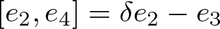


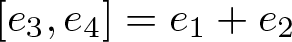
Here  $\{e_i\}$ is an orthonormal basis of the Lie algebra with
  $e_3$ timelike.
(i) The underlying Lie algebra in case (i) is
$\mathfrak{r}'_{4,\eta,\delta}$. The soliton constant is
$\boldsymbol{\mu} = -\eta^2-2\delta^2+2$ so that they can be expanding, steady or shrinking depending on the values of
$(\eta,\delta)$. They are steady if
$\eta^2+2\delta^2=2$, shrinking solitons if
$\eta^2+2\delta^2 \lt 2$, and expanding algebraic Ricci solitons otherwise. Moreover, metrics in this family are
$\mathcal{F}[t]$-critical with zero energy for
$t=-\frac{\eta^2+2\delta^2-2}{2(\eta^2+3\delta^2+2\eta\delta-1)}\in\mathbb{R}$ if the scalar curvature
$\tau=-2((\eta+\delta)^2+2\delta^2-1)$ does not vanish, and
$\mathcal{S}$-critical if and only if the scalar curvature vanishes, in which case
$\|\rho\|=0$. This family provides
$\mathcal{F}[t]$-critical metrics with zero energy for all values of
$t\in\mathbb{R}$ (as it occurs with plane waves) without having vanishing scalar curvature. Algebraic Ricci solitons which are
$\mathcal{F}[t]$-critical are steady if
$t=0$, expanding if
$-1\leq t \lt 0$, and shrinking if either
$t\leq -1$ or
$t \gt 0$.(ii) The underlying Lie algebra is
$\mathfrak{n}_4$ in case (ii) above. The algebraic Ricci soliton is shrinking with soliton constant
$\boldsymbol{\mu} = 3$, and the scalar curvature is
$\tau=2$. Moreover, this metric is
$\mathcal{F}[t]$-critical with zero energy for
$t=-\frac{3}{2}$.


Proof. A straightforward calculation shows that the components of the Ricci tensor of metrics (3),  $\rho_{ij}=\rho(e_i,e_j)$, are determined by
 \begin{equation*}
\begin{array}{lll}
\rho_{11} = - (\eta + 2 \delta) \eta ,
&
\rho_{12} = -(\eta - \delta) \gamma_1 - \nu \gamma_2 ,
&
\rho_{13} = -(\eta - \delta) \gamma_2 + \nu \gamma_1 ,
\\
\rho_{22} = - (\eta + 2 \delta) \delta - 2 \nu \gamma_3 ,
&
\rho_{23} = -(\eta + 2 \delta) \nu ,
&
\rho_{33} = (\eta + 2 \delta) \delta - 2 \nu \gamma_3 ,
\\
\rho_{44} = -\eta^2 - 2 \delta^2 + 2 \nu^2 ,
\end{array}
\end{equation*}
\begin{equation*}
\begin{array}{lll}
\rho_{11} = - (\eta + 2 \delta) \eta ,
&
\rho_{12} = -(\eta - \delta) \gamma_1 - \nu \gamma_2 ,
&
\rho_{13} = -(\eta - \delta) \gamma_2 + \nu \gamma_1 ,
\\
\rho_{22} = - (\eta + 2 \delta) \delta - 2 \nu \gamma_3 ,
&
\rho_{23} = -(\eta + 2 \delta) \nu ,
&
\rho_{33} = (\eta + 2 \delta) \delta - 2 \nu \gamma_3 ,
\\
\rho_{44} = -\eta^2 - 2 \delta^2 + 2 \nu^2 ,
\end{array}
\end{equation*}and a metric (3) is Einstein (indeed Ricci-flat) if and only if 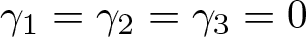 $\gamma_1=\gamma_2=\gamma_3=0$ and
  $\eta=-2\delta=\pm \frac{2}{\sqrt{3}}\nu$. Moreover, the conditions for
  $\mathfrak{D}=\operatorname{Ric}-\boldsymbol{\mu}\operatorname{Id}$ to be a derivation are determined by a system of polynomial equations on the soliton constant
  $\boldsymbol{\mu}$ and the structure constants in (3), given by
 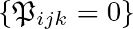 $\{\mathfrak{P}_{ijk}=0\}$, where
 \begin{align*}
\mathfrak{P}_{141} &=
(\eta - \delta) (2 \gamma_1^2 - 2 \gamma_2^2) +
4 \nu \gamma_1 \gamma_2 + (\eta^2 +
2 \delta^2 - 2 \nu^2 + \boldsymbol{\mu}) \eta ,\\
\mathfrak{P}_{142} &=
3 \nu \gamma_1 \gamma_3 - (\eta - \delta)
\gamma_2 \gamma_3 - (3 \eta^2 + \delta^2 - \eta \delta - 3 \nu^2 + \boldsymbol{\mu}) \gamma_1 -
3 \eta \nu \gamma_2 ,\\
\mathfrak{P}_{143} &=
(\eta - \delta) \gamma_1 \gamma_3 +
3 \nu \gamma_2 \gamma_3 -
3 \eta \nu \gamma_1 + (3 \eta^2 + \delta^2 - \eta \delta -
3 \nu^2 + \boldsymbol{\mu}) \gamma_2 ,\\
\mathfrak{P}_{241} &=
3 \nu \gamma_1 \gamma_3 - (\eta - \delta)
\gamma_2 \gamma_3 + (\eta^2 + 5 \delta^2 -
3 \eta \delta -
3 \nu^2 + \boldsymbol{\mu}) \gamma_1 + (\eta -
4 \delta) \nu \gamma_2 ,\\
\mathfrak{P}_{242} &=
- 2 \gamma_1^2 (\eta - \delta) -
2 \nu \gamma_1 \gamma_2 -
2 (\eta +
2 \delta) \nu \gamma_3 + (\eta^2 +
2 \delta^2 -
2 \nu^2 + \boldsymbol{\mu}) \delta ,\\
\mathfrak{P}_{243} &=
-\nu (\gamma_1^2 - \gamma_2^2 - 4 \gamma_3^2) +
2 (\eta - \delta) \gamma_1 \gamma_2
+ (\eta^2 + 2 \delta^2 - 6 \nu^2 + \boldsymbol{\mu}) (\gamma_3 -\nu)
-4\nu^3 , \\
\mathfrak{P}_{341} &=
-(\eta - \delta) \gamma_1 \gamma_3 -
3 \nu \gamma_2 \gamma_3 - (\eta -
4 \delta) \nu \gamma_1 + (\eta^2 +
5 \delta^2 - 3 \eta \delta -
3 \nu^2 + \boldsymbol{\mu}) \gamma_2 ,\\
\mathfrak{P}_{342} &=
\nu (\gamma_1^2 - \gamma_2^2 - 4 \gamma_3^2 ) -
2 (\eta - \delta) \gamma_1 \gamma_2
+ (\eta^2 + 2 \delta^2 - 6 \nu^2 + \boldsymbol{\mu}) (\gamma_3+\nu)
+4\nu^3 , \\
\mathfrak{P}_{343}& =
2 (\eta - \delta) \gamma_2^2 -
2 \nu \gamma_1 \gamma_2 +
2 (\eta +
2 \delta) \nu \gamma_3 + (\eta^2 +
2 \delta^2 -
2 \nu^2 + \boldsymbol{\mu}) \delta .
\end{align*}
\begin{align*}
\mathfrak{P}_{141} &=
(\eta - \delta) (2 \gamma_1^2 - 2 \gamma_2^2) +
4 \nu \gamma_1 \gamma_2 + (\eta^2 +
2 \delta^2 - 2 \nu^2 + \boldsymbol{\mu}) \eta ,\\
\mathfrak{P}_{142} &=
3 \nu \gamma_1 \gamma_3 - (\eta - \delta)
\gamma_2 \gamma_3 - (3 \eta^2 + \delta^2 - \eta \delta - 3 \nu^2 + \boldsymbol{\mu}) \gamma_1 -
3 \eta \nu \gamma_2 ,\\
\mathfrak{P}_{143} &=
(\eta - \delta) \gamma_1 \gamma_3 +
3 \nu \gamma_2 \gamma_3 -
3 \eta \nu \gamma_1 + (3 \eta^2 + \delta^2 - \eta \delta -
3 \nu^2 + \boldsymbol{\mu}) \gamma_2 ,\\
\mathfrak{P}_{241} &=
3 \nu \gamma_1 \gamma_3 - (\eta - \delta)
\gamma_2 \gamma_3 + (\eta^2 + 5 \delta^2 -
3 \eta \delta -
3 \nu^2 + \boldsymbol{\mu}) \gamma_1 + (\eta -
4 \delta) \nu \gamma_2 ,\\
\mathfrak{P}_{242} &=
- 2 \gamma_1^2 (\eta - \delta) -
2 \nu \gamma_1 \gamma_2 -
2 (\eta +
2 \delta) \nu \gamma_3 + (\eta^2 +
2 \delta^2 -
2 \nu^2 + \boldsymbol{\mu}) \delta ,\\
\mathfrak{P}_{243} &=
-\nu (\gamma_1^2 - \gamma_2^2 - 4 \gamma_3^2) +
2 (\eta - \delta) \gamma_1 \gamma_2
+ (\eta^2 + 2 \delta^2 - 6 \nu^2 + \boldsymbol{\mu}) (\gamma_3 -\nu)
-4\nu^3 , \\
\mathfrak{P}_{341} &=
-(\eta - \delta) \gamma_1 \gamma_3 -
3 \nu \gamma_2 \gamma_3 - (\eta -
4 \delta) \nu \gamma_1 + (\eta^2 +
5 \delta^2 - 3 \eta \delta -
3 \nu^2 + \boldsymbol{\mu}) \gamma_2 ,\\
\mathfrak{P}_{342} &=
\nu (\gamma_1^2 - \gamma_2^2 - 4 \gamma_3^2 ) -
2 (\eta - \delta) \gamma_1 \gamma_2
+ (\eta^2 + 2 \delta^2 - 6 \nu^2 + \boldsymbol{\mu}) (\gamma_3+\nu)
+4\nu^3 , \\
\mathfrak{P}_{343}& =
2 (\eta - \delta) \gamma_2^2 -
2 \nu \gamma_1 \gamma_2 +
2 (\eta +
2 \delta) \nu \gamma_3 + (\eta^2 +
2 \delta^2 -
2 \nu^2 + \boldsymbol{\mu}) \delta .
\end{align*} Since  $\nu\neq0$, we may assume
  $\nu=1$ in the rest of the proof, working in the homothetic class of the initial metric, just taking the orthogonal basis
  $\hat e_i=\frac{1}{\nu}e_i$. We start considering the ideal
  $\langle \mathfrak{P}_{ijk}\cup \{\nu-1\}\rangle$ in the polynomial ring
  $\mathbb{R}[\boldsymbol{\mu},\eta,\delta,\gamma_1,\gamma_2,\gamma_3,\nu]$. Computing a Gröbner basis of this ideal with respect to the graded reverse lexicographical order, we obtain a set of
  $35$ polynomials containing
 \begin{equation*}
\begin{array}{lll}
\boldsymbol{g}_1 = (\gamma_1^2+\gamma_2^2)\eta,
&
\boldsymbol{g}_2 = (\gamma_1^2+\gamma_2^2)\delta,
&
\boldsymbol{g}_3 = (\gamma_1^2+\gamma_2^2)(\boldsymbol{\mu}-3),
\\[0.05in]
\boldsymbol{g}_4 = (\gamma_1^2+\gamma_2^2)\gamma_1\gamma_2,
&
\boldsymbol{g}_5 = (\gamma_1^2+\gamma_2^2)(\gamma_1^2-\gamma_2^2+1),
&
\boldsymbol{g}_6 = \gamma_2\gamma_3(\boldsymbol{\mu}-12).
\end{array}
\end{equation*}
\begin{equation*}
\begin{array}{lll}
\boldsymbol{g}_1 = (\gamma_1^2+\gamma_2^2)\eta,
&
\boldsymbol{g}_2 = (\gamma_1^2+\gamma_2^2)\delta,
&
\boldsymbol{g}_3 = (\gamma_1^2+\gamma_2^2)(\boldsymbol{\mu}-3),
\\[0.05in]
\boldsymbol{g}_4 = (\gamma_1^2+\gamma_2^2)\gamma_1\gamma_2,
&
\boldsymbol{g}_5 = (\gamma_1^2+\gamma_2^2)(\gamma_1^2-\gamma_2^2+1),
&
\boldsymbol{g}_6 = \gamma_2\gamma_3(\boldsymbol{\mu}-12).
\end{array}
\end{equation*} Hence, either  $\gamma_1=\gamma_2=0$ or, otherwise,
  $\eta=\delta=\gamma_1=\gamma_3=0$,
  $\boldsymbol{\mu}=3$, and
  $\gamma_2=\varepsilon$, with
  $\varepsilon^2=1$. Next, we analyse these two cases separately.
Case 1:  $\boldsymbol{\gamma_1=\gamma_2=0}$ In this case, we have
 \begin{equation*}
\mathfrak{P}_{141} = \eta(\eta^2+2\delta^2-2+\boldsymbol{\mu}).
\end{equation*}
\begin{equation*}
\mathfrak{P}_{141} = \eta(\eta^2+2\delta^2-2+\boldsymbol{\mu}).
\end{equation*} If  $\eta=0$ then the left-invariant metric is given by
 \begin{equation*}
[e_2,e_4] = \delta e_2 +(\gamma_3-1)e_3,\quad
[e_3,e_4] = (\gamma_3+1)e_2+\delta e_3,
\end{equation*}
\begin{equation*}
[e_2,e_4] = \delta e_2 +(\gamma_3-1)e_3,\quad
[e_3,e_4] = (\gamma_3+1)e_2+\delta e_3,
\end{equation*}which corresponds to a product Lie algebra  $\mathfrak{k}\times\mathbb{R}$, with
  $\mathfrak{k}=\operatorname{span}\{e_2,e_3,e_4\}$. Since
  $e_1$ is spacelike and orthogonal to
  $\mathfrak{k}$, the Lorentzian Lie group splits as a Lorentzian product Lie group, so it does not provide any strict algebraic Ricci soliton.
Now, if  $\eta\neq0$ then
  $\boldsymbol{\mu}=-\eta^2-2\delta^2+2$, and the system
  $\{\mathfrak{P}_{ijk}=0\}$ reduces to
 \begin{equation*}
\mathfrak{P}_{243} = 4(\gamma_3-1)\gamma_3=0,\,
\mathfrak{P}_{342} = -4(\gamma_3+1)\gamma_3=0,\,
\mathfrak{P}_{343} = - \mathfrak{P}_{242} = 2(\eta+2\delta)\gamma_3=0 .
\end{equation*}
\begin{equation*}
\mathfrak{P}_{243} = 4(\gamma_3-1)\gamma_3=0,\,
\mathfrak{P}_{342} = -4(\gamma_3+1)\gamma_3=0,\,
\mathfrak{P}_{343} = - \mathfrak{P}_{242} = 2(\eta+2\delta)\gamma_3=0 .
\end{equation*} Thus,  $\gamma_3=0$, and we get an algebraic Ricci soliton with associated left-invariant metric given by
 \begin{equation*}
[e_1,e_4] = \eta e_1,\quad
[e_2,e_4] = \delta e_2-e_3,\quad
[e_3,e_4] = e_2+\delta e_3.
\end{equation*}
\begin{equation*}
[e_1,e_4] = \eta e_1,\quad
[e_2,e_4] = \delta e_2-e_3,\quad
[e_3,e_4] = e_2+\delta e_3.
\end{equation*} Since this space is Einstein if and only if  $\eta=-2\delta=\pm\frac{2}{\sqrt{3}}$, case (i) in Theorem 4.7 is obtained.
Case 2:  $\boldsymbol{\eta=\delta=\gamma_1=\gamma_3=0}, \boldsymbol{{\mu}=3}$, and
  $\boldsymbol{\gamma_2=\varepsilon}$, with
  $\boldsymbol{\varepsilon^2=1.}$ With these assumptions, the system
  $\{\mathfrak{P}_{ijk}=0\}$ is satisfied, so that we obtain an algebraic Ricci soliton with associated left-invariant metric given by
 \begin{equation*}
[e_1,e_4] = \varepsilon e_3,\quad
[e_2,e_4] = -e_3,\quad
[e_3,e_4] = \varepsilon e_1+e_2.
\end{equation*}
\begin{equation*}
[e_1,e_4] = \varepsilon e_3,\quad
[e_2,e_4] = -e_3,\quad
[e_3,e_4] = \varepsilon e_1+e_2.
\end{equation*} Note that using the isometry  $e_1\mapsto -e_1$ one may interchange the sign of
  $\varepsilon$, so we may assume
  $\varepsilon=1$, and case (ii) Theorem 4.7 is obtained, finishing the proof.
4.2.3. The minimal polynomial of the self-adjoint part of the derivation
${D_{sad}}$ has a double root

In this case, there exists a basis  $\{u_1,u_2,u_3\}$ of
  $\mathbb{R}^3$, with
  $\langle u_1,u_2\rangle=\langle u_3,u_3\rangle=1$, so that
 \begin{equation*}
D_{sad}=\left(
\begin{array}{ccc}
\eta_1 & 0 & 0
\\
\varepsilon & \eta_1 & 0
\\
0 & 0 & \eta_2
\end{array}
\right),
\quad
D_{asad}=\left(
\begin{array}{ccc}
\gamma_1 & 0 & \gamma_2
\\
0 & -\gamma_1 & \gamma_3
\\
-\gamma_3 & -\gamma_2 & 0
\end{array}
\right),
\end{equation*}
\begin{equation*}
D_{sad}=\left(
\begin{array}{ccc}
\eta_1 & 0 & 0
\\
\varepsilon & \eta_1 & 0
\\
0 & 0 & \eta_2
\end{array}
\right),
\quad
D_{asad}=\left(
\begin{array}{ccc}
\gamma_1 & 0 & \gamma_2
\\
0 & -\gamma_1 & \gamma_3
\\
-\gamma_3 & -\gamma_2 & 0
\end{array}
\right),
\end{equation*}where  $\varepsilon^2=1$. Thus, the corresponding left-invariant metrics are described by
 \begin{equation}
\mathfrak{g}_{L.II}
\left\{\!\!\!
\begin{array}{l}
{}[u_1,u_4]=(\eta_1+\gamma_1) u_1 + \varepsilon u_2 - \gamma_3 u_3, \,\,\,\,\,
{}[u_2,u_4]= (\eta_1-\gamma_1) u_2 - \gamma_2 u_3,
\\
{}[u_3,u_4]=\gamma_2 u_1+\gamma_3 u_2 + \eta_2 u_3 ,
\end{array}
\right.
\end{equation}
\begin{equation}
\mathfrak{g}_{L.II}
\left\{\!\!\!
\begin{array}{l}
{}[u_1,u_4]=(\eta_1+\gamma_1) u_1 + \varepsilon u_2 - \gamma_3 u_3, \,\,\,\,\,
{}[u_2,u_4]= (\eta_1-\gamma_1) u_2 - \gamma_2 u_3,
\\
{}[u_3,u_4]=\gamma_2 u_1+\gamma_3 u_2 + \eta_2 u_3 ,
\end{array}
\right.
\end{equation}where  $\{u_1,u_2,u_3,u_4\}$ is a basis with
  $\langle u_1,u_2\rangle=\langle u_3,u_3\rangle=\langle u_4,u_4\rangle=1$.
Theorem 4.9. A left-invariant metric  $\mathfrak{g}_{L.II}$ on
  $\mathbb{R}^3\rtimes\mathbb{R}$ given by Equation (4) is a strict algebraic Ricci soliton if and only if it is isomorphically homothetic to one of the following:
(i)
$[u_1,u_4] = \eta_1 u_1+ u_2$,
$[u_2,u_4] = \eta_1 u_2$,
$[u_3,u_4] = \eta_2 u_3$,
$\eta_2\neq 0$.(ii)
$[u_1,u_4] = -\tfrac{\eta_2}{2}u_1+ u_2$,
$[u_2,u_4] = \tfrac{4\eta_1+\eta_2}{2} u_2$,
$[u_3,u_4] = \eta_2 u_3$,with
$\eta_2(\eta_2-\eta_1)(\eta_2+2\eta_1)\neq 0$.(iii)
$[u_1,u_4] = \eta_1 u_1+ u_2-\gamma_3 u_3$,
$[u_2,u_4] = \eta_1 u_2$,
$[u_3,u_4] = \gamma_3 u_2 +\eta_1 u_3$,
$\eta_1\gamma_3\neq 0$.


Here  $\{u_i\}$ is a basis with
  $\langle u_1,u_2\rangle=\langle u_3,u_3\rangle=\langle u_4,u_4\rangle=1$.
(i) The Lie algebra is
$\mathfrak{r}_{4,\lambda}$ with
$\lambda=\frac{\eta_1}{\eta_2}$. The algebraic Ricci solitons are expanding with
$\boldsymbol{\mu} = -(2\eta_1^2+\eta_2^2)$ and
$\tau=-2(3\eta_1^2+\eta_2^2+2\eta_1\eta_2) \lt 0$. Moreover, these metrics are
$\mathcal{F}[t]$-critical with zero energy for
$t=-\frac{2\eta_1^2+\eta_2^2}{2(3\eta_1^2+\eta_2^2+2\eta_1\eta_2)}
\in [-1,-\frac{1}{4}]$.(ii) In this case, the underlying Lie algebra is
$\mathfrak{r}_{4,-2,\lambda}$ with
$\lambda=-\tfrac{4\eta_1+\eta_2}{\eta_2}$, which reduces to the product
$\mathfrak{r}_{3,-2}\times\mathbb{R}$ if
$4\eta_1+\eta_2=0$. However, the left-invariant metric is not the product one in the latter case. The algebraic Ricci solitons are expanding with soliton constant
$\boldsymbol{\mu} = -(2\eta_1^2+\eta_2^2)$ and
$\tau=-2(3\eta_1^2+\eta_2^2+2\eta_1\eta_2) \lt 0$. Moreover, these metrics are
$\mathcal{F}[t]$-critical with zero energy for
$t=-\frac{2\eta_1^2+\eta_2^2}{2(3\eta_1^2+\eta_2^2+2\eta_1\eta_2)}
\in(-1,-\frac{1}{4})$.(iii) The underlying Lie algebra is
$\mathfrak{r}_4$ and the algebraic Ricci solitons are expanding with
$\boldsymbol{\mu} = -3\eta_1^2$ and
$\tau=-12\eta_1^2$. Moreover, they are
$\mathcal{F}[-1/4]$-critical with zero energy. Furthermore, it follows from [Reference Kulkarni30] that left-invariant metrics in (iii) are homothetic (although not isomorphically homothetic) to the corresponding left-invariant metrics with
$\gamma_3=0$, and hence left-invariant metrics in case (iii) are homothetic to those in case (i) with
$\eta_2=\eta_1$.


Proof. A straightforward calculation shows that the components of the Ricci tensor of any metric (4),  $\rho_{ij}=\rho(u_i,u_j)$, are determined by
 \begin{equation*}
\begin{array}{lll}
\rho_{11} = -\varepsilon (2 \gamma_1 + 2 \eta_1 + \eta_2) ,
&
\rho_{12} = - (2 \eta_1 + \eta_2) \eta_1 ,
&
\rho_{13} = -\varepsilon \gamma_2 - (\eta_1 - \eta_2) \gamma_3 ,
\\
\rho_{23} = -(\eta_1 - \eta_2) \gamma_2 ,
&
\rho_{33} = - (2 \eta_1 + \eta_2) \eta_2 ,
&
\rho_{44} = -2 \eta_1^2 - \eta_2^2 ,
\end{array}
\end{equation*}
\begin{equation*}
\begin{array}{lll}
\rho_{11} = -\varepsilon (2 \gamma_1 + 2 \eta_1 + \eta_2) ,
&
\rho_{12} = - (2 \eta_1 + \eta_2) \eta_1 ,
&
\rho_{13} = -\varepsilon \gamma_2 - (\eta_1 - \eta_2) \gamma_3 ,
\\
\rho_{23} = -(\eta_1 - \eta_2) \gamma_2 ,
&
\rho_{33} = - (2 \eta_1 + \eta_2) \eta_2 ,
&
\rho_{44} = -2 \eta_1^2 - \eta_2^2 ,
\end{array}
\end{equation*}and a metric (4) is Einstein if and only if  $\eta_2=\eta_1$,
  $\gamma_1=-\frac{3}{2}\eta_1$ and
  $\gamma_2=0$. Moreover, the conditions for
  $\mathfrak{D}=\operatorname{Ric}-\boldsymbol{\mu}\operatorname{Id}$ to be a derivation are determined by a system of polynomial equations,
  $\{\mathfrak{P}_{ijk}=0\}$, on the soliton constant
  $\boldsymbol{\mu}$ and the structure constants in (4), where
 \begin{align*}
\mathfrak{P}_{141} &=
\varepsilon \gamma_2^2 +
2 (\eta_1 - \eta_2) \gamma_2 \gamma_3 + (2 \eta_1^2 +
\eta_2^2 + \boldsymbol{\mu}) ( \gamma_1+\eta_1) ,\\
\mathfrak{P}_{142} &=
-4 \varepsilon \gamma_1^2 +
2 (\eta_1 - \eta_2) \gamma_3^2 +
2 \varepsilon \gamma_2 \gamma_3 -
2 \varepsilon (2 \eta_1 + \eta_2) \gamma_1 + \varepsilon (2 \eta_1^2 + \eta_2^2 + \boldsymbol{\mu}) ,\\
\mathfrak{P}_{143} &=
-3 \varepsilon \gamma_1 \gamma_2 - (\eta_1 - \eta_2)
\gamma_1 \gamma_3 - \varepsilon (4 \eta_1 - \eta_2)
\gamma_2 - (5 \eta_1^2 + \eta_2^2 -
3 \eta_1 \eta_2 + \boldsymbol{\mu}) \gamma_3 ,\\
\mathfrak{P}_{241} &=
2 (\eta_1 - \eta_2) \gamma_2^2 ,\\
\mathfrak{P}_{242}& =
\varepsilon \gamma_2^2 +
2 (\eta_1 - \eta_2) \gamma_2 \gamma_3 - (\gamma_1 - \eta_1) (2 \eta_1^2 + \eta_2^2 + \boldsymbol{\mu}) ,\\
\mathfrak{P}_{243} &=
\left( (\eta_1 - \eta_2) \gamma_1 - 5 \eta_1^2 - \eta_2^2 +
3 \eta_1 \eta_2 - \boldsymbol{\mu} \right) \gamma_2 ,\\
\mathfrak{P}_{341} &=
\left( (\eta_1 - \eta_2) (\gamma_1 + \eta_1) +
3 \eta_2^2 + \boldsymbol{\mu} \right) \gamma_2 ,\\
\mathfrak{P}_{342} &=
-3 \varepsilon \gamma_1 \gamma_2 - (\eta_1 - \eta_2)
\gamma_1 \gamma_3 -
3 \varepsilon \eta_2 \gamma_2 + (\eta_1^2 +
3 \eta_2^2 - \eta_1 \eta_2 + \boldsymbol{\mu}) \gamma_3 ,\\
\mathfrak{P}_{343} &=
-2 \varepsilon \gamma_2^2 -
4 (\eta_1 - \eta_2) \gamma_2 \gamma_3 + (2 \eta_1^2 +
\eta_2^2 + \boldsymbol{\mu}) \eta_2 .
\end{align*}
\begin{align*}
\mathfrak{P}_{141} &=
\varepsilon \gamma_2^2 +
2 (\eta_1 - \eta_2) \gamma_2 \gamma_3 + (2 \eta_1^2 +
\eta_2^2 + \boldsymbol{\mu}) ( \gamma_1+\eta_1) ,\\
\mathfrak{P}_{142} &=
-4 \varepsilon \gamma_1^2 +
2 (\eta_1 - \eta_2) \gamma_3^2 +
2 \varepsilon \gamma_2 \gamma_3 -
2 \varepsilon (2 \eta_1 + \eta_2) \gamma_1 + \varepsilon (2 \eta_1^2 + \eta_2^2 + \boldsymbol{\mu}) ,\\
\mathfrak{P}_{143} &=
-3 \varepsilon \gamma_1 \gamma_2 - (\eta_1 - \eta_2)
\gamma_1 \gamma_3 - \varepsilon (4 \eta_1 - \eta_2)
\gamma_2 - (5 \eta_1^2 + \eta_2^2 -
3 \eta_1 \eta_2 + \boldsymbol{\mu}) \gamma_3 ,\\
\mathfrak{P}_{241} &=
2 (\eta_1 - \eta_2) \gamma_2^2 ,\\
\mathfrak{P}_{242}& =
\varepsilon \gamma_2^2 +
2 (\eta_1 - \eta_2) \gamma_2 \gamma_3 - (\gamma_1 - \eta_1) (2 \eta_1^2 + \eta_2^2 + \boldsymbol{\mu}) ,\\
\mathfrak{P}_{243} &=
\left( (\eta_1 - \eta_2) \gamma_1 - 5 \eta_1^2 - \eta_2^2 +
3 \eta_1 \eta_2 - \boldsymbol{\mu} \right) \gamma_2 ,\\
\mathfrak{P}_{341} &=
\left( (\eta_1 - \eta_2) (\gamma_1 + \eta_1) +
3 \eta_2^2 + \boldsymbol{\mu} \right) \gamma_2 ,\\
\mathfrak{P}_{342} &=
-3 \varepsilon \gamma_1 \gamma_2 - (\eta_1 - \eta_2)
\gamma_1 \gamma_3 -
3 \varepsilon \eta_2 \gamma_2 + (\eta_1^2 +
3 \eta_2^2 - \eta_1 \eta_2 + \boldsymbol{\mu}) \gamma_3 ,\\
\mathfrak{P}_{343} &=
-2 \varepsilon \gamma_2^2 -
4 (\eta_1 - \eta_2) \gamma_2 \gamma_3 + (2 \eta_1^2 +
\eta_2^2 + \boldsymbol{\mu}) \eta_2 .
\end{align*} First of all, note that if  $\gamma_2\neq 0$, then
  $\mathfrak{P}_{241}=0$ implies
  $\eta_2=\eta_1$. Now, a direct calculation shows that
  $\mathfrak{P}_{242}+\frac{\gamma_1-\eta_1}{\gamma_2}\mathfrak{P}_{341}=\varepsilon \gamma_2^2$, which does not vanish. Hence, necessarily
  $\gamma_2=0$.
Assuming  $\gamma_2=0$, we compute
 \begin{equation*}
\begin{array}{l}
\mathfrak{P}_{141} = (\eta_1+\gamma_1)(2\eta_1^2+\eta_2^2+\boldsymbol{\mu}),
\\[0.05in]
\mathfrak{P}_{242} = (\eta_1-\gamma_1)(2\eta_1^2+\eta_2^2+\boldsymbol{\mu}),
\\[0.05in]
\mathfrak{P}_{343} = \eta_2(2\eta_1^2+\eta_2^2+\boldsymbol{\mu}).
\end{array}
\end{equation*}
\begin{equation*}
\begin{array}{l}
\mathfrak{P}_{141} = (\eta_1+\gamma_1)(2\eta_1^2+\eta_2^2+\boldsymbol{\mu}),
\\[0.05in]
\mathfrak{P}_{242} = (\eta_1-\gamma_1)(2\eta_1^2+\eta_2^2+\boldsymbol{\mu}),
\\[0.05in]
\mathfrak{P}_{343} = \eta_2(2\eta_1^2+\eta_2^2+\boldsymbol{\mu}).
\end{array}
\end{equation*} If  $2\eta_1^2+\eta_2^2+\boldsymbol{\mu}\neq 0$, then
  $\eta_1=\eta_2=\gamma_1=0$ and the space is Einstein. Hence,
  $\boldsymbol{\mu} = -2\eta_1^2-\eta_2^2$ and the system
  $\{\mathfrak{P}_{ijk}=0\}$ reduces to
 \begin{equation}
\begin{array}{l}
\mathfrak{P}_{142} = 2(\eta_1-\eta_2)\gamma_3^2 - 2\varepsilon (2\eta_1+\eta_2+2\gamma_1) \gamma_1=0,
\\[0.05in]
\mathfrak{P}_{143} = - (\eta_1-\eta_2)(3\eta_1+\gamma_1)\gamma_3 =0,
\\[0.05in]
\mathfrak{P}_{342} = -(\eta_1-\eta_2)(\eta_1+2\eta_2+\gamma_1)\gamma_3 =0.
\end{array}
\end{equation}
\begin{equation}
\begin{array}{l}
\mathfrak{P}_{142} = 2(\eta_1-\eta_2)\gamma_3^2 - 2\varepsilon (2\eta_1+\eta_2+2\gamma_1) \gamma_1=0,
\\[0.05in]
\mathfrak{P}_{143} = - (\eta_1-\eta_2)(3\eta_1+\gamma_1)\gamma_3 =0,
\\[0.05in]
\mathfrak{P}_{342} = -(\eta_1-\eta_2)(\eta_1+2\eta_2+\gamma_1)\gamma_3 =0.
\end{array}
\end{equation} Next, we consider the cases  $\gamma_3=0$ and
  $\eta_2=\eta_1$, which we analyse separately.
Case 1:  $\boldsymbol{{\gamma_2=0}, {\mu} = -2\eta_1^2-\eta_2^2, {\gamma_3=0}.}$ In this case, Equation (5) reduces to
 \begin{equation*}
(2\eta_1+\eta_2+2\gamma_1) \gamma_1=0,
\end{equation*}
\begin{equation*}
(2\eta_1+\eta_2+2\gamma_1) \gamma_1=0,
\end{equation*}so that we analyse the cases  $\gamma_1=0$ and
  $\gamma_1= -\frac{2\eta_1+\eta_2}{2}\neq 0$.
If  $\gamma_1=0$, we get an algebraic Ricci soliton with soliton constant
  $\boldsymbol{\mu} = -2\eta_1^2-\eta_2^2$ and associated left-invariant metric given by
 \begin{equation*}
[u_1,u_4] = \eta_1 u_1+\varepsilon u_2,\quad
[u_2,u_4] = \eta_1 u_2,\quad
[u_3,u_4] = \eta_2 u_3.
\end{equation*}
\begin{equation*}
[u_1,u_4] = \eta_1 u_1+\varepsilon u_2,\quad
[u_2,u_4] = \eta_1 u_2,\quad
[u_3,u_4] = \eta_2 u_3.
\end{equation*} Using the isometry $u_4\mapsto -u_4$ one may interchange the parameters
  $(\varepsilon,\eta_1,\eta_2)$ and
  $(-\varepsilon,-\eta_1,-\eta_2)$, so we may assume
  $\varepsilon=1$. This space is Einstein if and only if
  $\eta_1=\eta_2=0$.
If  $\eta_2=0$ and
  $\eta_1\neq 0$, then the underlying Lie algebra splits as a product
  $\mathfrak{k}\times\mathbb{R}$, where the subalgebra
  $\mathfrak{k}$ is spanned by
  $\{u_1,u_2,u_4\}$. Since
  $u_3$ is spacelike and orthogonal to
  $\mathfrak{k}$, the Lorentzian Lie group splits as a Lorentzian product Lie group, hence not providing strict algebraic Ricci solitons. Finally, if
  $\eta_2\neq 0$, then case (i) in Theorem 4.9 is obtained.
If  $\gamma_1= -\frac{2\eta_1+\eta_2}{2}\neq 0$, then the left-invariant metric determined by
 \begin{equation*}
[u_1,u_4] = -\tfrac{\eta_2}{2}u_1+\varepsilon u_2,\quad
[u_2,u_4] = \tfrac{4\eta_1+\eta_2}{2} u_2,\quad
[u_3,u_4] = \eta_2 u_3,
\end{equation*}
\begin{equation*}
[u_1,u_4] = -\tfrac{\eta_2}{2}u_1+\varepsilon u_2,\quad
[u_2,u_4] = \tfrac{4\eta_1+\eta_2}{2} u_2,\quad
[u_3,u_4] = \eta_2 u_3,
\end{equation*}is an algebraic Ricci soliton with soliton constant  $\boldsymbol{\mu} = -2\eta_1^2-\eta_2^2$. Exactly as in the previous case, the isometry
  $u_4\mapsto -u_4$ allows us to assume
  $\varepsilon=1$. The space is Einstein if and only if
  $\eta_1=\eta_2$, and a direct calculation shows that it is locally symmetric whenever
  $\eta_2=0$, so that we assume
  $\eta_2(\eta_2-\eta_1)\neq 0$. This corresponds to case (ii) in Theorem 4.9.
Case 2:  $\boldsymbol{{\gamma_2=0}, {{\mu} = -3\eta_1^2}, {\gamma_3\neq 0}, {\eta_2=\eta_1}.}$ Equation (5) reduces to
 \begin{equation*}
(3\eta_1+2\gamma_1)\gamma_1=0.
\end{equation*}
\begin{equation*}
(3\eta_1+2\gamma_1)\gamma_1=0.
\end{equation*} Note that if  $3\eta_1+2\gamma_1=0$, then the space is Einstein. Now, if
  $\gamma_1=0$ and
  $\eta_1\neq 0$, we obtain an algebraic Ricci soliton with soliton constant
  $\boldsymbol{\mu} = -3\eta_1^2$ and associated left-invariant metric given by
 \begin{equation*}
[u_1,u_4] = \eta_1 u_1+\varepsilon u_2-\gamma_3 u_3,\quad
[u_2,u_4] = \eta_1 u_2,\quad
[u_3,u_4] = \gamma_3 u_2 +\eta_1 u_3.
\end{equation*}
\begin{equation*}
[u_1,u_4] = \eta_1 u_1+\varepsilon u_2-\gamma_3 u_3,\quad
[u_2,u_4] = \eta_1 u_2,\quad
[u_3,u_4] = \gamma_3 u_2 +\eta_1 u_3.
\end{equation*} As in the previous cases, we can take  $\varepsilon=1$ using the isometry
  $u_4\mapsto -u_4$, hence obtaining case (iii) in Theorem 4.9, which finishes the proof.
4.2.4. The minimal polynomial of the self-adjoint part of the derivation
${D_{sad}}$ has a triple root

There exists a basis  $\{u_1$,
  $u_2$,
  $u_3\}$ of
  $\mathbb{R}^3$, with
  $\langle u_1,u_2\rangle=\langle u_3,u_3\rangle=1$, so that
 \begin{equation*}
D_{sad}=\left(
\begin{array}{ccc}
\eta & 0 & 1
\\
0 & \eta & 0
\\
0 & 1 & \eta
\end{array}
\right),
\quad
D_{asad}=\left(
\begin{array}{ccc}
\gamma_1 & 0 & \gamma_2
\\
0 & -\gamma_1 & \gamma_3
\\
-\gamma_3 & -\gamma_2 & 0
\end{array}
\right).
\end{equation*}
\begin{equation*}
D_{sad}=\left(
\begin{array}{ccc}
\eta & 0 & 1
\\
0 & \eta & 0
\\
0 & 1 & \eta
\end{array}
\right),
\quad
D_{asad}=\left(
\begin{array}{ccc}
\gamma_1 & 0 & \gamma_2
\\
0 & -\gamma_1 & \gamma_3
\\
-\gamma_3 & -\gamma_2 & 0
\end{array}
\right).
\end{equation*}Therefore, the corresponding left-invariant metrics are given by
 \begin{equation}
\mathfrak{g}_{L.III}
\left\{
\begin{array}{l}
{}[u_1,u_4]=(\eta+\gamma_1) u_1 - \gamma_3 u_3, \quad
{}[u_2,u_4]= (\eta-\gamma_1) u_2 - (\gamma_2-1) u_3,
\\
{}[u_3,u_4]=(\gamma_2+1) u_1+\gamma_3 u_2 + \eta u_3,
\end{array}
\right.
\end{equation}
\begin{equation}
\mathfrak{g}_{L.III}
\left\{
\begin{array}{l}
{}[u_1,u_4]=(\eta+\gamma_1) u_1 - \gamma_3 u_3, \quad
{}[u_2,u_4]= (\eta-\gamma_1) u_2 - (\gamma_2-1) u_3,
\\
{}[u_3,u_4]=(\gamma_2+1) u_1+\gamma_3 u_2 + \eta u_3,
\end{array}
\right.
\end{equation}where  $\{u_1,u_2,u_3, u_4\}$ is a basis of
  $\mathbb{R}^3\rtimes \mathbb{R}$, with
  $\langle u_1,u_2\rangle=\langle u_3,u_3\rangle=\langle u_4,u_4\rangle=1$.
Theorem 4.11. A left-invariant metric  $\mathfrak{g}_{L.III}$ on
  $\mathbb{R}^3\rtimes\mathbb{R}$ given by Equation (6) is a strict algebraic Ricci soliton if and only if it is isomorphically homothetic to
 \begin{align*}
[u_1,u_4]=\eta u_1,
[u_2,u_4]= \eta u_2+u_3,
[u_3,u_4]=u_1+\eta u_3,\quad
\eta\neq 0.
\end{align*}
\begin{align*}
[u_1,u_4]=\eta u_1,
[u_2,u_4]= \eta u_2+u_3,
[u_3,u_4]=u_1+\eta u_3,\quad
\eta\neq 0.
\end{align*} Here  $\{u_i\}$ is a basis with
  $\langle u_1,u_2\rangle=\langle u_3,u_3\rangle=\langle u_4,u_4\rangle=1$.
Remark 4.12. The underlying Lie algebra in this case is  $\mathfrak{r}_4$, and the corresponding algebraic Ricci solitons are expanding with
  $\boldsymbol{\mu} = -3\eta^2$ and
  $\tau=-12\eta^2$. Moreover, these metrics are
  $\mathcal{F}[-1/4]$-critical with zero energy.
Proof. A straightforward calculation shows that the components of the Ricci tensor of any metric (6),  $\rho_{ij}=\rho(u_i,u_j)$, are determined by
 \begin{equation*}
\begin{array}{lllll}
\rho_{12} = \gamma_3 - 3 \eta^2 ,
&
\rho_{22} = 2 \gamma_2 ,
&
\rho_{23} = \gamma_1 - 3 \eta ,
&
\rho_{33} = -2 \gamma_3 - 3 \eta^2 ,
&
\rho_{44} = -3 \eta^2.
\end{array}
\end{equation*}
\begin{equation*}
\begin{array}{lllll}
\rho_{12} = \gamma_3 - 3 \eta^2 ,
&
\rho_{22} = 2 \gamma_2 ,
&
\rho_{23} = \gamma_1 - 3 \eta ,
&
\rho_{33} = -2 \gamma_3 - 3 \eta^2 ,
&
\rho_{44} = -3 \eta^2.
\end{array}
\end{equation*} Hence, a metric (6) is Einstein if and only if  $\gamma_1=3\eta$ and
  $\gamma_2=\gamma_3=0$. Moreover, the conditions for
  $\mathfrak{D}=\operatorname{Ric}-\boldsymbol{\mu}\operatorname{Id}$ to be a derivation are determined by a system of polynomial equations on the soliton constant
  $\boldsymbol{\mu}$ and the structure constants in (6), given by
  $\{\mathfrak{P}_{ijk}=0\}$, where
 \begin{equation*}\begin{array}{l}{\mathfrak P}_{141}=-\gamma_1\gamma_3+(3\eta^2+\boldsymbol\mu)(\gamma_1+\eta)+3\eta\gamma_3,\;\qquad{\mathfrak P}_{143}=(3\gamma_3-3\eta^2-\boldsymbol\mu)\gamma_3,\\{\mathfrak P}_{242}=-\gamma_1\gamma_3-(3\eta^2+\boldsymbol\mu)(\gamma_1-\eta)+3\eta\gamma_3,\;\qquad\,{\mathfrak P}_{241}=-6(\gamma_1-\eta)\gamma_2,\\{\mathfrak P}_{343}=2\gamma_1\gamma_3-6\eta\gamma_3+(3\eta^2+\boldsymbol\mu)\eta,\qquad\qquad\quad\;\,\,{\mathfrak P}_{342}=(3\gamma_3+3\eta^2+\boldsymbol\mu)\gamma_3,\\{\mathfrak P}_{243}=-\gamma_1^2+5\gamma_2\gamma_3+3\eta\gamma_1-(3\eta^2+\boldsymbol\mu)\gamma_2-3\gamma_3+3\eta^2+\boldsymbol\mu,\\{\mathfrak P}_{341}=-\gamma_1^2+5\gamma_2\gamma_3+3\eta\gamma_1+(3\eta^2+\boldsymbol\mu)\gamma_2+3\gamma_3+3\eta^2+\boldsymbol\mu.\end{array}\end{equation*}
 Note that  $\mathfrak{P}_{143} + \mathfrak{P}_{342} = 6\gamma_3^2$ and therefore necessarily
  $\gamma_3=0$. Now, using this condition, we have
 \begin{equation*}
\mathfrak{P}_{141}-\mathfrak{P}_{242} = 2(3\eta^2+\boldsymbol{\mu})\gamma_1,\quad
\mathfrak{P}_{243}+\mathfrak{P}_{341} = 2(3\eta^2+\boldsymbol{\mu})-2(\gamma_1-3\eta)\gamma_1,
\end{equation*}
\begin{equation*}
\mathfrak{P}_{141}-\mathfrak{P}_{242} = 2(3\eta^2+\boldsymbol{\mu})\gamma_1,\quad
\mathfrak{P}_{243}+\mathfrak{P}_{341} = 2(3\eta^2+\boldsymbol{\mu})-2(\gamma_1-3\eta)\gamma_1,
\end{equation*}which imply that  $\boldsymbol{\mu}=-3\eta^2$, and the system
  $\{\mathfrak{P}_{ijk}=0\}$ reduces to
 \begin{equation*}
\mathfrak{P}_{241}= -6(\gamma_1-\eta)\gamma_2=0,\quad
\mathfrak{P}_{243}=\mathfrak{P}_{341}=-(\gamma_1-3\eta)\gamma_1=0 .
\end{equation*}
\begin{equation*}
\mathfrak{P}_{241}= -6(\gamma_1-\eta)\gamma_2=0,\quad
\mathfrak{P}_{243}=\mathfrak{P}_{341}=-(\gamma_1-3\eta)\gamma_1=0 .
\end{equation*} As a consequence,  $\gamma_1\gamma_2=0$, so that we must consider the case
  $\gamma_1=\gamma_2=0$, the case
  $\gamma_1=0$,
  $\gamma_2\neq 0$,
  $\eta=0$ and the case
  $\gamma_1=3\eta\neq 0$,
  $\gamma_2=0$. Since the latter case gives an Einstein space, next we analyse the other two cases separately.
Case 1:  $\boldsymbol{\gamma_3=0}$,
  $\boldsymbol{{\mu}=-3\eta^2}$,
  $\boldsymbol{\gamma_1=\gamma_2=0.}$ In this case, the left-invariant metric, determined by
 \begin{equation*}
[u_1,u_4]=\eta u_1,\quad
[u_2,u_4]= \eta u_2+u_3,\quad
[u_3,u_4]=u_1+\eta u_3,
\end{equation*}
\begin{equation*}
[u_1,u_4]=\eta u_1,\quad
[u_2,u_4]= \eta u_2+u_3,\quad
[u_3,u_4]=u_1+\eta u_3,
\end{equation*}determines an algebraic Ricci soliton with soliton constant  $\boldsymbol{\mu}=-3\eta^2$, being Einstein if and only if
  $\eta=0$, corresponding to the case in Theorem 4.11.
Case 2:  $\boldsymbol{\gamma_3=0}$,
  $\boldsymbol{{\mu}=0}$,
  $\boldsymbol{\gamma_1=0}$,
  $\boldsymbol{\gamma_2\neq 0}$,
  $\boldsymbol{\eta=0.}$ The associated left-invariant metric is a plane wave corresponding to case (b) in Section 2.1, which does not provide any strict algebraic Ricci soliton.
Remark 4.13. The non-Einstein left-invariant plane wave metrics in Case 2 above are realized on the four-dimensional nilpotent Lie groups. The underlying Lie algebra is  $\mathfrak{h}_3\times\mathbb{R}$ if
  $\gamma_2=\pm1$, and
  $\mathfrak{n}_4$ otherwise.
4.3. Semi-direct extensions with degenerate Lie group
${\mathbb{R}}^{{3}}$

Let  $\mathfrak{g}=\mathbb{R}^3\rtimes \mathbb{R}$ be a four-dimensional Lie algebra with a Lorentzian inner product
  $\langle \cdot,\cdot \rangle$ which restricts to a degenerate inner product on the subalgebra
  $\mathbb{R}^3$. In this case there exists a basis
  $\{u_1,u_2,u_3,u_4\}$ of
  $\mathfrak{g}=\mathbb{R}^3\rtimes \mathbb{R}$, with
  $\langle u_1,u_1\rangle=\langle u_2,u_2\rangle=\langle u_3,u_4\rangle=1$, possibly after rotating the vectors
  $u_1$ and
  $u_2$, so that
 \begin{equation}
\mathfrak{g}_D
\left\{
\begin{array}{l}
{}[u_1,u_4]=\gamma_1 u_1-\gamma_2 u_2 + \gamma_3 u_3, \qquad
{}[u_2,u_4]=\gamma_2 u_1+\gamma_4 u_2 + \gamma_5 u_3,
\\
{}[u_3,u_4]=\gamma_6 u_1+\gamma_7 u_2 + \gamma_8 u_3,
\end{array}
\right.
\end{equation}
\begin{equation}
\mathfrak{g}_D
\left\{
\begin{array}{l}
{}[u_1,u_4]=\gamma_1 u_1-\gamma_2 u_2 + \gamma_3 u_3, \qquad
{}[u_2,u_4]=\gamma_2 u_1+\gamma_4 u_2 + \gamma_5 u_3,
\\
{}[u_3,u_4]=\gamma_6 u_1+\gamma_7 u_2 + \gamma_8 u_3,
\end{array}
\right.
\end{equation}for certain  $\gamma_i\in\mathbb{R}$.
Theorem 4.14. No left-invariant metric  $\mathfrak{g}_{D}$ on
  $\mathbb{R}^3\rtimes\mathbb{R}$ given by Equation (7) is a strict algebraic Ricci soliton.
Proof. A straightforward calculation shows that the components of the Ricci tensor of any metric (7),  $\rho_{ij}=\rho(u_i,u_j)$, are determined by
 \begin{equation*}\begin{array}{l}\rho_{11}=-{\textstyle\frac12}\gamma_6^2,\qquad\rho_{12}=-{\textstyle\frac12}\gamma_6\gamma_7,\;\;\qquad\qquad\qquad\qquad\rho_{14}={\textstyle\frac12}(2\gamma_1\gamma_6-\gamma_2\gamma_7+\gamma_4\gamma_6),\\\rho_{22}=-{\textstyle\frac12}\gamma_7^2,\qquad\rho_{24}={\textstyle\frac12}(\gamma_1\gamma_7+\gamma_2\gamma_6+2\gamma_4\gamma_7),\;\;\quad\,\rho_{34}={\textstyle\frac12}(\gamma_6^2+\gamma_7^2),\\\rho_{44}=-\gamma_1^2-\gamma_4^2+\gamma_1\gamma_8+\gamma_4\gamma_8-\gamma_3\gamma_6-\gamma_5\gamma_7.\end{array}\end{equation*}
 Hence, a metric (7) is Einstein if and only if  $\gamma_6=\gamma_7 =0$ and
  $
\gamma_1^2 + \gamma_4^2 -
(\gamma_1 + \gamma_4) \gamma_8 = 0
$. Moreover, the conditions for
$
\gamma_1^2 + \gamma_4^2 -
(\gamma_1 + \gamma_4) \gamma_8 = 0
$. Moreover, the conditions for  $\mathfrak{D}=\operatorname{Ric}-\boldsymbol{\mu}\operatorname{Id}$ to be a derivation are determined by a system of polynomial equations,
  $\{\mathfrak{P}_{ijk}=0\}$, on the soliton constant
  $\boldsymbol{\mu}$ and the structure constants in (7), where
 \begin{align*}
\begin{array}{ll}
2\mathfrak{P}_{142} =
3 \gamma_2 \gamma_7^2 - 3 \gamma_1 \gamma_6 \gamma_7 -
2 \gamma_2 \boldsymbol{\mu} , \quad \ \qquad\qquad 2\mathfrak{P}_{341} =
- (3 \gamma_6^2 + 3 \gamma_7^2 - 2 \boldsymbol{\mu})
\gamma_6,
\\[0.05in]
2\mathfrak{P}_{241} =
-3 \gamma_2 \gamma_6^2 - 3 \gamma_4 \gamma_6 \gamma_7 +
2 \gamma_2 \boldsymbol{\mu} , \qquad\qquad\,\,\,\, 2\mathfrak{P}_{342} =
- (3 \gamma_6^2 + 3 \gamma_7^2 - 2 \boldsymbol{\mu}) \gamma_7 ,
\\[0.05in]
2\mathfrak{P}_{141} =
-(3 \gamma_1 + \gamma_4) \gamma_6^2
- \gamma_1 \gamma_7^2
+3 \gamma_2 \gamma_6 \gamma_7 +
2 \gamma_1 \boldsymbol{\mu} ,
\\[0.05in]
2\mathfrak{P}_{143} =
\gamma_3 \gamma_6^2
+ \gamma_5 \gamma_6 \gamma_7
- \gamma_2 (2 \gamma_1 +
2 \gamma_4 - \gamma_8) \gamma_7
\\[0.05in]
\phantom{2\mathfrak{P}_{143}=}
+ \left(2 \gamma_1^2 - \gamma_2^2 + \gamma_1
(\gamma_4 -
2 \gamma_8) - \gamma_4 \gamma_8\right)
\gamma_6 + 2 \gamma_3 \boldsymbol{\mu} ,
\\[0.05in]
2\mathfrak{P}_{242} =
-\gamma_4 \gamma_6^2
- (\gamma_1 + 3 \gamma_4) \gamma_7^2
-3\gamma_2 \gamma_6 \gamma_7 +
2 \gamma_4 \boldsymbol{\mu} ,
\\[0.05in]
2\mathfrak{P}_{243} =
\gamma_5 \gamma_7^2
+ \gamma_3 \gamma_6 \gamma_7
+ \gamma_2 (2 \gamma_1 + 2 \gamma_4 - \gamma_8) \gamma_6
\\[0.05in]
\phantom{2\mathfrak{P}_{243} =}
- \left(
\gamma_2^2-(\gamma_1 +
2 \gamma_4) (\gamma_4 - \gamma_8) \right)
\gamma_7 + 2 \gamma_5 \boldsymbol{\mu} ,
\\[0.05in]
2\mathfrak{P}_{343} =
(2 \gamma_1 + \gamma_4 - \gamma_8) \gamma_6^2 + (\gamma_1 +
2 \gamma_4 - \gamma_8) \gamma_7^2
+
2 \gamma_8 \boldsymbol{\mu} .
\end{array}
\end{align*}
\begin{align*}
\begin{array}{ll}
2\mathfrak{P}_{142} =
3 \gamma_2 \gamma_7^2 - 3 \gamma_1 \gamma_6 \gamma_7 -
2 \gamma_2 \boldsymbol{\mu} , \quad \ \qquad\qquad 2\mathfrak{P}_{341} =
- (3 \gamma_6^2 + 3 \gamma_7^2 - 2 \boldsymbol{\mu})
\gamma_6,
\\[0.05in]
2\mathfrak{P}_{241} =
-3 \gamma_2 \gamma_6^2 - 3 \gamma_4 \gamma_6 \gamma_7 +
2 \gamma_2 \boldsymbol{\mu} , \qquad\qquad\,\,\,\, 2\mathfrak{P}_{342} =
- (3 \gamma_6^2 + 3 \gamma_7^2 - 2 \boldsymbol{\mu}) \gamma_7 ,
\\[0.05in]
2\mathfrak{P}_{141} =
-(3 \gamma_1 + \gamma_4) \gamma_6^2
- \gamma_1 \gamma_7^2
+3 \gamma_2 \gamma_6 \gamma_7 +
2 \gamma_1 \boldsymbol{\mu} ,
\\[0.05in]
2\mathfrak{P}_{143} =
\gamma_3 \gamma_6^2
+ \gamma_5 \gamma_6 \gamma_7
- \gamma_2 (2 \gamma_1 +
2 \gamma_4 - \gamma_8) \gamma_7
\\[0.05in]
\phantom{2\mathfrak{P}_{143}=}
+ \left(2 \gamma_1^2 - \gamma_2^2 + \gamma_1
(\gamma_4 -
2 \gamma_8) - \gamma_4 \gamma_8\right)
\gamma_6 + 2 \gamma_3 \boldsymbol{\mu} ,
\\[0.05in]
2\mathfrak{P}_{242} =
-\gamma_4 \gamma_6^2
- (\gamma_1 + 3 \gamma_4) \gamma_7^2
-3\gamma_2 \gamma_6 \gamma_7 +
2 \gamma_4 \boldsymbol{\mu} ,
\\[0.05in]
2\mathfrak{P}_{243} =
\gamma_5 \gamma_7^2
+ \gamma_3 \gamma_6 \gamma_7
+ \gamma_2 (2 \gamma_1 + 2 \gamma_4 - \gamma_8) \gamma_6
\\[0.05in]
\phantom{2\mathfrak{P}_{243} =}
- \left(
\gamma_2^2-(\gamma_1 +
2 \gamma_4) (\gamma_4 - \gamma_8) \right)
\gamma_7 + 2 \gamma_5 \boldsymbol{\mu} ,
\\[0.05in]
2\mathfrak{P}_{343} =
(2 \gamma_1 + \gamma_4 - \gamma_8) \gamma_6^2 + (\gamma_1 +
2 \gamma_4 - \gamma_8) \gamma_7^2
+
2 \gamma_8 \boldsymbol{\mu} .
\end{array}
\end{align*} In view of the components above, we study the case  $\gamma_6=\gamma_7=0$, the case
  $\gamma_6=0$,
  $\gamma_7\neq 0$, and the case
  $\gamma_6\neq 0$ separately.
Case 1:  $\boldsymbol{\gamma_6=\gamma_7=0.}$ The associated left-invariant metric is a plane wave corresponding to case (c) in Section 2.1, which does not provide any strict algebraic Ricci soliton.
Case 2:  $\boldsymbol{\gamma_6=0}$,
  $\boldsymbol{\gamma_7\neq0.}$ If
  $\gamma_6=0$, we have
 \begin{equation*}
\mathfrak{P}_{342} = -\tfrac{1}{2}(3\gamma_7^2-2\boldsymbol{\mu})\gamma_7,\quad
\mathfrak{P}_{241} = \gamma_2\boldsymbol{\mu},\quad
\mathfrak{P}_{141} = -\tfrac{1}{2}(\gamma_7^2-2\boldsymbol{\mu})\gamma_1.
\end{equation*}
\begin{equation*}
\mathfrak{P}_{342} = -\tfrac{1}{2}(3\gamma_7^2-2\boldsymbol{\mu})\gamma_7,\quad
\mathfrak{P}_{241} = \gamma_2\boldsymbol{\mu},\quad
\mathfrak{P}_{141} = -\tfrac{1}{2}(\gamma_7^2-2\boldsymbol{\mu})\gamma_1.
\end{equation*} Since  $\gamma_7\neq 0$, it follows that
  $
\boldsymbol{\mu} = \tfrac{3}{2}\gamma_7^2
$ and
$
\boldsymbol{\mu} = \tfrac{3}{2}\gamma_7^2
$ and  $\gamma_1=\gamma_2=0$. Now,
 \begin{equation*}
\mathfrak{P}_{343} = (\gamma_4+\gamma_8)\gamma_7^2
\end{equation*}
\begin{equation*}
\mathfrak{P}_{343} = (\gamma_4+\gamma_8)\gamma_7^2
\end{equation*}leads to  $\gamma_8=-\gamma_4$, and the system
  $\{\mathfrak{P}_{ijk}=0\}$ reduces to
 \begin{equation*}
\mathfrak{P}_{143} = \tfrac{3}{2} \gamma_3\gamma_7^2,\quad
\mathfrak{P}_{243} = 2(\gamma_4^2+\gamma_5\gamma_7)\gamma_7.
\end{equation*}
\begin{equation*}
\mathfrak{P}_{143} = \tfrac{3}{2} \gamma_3\gamma_7^2,\quad
\mathfrak{P}_{243} = 2(\gamma_4^2+\gamma_5\gamma_7)\gamma_7.
\end{equation*} Hence,  $\gamma_3=0$ and
  $\gamma_5=-\frac{\gamma_4^2}{\gamma_7}$, and (7) becomes
 \begin{equation*}
[u_2,u_4]= \gamma_4 u_2 -\tfrac{\gamma_4^2}{\gamma_7} u_3,\quad
[u_3,u_4] = \gamma_7 u_2-\gamma_4 u_3,
\end{equation*}
\begin{equation*}
[u_2,u_4]= \gamma_4 u_2 -\tfrac{\gamma_4^2}{\gamma_7} u_3,\quad
[u_3,u_4] = \gamma_7 u_2-\gamma_4 u_3,
\end{equation*}so that the Lie algebra splits as a product  $\mathfrak{g}=\mathfrak{k}\times\mathbb{R}$ with
  $\mathfrak{k}=\operatorname{span}\{u_2,u_3,u_4\}$. Since
  $u_1$ is spacelike and orthogonal to
  $\mathfrak{k}$, the Lorentzian Lie group splits as a Lorentzian product Lie group, and this case does not provide any strict algebraic Ricci soliton.
Case 3:  $\boldsymbol{\gamma_6\neq 0}.$ Since
  $\mathfrak{P}_{341}=-\frac{1}{2}(3\gamma_6^2+3\gamma_7^2-2\boldsymbol{\mu})\gamma_6$, the soliton constant is given by
  $\boldsymbol{\mu}=\frac{3}{2}(\gamma_6^2+\gamma_7^2)$ and, as a consequence,
  $\mathfrak{P}_{142}=-\frac{3}{2}(\gamma_2\gamma_6+\gamma_1\gamma_7)\gamma_6$, so that
  $\gamma_2=-\frac{\gamma_1\gamma_7}{\gamma_6}$. Now
  $\mathfrak{P}_{141} =- \frac{1}{2}(\gamma_4\gamma_6^2+\gamma_1\gamma_7^2)$, which implies
  $\gamma_4=-\frac{\gamma_1\gamma_7^2}{\gamma_6^2}$. Next, we compute
  $\mathfrak{P}_{343}=\frac{\left( \gamma_1(\gamma_6^2-\gamma_7^2)+\gamma_6^2\gamma_8\right)(\gamma_6^2+\gamma_7^2)}{\gamma_6^2}$, which leads to
  $\gamma_8=-\frac{(\gamma_6^2-\gamma_7^2)\gamma_1}{\gamma_6^2}$. At this point, we have
 \begin{equation*}
2\gamma_6^3 \mathfrak{P}_{143} =
(4 \gamma_6^2 + 3 \gamma_7^2) \gamma_6^3 \gamma_3
+ 2 (\gamma_6^2 - \gamma_7^2) (2 \gamma_6^2 +
\gamma_7^2)\gamma_1^2
+ \gamma_5 \gamma_6^4 \gamma_7 .
\end{equation*}
\begin{equation*}
2\gamma_6^3 \mathfrak{P}_{143} =
(4 \gamma_6^2 + 3 \gamma_7^2) \gamma_6^3 \gamma_3
+ 2 (\gamma_6^2 - \gamma_7^2) (2 \gamma_6^2 +
\gamma_7^2)\gamma_1^2
+ \gamma_5 \gamma_6^4 \gamma_7 .
\end{equation*} Now, using that the coefficient of  $\gamma_3$ does not vanish, we can clear up this unknown, and using its expression, the system
  $\{\mathfrak{P}_{ijk}=0\}$ finally reduces to
 \begin{equation*}
\mathfrak{P}_{243} =
\tfrac{6\left(\gamma_5\gamma_6^4-(\gamma_6^2-\gamma_7^2)\gamma_1^2\gamma_7\right)
(\gamma_6^2+\gamma_7^2)^2}
{(4 \gamma_6^2 + 3 \gamma_7^2) \gamma_6^4},
\end{equation*}
\begin{equation*}
\mathfrak{P}_{243} =
\tfrac{6\left(\gamma_5\gamma_6^4-(\gamma_6^2-\gamma_7^2)\gamma_1^2\gamma_7\right)
(\gamma_6^2+\gamma_7^2)^2}
{(4 \gamma_6^2 + 3 \gamma_7^2) \gamma_6^4},
\end{equation*}from where  $\gamma_5=\tfrac{(\gamma_6^2-\gamma_7^2)\gamma_1^2\gamma_7}{\gamma_6^4}$. Therefore, (7) reduces to
 \begin{equation*}
\begin{array}{l}
[u_1,u_4]= \gamma_1 u_1 +\tfrac{\gamma_1\gamma_7}{\gamma_6} u_2
- \tfrac{(\gamma_6^2-\gamma_7^2)\gamma_1^2}{\gamma_6^3} u_3,
\\[0.2cm]
[u_2,u_4] = -\tfrac{\gamma_1\gamma_7}{\gamma_6} u_1
- \tfrac{\gamma_1\gamma_7^2}{\gamma_6^2} u_2
+ \tfrac{(\gamma_6^2-\gamma_7^2)\gamma_1^2\gamma_7}{\gamma_6^4}u_3 ,
\\[0.2cm]
[u_3,u_4] = \gamma_6 u_1+\gamma_7 u_2
- \tfrac{(\gamma_6^2-\gamma_7^2)\gamma_1}{\gamma_6^2} u_3,
\end{array}
\end{equation*}
\begin{equation*}
\begin{array}{l}
[u_1,u_4]= \gamma_1 u_1 +\tfrac{\gamma_1\gamma_7}{\gamma_6} u_2
- \tfrac{(\gamma_6^2-\gamma_7^2)\gamma_1^2}{\gamma_6^3} u_3,
\\[0.2cm]
[u_2,u_4] = -\tfrac{\gamma_1\gamma_7}{\gamma_6} u_1
- \tfrac{\gamma_1\gamma_7^2}{\gamma_6^2} u_2
+ \tfrac{(\gamma_6^2-\gamma_7^2)\gamma_1^2\gamma_7}{\gamma_6^4}u_3 ,
\\[0.2cm]
[u_3,u_4] = \gamma_6 u_1+\gamma_7 u_2
- \tfrac{(\gamma_6^2-\gamma_7^2)\gamma_1}{\gamma_6^2} u_3,
\end{array}
\end{equation*}which is a shrinking algebraic Ricci soliton with soliton constant  $\boldsymbol{\mu}=\frac{3}{2}(\gamma_6^2+\gamma_7^2)$. Since
  $\gamma_6(\gamma_6^2+\gamma_7^2)\neq 0$, considering the basis
 \begin{equation*}
\bar u_1=u_3,\quad \bar u_2=\gamma_6 u_1+\gamma_7 u_2,\quad \bar u_3=\gamma_6\gamma_7 u_1-\gamma_6^2 u_2-2\gamma_1\gamma_7 u_3,\quad \bar u_4=2\gamma_1\gamma_7 u_2-\gamma_6^2 u_4,
\end{equation*}
\begin{equation*}
\bar u_1=u_3,\quad \bar u_2=\gamma_6 u_1+\gamma_7 u_2,\quad \bar u_3=\gamma_6\gamma_7 u_1-\gamma_6^2 u_2-2\gamma_1\gamma_7 u_3,\quad \bar u_4=2\gamma_1\gamma_7 u_2-\gamma_6^2 u_4,
\end{equation*}one has the brackets
 \begin{equation*}
[\bar u_1,\bar u_4]=\gamma_1(\gamma_6^2-\gamma_7^2)\bar u_1 -\gamma_6^2\bar u_2,\quad
[\bar u_2,\bar u_4]=\tfrac{\gamma_1^2(\gamma_6^2-\gamma_7^2)^2}{\gamma_6^2}\bar u_1-\gamma_1(\gamma_6^2-\gamma_7^2)\bar u_2,
\end{equation*}
\begin{equation*}
[\bar u_1,\bar u_4]=\gamma_1(\gamma_6^2-\gamma_7^2)\bar u_1 -\gamma_6^2\bar u_2,\quad
[\bar u_2,\bar u_4]=\tfrac{\gamma_1^2(\gamma_6^2-\gamma_7^2)^2}{\gamma_6^2}\bar u_1-\gamma_1(\gamma_6^2-\gamma_7^2)\bar u_2,
\end{equation*}which shows that the Lie algebra splits as a product  $\mathfrak{g}=\mathfrak{k}\times\mathbb{R}$, where
  $\mathfrak{k}=\operatorname{span}\{\bar u_1,\bar u_2,\bar u_4\}$. Moreover, a straightforward calculation shows that
  $\bar u_3$ is orthogonal to
  $\mathfrak{k}$ and
  $\langle\bar u_3,\bar u_3\rangle=\gamma_6^2(\gamma_6^2+\gamma_7^2) \gt 0$. Hence, the Lorentzian Lie group is a product Lorentzian Lie group, and there are no strict algebraic Ricci solitons in this case, thus finishing the proof.
Remark 4.15. Any non-Abelian semi-direct extension  $\mathbb{R}^3\rtimes\mathbb{R}$ of the Abelian Lie group but the
  $\mathfrak{S}$-type Lie group with Lie algebra
  $\mathfrak{r}_{4,1,1}$ admits non-Einstein left-invariant Lorentz metrics which are plane waves.
The case of nilpotent extensions was already considered in Remark 4.13.
We take  $\gamma_6=\gamma_7=0$, and set
  $\xi=(\gamma_1,\gamma_2,\gamma_3,\gamma_4,\gamma_5,\gamma_8)$. The product Lie groups corresponding to
  $\mathfrak{r}_{3}\times\mathbb{R}$,
  $\mathfrak{r}_{3,\lambda}\times\mathbb{R}$, and
  $\mathfrak{r}'_{3,\lambda}\times\mathbb{R}$ admit non-Einstein left-invariant plane wave metrics given by
  $\mathfrak{g}_{D}$ for the special choice of
  $\xi=(-2,-1,1,0,0,0)$,
  $\xi=(-1,0,0,-\lambda,0,0)$, and
  $\xi=(-\lambda+1,\frac{2}{\sqrt{2}},0,-\lambda-1,0,0)$, respectively.
The Lie algebra  $\mathfrak{r}_4$ admits a non-Einstein plane-wave left-invariant metric
  $\mathfrak{g}_{D}$ determined by
  $\xi=(-2,-1,1,0,0,-1)$. The left-invariant metrics corresponding to
  $\xi=(-\lambda,0,-1,-1,0,-\lambda)$ are realized on
  $\mathfrak{r}_{4,\lambda}$ for
  $\lambda\neq1$, and
  $\xi=(-2,1,0,0,0,-1)$ realizes on
  $\mathfrak{r}_{4,1}$.
The Lie algebra  $\mathfrak{r}_{4,\mu,\lambda}$ admits left-invariant non-Einstein plane wave metrics
  $\mathfrak{g}_{D}$ determined by
  $\xi=(-1,0,0,-\mu,0,-\lambda)$ if
  $\mu^2-\lambda\mu-\lambda+1\neq0$, and
  $\xi=(-\mu,0,0,-\lambda,0,-1)$ if
  $\mu^2-\lambda\mu-\lambda+1=0$. This covers all the cases but
  $\mathfrak{r}_{4,1,1}$. The remaining Lie algebra
  $\mathfrak{r}'_{4,\mu,\lambda}$ admits left-invariant non-Einstein plane wave metrics
  $\mathfrak{g}_{D}$ determined by
  $\xi=(-\mu-2\lambda,\sqrt{(\lambda+\mu)^2+1},0,\mu,0,-\mu)$ for any value of
  $\lambda$ and
  $\mu\neq 0$.
5. Semi-direct extensions of the Heisenberg group
$\mathcal{H}^3$

We proceed as in the case of the Abelian Lie group, considering separately the cases when the induced metric on  $\mathcal{H}^3$ is positive definite, Lorentzian or degenerate. Hence, Theorem 2.6 follows at once from the analysis below.
5.1. Semi-direct extensions with Riemannian normal subgroup
$\mathcal{H}^{3}$

In this section, we consider left-invariant Lorentzian metrics which are obtained as extensions of the three-dimensional Riemannian Heisenberg Lie group  $\mathcal{H}^3$. Following Section 3.1, one may describe all such Lorentzian extensions considering a suitable orthonormal basis
  $\{e_i\}$ with
  $\mathfrak{h}_3=\operatorname{span}\{e_1,e_2,e_3\}$ and a timelike vector
  $e_4$ orthogonal to
  $\mathfrak{h}_3$ such that the symmetric part of
  $\operatorname{ad}_{e_4}$ is diagonal. Hence, the Lie brackets become
 \begin{equation}
\mathfrak{g}_R
\left\{
\begin{array}{ll}
{}[e_1,e_2]=\lambda_3 e_3, &
{}[e_1,e_4]=\gamma_1 e_1-\gamma_2 e_2 + \gamma_3 e_3,
\\
{}[e_2,e_4]=\gamma_2 e_1 + \gamma_4 e_2 + \gamma_5 e_3, &
{}[e_3,e_4]=(\gamma_1 +\gamma_4)e_3,
\end{array}
\right.
\end{equation}
\begin{equation}
\mathfrak{g}_R
\left\{
\begin{array}{ll}
{}[e_1,e_2]=\lambda_3 e_3, &
{}[e_1,e_4]=\gamma_1 e_1-\gamma_2 e_2 + \gamma_3 e_3,
\\
{}[e_2,e_4]=\gamma_2 e_1 + \gamma_4 e_2 + \gamma_5 e_3, &
{}[e_3,e_4]=(\gamma_1 +\gamma_4)e_3,
\end{array}
\right.
\end{equation}where  $\lambda_3\neq 0$ and
  $\gamma_1$,
  $\dots$,
  $\gamma_5\in\mathbb{R}$.
Remark 5.1. We introduce a parameter  $\delta$, which will be used in what follows with the purpose of facilitating the solution of the case in Section 5.2.1, proceeding exactly as in the present section. In the case at hand,
  $\delta = 1$, while in Section 5.2.1, it takes the value
  $\delta = -1$.
Considering the new basis  $\bar e_1 = e_1$,
  $\bar e_2 = e_2$,
  $\bar e_3 = e_3$,
  $\bar e_4 = \delta\tfrac{\gamma_5}{\lambda_3} e_1 - \delta\tfrac{\gamma_3}{\lambda_3} e_2 +e_4$, the Lie bracket transforms into
 \begin{equation*}
[\bar e_1,\bar e_2] = \delta \lambda_3 \bar e_3,
\,\,
[\bar e_1,\bar e_4] = \gamma_1 \bar e_1 -\gamma_2 \bar e_2,
\,\,
[\bar e_2, \bar e_4] = \gamma_2 \bar e_1 + \gamma_4 \bar e_2 ,
\,\,
[\bar e_3, \bar e_4] = (\gamma_1+\gamma_4) \bar e_3,
\end{equation*}
\begin{equation*}
[\bar e_1,\bar e_2] = \delta \lambda_3 \bar e_3,
\,\,
[\bar e_1,\bar e_4] = \gamma_1 \bar e_1 -\gamma_2 \bar e_2,
\,\,
[\bar e_2, \bar e_4] = \gamma_2 \bar e_1 + \gamma_4 \bar e_2 ,
\,\,
[\bar e_3, \bar e_4] = (\gamma_1+\gamma_4) \bar e_3,
\end{equation*}and a direct calculation shows that, when evaluating on the basis  $\{\bar e_i\}$,
 \begin{equation*}
\text{ad}_{\bar e_4}=\left(
\begin{array}{cc}
A& 0
\\
0 & \operatorname{tr}A
\end{array}
\right),
\quad \text{where}\,\,
A=\left(
\begin{array}{cc}
-\gamma_1 & -\gamma_2
\\
\gamma_2 & -\gamma_4
\end{array}
\right).
\qquad\qquad
\end{equation*}
\begin{equation*}
\text{ad}_{\bar e_4}=\left(
\begin{array}{cc}
A& 0
\\
0 & \operatorname{tr}A
\end{array}
\right),
\quad \text{where}\,\,
A=\left(
\begin{array}{cc}
-\gamma_1 & -\gamma_2
\\
\gamma_2 & -\gamma_4
\end{array}
\right).
\qquad\qquad
\end{equation*} Hence, the Lie algebra corresponds to  $ \mathfrak{h}_3\times\mathbb{R} $ or
  $\mathfrak{n}_4$ if and only if
  $\gamma_4=-\gamma_1$ and
  $\gamma_1^2=\gamma_2^2$ (cf. [Reference Andrada, Barberis, Dotti and Ovando2]).
Theorem 5.2. Any left-invariant metric  $\mathfrak{g}_R$ on
  $\mathcal{H}^3\rtimes\mathbb{R}$ given by Equation (8), which is an algebraic Ricci soliton, is also realized on
  $\mathbb{R}^3\rtimes\mathbb{R}$.
Proof. A straightforward calculation shows that the components of the Ricci tensor of any metric (8),  $\rho_{ij}=\rho(e_i,e_j)$, are determined by
 \begin{equation*}
\begin{array}{ll}
\rho_{11} = \tfrac{1}{2}\delta (4 \gamma_1^2 + \delta \gamma_3^2 +
4 \gamma_1 \gamma_4 - \lambda_3^2) ,
&
\rho_{12} = \tfrac{1}{2} (2 \delta\gamma_1 \gamma_2 -
2 \delta \gamma_2 \gamma_4 + \gamma_3 \gamma_5) ,
\\
\rho_{13} = \tfrac{1}{2} (2 \gamma_1 \gamma_3 - \gamma_2 \gamma_5 +
3 \gamma_3 \gamma_4) ,
&
\rho_{14} = \tfrac{1}{2} \gamma_5 \lambda_3 ,
\\
\rho_{22} = \tfrac{1}{2} \delta(4 \gamma_4^2 + \delta \gamma_5^2 +
4 \gamma_1 \gamma_4 - \lambda_3^2) ,
&
\rho_{23} = \tfrac{1}{2} (3 \gamma_1 \gamma_5 + \gamma_2 \gamma_3 +
2 \gamma_4 \gamma_5) ,
\\
\rho_{44} = - \tfrac{1}{2} (4 \gamma_1^2 + \delta \gamma_3^2 +
4 \gamma_4^2 + \delta \gamma_5^2 + 4 \gamma_1 \gamma_4) ,
&
\rho_{24} = -\tfrac{1}{2} \gamma_3 \lambda_3 ,
\\
\rho_{33} = \tfrac{1}{2} (4 \gamma_1^2 - \delta \gamma_3^2 + 4 \gamma_4^2 - \delta \gamma_5^2 +
8 \gamma_1 \gamma_4 + \lambda_3^2) .
\end{array}
\end{equation*}
\begin{equation*}
\begin{array}{ll}
\rho_{11} = \tfrac{1}{2}\delta (4 \gamma_1^2 + \delta \gamma_3^2 +
4 \gamma_1 \gamma_4 - \lambda_3^2) ,
&
\rho_{12} = \tfrac{1}{2} (2 \delta\gamma_1 \gamma_2 -
2 \delta \gamma_2 \gamma_4 + \gamma_3 \gamma_5) ,
\\
\rho_{13} = \tfrac{1}{2} (2 \gamma_1 \gamma_3 - \gamma_2 \gamma_5 +
3 \gamma_3 \gamma_4) ,
&
\rho_{14} = \tfrac{1}{2} \gamma_5 \lambda_3 ,
\\
\rho_{22} = \tfrac{1}{2} \delta(4 \gamma_4^2 + \delta \gamma_5^2 +
4 \gamma_1 \gamma_4 - \lambda_3^2) ,
&
\rho_{23} = \tfrac{1}{2} (3 \gamma_1 \gamma_5 + \gamma_2 \gamma_3 +
2 \gamma_4 \gamma_5) ,
\\
\rho_{44} = - \tfrac{1}{2} (4 \gamma_1^2 + \delta \gamma_3^2 +
4 \gamma_4^2 + \delta \gamma_5^2 + 4 \gamma_1 \gamma_4) ,
&
\rho_{24} = -\tfrac{1}{2} \gamma_3 \lambda_3 ,
\\
\rho_{33} = \tfrac{1}{2} (4 \gamma_1^2 - \delta \gamma_3^2 + 4 \gamma_4^2 - \delta \gamma_5^2 +
8 \gamma_1 \gamma_4 + \lambda_3^2) .
\end{array}
\end{equation*} Hence, a metric (8) is never Einstein. Moreover, the conditions for  $\mathfrak{D}=\operatorname{Ric}-\boldsymbol{\mu}\operatorname{Id}$ to be a derivation, given by a system of polynomial equations
  $\{\mathfrak{P}_{ijk}=0\}$ on the soliton constant
  $\boldsymbol{\mu}$ and the structure constants in (8), we will make use of the following polynomials:
 \begin{align*}
\begin{array}{ll}
2 \mathfrak{P}_{121} =
\delta (\gamma_1 \gamma_3 - 2 \gamma_2 \gamma_5 +
3 \gamma_3 \gamma_4) \lambda_3 , \qquad\qquad 2 \mathfrak{P}_{122} =
\delta (3 \gamma_1 \gamma_5 +
2 \gamma_2 \gamma_3 + \gamma_4 \gamma_5 ) \lambda_3,
\\[0.05in]
2 \mathfrak{P}_{123} =
- \delta (3 \gamma_3^2 + 3 \gamma_5^2 - 3 \delta \lambda_3^2 -
2 \boldsymbol{\mu}) \lambda_3 , \qquad\,\,\,\, 2 \mathfrak{P}_{144} =
- \delta (\gamma_1 \gamma_5 + \gamma_2 \gamma_3) \lambda_3 ,
\\[0.05in]
2 \mathfrak{P}_{142} =
2 \delta (5 \gamma_1^2 + \gamma_4^2) \gamma_2 +
3 \gamma_2 \gamma_3^2 + (4 \gamma_1 + \gamma_4) \gamma_3
\gamma_5 - 2 \gamma_2 \boldsymbol{\mu} ,
\\[0.05in]
2 \mathfrak{P}_{241} =
-2 \delta (\gamma_1^2 + 5 \gamma_4^2) \gamma_2
- 3 \gamma_2 \gamma_5^2 + (\gamma_1 +
4 \gamma_4 ) \gamma_3 \gamma_5 + 2 \gamma_2 \boldsymbol{\mu} ,
\\[0.05in]
2 \mathfrak{P}_{242} =
-4 \delta \left(\gamma_4^3 + \gamma_1^2 \gamma_4 - (\gamma_1 -
\gamma_4) \gamma_2^2 + \gamma_1 \gamma_4^2 \right)
- \gamma_3^2 \gamma_4
\\[0.05in]\phantom{2 \mathfrak{P}_{242} =}
+ (3 \gamma_1 + \gamma_4) \gamma_5^2 +
3 \gamma_2 \gamma_3 \gamma_5 + 2 \gamma_4 \boldsymbol{\mu},
\\[0.05in]
2\mathfrak{P}_{244} =
- \delta (\gamma_2 \gamma_5 - \gamma_3 \gamma_4) \lambda_3,
\\[0.05in]
2 \mathfrak{P}_{341} =
-\gamma_2^2 \gamma_3 -
3 (\gamma_1 + \gamma_4) \gamma_2 \gamma_5 + (2 \gamma_1 +
3 \gamma_4) \gamma_3 \gamma_4 ,
\\[0.05in]
2 \mathfrak{P}_{342} =
(3 \gamma_1^2 - \gamma_2^2) \gamma_5 +
3 ( \gamma_1 + \gamma_4) \gamma_2 \gamma_3 +
2 \gamma_1 \gamma_4 \gamma_5 ,
\\[0.05in]
2 \mathfrak{P}_{343} =
-4 \delta (\gamma_1^2 + \gamma_4^2 + \gamma_1 \gamma_4) (\gamma_1 +
\gamma_4)
- (3 \gamma_1 + 4 \gamma_4) \gamma_3^2
\\[0.05in]
\phantom{2 \mathfrak{P}_{343} =}
- (4 \gamma_1 +
3 \gamma_4 ) \gamma_5^2 + 2 (\gamma_1 + \gamma_4) \boldsymbol{\mu} .
\end{array}
\end{align*}
\begin{align*}
\begin{array}{ll}
2 \mathfrak{P}_{121} =
\delta (\gamma_1 \gamma_3 - 2 \gamma_2 \gamma_5 +
3 \gamma_3 \gamma_4) \lambda_3 , \qquad\qquad 2 \mathfrak{P}_{122} =
\delta (3 \gamma_1 \gamma_5 +
2 \gamma_2 \gamma_3 + \gamma_4 \gamma_5 ) \lambda_3,
\\[0.05in]
2 \mathfrak{P}_{123} =
- \delta (3 \gamma_3^2 + 3 \gamma_5^2 - 3 \delta \lambda_3^2 -
2 \boldsymbol{\mu}) \lambda_3 , \qquad\,\,\,\, 2 \mathfrak{P}_{144} =
- \delta (\gamma_1 \gamma_5 + \gamma_2 \gamma_3) \lambda_3 ,
\\[0.05in]
2 \mathfrak{P}_{142} =
2 \delta (5 \gamma_1^2 + \gamma_4^2) \gamma_2 +
3 \gamma_2 \gamma_3^2 + (4 \gamma_1 + \gamma_4) \gamma_3
\gamma_5 - 2 \gamma_2 \boldsymbol{\mu} ,
\\[0.05in]
2 \mathfrak{P}_{241} =
-2 \delta (\gamma_1^2 + 5 \gamma_4^2) \gamma_2
- 3 \gamma_2 \gamma_5^2 + (\gamma_1 +
4 \gamma_4 ) \gamma_3 \gamma_5 + 2 \gamma_2 \boldsymbol{\mu} ,
\\[0.05in]
2 \mathfrak{P}_{242} =
-4 \delta \left(\gamma_4^3 + \gamma_1^2 \gamma_4 - (\gamma_1 -
\gamma_4) \gamma_2^2 + \gamma_1 \gamma_4^2 \right)
- \gamma_3^2 \gamma_4
\\[0.05in]\phantom{2 \mathfrak{P}_{242} =}
+ (3 \gamma_1 + \gamma_4) \gamma_5^2 +
3 \gamma_2 \gamma_3 \gamma_5 + 2 \gamma_4 \boldsymbol{\mu},
\\[0.05in]
2\mathfrak{P}_{244} =
- \delta (\gamma_2 \gamma_5 - \gamma_3 \gamma_4) \lambda_3,
\\[0.05in]
2 \mathfrak{P}_{341} =
-\gamma_2^2 \gamma_3 -
3 (\gamma_1 + \gamma_4) \gamma_2 \gamma_5 + (2 \gamma_1 +
3 \gamma_4) \gamma_3 \gamma_4 ,
\\[0.05in]
2 \mathfrak{P}_{342} =
(3 \gamma_1^2 - \gamma_2^2) \gamma_5 +
3 ( \gamma_1 + \gamma_4) \gamma_2 \gamma_3 +
2 \gamma_1 \gamma_4 \gamma_5 ,
\\[0.05in]
2 \mathfrak{P}_{343} =
-4 \delta (\gamma_1^2 + \gamma_4^2 + \gamma_1 \gamma_4) (\gamma_1 +
\gamma_4)
- (3 \gamma_1 + 4 \gamma_4) \gamma_3^2
\\[0.05in]
\phantom{2 \mathfrak{P}_{343} =}
- (4 \gamma_1 +
3 \gamma_4 ) \gamma_5^2 + 2 (\gamma_1 + \gamma_4) \boldsymbol{\mu} .
\end{array}
\end{align*} Since  $\lambda_3\neq 0$, we may consider the orthogonal basis
  $\hat e_i=\frac{1}{\lambda_3} e_i$ and assume
  $\lambda_3=1$ from now on, working in the homothetic class of the initial metric. From
  $\mathfrak{P}_{123}=0$ we have
  $\boldsymbol{\mu} = \frac{3}{2} ( \gamma_3^2 + \gamma_5^2-\delta)$, and a straightforward calculation shows that
 \begin{equation*}
\mathfrak{P}_{121}-2 \mathfrak{P}_{244} = \tfrac{\delta}{2} (\gamma_1 + \gamma_4) \gamma_3,
\quad
\mathfrak{P}_{122}+2 \mathfrak{P}_{144} = \tfrac{\delta}{2} (\gamma_1 + \gamma_4) \gamma_5 .
\end{equation*}
\begin{equation*}
\mathfrak{P}_{121}-2 \mathfrak{P}_{244} = \tfrac{\delta}{2} (\gamma_1 + \gamma_4) \gamma_3,
\quad
\mathfrak{P}_{122}+2 \mathfrak{P}_{144} = \tfrac{\delta}{2} (\gamma_1 + \gamma_4) \gamma_5 .
\end{equation*} Note that, if  $\gamma_3=\gamma_5=0$, then
 \begin{equation*}
\mathfrak{P}_{343} = -\tfrac{\delta}{2} \left( 4 (\gamma_1^2 + \gamma_4^2
+ \gamma_1 \gamma_4) + 3 \right) (\gamma_1 + \gamma_4) ,
\end{equation*}
\begin{equation*}
\mathfrak{P}_{343} = -\tfrac{\delta}{2} \left( 4 (\gamma_1^2 + \gamma_4^2
+ \gamma_1 \gamma_4) + 3 \right) (\gamma_1 + \gamma_4) ,
\end{equation*}which vanishes if and only if  $\gamma_1+\gamma_4=0$. Hence, in any case,
  $\gamma_4=-\gamma_1$, which leads to
 \begin{equation*}
\mathfrak{P}_{341} = \tfrac{1}{2} (\gamma_1^2 - \gamma_2^2) \gamma_3 ,
\quad
\mathfrak{P}_{342} = \tfrac{1}{2} (\gamma_1^2 -\gamma_2^2) \gamma_5 .
\end{equation*}
\begin{equation*}
\mathfrak{P}_{341} = \tfrac{1}{2} (\gamma_1^2 - \gamma_2^2) \gamma_3 ,
\quad
\mathfrak{P}_{342} = \tfrac{1}{2} (\gamma_1^2 -\gamma_2^2) \gamma_5 .
\end{equation*} Suppose  $\gamma_1^2 -\gamma_2^2\neq 0$, so that
  $\gamma_3=\gamma_5=0$. Then, we have
 \begin{equation*}
\mathfrak{P}_{242} = \tfrac{\delta}{2} \left(4 \gamma_1^2 +8 \gamma_2^2
+ 3\right) \gamma_1 ,
\end{equation*}
\begin{equation*}
\mathfrak{P}_{242} = \tfrac{\delta}{2} \left(4 \gamma_1^2 +8 \gamma_2^2
+ 3\right) \gamma_1 ,
\end{equation*}which vanishes if and only if  $\gamma_1=0$, and this implies
 \begin{equation*}
\mathfrak{P}_{142}-\mathfrak{P}_{241} = 3 \delta \gamma_2 ,
\end{equation*}
\begin{equation*}
\mathfrak{P}_{142}-\mathfrak{P}_{241} = 3 \delta \gamma_2 ,
\end{equation*}which leads to a contradiction since we are assuming  $\gamma_1^2 - \gamma_2^2 = -\gamma_2^2\neq 0$. Hence, necessarily
  $\gamma_1^2 -\gamma_2^2=0$.
We have shown that  $
\gamma_4=-\gamma_1$ and
$
\gamma_4=-\gamma_1$ and  $\gamma_1^2 - \gamma_2^2 = 0$, so we conclude that the possible algebraic Ricci solitons can also be realized on
  $\mathbb{R}^3\rtimes\mathbb{R}$ (see Remark 5.1), finishing the proof.
5.2. Semi-direct extensions with Lorentzian normal subgroup
${\mathcal{H}^3}$

We proceed as indicated in Section 3.2. It was shown by Rahmani [Reference Rahmani37] that there are three non-homothetic classes of left-invariant Lorentz metrics on  $\mathcal{H}^3$ corresponding to the structure operator of types Ia and II. If the structure operator is diagonalizable, one distinguishes the two cases corresponding to
  $\operatorname{ker}L$ being positive definite or of Lorentzian signature. If the structure operator is of type II, then it is necessarily nilpotent. We shall now analyse these three cases separately.
5.2.1. The structure operator is diagonalizable of rank one with positive definite kernel
In this case there exists an orthonormal basis  $\{e_1,e_2,e_3,e_4\}$ of
  $\mathfrak{g}=\mathfrak{h}_3\rtimes\mathbb{R}$, with
  $e_3$ timelike, where
  $\mathfrak{h}_3=\operatorname{span}\{e_1,e_2,e_3\}$ and
  $\mathbb{R}=\operatorname{span}\{e_4\}$, so that
 \begin{equation}
\mathfrak{g}_{L.Ia+}
\left\{
\begin{array}{ll}
{}[e_1,e_2]=-\lambda_3 e_3, &
{}[e_1,e_4]=\gamma_1 e_1 - \gamma_2 e_2 + \gamma_3 e_3,
\\
{}[e_2,e_4]=\gamma_2 e_1 + \gamma_4 e_2 + \gamma_5 e_3, &
{}[e_3,e_4]=(\gamma_1 +\gamma_4)e_3,
\end{array}
\right.
\end{equation}
\begin{equation}
\mathfrak{g}_{L.Ia+}
\left\{
\begin{array}{ll}
{}[e_1,e_2]=-\lambda_3 e_3, &
{}[e_1,e_4]=\gamma_1 e_1 - \gamma_2 e_2 + \gamma_3 e_3,
\\
{}[e_2,e_4]=\gamma_2 e_1 + \gamma_4 e_2 + \gamma_5 e_3, &
{}[e_3,e_4]=(\gamma_1 +\gamma_4)e_3,
\end{array}
\right.
\end{equation}where  $\lambda_3\neq 0$ and
  $\gamma_1$,
  $\dots$,
  $\gamma_5\in\mathbb{R}$.
The following result is obtained by proceeding exactly as in the proof of Theorem 5.2 with  $\delta=-1$, using Remark 5.1.


5.2.2. The structure operator is diagonalizable of rank one and with Lorentzian kernel
In this setting, it is possible to choose an orthonormal basis  $\{e_1,e_2,e_3,e_4\}$ of
  $\mathfrak{g}=\mathfrak{h}_3\rtimes\mathbb{R}$, with
  $e_3$ timelike, where
  $\mathfrak{h}_3=\operatorname{span}\{e_1,e_2,e_3\}$ and
  $\mathbb{R}=\operatorname{span}\{e_4\}$, so that the left-invariant metrics are described by
 \begin{equation}
\mathfrak{g}_{L.Ia-}
\left\{
\begin{array}{ll}
{}[e_1,e_3]=-\lambda_2 e_2, &
{}[e_1,e_4]=\gamma_1 e_1+\gamma_2 e_2 + \gamma_3 e_3,
\\
{}[e_2,e_4]=\gamma_4 e_2, &
{}[e_3,e_4]=\gamma_5 e_1+\gamma_6 e_2-(\gamma_1 -\gamma_4)e_3,
\end{array}
\right.
\end{equation}
\begin{equation}
\mathfrak{g}_{L.Ia-}
\left\{
\begin{array}{ll}
{}[e_1,e_3]=-\lambda_2 e_2, &
{}[e_1,e_4]=\gamma_1 e_1+\gamma_2 e_2 + \gamma_3 e_3,
\\
{}[e_2,e_4]=\gamma_4 e_2, &
{}[e_3,e_4]=\gamma_5 e_1+\gamma_6 e_2-(\gamma_1 -\gamma_4)e_3,
\end{array}
\right.
\end{equation}where  $\lambda_2\neq 0$ and
  $\gamma_1$,
  $\dots$,
  $\gamma_6\in\mathbb{R}$.
Remark 5.4. Considering the new basis given by  $\bar e_1= e_1$,
  $\bar e_2 = e_3$,
  $\bar e_3 = e_2$, and
  $\bar e_4 = -\tfrac{\gamma_6}{\lambda_2} e_1+\tfrac{\gamma_2}{\lambda_2} e_3+e_4$, the Lie brackets in Equation (10) transform into
 \begin{equation*}
\begin{array}{ll}
{}[\bar e_1,\bar e_2] = -\lambda_2 \bar e_3,
&
{}[\bar e_1,\bar e_4] = \gamma_1 \bar e_1 +\gamma_3 \bar e_2,
\\
{}[\bar e_2,\bar e_4] = \gamma_5 \bar e_1-(\gamma_1-\gamma_4)\bar e_2,
&
{}[\bar e_3,\bar e_4] = \gamma_4 \bar e_3.
\end{array}
\end{equation*}
\begin{equation*}
\begin{array}{ll}
{}[\bar e_1,\bar e_2] = -\lambda_2 \bar e_3,
&
{}[\bar e_1,\bar e_4] = \gamma_1 \bar e_1 +\gamma_3 \bar e_2,
\\
{}[\bar e_2,\bar e_4] = \gamma_5 \bar e_1-(\gamma_1-\gamma_4)\bar e_2,
&
{}[\bar e_3,\bar e_4] = \gamma_4 \bar e_3.
\end{array}
\end{equation*} Hence, proceeding as in Remark 5.1, the Lie algebra corresponds to  $ \mathfrak{h}_3\times\mathbb{R} $ or
  $\mathfrak{n}_4$ if and only if
  $\gamma_4=0$ and
  $\gamma_1^2+\gamma_3 \gamma_5=0$ (cf. [Reference Andrada, Barberis, Dotti and Ovando2]).
Theorem 5.5. A left-invariant metric  $\mathfrak{g}_{L.Ia-}$ on
  $\mathcal{H}^3\rtimes\mathbb{R}$ given by Equation (10), which is not realized on
  $\mathbb{R}^3\rtimes\mathbb{R}$, is a strict algebraic Ricci soliton if and only if it is isomorphically homothetic to
 \begin{equation*}
[e_1,e_3] =-e_2,\,\,
[e_1,e_4] = \gamma_1 e_1 + \gamma_3 e_3,\,\,
[e_2,e_4] = \gamma_4 e_2,\,\,
[e_3,e_4] = -\gamma_3 e_1-(\gamma_1-\gamma_4)e_3,
\end{equation*}
\begin{equation*}
[e_1,e_3] =-e_2,\,\,
[e_1,e_4] = \gamma_1 e_1 + \gamma_3 e_3,\,\,
[e_2,e_4] = \gamma_4 e_2,\,\,
[e_3,e_4] = -\gamma_3 e_1-(\gamma_1-\gamma_4)e_3,
\end{equation*}where  $\gamma_3$ is the only positive solution of
  $4\gamma_3^2 = 4 (\gamma_1^2 + \gamma_4^2 - \gamma_1 \gamma_4) + 3$ and
  $\{e_i\}$ is an orthonormal basis of the Lie algebra with
  $e_3$ timelike.
Remark 5.6. The Lie algebra underlying metrics in Theorem 5.5 is  $\mathfrak{d}'_{4,\lambda}$ with
  $\lambda=-\frac{\gamma_4}{\sqrt{3(\gamma_4^2+1)}}\in(-\frac{1}{\sqrt{3}},\frac{1}{\sqrt{3}})$. They are shrinking solitons with
  $\boldsymbol{\mu}=\frac{3}{2}$, and the scalar curvature is given by
  $\tau=-2(2\gamma_4^2-1)$, while
  $\|\rho\|^2=-3(2\gamma_4^2-1)$. Hence, the scalar curvature vanishes for
  $\gamma_4=\pm\frac{1}{\sqrt{2}}$, in which case the corresponding metrics are
  $\mathcal{S}$-critical, but not
  $\mathcal{F}[t]$-critical for any
  $t\in\mathbb{R}$. In any other case the metrics in Theorem 5.5 are
  $\mathcal{F}[t]$-critical with zero energy for
  $ t=-\|\rho\|^2\tau^{-2}\in (-\infty,-\frac{3}{4}]\cup (0,+\infty)$.
Proof. A straightforward calculation shows that the components of the Ricci tensor of any metric (10),  $\rho_{ij}=\rho(e_i,e_j)$, are determined by
 \begin{align*}
\begin{array}{ll}
\!\rho_{11} = \tfrac{-1}{2} (\gamma_2^2 - \gamma_3^2 + \gamma_5^2 +
4 \gamma_1 \gamma_4 - \lambda_2^2) , \qquad\qquad\qquad \rho_{12} = \tfrac{1}{2} (\gamma_1 \gamma_2 -
3 \gamma_2 \gamma_4 - \gamma_5 \gamma_6) ,
\\
\!\rho_{13} = \tfrac{-1}{2} (
2 \gamma_1 \gamma_3 +
2 \gamma_1 \gamma_5 + \gamma_2 \gamma_6 -
3 \gamma_3 \gamma_4 + \gamma_4 \gamma_5) , \ \,\,\,\,\,\,\, \rho_{14} = \tfrac{1}{2} \gamma_6 \lambda_2 ,
\\
\!\rho_{22} = \tfrac{1}{2} (\gamma_2^2 - 4 \gamma_4^2 - \gamma_6^2 - \lambda_2^2) ,
\qquad\qquad\qquad\qquad
\qquad\rho_{23} = \tfrac{-1}{2} (\gamma_1 \gamma_6 + \gamma_2 \gamma_3 +
2 \gamma_4 \gamma_6 ) ,
\\
\!\rho_{33} = \tfrac{1}{2} (\gamma_3^2 + 4 \gamma_4^2 - \gamma_5^2 - \gamma_6^2 -
4 \gamma_1 \gamma_4 - \lambda_2^2) , \quad\qquad\quad
\rho_{34} = \tfrac{1}{2} \gamma_2 \lambda_2 ,
\\
\!\rho_{44} = \tfrac{-1}{2} (4 \gamma_1^2 + \gamma_2^2 - \gamma_3^2 +
4 \gamma_4^2 - \gamma_5^2 - \gamma_6^2 -
4 \gamma_1 \gamma_4 + 2 \gamma_3 \gamma_5) .
\end{array}
\end{align*}
\begin{align*}
\begin{array}{ll}
\!\rho_{11} = \tfrac{-1}{2} (\gamma_2^2 - \gamma_3^2 + \gamma_5^2 +
4 \gamma_1 \gamma_4 - \lambda_2^2) , \qquad\qquad\qquad \rho_{12} = \tfrac{1}{2} (\gamma_1 \gamma_2 -
3 \gamma_2 \gamma_4 - \gamma_5 \gamma_6) ,
\\
\!\rho_{13} = \tfrac{-1}{2} (
2 \gamma_1 \gamma_3 +
2 \gamma_1 \gamma_5 + \gamma_2 \gamma_6 -
3 \gamma_3 \gamma_4 + \gamma_4 \gamma_5) , \ \,\,\,\,\,\,\, \rho_{14} = \tfrac{1}{2} \gamma_6 \lambda_2 ,
\\
\!\rho_{22} = \tfrac{1}{2} (\gamma_2^2 - 4 \gamma_4^2 - \gamma_6^2 - \lambda_2^2) ,
\qquad\qquad\qquad\qquad
\qquad\rho_{23} = \tfrac{-1}{2} (\gamma_1 \gamma_6 + \gamma_2 \gamma_3 +
2 \gamma_4 \gamma_6 ) ,
\\
\!\rho_{33} = \tfrac{1}{2} (\gamma_3^2 + 4 \gamma_4^2 - \gamma_5^2 - \gamma_6^2 -
4 \gamma_1 \gamma_4 - \lambda_2^2) , \quad\qquad\quad
\rho_{34} = \tfrac{1}{2} \gamma_2 \lambda_2 ,
\\
\!\rho_{44} = \tfrac{-1}{2} (4 \gamma_1^2 + \gamma_2^2 - \gamma_3^2 +
4 \gamma_4^2 - \gamma_5^2 - \gamma_6^2 -
4 \gamma_1 \gamma_4 + 2 \gamma_3 \gamma_5) .
\end{array}
\end{align*} Hence, a metric (10) is never Einstein. Moreover, the conditions for  $\mathfrak{D}=\operatorname{Ric}-\boldsymbol{\mu}\operatorname{Id}$ to be a derivation are determined by a system of polynomial equations,
  $\{\mathfrak{P}_{ijk}=0\}$, on the soliton constant
  $\boldsymbol{\mu}$ and the structure constants in (10), where
 \begin{align*}
\begin{array}{ll}
2 \mathfrak{P}_{122} \!= \!
(\gamma_1 \gamma_6 + \gamma_2 \gamma_3 +
3 \gamma_4 \gamma_6 ) \lambda_2 , \qquad\qquad 2 \mathfrak{P}_{131} \!= \!
-(2 \gamma_1 \gamma_2 - 3 \gamma_2 \gamma_4 -
2 \gamma_5 \gamma_6) \lambda_2 ,
\\[0.05in]
2 \mathfrak{P}_{132}\! = \!
- \left(3 ( \gamma_2^2 - \gamma_6^2 - \lambda_2^2) +
2 \boldsymbol{\mu}\right) \lambda_2 , \qquad \ 2 \mathfrak{P}_{133} \!= \!
-(2 \gamma_1 \gamma_6 +
2 \gamma_2 \gamma_3 + \gamma_4 \gamma_6 ) \lambda_2 ,
\\[0.05in]
2 \mathfrak{P}_{232}\! = \!
(\gamma_1 \gamma_2 -
4 \gamma_2 \gamma_4 - \gamma_5 \gamma_6) \lambda_2 , \qquad\qquad 2 \mathfrak{P}_{344} \!= \!
-(\gamma_1 \gamma_2 - \gamma_2 \gamma_4 - \gamma_5 \gamma_6)
\lambda_2 ,
\\[0.05in]
2 \mathfrak{P}_{144}\! = \!
(\gamma_1 \gamma_6 + \gamma_2 \gamma_3) \lambda_2, \qquad\qquad 2 \mathfrak{P}_{243} \!= \!
\gamma_1 (\gamma_1 + 2 \gamma_4)\gamma_6 +
(3 \gamma_2 \gamma_4 + \gamma_5 \gamma_6 ) \gamma_3 ,
\\[0.05in]
2 \mathfrak{P}_{141}\! = \!
( 4 \gamma_1^2 + 2 \gamma_2^2 - 3 \gamma_3^2 + 4 \gamma_4^2 -
3 \gamma_5^2 - \gamma_6^2 - 4 \gamma_1 \gamma_4 -
2 \gamma_3 \gamma_5 + 2 \boldsymbol{\mu} ) \gamma_1
\\[0.05in]
\phantom{2 \mathfrak{P}_{141} \!=\!}
- 3 \gamma_2^2 \gamma_4 +
3 \gamma_3^2 \gamma_4 - \gamma_4 \gamma_5^2 - \gamma_2
(\gamma_3 + 2 \gamma_5) \gamma_6 + 2 \gamma_3 \gamma_4 \gamma_5 ,
\\[0.05in]
2 \mathfrak{P}_{142} \!= \!
( 5 \gamma_1^2 + 3 \gamma_2^2 - 3 \gamma_3^2 + 3 \gamma_4^2 -
3 \gamma_6^2 - 4 \gamma_1 \gamma_4 + 2 \gamma_3 \gamma_5 -
3 \lambda_2^2 + 2 \boldsymbol{\mu} ) \gamma_2
\\[0.05in]
\phantom{2 \mathfrak{P}_{142}\! =\!}
- 3 \gamma_1 (\gamma_3 + \gamma_5) \gamma_6 + \gamma_3
\gamma_4 \gamma_6 ,
\\[0.05in]
2 \mathfrak{P}_{143}\! = \!
( 8 \gamma_1^2 + 3 \gamma_2^2 - 3 \gamma_3^2 +
3 \gamma_4^2 + \gamma_5^2 - 4 \gamma_1 \gamma_4 +
2 \gamma_3 \gamma_5 + 2 \boldsymbol{\mu} ) \gamma_3
\\[0.05in]
\phantom{2 \mathfrak{P}_{143}\! =\!}
+ (4 \gamma_1^2 - \gamma_4^2) \gamma_5 + (3 \gamma_1 +
\gamma_4) \gamma_2 \gamma_6 ,
\\[0.05in]
2 \mathfrak{P}_{241} \!= \!
-(\gamma_1^2 + 3 \gamma_4^2) \gamma_2 +
4 \gamma_1 \gamma_2 \gamma_4 - \gamma_2 \gamma_3 \gamma_5 -
3 \gamma_4 \gamma_5 \gamma_6 ,
\\[0.05in]
2 \mathfrak{P}_{242}\! = \!
( 4 \gamma_1^2 + 4 \gamma_2^2 - \gamma_3^2 +
4 \gamma_4^2 - \gamma_5^2 - 3 \gamma_6^2 -
4 \gamma_1 \gamma_4 + 2 \gamma_3 \gamma_5 +
2 \boldsymbol{\mu} ) \gamma_4
\\[0.05in]
\phantom\quad\qquad
- \gamma_1 (\gamma_2^2 + \gamma_6^2) - \gamma_2 (\gamma_3 -
\gamma_5) \gamma_6 ,
\\[0.05in]
2\mathfrak{P}_{341} \!= \!
( 8 \gamma_1^2 + \gamma_3^2 + 7 \gamma_4^2 - 3 \gamma_5^2 -
3 \gamma_6^2 - 12 \gamma_1 \gamma_4 + 2 \gamma_3 \gamma_5 +
2 \boldsymbol{\mu} ) \gamma_5
\\[0.05in]
\phantom{2 \mathfrak{P}_{341} \!=\!}
+ (4 \gamma_1^2 + 3 \gamma_4^2) \gamma_3 +
3 \gamma_1 \gamma_2 \gamma_6 - 8 \gamma_1 \gamma_3 \gamma_4 -
4 \gamma_2 \gamma_4 \gamma_6 ,
\\[0.05in]
2 \mathfrak{P}_{342} \!= \!
( 5 \gamma_1^2 + 3 \gamma_2^2 + 4 \gamma_4^2 - 3 \gamma_5^2 -
3 \gamma_6^2 - 6 \gamma_1 \gamma_4 + 2 \gamma_3 \gamma_5 -
3 \lambda_2^2 + 2 \boldsymbol{\mu} ) \gamma_6
\\[0.05in]
\phantom{2 \mathfrak{P}_{342}\! =\!}
+ 3 \gamma_1 \gamma_2 (\gamma_3 + \gamma_5) - \gamma_2 (3
\gamma_3 + 2 \gamma_5) \gamma_4 ,
\\[0.05in]
2 \mathfrak{P}_{343}\! = \!
- ( 4 \gamma_1^2 + \gamma_2^2 - 3 \gamma_3^2 + 8 \gamma_4^2 -
3 \gamma_5^2 - 2 \gamma_6^2 - 8 \gamma_1 \gamma_4 -
2 \gamma_3 \gamma_5 + 2 \boldsymbol{\mu} ) \gamma_1
\\[0.05in]
\phantom{2 \mathfrak{P}_{343} \!=\!}
+ (\gamma_2^2 - 4 \gamma_3^2 + 4 \gamma_4^2 + \gamma_6^2 +
2 \boldsymbol{\mu}) \gamma_4
+ \gamma_2 (2 \gamma_3 + \gamma_5) \gamma_6 .
\end{array}
\end{align*}
\begin{align*}
\begin{array}{ll}
2 \mathfrak{P}_{122} \!= \!
(\gamma_1 \gamma_6 + \gamma_2 \gamma_3 +
3 \gamma_4 \gamma_6 ) \lambda_2 , \qquad\qquad 2 \mathfrak{P}_{131} \!= \!
-(2 \gamma_1 \gamma_2 - 3 \gamma_2 \gamma_4 -
2 \gamma_5 \gamma_6) \lambda_2 ,
\\[0.05in]
2 \mathfrak{P}_{132}\! = \!
- \left(3 ( \gamma_2^2 - \gamma_6^2 - \lambda_2^2) +
2 \boldsymbol{\mu}\right) \lambda_2 , \qquad \ 2 \mathfrak{P}_{133} \!= \!
-(2 \gamma_1 \gamma_6 +
2 \gamma_2 \gamma_3 + \gamma_4 \gamma_6 ) \lambda_2 ,
\\[0.05in]
2 \mathfrak{P}_{232}\! = \!
(\gamma_1 \gamma_2 -
4 \gamma_2 \gamma_4 - \gamma_5 \gamma_6) \lambda_2 , \qquad\qquad 2 \mathfrak{P}_{344} \!= \!
-(\gamma_1 \gamma_2 - \gamma_2 \gamma_4 - \gamma_5 \gamma_6)
\lambda_2 ,
\\[0.05in]
2 \mathfrak{P}_{144}\! = \!
(\gamma_1 \gamma_6 + \gamma_2 \gamma_3) \lambda_2, \qquad\qquad 2 \mathfrak{P}_{243} \!= \!
\gamma_1 (\gamma_1 + 2 \gamma_4)\gamma_6 +
(3 \gamma_2 \gamma_4 + \gamma_5 \gamma_6 ) \gamma_3 ,
\\[0.05in]
2 \mathfrak{P}_{141}\! = \!
( 4 \gamma_1^2 + 2 \gamma_2^2 - 3 \gamma_3^2 + 4 \gamma_4^2 -
3 \gamma_5^2 - \gamma_6^2 - 4 \gamma_1 \gamma_4 -
2 \gamma_3 \gamma_5 + 2 \boldsymbol{\mu} ) \gamma_1
\\[0.05in]
\phantom{2 \mathfrak{P}_{141} \!=\!}
- 3 \gamma_2^2 \gamma_4 +
3 \gamma_3^2 \gamma_4 - \gamma_4 \gamma_5^2 - \gamma_2
(\gamma_3 + 2 \gamma_5) \gamma_6 + 2 \gamma_3 \gamma_4 \gamma_5 ,
\\[0.05in]
2 \mathfrak{P}_{142} \!= \!
( 5 \gamma_1^2 + 3 \gamma_2^2 - 3 \gamma_3^2 + 3 \gamma_4^2 -
3 \gamma_6^2 - 4 \gamma_1 \gamma_4 + 2 \gamma_3 \gamma_5 -
3 \lambda_2^2 + 2 \boldsymbol{\mu} ) \gamma_2
\\[0.05in]
\phantom{2 \mathfrak{P}_{142}\! =\!}
- 3 \gamma_1 (\gamma_3 + \gamma_5) \gamma_6 + \gamma_3
\gamma_4 \gamma_6 ,
\\[0.05in]
2 \mathfrak{P}_{143}\! = \!
( 8 \gamma_1^2 + 3 \gamma_2^2 - 3 \gamma_3^2 +
3 \gamma_4^2 + \gamma_5^2 - 4 \gamma_1 \gamma_4 +
2 \gamma_3 \gamma_5 + 2 \boldsymbol{\mu} ) \gamma_3
\\[0.05in]
\phantom{2 \mathfrak{P}_{143}\! =\!}
+ (4 \gamma_1^2 - \gamma_4^2) \gamma_5 + (3 \gamma_1 +
\gamma_4) \gamma_2 \gamma_6 ,
\\[0.05in]
2 \mathfrak{P}_{241} \!= \!
-(\gamma_1^2 + 3 \gamma_4^2) \gamma_2 +
4 \gamma_1 \gamma_2 \gamma_4 - \gamma_2 \gamma_3 \gamma_5 -
3 \gamma_4 \gamma_5 \gamma_6 ,
\\[0.05in]
2 \mathfrak{P}_{242}\! = \!
( 4 \gamma_1^2 + 4 \gamma_2^2 - \gamma_3^2 +
4 \gamma_4^2 - \gamma_5^2 - 3 \gamma_6^2 -
4 \gamma_1 \gamma_4 + 2 \gamma_3 \gamma_5 +
2 \boldsymbol{\mu} ) \gamma_4
\\[0.05in]
\phantom\quad\qquad
- \gamma_1 (\gamma_2^2 + \gamma_6^2) - \gamma_2 (\gamma_3 -
\gamma_5) \gamma_6 ,
\\[0.05in]
2\mathfrak{P}_{341} \!= \!
( 8 \gamma_1^2 + \gamma_3^2 + 7 \gamma_4^2 - 3 \gamma_5^2 -
3 \gamma_6^2 - 12 \gamma_1 \gamma_4 + 2 \gamma_3 \gamma_5 +
2 \boldsymbol{\mu} ) \gamma_5
\\[0.05in]
\phantom{2 \mathfrak{P}_{341} \!=\!}
+ (4 \gamma_1^2 + 3 \gamma_4^2) \gamma_3 +
3 \gamma_1 \gamma_2 \gamma_6 - 8 \gamma_1 \gamma_3 \gamma_4 -
4 \gamma_2 \gamma_4 \gamma_6 ,
\\[0.05in]
2 \mathfrak{P}_{342} \!= \!
( 5 \gamma_1^2 + 3 \gamma_2^2 + 4 \gamma_4^2 - 3 \gamma_5^2 -
3 \gamma_6^2 - 6 \gamma_1 \gamma_4 + 2 \gamma_3 \gamma_5 -
3 \lambda_2^2 + 2 \boldsymbol{\mu} ) \gamma_6
\\[0.05in]
\phantom{2 \mathfrak{P}_{342}\! =\!}
+ 3 \gamma_1 \gamma_2 (\gamma_3 + \gamma_5) - \gamma_2 (3
\gamma_3 + 2 \gamma_5) \gamma_4 ,
\\[0.05in]
2 \mathfrak{P}_{343}\! = \!
- ( 4 \gamma_1^2 + \gamma_2^2 - 3 \gamma_3^2 + 8 \gamma_4^2 -
3 \gamma_5^2 - 2 \gamma_6^2 - 8 \gamma_1 \gamma_4 -
2 \gamma_3 \gamma_5 + 2 \boldsymbol{\mu} ) \gamma_1
\\[0.05in]
\phantom{2 \mathfrak{P}_{343} \!=\!}
+ (\gamma_2^2 - 4 \gamma_3^2 + 4 \gamma_4^2 + \gamma_6^2 +
2 \boldsymbol{\mu}) \gamma_4
+ \gamma_2 (2 \gamma_3 + \gamma_5) \gamma_6 .
\end{array}
\end{align*} Since  $\lambda_2\neq 0$, we may assume
  $\lambda_2=1$ from now on, working in the homothetic class of the initial metric, just considering the orthogonal basis
  $\hat e_i=\frac{1}{\lambda_2} e_i$. We start taking the ideal
  $\mathcal{I}_1= \langle
\mathfrak{P}_{ijk} \cup \{\lambda_2-1 \}\rangle$ in the polynomial ring
$\mathcal{I}_1= \langle
\mathfrak{P}_{ijk} \cup \{\lambda_2-1 \}\rangle$ in the polynomial ring  $\mathbb{R}[ \gamma_1,\dots,\gamma_6,\lambda_2,\boldsymbol{\mu}]$ and computing a Gröbner basis for this ideal with respect to the lexicographical order. As a consequence, we obtain a set of
  $26$ polynomials, among which we find
 \begin{equation*}
\boldsymbol{g}_{11} = (2\boldsymbol{\mu}-3)\gamma_4,
\quad
\boldsymbol{g}_{12} = \gamma_2\gamma_4,
\quad
\boldsymbol{g}_{13} = \gamma_6 \gamma_4,
\quad
\boldsymbol{g}_{14} = (\gamma_3+\gamma_5)(\gamma_4^2+1)\gamma_4.
\end{equation*}
\begin{equation*}
\boldsymbol{g}_{11} = (2\boldsymbol{\mu}-3)\gamma_4,
\quad
\boldsymbol{g}_{12} = \gamma_2\gamma_4,
\quad
\boldsymbol{g}_{13} = \gamma_6 \gamma_4,
\quad
\boldsymbol{g}_{14} = (\gamma_3+\gamma_5)(\gamma_4^2+1)\gamma_4.
\end{equation*} Now, if  $\gamma_4=0$, note that the metric is also realized on
  $\mathbb{R}^3\rtimes\mathbb{R}$ whenever
  $\gamma_1^2+\gamma_3\gamma_5=0$ (see Remark 5.4). Hence, we introduce an auxiliary variable
  $\varphi$ to indicate that
  $\gamma_1^2+\gamma_3\gamma_5\neq0$ by means of the polynomial
  $(\gamma_1^2+\gamma_3\gamma_5)\varphi-1$. Let
  $\mathcal{I}_2$ be the ideal generated by
  $\mathcal{I}_1\cup \{\gamma_4,(\gamma_1^2+\gamma_3\gamma_5)\varphi-1 \}$ in the polynomial ring
  $\mathbb{R}[ \varphi, \gamma_1,\dots,\gamma_6,\lambda_2,\boldsymbol{\mu}]$, where we consider again the lexicographic order. Computing a Gröbner basis for
  $\mathcal{I}_2$ we get eight polynomials, including
 \begin{equation*}
\boldsymbol{g}_{21} = 2\boldsymbol{\mu}-3,
\quad
\boldsymbol{g}_{22} = \gamma_2,
\quad
\boldsymbol{g}_{23} = \gamma_6 ,
\quad
\boldsymbol{g}_{24} = \gamma_3+\gamma_5 .
\end{equation*}
\begin{equation*}
\boldsymbol{g}_{21} = 2\boldsymbol{\mu}-3,
\quad
\boldsymbol{g}_{22} = \gamma_2,
\quad
\boldsymbol{g}_{23} = \gamma_6 ,
\quad
\boldsymbol{g}_{24} = \gamma_3+\gamma_5 .
\end{equation*} Hence, it follows that if a left-invariant metric (10) is an algebraic Ricci soliton, which is not realized in  $\mathbb{R}^3\rtimes\mathbb{R}$, then necessarily
 \begin{equation*}
\boldsymbol{\mu}=\tfrac{3}{2},\quad
\gamma_2=\gamma_6=0,\quad
\gamma_5=-\gamma_3,
\end{equation*}
\begin{equation*}
\boldsymbol{\mu}=\tfrac{3}{2},\quad
\gamma_2=\gamma_6=0,\quad
\gamma_5=-\gamma_3,
\end{equation*}and a straightforward calculation shows that, in that case, the system of polynomial equations  $\{\mathfrak{P}_{ijk}=0\}$ is determined by
 \begin{equation*}
\mathfrak{P}_{141} = \tfrac{\gamma_1}{2} \zeta=0,\quad
\mathfrak{P}_{143} = -\mathfrak{P}_{341} = \tfrac{\gamma_3}{2} \zeta=0,\quad
\mathfrak{P}_{242} = \tfrac{\gamma_4}{2} \zeta=0 ,
\end{equation*}
\begin{equation*}
\mathfrak{P}_{141} = \tfrac{\gamma_1}{2} \zeta=0,\quad
\mathfrak{P}_{143} = -\mathfrak{P}_{341} = \tfrac{\gamma_3}{2} \zeta=0,\quad
\mathfrak{P}_{242} = \tfrac{\gamma_4}{2} \zeta=0 ,
\end{equation*}where  $\zeta=-4 \gamma_3^2 + 4 (\gamma_1^2 + \gamma_4^2 - \gamma_1 \gamma_4) + 3$. Using again Remark 5.4, if
  $\zeta\neq 0$, then the left-invariant metric is also realized on
  $\mathbb{R}^3\rtimes\mathbb{R}$. Hence, we take
  $\zeta=0$ to obtain an algebraic Ricci soliton with soliton constant
  $\boldsymbol{\mu}=\frac{3}{2}$ and associated left-invariant metric given by
 \begin{equation*}
[e_1,e_3] =-e_2,\,\,\,
[e_1,e_4] = \gamma_1 e_1 + \gamma_3 e_3,\,\,\,
[e_2,e_4] = \gamma_4 e_2,\,\,\,
[e_3,e_4] = -\gamma_3 e_1-(\gamma_1-\gamma_4)e_3,
\end{equation*}
\begin{equation*}
[e_1,e_3] =-e_2,\,\,\,
[e_1,e_4] = \gamma_1 e_1 + \gamma_3 e_3,\,\,\,
[e_2,e_4] = \gamma_4 e_2,\,\,\,
[e_3,e_4] = -\gamma_3 e_1-(\gamma_1-\gamma_4)e_3,
\end{equation*}where  $\gamma_3=\frac{\varepsilon}{2}\sqrt{4 (\gamma_1^2 + \gamma_4^2 - \gamma_1 \gamma_4) + 3}$. Note that the isometry
  $(e_1,e_2,e_3,e_4)\mapsto (e_1,-e_2,-e_3,e_4)$ allows us to interchange the sign of
  $\varepsilon$, so that we may take
  $\varepsilon=1$. Besides, the space is not realized on
  $\mathbb{R}^3\rtimes\mathbb{R}$, since if
  $\gamma_4=0$ then
 \begin{equation*}
\gamma_1^2+\gamma_3 \gamma_5 = \gamma_1^2 -\gamma_3^2=\tfrac{\zeta-3}{4}=-\tfrac{3}{4}\neq 0
\end{equation*}
\begin{equation*}
\gamma_1^2+\gamma_3 \gamma_5 = \gamma_1^2 -\gamma_3^2=\tfrac{\zeta-3}{4}=-\tfrac{3}{4}\neq 0
\end{equation*}(see Remark 5.4), thus finishing the proof.
5.2.3. The structure operator is 2-step nilpotent
In this case there exists a basis  $\{u_1,u_2,u_3,u_4\}$ of
  $\mathfrak{g}=\mathfrak{h}_3\rtimes\mathbb{R}$, with
  $\langle u_1,u_2\rangle=\langle u_3,u_3\rangle=\langle u_4,u_4\rangle=1$, where
  $\mathfrak{h}_3=\operatorname{span}\{u_1,u_2,u_3\}$ and
  $\mathbb{R}=\operatorname{span}\{u_4\}$, so that
 \begin{equation}
\mathfrak{g}_{L.II}
\left\{
\begin{array}{ll}
{}[u_1,u_3]=-\varepsilon u_2,&
{}[u_1,u_4]=\gamma_1 u_1+\gamma_2 u_2+\gamma_3 u_3,
\\
{}[u_2,u_4]=\gamma_4 u_2, &
{}[u_3,u_4]=\gamma_5 u_1+\gamma_6 u_2 - (\gamma_1-\gamma_4)u_3 ,
\end{array}
\right.
\end{equation}
\begin{equation}
\mathfrak{g}_{L.II}
\left\{
\begin{array}{ll}
{}[u_1,u_3]=-\varepsilon u_2,&
{}[u_1,u_4]=\gamma_1 u_1+\gamma_2 u_2+\gamma_3 u_3,
\\
{}[u_2,u_4]=\gamma_4 u_2, &
{}[u_3,u_4]=\gamma_5 u_1+\gamma_6 u_2 - (\gamma_1-\gamma_4)u_3 ,
\end{array}
\right.
\end{equation}with  $\varepsilon^2=1$ and
  $\gamma_1$,
  $\dots$,
  $\gamma_6\in\mathbb{R}$.
Remark 5.7. The brackets in (11) are the same as those in (10), just interchanging the basis  $\{e_i\}$ by
  $\{u_i\}$ and replacing the parameter
  $\lambda_2$ by
  $\varepsilon$. Hence, proceeding exactly as in Remark 5.4 (setting
  $\lambda_2=\varepsilon)$, we get that the underlying Lie algebra is almost Abelian, thus corresponding to
  $ \mathfrak{h}_3\times\mathbb{R} $ or
  $\mathfrak{n}_4$, if and only if
  $\gamma_4=0$ and
  $\gamma_1^2+\gamma_3 \gamma_5=0$.
Theorem 5.8. A left-invariant metric  $\mathfrak{g}_{L.II}$ on
  $\mathcal{H}^3\rtimes\mathbb{R}$ given by Equation (11), which is not realized on
  $\mathbb{R}^3\rtimes\mathbb{R}$, is a strict algebraic Ricci soliton if and only if it is isomorphically homothetic to
 \begin{equation*}
\begin{array}{ll}
{}[u_1,u_3] = - u_2,
&
{}[u_1,u_4] = \gamma_1 u_1 + \gamma_2 u_2 + 3 \gamma_6 u_3,
\\
{}[u_2,u_4] = -\gamma_1 u_2,
&
{}[u_3,u_4] = \gamma_6 u_2 - 2\gamma_1 u_3 ,
\end{array}
\end{equation*}
\begin{equation*}
\begin{array}{ll}
{}[u_1,u_3] = - u_2,
&
{}[u_1,u_4] = \gamma_1 u_1 + \gamma_2 u_2 + 3 \gamma_6 u_3,
\\
{}[u_2,u_4] = -\gamma_1 u_2,
&
{}[u_3,u_4] = \gamma_6 u_2 - 2\gamma_1 u_3 ,
\end{array}
\end{equation*}where  $\gamma_1\neq 0$ and
  $\{u_i\}$ is a basis with
  $\langle u_1,u_2\rangle=\langle u_3,u_3\rangle=\langle u_4,u_4\rangle=1$.
Remark 5.9. The underlying Lie algebra of metrics in Theorem 5.8 is  $\mathfrak{d}_{4,2}$. The scalar curvature is
  $\tau=-8\gamma_1^2$, and they are expanding algebraic Ricci solitons with
  $\boldsymbol{\mu} = -4\gamma_1^2$. Moreover, these metrics are
  $\mathcal{F}[t]$-critical with zero energy for
  $t=-\frac{1}{2}$.
Proof. A straightforward calculation shows that the components of the Ricci tensor of any metric (11),  $\rho_{ij}=\rho(u_i,u_j)$, are determined by
 \begin{equation*}
\begin{array}{ll}
\rho_{11} = - \tfrac{1}{2} (\gamma_3^2 - \gamma_6^2 + 2 \gamma_1 \gamma_2 +
2 \gamma_2 \gamma_4) ,
&
\rho_{12} = -\tfrac{1}{2} (2 \gamma_4^2 + 2 \gamma_1 \gamma_4 - \gamma_5 \gamma_6) ,
\\
\rho_{13} = \tfrac{1}{2} ( \gamma_1 \gamma_3 -
2 \gamma_1 \gamma_6 - \gamma_2 \gamma_5 -
2 \gamma_3 \gamma_4 - \gamma_4 \gamma_6) ,
&
\rho_{14} = - \tfrac{1}{2} \varepsilon \gamma_5 ,
\\
\rho_{22} = \tfrac{1}{2} \gamma_5^2 ,
&
\rho_{23} = - \tfrac{1}{2} (\gamma_1 + 2 \gamma_4) \gamma_5 ,
\\
\rho_{44} = - \tfrac{1}{2} (3 \gamma_1^2 + 3 \gamma_4^2 - 2 \gamma_1 \gamma_4 +
2 \gamma_3 \gamma_5 + 2 \gamma_5 \gamma_6) ,
&
\rho_{33} = -2 \gamma_4^2 + 2 \gamma_1 \gamma_4 - \gamma_5 \gamma_6 .
\end{array}
\end{equation*}
\begin{equation*}
\begin{array}{ll}
\rho_{11} = - \tfrac{1}{2} (\gamma_3^2 - \gamma_6^2 + 2 \gamma_1 \gamma_2 +
2 \gamma_2 \gamma_4) ,
&
\rho_{12} = -\tfrac{1}{2} (2 \gamma_4^2 + 2 \gamma_1 \gamma_4 - \gamma_5 \gamma_6) ,
\\
\rho_{13} = \tfrac{1}{2} ( \gamma_1 \gamma_3 -
2 \gamma_1 \gamma_6 - \gamma_2 \gamma_5 -
2 \gamma_3 \gamma_4 - \gamma_4 \gamma_6) ,
&
\rho_{14} = - \tfrac{1}{2} \varepsilon \gamma_5 ,
\\
\rho_{22} = \tfrac{1}{2} \gamma_5^2 ,
&
\rho_{23} = - \tfrac{1}{2} (\gamma_1 + 2 \gamma_4) \gamma_5 ,
\\
\rho_{44} = - \tfrac{1}{2} (3 \gamma_1^2 + 3 \gamma_4^2 - 2 \gamma_1 \gamma_4 +
2 \gamma_3 \gamma_5 + 2 \gamma_5 \gamma_6) ,
&
\rho_{33} = -2 \gamma_4^2 + 2 \gamma_1 \gamma_4 - \gamma_5 \gamma_6 .
\end{array}
\end{equation*} Hence, a metric (11) is Einstein if and only if either  $\gamma_1=\gamma_4=\gamma_5=0$,
  $\gamma_6=\pm\gamma_3$ (in which case it is Ricci-flat), or
  $\gamma_4=3\gamma_1\neq 0$,
  $\gamma_2=\gamma_5=0$,
  $\gamma_6=-\gamma_3$ (in which case it is of constant sectional curvature). Moreover, the conditions for
  $\mathfrak{D}=\operatorname{Ric}-\boldsymbol{\mu}\operatorname{Id}$ to be a derivation are determined by a system of polynomial equations on the soliton constant
  $\boldsymbol{\mu}$ and the structure constants in (11), given by
  $\{\mathfrak{P}_{ijk}=0\}$, where
 \begin{align*}
\begin{array}{ll}
2 \mathfrak{P}_{122} =
-\varepsilon (\gamma_1 + 3 \gamma_4) \gamma_5 , \ \ \qquad \qquad \mathfrak{P}_{131} = -2 \mathfrak{P}_{232} = 2 \mathfrak{P}_{344} =
- \varepsilon \gamma_5^2 ,
\\[0.05in]
2 \mathfrak{P}_{133} =
\varepsilon (2 \gamma_1 + \gamma_4) \gamma_5 , \qquad\qquad \quad 2 \mathfrak{P}_{144} =
- \varepsilon \gamma_1 \gamma_5 ,
\\[0.05in]
2 \mathfrak{P}_{241} =
3 \gamma_4 \gamma_5^2 , \qquad \qquad\qquad\qquad\ 2 \mathfrak{P}_{243} =
- (\gamma_1^2 +
2 \gamma_1 \gamma_4 + \gamma_3 \gamma_5) \gamma_5 ,
\\[0.05in]
2 \mathfrak{P}_{132} =
-\varepsilon (4 \gamma_4^2 - 4 \gamma_1 \gamma_4 +
3 \gamma_5 \gamma_6 + 2 \boldsymbol{\mu}) ,
\\[0.05in]
2 \mathfrak{P}_{141} =
( 3 \gamma_1^2 + 3 \gamma_4^2 - 2 \gamma_1 \gamma_4 +
4 \gamma_5 \gamma_6 + 2 \boldsymbol{\mu} ) \gamma_1
+ (2 \gamma_2 \gamma_5 + \gamma_4 \gamma_6) \gamma_5 ,
\\[0.05in]
2 \mathfrak{P}_{142} =
(\gamma_1^2 + 5 \gamma_4^2 -
2 \gamma_1 \gamma_4 + \gamma_3 \gamma_5 +
3 \gamma_5 \gamma_6 + 2 \boldsymbol{\mu} ) \gamma_2
- \gamma_3^2 \gamma_4
\\[0.05in]
\phantom{2 \mathfrak{P}_{142} =}
- 3 \gamma_1 (\gamma_3 - \gamma_6) \gamma_6 + \gamma_3 \gamma_4
\gamma_6 ,
\\[0.05in]
2 \mathfrak{P}_{143} =
( 5 \gamma_1^2 + 3 \gamma_4^2 - \gamma_1 \gamma_4 +
2 \gamma_3 \gamma_5 - \gamma_5 \gamma_6 +
2 \boldsymbol{\mu}) \gamma_3
- (4 \gamma_1^2 - \gamma_4^2) \gamma_6
\\[0.05in]
\phantom{2 \mathfrak{P}_{143} =}
- (3 \gamma_1 +
\gamma_4) \gamma_2 \gamma_5 ,
\\[0.05in]
2 \mathfrak{P}_{242} =
(3 \gamma_1^2 + 3 \gamma_4^2 - 2 \gamma_1 \gamma_4 +
2 \gamma_3 \gamma_5 + 4 \gamma_5 \gamma_6 +
2 \boldsymbol{\mu}) \gamma_4
+ (\gamma_1 \gamma_6 - \gamma_2 \gamma_5 ) \gamma_5 ,
\\[0.05in]
2\mathfrak{P}_{341} =
(5 \gamma_1^2 + 3 \gamma_4^2 - 5 \gamma_1 \gamma_4 +
2 \gamma_3 \gamma_5 + 6 \gamma_5 \gamma_6 +
2 \boldsymbol{\mu}) \gamma_5 ,
\\[0.05in]
2 \mathfrak{P}_{342} =
(5 \gamma_1^2 + 5 \gamma_4^2 - 7 \gamma_1 \gamma_4 +
2 \gamma_3 \gamma_5 + 6 \gamma_5 \gamma_6 +
2 \boldsymbol{\mu}) \gamma_6
- (\gamma_1^2 -
2 \gamma_1 \gamma_4 + \gamma_3 \gamma_5) \gamma_3 ,
\\[0.05in]
2 \mathfrak{P}_{343} =
- ( 3 \gamma_1^2 + 5 \gamma_4^2 - 5 \gamma_1 \gamma_4 +
5 \gamma_5 \gamma_6 + 2 \boldsymbol{\mu}) \gamma_1
\\[0.05in]
\phantom{2 \mathfrak{P}_{343} =}
+ (3 \gamma_4^2 + 2 \gamma_3 \gamma_5 - \gamma_5 \gamma_6 +
2 \boldsymbol{\mu}) \gamma_4
- \gamma_2 \gamma_5^2 .
\end{array}
\end{align*}
\begin{align*}
\begin{array}{ll}
2 \mathfrak{P}_{122} =
-\varepsilon (\gamma_1 + 3 \gamma_4) \gamma_5 , \ \ \qquad \qquad \mathfrak{P}_{131} = -2 \mathfrak{P}_{232} = 2 \mathfrak{P}_{344} =
- \varepsilon \gamma_5^2 ,
\\[0.05in]
2 \mathfrak{P}_{133} =
\varepsilon (2 \gamma_1 + \gamma_4) \gamma_5 , \qquad\qquad \quad 2 \mathfrak{P}_{144} =
- \varepsilon \gamma_1 \gamma_5 ,
\\[0.05in]
2 \mathfrak{P}_{241} =
3 \gamma_4 \gamma_5^2 , \qquad \qquad\qquad\qquad\ 2 \mathfrak{P}_{243} =
- (\gamma_1^2 +
2 \gamma_1 \gamma_4 + \gamma_3 \gamma_5) \gamma_5 ,
\\[0.05in]
2 \mathfrak{P}_{132} =
-\varepsilon (4 \gamma_4^2 - 4 \gamma_1 \gamma_4 +
3 \gamma_5 \gamma_6 + 2 \boldsymbol{\mu}) ,
\\[0.05in]
2 \mathfrak{P}_{141} =
( 3 \gamma_1^2 + 3 \gamma_4^2 - 2 \gamma_1 \gamma_4 +
4 \gamma_5 \gamma_6 + 2 \boldsymbol{\mu} ) \gamma_1
+ (2 \gamma_2 \gamma_5 + \gamma_4 \gamma_6) \gamma_5 ,
\\[0.05in]
2 \mathfrak{P}_{142} =
(\gamma_1^2 + 5 \gamma_4^2 -
2 \gamma_1 \gamma_4 + \gamma_3 \gamma_5 +
3 \gamma_5 \gamma_6 + 2 \boldsymbol{\mu} ) \gamma_2
- \gamma_3^2 \gamma_4
\\[0.05in]
\phantom{2 \mathfrak{P}_{142} =}
- 3 \gamma_1 (\gamma_3 - \gamma_6) \gamma_6 + \gamma_3 \gamma_4
\gamma_6 ,
\\[0.05in]
2 \mathfrak{P}_{143} =
( 5 \gamma_1^2 + 3 \gamma_4^2 - \gamma_1 \gamma_4 +
2 \gamma_3 \gamma_5 - \gamma_5 \gamma_6 +
2 \boldsymbol{\mu}) \gamma_3
- (4 \gamma_1^2 - \gamma_4^2) \gamma_6
\\[0.05in]
\phantom{2 \mathfrak{P}_{143} =}
- (3 \gamma_1 +
\gamma_4) \gamma_2 \gamma_5 ,
\\[0.05in]
2 \mathfrak{P}_{242} =
(3 \gamma_1^2 + 3 \gamma_4^2 - 2 \gamma_1 \gamma_4 +
2 \gamma_3 \gamma_5 + 4 \gamma_5 \gamma_6 +
2 \boldsymbol{\mu}) \gamma_4
+ (\gamma_1 \gamma_6 - \gamma_2 \gamma_5 ) \gamma_5 ,
\\[0.05in]
2\mathfrak{P}_{341} =
(5 \gamma_1^2 + 3 \gamma_4^2 - 5 \gamma_1 \gamma_4 +
2 \gamma_3 \gamma_5 + 6 \gamma_5 \gamma_6 +
2 \boldsymbol{\mu}) \gamma_5 ,
\\[0.05in]
2 \mathfrak{P}_{342} =
(5 \gamma_1^2 + 5 \gamma_4^2 - 7 \gamma_1 \gamma_4 +
2 \gamma_3 \gamma_5 + 6 \gamma_5 \gamma_6 +
2 \boldsymbol{\mu}) \gamma_6
- (\gamma_1^2 -
2 \gamma_1 \gamma_4 + \gamma_3 \gamma_5) \gamma_3 ,
\\[0.05in]
2 \mathfrak{P}_{343} =
- ( 3 \gamma_1^2 + 5 \gamma_4^2 - 5 \gamma_1 \gamma_4 +
5 \gamma_5 \gamma_6 + 2 \boldsymbol{\mu}) \gamma_1
\\[0.05in]
\phantom{2 \mathfrak{P}_{343} =}
+ (3 \gamma_4^2 + 2 \gamma_3 \gamma_5 - \gamma_5 \gamma_6 +
2 \boldsymbol{\mu}) \gamma_4
- \gamma_2 \gamma_5^2 .
\end{array}
\end{align*} First of all, note that the isometry  $u_3\mapsto -u_3$ allows us to interchange the signs of
  $\varepsilon$,
  $\gamma_3$,
  $\gamma_5$, and
  $\gamma_6$. Hence, without loss of generality, we may assume
  $\varepsilon=1$ from now on. Moreover, from
  $\mathfrak{P}_{131}=0$ and
  $\mathfrak{P}_{132}=0$ we get
 \begin{equation*}
\gamma_5=0, \quad
\boldsymbol{\mu} = 2(\gamma_1-\gamma_4)\gamma_4 ,
\end{equation*}
\begin{equation*}
\gamma_5=0, \quad
\boldsymbol{\mu} = 2(\gamma_1-\gamma_4)\gamma_4 ,
\end{equation*}which lead to
 \begin{equation*}
\mathfrak{P}_{141} = \tfrac{1}{2} (\gamma_1+\gamma_4)(3\gamma_1-\gamma_4)\gamma_1,
\quad
\mathfrak{P}_{242} = \tfrac{1}{2} (\gamma_1+\gamma_4)(3\gamma_1-\gamma_4)\gamma_4 .
\end{equation*}
\begin{equation*}
\mathfrak{P}_{141} = \tfrac{1}{2} (\gamma_1+\gamma_4)(3\gamma_1-\gamma_4)\gamma_1,
\quad
\mathfrak{P}_{242} = \tfrac{1}{2} (\gamma_1+\gamma_4)(3\gamma_1-\gamma_4)\gamma_4 .
\end{equation*} Therefore, it is enough to consider the cases  $\gamma_4=-\gamma_1$ and
  $\gamma_4=3\gamma_1\neq 0$. Next, we analyse them separately.
Case 1:  $\boldsymbol{\gamma_4=-\gamma_1.}$ In this case, a direct calculation shows that the system
  $\{\mathfrak{P}_{ijk}=0\}$ reduces to
 \begin{equation*}
\mathfrak{P}_{142} = (\gamma_3-\gamma_6)(\gamma_3-3\gamma_6)\gamma_1 = 0,
\quad
\mathfrak{P}_{143} =-\tfrac{1}{3} \mathfrak{P}_{342} = (\gamma_3-3\gamma_6)\gamma_1^2 = 0 .
\end{equation*}
\begin{equation*}
\mathfrak{P}_{142} = (\gamma_3-\gamma_6)(\gamma_3-3\gamma_6)\gamma_1 = 0,
\quad
\mathfrak{P}_{143} =-\tfrac{1}{3} \mathfrak{P}_{342} = (\gamma_3-3\gamma_6)\gamma_1^2 = 0 .
\end{equation*} If  $\gamma_1=0$, the left-invariant metric is also realized on
  $\mathbb{R}^3\rtimes\mathbb{R}$ (see Remark 5.7). Otherwise, if
  $\gamma_1\neq 0$, we take
  $\gamma_3=3\gamma_6$ to obtain an algebraic Ricci soliton with soliton constant
  $\boldsymbol{\mu}=-4\gamma_1^2$ and associated left-invariant metric given by
 \begin{equation*}
\begin{array}{ll}
{}[u_1,u_3] = - u_2,
&
{}[u_1,u_4] = \gamma_1 u_1 + \gamma_2 u_2 + 3 \gamma_6 u_3,
\\
{}[u_2,u_4] = -\gamma_1 u_2,
&
{}[u_3,u_4] = \gamma_6 u_2 - 2\gamma_1 u_3 .
\end{array}
\end{equation*}
\begin{equation*}
\begin{array}{ll}
{}[u_1,u_3] = - u_2,
&
{}[u_1,u_4] = \gamma_1 u_1 + \gamma_2 u_2 + 3 \gamma_6 u_3,
\\
{}[u_2,u_4] = -\gamma_1 u_2,
&
{}[u_3,u_4] = \gamma_6 u_2 - 2\gamma_1 u_3 .
\end{array}
\end{equation*} Note that the space is not realized on  $\mathbb{R}^3\rtimes\mathbb{R}$, since
  $\gamma_4=-\gamma_1\neq 0$ (see Remark 5.7). This corresponds to the case in Theorem 5.8.
Case 2:  $\boldsymbol{\gamma_4=3\gamma_1\neq 0.}$ The system
  $\{\mathfrak{P}_{ijk}=0\}$ reduces to
 \begin{equation*}
\mathfrak{P}_{142} = -(3\gamma_3^2-3\gamma_6^2-16\gamma_1\gamma_2)\gamma_1 = 0,
\quad
\mathfrak{P}_{143} = \mathfrak{P}_{342} = 5(\gamma_3+\gamma_6)\gamma_1^2 = 0 ,
\end{equation*}
\begin{equation*}
\mathfrak{P}_{142} = -(3\gamma_3^2-3\gamma_6^2-16\gamma_1\gamma_2)\gamma_1 = 0,
\quad
\mathfrak{P}_{143} = \mathfrak{P}_{342} = 5(\gamma_3+\gamma_6)\gamma_1^2 = 0 ,
\end{equation*}from where we obtain  $\gamma_6=-\gamma_3$ and
  $\gamma_2=0$. Hence, the space is Einstein, which finishes the proof.
5.3. Semi-direct extensions with degenerate normal subgroup
${\mathcal{H}^3}$

In this section, we analyse left-invariant Lorentzian metrics which are extensions of the three-dimensional unimodular Lie group  $\mathcal{H}^3$ equipped with a degenerate metric. Hence, let
  $\mathfrak{g}=\mathfrak{h}_3\rtimes\mathbb{R}$ be a four-dimensional Lie algebra with a Lorentzian inner product
  $\langle \cdot,\cdot \rangle$ which restricts to a degenerate inner product on
  $\mathfrak{h}_3$. We proceed as in case (ii) of Section 3.3 and consider the two distinct situations when the restriction of the metric to the derived subalgebra
  $\mathfrak{h}'_3$ is degenerate or spacelike.
5.3.1.
${{\mathfrak{h}_3'=\operatorname{{span}}\{v\}}}$ is a null subspace

In this case, setting  $u_3=v$ we can take a basis
  $\{u_1,u_2,u_3,u_4\}$ of
  $\mathfrak{g}=\mathfrak{h}_3\rtimes\mathbb{R}$, with
  $\langle u_1,u_1\rangle=\langle u_2,u_2\rangle=\langle u_3,u_4\rangle=1$, where
  $\mathfrak{h}_3=\operatorname{span}\{u_1,u_2,u_3\}$ and
  $\mathbb{R}=\operatorname{span}\{u_4\}$, so that
 \begin{equation}
\mathfrak{g}_{D0}
\left\{
\begin{array}{ll}
{}[u_1,u_2]= \lambda_1 u_3 , &
{}[u_1,u_4]= \gamma_1 u_1 - \gamma_2 u_2 + \gamma_3 u_3 ,
\\
{}[u_2,u_4]= \gamma_2 u_1 + \gamma_4 u_2 + \gamma_5 u_3 , &
{}[u_3,u_4]=(\gamma_1+\gamma_4) u_3 ,
\end{array}
\right.
\end{equation}
\begin{equation}
\mathfrak{g}_{D0}
\left\{
\begin{array}{ll}
{}[u_1,u_2]= \lambda_1 u_3 , &
{}[u_1,u_4]= \gamma_1 u_1 - \gamma_2 u_2 + \gamma_3 u_3 ,
\\
{}[u_2,u_4]= \gamma_2 u_1 + \gamma_4 u_2 + \gamma_5 u_3 , &
{}[u_3,u_4]=(\gamma_1+\gamma_4) u_3 ,
\end{array}
\right.
\end{equation}where  $\lambda_1\neq 0$ and
  $\gamma_1$,
  $\dots$,
  $\gamma_5\in\mathbb{R}$.
Theorem 5.10. Left-invariant metrics  $\mathfrak{g}_{D0}$ on
  $\mathcal{H}^3\rtimes\mathbb{R}$ given by Equation (12) are never strict algebraic Ricci solitons.
Proof. The associated left-invariant metric is a plane wave corresponding to case (a) in Section 2.1, which does not provide any strict algebraic Ricci soliton.
Remark 5.11. Any semi-direct extension  $\mathcal{H}^3\rtimes\mathbb{R}$ of the Heisenberg group admits non-Einstein left-invariant Lorentz metrics which are plane waves.
Let  $\xi=(\gamma_1,\gamma_2,\gamma_3,\gamma_4,\gamma_5)$. Four-dimensional nilpotent Lie groups admit non-Einstein plane wave metrics which are special cases of the metrics
  $\mathfrak{g}_{D0}$ with
  $\lambda_1=1$, just choosing the parameters in (12) as
  $\xi=(1,-1,0,-1,0)$ (resp.,
  $\xi=(0,0,0,0,0)$), so that they are realized on the Lie group associated to
  $\mathfrak{n}_4$ (resp.,
  $\mathfrak{h}_3\times\mathbb{R}$).
Non-Einstein left-invariant plane waves on solvable extensions of the Heisenberg group are also obtained from metrics  $\mathfrak{g}_{D0}$. Setting
  $\lambda_1=1$ and varying the parameters in (12), one has that the underlying Lie algebras are as follows. For
  $\xi=(-1,0,0,1,0)$, the corresponding non-Einstein plane wave realizes on
  $\mathfrak{d}_4$, while metrics corresponding to
  $\xi=(-2,1,0,0,0)$ are non-Einstein plane waves on
  $\mathfrak{h}_4$. The one-parameter family
  $\mathfrak{d}_{4,\lambda}$ is obtained considering non-Einstein left-invariant plane waves determined by the parameters
  $\xi=(-\lambda,0,0,\lambda-1,0)$ with
  $\lambda\neq \frac{1}{2}(1\pm\sqrt{2})$, and
  $\xi=(-\frac{1}{2}(1+\sqrt{6}),1,0,-\frac{1}{2}(1-\sqrt{6}),0)$ otherwise. Finally, the one-parameter family
  $\mathfrak{d}'_{4,\lambda}$ is obtained considering the parameters
  $\xi=(-\lambda,-1,0,-\lambda,0)$.
5.3.2.
${{\mathfrak{h}_3'=\operatorname{span}\{v\}}}$ is a spacelike subspace

We set  $u_1=\frac{v}{\|v\|}$ and consider a basis
  $\{u_1,u_2,u_3,u_4\}$ of
  $\mathfrak{g}=\mathfrak{h}_3\rtimes\mathbb{R}$, with
  $\langle u_1,u_1\rangle=\langle u_2,u_2\rangle=\langle u_3,u_4\rangle=1$, where
  $\mathfrak{h}_3=\operatorname{span}\{u_1,u_2,u_3\}$ and
  $\mathbb{R}=\operatorname{span}\{u_4\}$, so that
 \begin{equation}
\mathfrak{g}_{D+}
\left\{
\begin{array}{l}
{}[u_1,u_4]= \gamma_1 u_1, \quad
{}[u_2,u_3]= \lambda_3 u_1, \quad
{}[u_2,u_4]= \gamma_2 u_1 +\gamma_3 u_2 + \gamma_4 u_3,
\\
{}[u_3,u_4]= \gamma_5 u_1+\gamma_6 u_2 + (\gamma_1-\gamma_3) u_3 ,
\end{array}
\right.
\end{equation}
\begin{equation}
\mathfrak{g}_{D+}
\left\{
\begin{array}{l}
{}[u_1,u_4]= \gamma_1 u_1, \quad
{}[u_2,u_3]= \lambda_3 u_1, \quad
{}[u_2,u_4]= \gamma_2 u_1 +\gamma_3 u_2 + \gamma_4 u_3,
\\
{}[u_3,u_4]= \gamma_5 u_1+\gamma_6 u_2 + (\gamma_1-\gamma_3) u_3 ,
\end{array}
\right.
\end{equation}where  $\lambda_3\neq 0$ and
  $\gamma_1$,
  $\dots$,
  $\gamma_6\in\mathbb{R}$.
Remark 5.12. Considering the change of basis  $\bar u_1= u_3$,
  $\bar u_2 = u_2$,
  $\bar u_3 = u_1$, and
  $\bar u_4 = \tfrac{\gamma_5}{\lambda_3}
u_2-\tfrac{\gamma_2}{\lambda_3} u_3+u_4$, the Lie bracket in Equation (13) transforms into
$\bar u_4 = \tfrac{\gamma_5}{\lambda_3}
u_2-\tfrac{\gamma_2}{\lambda_3} u_3+u_4$, the Lie bracket in Equation (13) transforms into
 \begin{equation*}
\begin{array}{ll}
{}[\bar u_1,\bar u_2] = -\lambda_3 \bar u_3,
&
{}[\bar u_1,\bar u_4] = (\gamma_1-\gamma_3) \bar u_1
+\gamma_6 \bar u_2,
\\
{}[\bar u_2,\bar u_4] = \gamma_4 \bar u_1
+ \gamma_3\bar u_2,
&
{}[\bar u_3,\bar u_4] = \gamma_1 \bar u_3 .
\end{array}
\end{equation*}
\begin{equation*}
\begin{array}{ll}
{}[\bar u_1,\bar u_2] = -\lambda_3 \bar u_3,
&
{}[\bar u_1,\bar u_4] = (\gamma_1-\gamma_3) \bar u_1
+\gamma_6 \bar u_2,
\\
{}[\bar u_2,\bar u_4] = \gamma_4 \bar u_1
+ \gamma_3\bar u_2,
&
{}[\bar u_3,\bar u_4] = \gamma_1 \bar u_3 .
\end{array}
\end{equation*} Proceeding as in Remark 5.1, the Lie algebra corresponds to  $ \mathfrak{h}_3\times\mathbb{R} $ or
  $\mathfrak{n}_4$ if and only if
  $\gamma_1=0$ and
  $\gamma_3^2+\gamma_4 \gamma_6=0$ (cf. [Reference Andrada, Barberis, Dotti and Ovando2]).
Theorem 5.13. Any left-invariant metric  $\mathfrak{g}_{D+}$ on
  $\mathcal{H}^3\rtimes\mathbb{R}$ given by Equation (13), which is an algebraic Ricci soliton, is also realized on
  $\mathbb{R}^3\rtimes\mathbb{R}$.
Proof. A straightforward calculation shows that the components of the Ricci tensor of any metric (13),  $\rho_{ij}=\rho(u_i,u_j)$, are determined by
 \begin{equation*}
\begin{array}{lll}
\!\!\!\rho_{12} \!=\! \tfrac{-1}{2} (\gamma_5 \gamma_6 + (3 \gamma_1 - \gamma_3) \lambda_3) ,
&\,
\!\!\!\!\rho_{11} \!=\! \tfrac{-1}{2} (\gamma_5^2 - 2 \gamma_2 \lambda_3 ) ,
&\,
\!\!\!\!\rho_{22} \!=\! \tfrac{-1}{2} (\gamma_6^2 + 2 \gamma_2 \lambda_3) ,
\\
\!\!\!\rho_{14} \!=\! \tfrac{1}{2} (2 \gamma_1 \gamma_5 + \gamma_3 \gamma_5 + \gamma_4 \lambda_3) ,
&\,
\!\!\!\!\rho_{34} \!=\! \tfrac{1}{2} (\gamma_5^2 + \gamma_6^2 - \gamma_2 \lambda_3) ,
&\,
\!\!\!\!\rho_{23} \!=\! \tfrac{-1}{2} \gamma_5 \lambda_3 ,
\\
\!\!\!\rho_{24} \!=\! \tfrac{1}{2} (\gamma_1 \gamma_6 + \gamma_2 \gamma_5 +
2 \gamma_3 \gamma_6 ) ,
&\,
\!\!\!\!\rho_{44} \!=\! \tfrac{-1}{2} (\gamma_2^2 + 4 \gamma_3^2 + 2 \gamma_4 \gamma_6) ,
&\,
\!\!\!\!\rho_{33} \!=\! \tfrac{-1}{2} \lambda_3^2 ,
\end{array}
\end{equation*}
\begin{equation*}
\begin{array}{lll}
\!\!\!\rho_{12} \!=\! \tfrac{-1}{2} (\gamma_5 \gamma_6 + (3 \gamma_1 - \gamma_3) \lambda_3) ,
&\,
\!\!\!\!\rho_{11} \!=\! \tfrac{-1}{2} (\gamma_5^2 - 2 \gamma_2 \lambda_3 ) ,
&\,
\!\!\!\!\rho_{22} \!=\! \tfrac{-1}{2} (\gamma_6^2 + 2 \gamma_2 \lambda_3) ,
\\
\!\!\!\rho_{14} \!=\! \tfrac{1}{2} (2 \gamma_1 \gamma_5 + \gamma_3 \gamma_5 + \gamma_4 \lambda_3) ,
&\,
\!\!\!\!\rho_{34} \!=\! \tfrac{1}{2} (\gamma_5^2 + \gamma_6^2 - \gamma_2 \lambda_3) ,
&\,
\!\!\!\!\rho_{23} \!=\! \tfrac{-1}{2} \gamma_5 \lambda_3 ,
\\
\!\!\!\rho_{24} \!=\! \tfrac{1}{2} (\gamma_1 \gamma_6 + \gamma_2 \gamma_5 +
2 \gamma_3 \gamma_6 ) ,
&\,
\!\!\!\!\rho_{44} \!=\! \tfrac{-1}{2} (\gamma_2^2 + 4 \gamma_3^2 + 2 \gamma_4 \gamma_6) ,
&\,
\!\!\!\!\rho_{33} \!=\! \tfrac{-1}{2} \lambda_3^2 ,
\end{array}
\end{equation*}so that metrics (13) are never Einstein. Moreover, the conditions for  $\mathfrak{D}=\operatorname{Ric}-\boldsymbol{\mu}\operatorname{Id}$ to be a derivation are given by a system of polynomial equations on the soliton constant
  $\boldsymbol{\mu}$ and the structure constants in (13),
  $\{\mathfrak{P}_{ijk}=0\}$. In particular, we will make use of the following polynomials:
 \begin{equation*}
\begin{array}{ll}
2 \mathfrak{P}_{131} =
\left(\gamma_5 \gamma_6 + (4 \gamma_1 - \gamma_3) \lambda_3 \right)
\lambda_3 , \qquad 2 \mathfrak{P}_{232} =
- \left(2 \gamma_5 \gamma_6 + (3 \gamma_1 -
2 \gamma_3) \lambda_3\right) \lambda_3 ,
\\[0.05in]
2 \mathfrak{P}_{142} =
-(3 \gamma_1^2 + \gamma_3^2 -
4 \gamma_1 \gamma_3 + \gamma_4 \gamma_6) \lambda_3 -
3 \gamma_1 \gamma_5 \gamma_6 .
\end{array}
\end{equation*}
\begin{equation*}
\begin{array}{ll}
2 \mathfrak{P}_{131} =
\left(\gamma_5 \gamma_6 + (4 \gamma_1 - \gamma_3) \lambda_3 \right)
\lambda_3 , \qquad 2 \mathfrak{P}_{232} =
- \left(2 \gamma_5 \gamma_6 + (3 \gamma_1 -
2 \gamma_3) \lambda_3\right) \lambda_3 ,
\\[0.05in]
2 \mathfrak{P}_{142} =
-(3 \gamma_1^2 + \gamma_3^2 -
4 \gamma_1 \gamma_3 + \gamma_4 \gamma_6) \lambda_3 -
3 \gamma_1 \gamma_5 \gamma_6 .
\end{array}
\end{equation*} Since  $2\mathfrak{P}_{131}+\mathfrak{P}_{232}=\frac{5}{2}\gamma_1\lambda_3^2$, we get
  $\gamma_1=0$. Now, using this condition, we have
  $\mathfrak{P}_{142} = -\frac{1}{2}(\gamma_3^2+\gamma_4 \gamma_6)\lambda_3$, which implies
  $\gamma_3^2+\gamma_4 \gamma_6=0$. Hence, by Remark 5.12, any algebraic Ricci soliton is also realized on
  $\mathbb{R}^3\rtimes\mathbb{R}$, finishing the proof.
6. Semi-direct extensions of the Euclidean and Poincaré Lie groups
We show that a semi-direct extension of the Euclidean or Poincaré Lie groups admitting a non-Einstein algebraic Ricci soliton is necessarily unimodular. Hence, it follows from the results in [Reference Andrada, Barberis, Dotti and Ovando2] that they reduce to a direct product  $E(1,1)\times \mathbb{R}$ or
  $\widetilde{E}(2)\times\mathbb{R}$ due to the existence of an Abelian ideal that can be easily computed in those cases. Thus, they are isomorphic to a semi-direct extension
  $\mathbb{R}^3\rtimes\mathbb{R}$ of the Abelian Lie group covered by the analysis in Section 4.
Theorem 6.1. Let  $G=G_3\rtimes\mathbb{R}$ with
  $G_3=E(1,1)$ or
  $G_3=\widetilde{E}(2)$. If
  $(G,\langle \cdot,\cdot \rangle)$ is a non-Einstein algebraic Ricci soliton, then the Lie group is unimodular and isomorphic to a semi-direct extension
  $\mathbb{R}^3\rtimes\mathbb{R}$.
The proof of Theorem 6.1 follows directly from the discussion below, where we consider all left-invariant Lorentz metrics on  $G=G_3\rtimes\mathbb{R}$ with
  $G_3=E(1,1)$ or
  $G_3=\widetilde{E}(2)$ following Section 3.
6.1. Extensions of the Riemannian Euclidean and Poincaré Lie groups
Let  $G=G_3\rtimes\mathbb{R}$ with
  $G_3=E(1,1)$ or
  $G_3=\widetilde{E}(2)$ so that the restriction of the metric to
  $G_3$ is positive definite. Proceeding as in Section 3.1, there exists an orthonormal basis
  $\{e_i\}$ of the Lie algebra
  $\mathfrak{g}=\mathfrak{g}_3\rtimes\mathbb{R}$ with
  $e_4$ timelike so that
 \begin{equation*}
\begin{array}{lll}
{}[e_1,e_3]=-\lambda_2 e_2, & [e_2,e_3]=\lambda_1 e_1,&
\\
{}{[e_1,e_4]}=\gamma_1 e_1+\gamma_2\lambda_2 e_2, &{[e_2,e_4]}=-\gamma_2\lambda_1 e_1+\gamma_1 e_2,&[e_3,e_4]=\gamma_3 e_1+\gamma_4 e_2,
\end{array}
\end{equation*}
\begin{equation*}
\begin{array}{lll}
{}[e_1,e_3]=-\lambda_2 e_2, & [e_2,e_3]=\lambda_1 e_1,&
\\
{}{[e_1,e_4]}=\gamma_1 e_1+\gamma_2\lambda_2 e_2, &{[e_2,e_4]}=-\gamma_2\lambda_1 e_1+\gamma_1 e_2,&[e_3,e_4]=\gamma_3 e_1+\gamma_4 e_2,
\end{array}
\end{equation*}where  $\lambda_1 \lambda_2\neq 0$ and
  $\gamma_i\in\mathbb{R}$. The Lie algebra is unimodular if and only if
  $\gamma_1=0$.
We introduce a parameter  $\delta$, which will facilitate the discussion in Section 6.2.1. In the case at hand,
  $\delta=1$, while in Section 6.2.1, it takes the value
  $\delta=-1$. A straightforward calculation shows that the components of the Ricci tensor,
  $\rho_{ij}=\rho(e_i,e_j)$, of any metric in this case are determined by
 \begin{equation*}
\begin{array}{ll}
\rho_{11} = \tfrac{-\delta}{2} \left( (\gamma_2^2 - 1) (\lambda_1^2 - \lambda_2^2) -
4 \gamma_1^2 +\delta \gamma_3^2 \right) \!,
&
\rho_{13} = \tfrac{\delta}{2} (\gamma_2 \gamma_4 \lambda_2 + 3 \gamma_1 \gamma_3) ,
\\
\rho_{12} = \tfrac{-1}{2} \left( 2 \delta\gamma_1 \gamma_2 (\lambda_1 - \lambda_2) + \gamma_3
\gamma_4 \right)\!,
&
\rho_{14} = \tfrac{-\delta}{2} \gamma_4 \lambda_2 ,
\\
\rho_{22} = \tfrac{\delta}{2} \left( (\gamma_2^2 - 1) (\lambda_1^2 - \lambda_2^2) +
4 \gamma_1^2 - \delta \gamma_4^2 \right) \!,
&
\rho_{23} = \tfrac{-\delta}{2} (\gamma_2 \gamma_3 \lambda_1 - 3 \gamma_1 \gamma_4) ,
\\
\rho_{33} = \tfrac{-1}{2} \left( (\lambda_1 - \lambda_2)^2 - \delta \gamma_3^2 -\delta \gamma_4^2 \right)\!,
&
\rho_{24} = \tfrac{\delta}{2} \gamma_3 \lambda_1 ,
\\
\rho_{44} = \tfrac{-1}{2} \left( \gamma_2^2 (\lambda_1 - \lambda_2)^2 +
4 \gamma_1^2 + \delta\gamma_3^2 + \delta\gamma_4^2 \right)\!,
&
\rho_{34} = \tfrac{1}{2} \gamma_2 (\lambda_1 - \lambda_2)^2 .
\end{array}
\end{equation*}
\begin{equation*}
\begin{array}{ll}
\rho_{11} = \tfrac{-\delta}{2} \left( (\gamma_2^2 - 1) (\lambda_1^2 - \lambda_2^2) -
4 \gamma_1^2 +\delta \gamma_3^2 \right) \!,
&
\rho_{13} = \tfrac{\delta}{2} (\gamma_2 \gamma_4 \lambda_2 + 3 \gamma_1 \gamma_3) ,
\\
\rho_{12} = \tfrac{-1}{2} \left( 2 \delta\gamma_1 \gamma_2 (\lambda_1 - \lambda_2) + \gamma_3
\gamma_4 \right)\!,
&
\rho_{14} = \tfrac{-\delta}{2} \gamma_4 \lambda_2 ,
\\
\rho_{22} = \tfrac{\delta}{2} \left( (\gamma_2^2 - 1) (\lambda_1^2 - \lambda_2^2) +
4 \gamma_1^2 - \delta \gamma_4^2 \right) \!,
&
\rho_{23} = \tfrac{-\delta}{2} (\gamma_2 \gamma_3 \lambda_1 - 3 \gamma_1 \gamma_4) ,
\\
\rho_{33} = \tfrac{-1}{2} \left( (\lambda_1 - \lambda_2)^2 - \delta \gamma_3^2 -\delta \gamma_4^2 \right)\!,
&
\rho_{24} = \tfrac{\delta}{2} \gamma_3 \lambda_1 ,
\\
\rho_{44} = \tfrac{-1}{2} \left( \gamma_2^2 (\lambda_1 - \lambda_2)^2 +
4 \gamma_1^2 + \delta\gamma_3^2 + \delta\gamma_4^2 \right)\!,
&
\rho_{34} = \tfrac{1}{2} \gamma_2 (\lambda_1 - \lambda_2)^2 .
\end{array}
\end{equation*} Hence, a left-invariant metric as above is Einstein if and only if  $\gamma_1=\gamma_3=\gamma_4=0$ and
  $\lambda_1=\lambda_2$. Next, we analyse the polynomial equations
  $\{\mathfrak{P}_{ijk}=0\}$ equivalent to
  $\mathfrak{D}= \operatorname{Ric} -\boldsymbol{\mu}\operatorname{Id}$ being a derivation. Considering the equations
  $\mathfrak{P}_{134}=\frac{1}{2}\gamma_3\lambda_1\lambda_2$ and
  $\mathfrak{P}_{234}=\frac{1}{2}\gamma_4\lambda_1\lambda_2$, one has
  $\gamma_3=\gamma_4=0$, and hence, a straightforward calculation shows that
 \begin{equation*}
\begin{array}{l}
-2 \delta \mathfrak{P}_{231} = \left( (\gamma_2^2 -
1) (\lambda_1 - \lambda_2) (3 \lambda_1 + \lambda_2) -
2 \delta \boldsymbol{\mu} \right) \lambda_1 ,
\\
-2 \delta \mathfrak{P}_{132} = \left( (\gamma_2^2 - 1) (\lambda_1 - \lambda_2) (\lambda_1 +
3 \lambda_2) + 2 \delta \boldsymbol{\mu} \right) \lambda_2 ,
\\
-2 \delta \mathfrak{P}_{141} = \left( \gamma_2^2 (\lambda_1 - \lambda_2) (3 \lambda_1 +
\lambda_2) + 4 \gamma_1^2 - 2 \delta \boldsymbol{\mu} \right) \gamma_1 ,
\\
\phantom{-} 2 \delta \mathfrak{P}_{242} = \left( \gamma_2^2 (\lambda_1 - \lambda_2) (\lambda_1 +
3 \lambda_2) - 4 \gamma_1^2 + 2 \delta \boldsymbol{\mu} \right) \gamma_1.
\end{array}
\end{equation*}
\begin{equation*}
\begin{array}{l}
-2 \delta \mathfrak{P}_{231} = \left( (\gamma_2^2 -
1) (\lambda_1 - \lambda_2) (3 \lambda_1 + \lambda_2) -
2 \delta \boldsymbol{\mu} \right) \lambda_1 ,
\\
-2 \delta \mathfrak{P}_{132} = \left( (\gamma_2^2 - 1) (\lambda_1 - \lambda_2) (\lambda_1 +
3 \lambda_2) + 2 \delta \boldsymbol{\mu} \right) \lambda_2 ,
\\
-2 \delta \mathfrak{P}_{141} = \left( \gamma_2^2 (\lambda_1 - \lambda_2) (3 \lambda_1 +
\lambda_2) + 4 \gamma_1^2 - 2 \delta \boldsymbol{\mu} \right) \gamma_1 ,
\\
\phantom{-} 2 \delta \mathfrak{P}_{242} = \left( \gamma_2^2 (\lambda_1 - \lambda_2) (\lambda_1 +
3 \lambda_2) - 4 \gamma_1^2 + 2 \delta \boldsymbol{\mu} \right) \gamma_1.
\end{array}
\end{equation*}Now, a direct calculation leads to
 \begin{equation*}
\delta \gamma_1 \lambda_2 \mathfrak{P}_{231}
-\delta \gamma_1 \lambda_1 \mathfrak{P}_{132}
- \delta \lambda_1\lambda_2
( \mathfrak{P}_{141}+\mathfrak{P}_{242} )
=\gamma_1 (4\gamma_1^2+(\lambda_1-\lambda_2)^2)\lambda_1\lambda_2,
\end{equation*}
\begin{equation*}
\delta \gamma_1 \lambda_2 \mathfrak{P}_{231}
-\delta \gamma_1 \lambda_1 \mathfrak{P}_{132}
- \delta \lambda_1\lambda_2
( \mathfrak{P}_{141}+\mathfrak{P}_{242} )
=\gamma_1 (4\gamma_1^2+(\lambda_1-\lambda_2)^2)\lambda_1\lambda_2,
\end{equation*}which implies  $\gamma_1=0$, and therefore the underlying Lie algebra is unimodular.
6.2. Extensions of the Lorentzian Euclidean and Poincaré Lie groups
We consider the different possibilities for the Jordan normal form of the structure operator  $L$.
$L$.
6.2.1. Diagonalizable structure operator with timelike
${\ker L}$

We proceed as in Section 3.2, assuming that  $\lambda_3=0$, so that the metric is described in an orthonormal basis
  $\{e_i\}$ with
  $e_3$ timelike by
 \begin{equation*}
\begin{array}{lll}
{}[e_1,e_3]=-\lambda_2 e_2, & [e_2,e_3]=\lambda_1 e_1, &
\\
{}{[e_1,e_4]}=\gamma_1 e_1+\gamma_2\lambda_2 e_2, & [e_2,e_4]=-\gamma_2\lambda_1 e_1+\gamma_1 e_2, &[e_3,e_4]=\gamma_3 e_1+\gamma_4 e_2,
\end{array}
\end{equation*}
\begin{equation*}
\begin{array}{lll}
{}[e_1,e_3]=-\lambda_2 e_2, & [e_2,e_3]=\lambda_1 e_1, &
\\
{}{[e_1,e_4]}=\gamma_1 e_1+\gamma_2\lambda_2 e_2, & [e_2,e_4]=-\gamma_2\lambda_1 e_1+\gamma_1 e_2, &[e_3,e_4]=\gamma_3 e_1+\gamma_4 e_2,
\end{array}
\end{equation*}where  $\lambda_1\lambda_2\neq 0$ and
  $\gamma_i\in\mathbb{R}$. The Lie algebra is unimodular if and only if
  $\gamma_1=0$. Proceeding exactly as in Section 6.1 with
  $\delta=-1$, it is shown that the underlying Lie algebra is unimodular.
6.2.2. Diagonalizable structure operator with spacelike
${\ker L}$

In this case, we proceed as in Section 3.2 and assume without loss of generality that  $\lambda_1=0$, so that the metric is described in an orthonormal basis
  $\{e_i\}$ with
  $e_3$ timelike by
 \begin{equation*}
\begin{array}{lll}
{}[e_1,e_2]=-\lambda_3 e_3, & [e_1,e_3]=-\lambda_2 e_2, &
\\
{}{[e_1,e_4]}=\gamma_1 e_2+\gamma_2 e_3, & [e_2,e_4]=\gamma_3 e_2+\gamma_4\lambda_3 e_3,&[e_3,e_4]=\gamma_4 \lambda_2 e_2+\gamma_3 e_3,
\end{array}
\end{equation*}
\begin{equation*}
\begin{array}{lll}
{}[e_1,e_2]=-\lambda_3 e_3, & [e_1,e_3]=-\lambda_2 e_2, &
\\
{}{[e_1,e_4]}=\gamma_1 e_2+\gamma_2 e_3, & [e_2,e_4]=\gamma_3 e_2+\gamma_4\lambda_3 e_3,&[e_3,e_4]=\gamma_4 \lambda_2 e_2+\gamma_3 e_3,
\end{array}
\end{equation*}where  $\lambda_2\lambda_3\neq 0$ and
  $\gamma_i\in\mathbb{R}$. The Lie algebra is unimodular if and only if
  $\gamma_3=0$.
A straightforward calculation shows that the components of the Ricci tensor,  $\rho_{ij}=\rho(e_i,e_j)$, are determined by
 \begin{equation*}
\begin{array}{ll}
\rho_{11} = \tfrac{1}{2} \left( (\lambda_2 - \lambda_3)^2 - \gamma_1^2 + \gamma_2^2 \right)\!,
&
\rho_{12} = \tfrac{1}{2} (\gamma_2 \gamma_4 \lambda_3 - 3 \gamma_1 \gamma_3),
\\
\rho_{13} = -\tfrac{1}{2} (\gamma_1 \gamma_4 \lambda_2 - 3 \gamma_2 \gamma_3),
&
\rho_{14} = \tfrac{1}{2} \gamma_4 (\lambda_2 - \lambda_3)^2 ,
\\
\rho_{22} = -\tfrac{1}{2} \left( (\gamma_4^2 +
1) (\lambda_2^2 - \lambda_3^2) - \gamma_1^2 + 4 \gamma_3^2 \right)\!,
&
\rho_{23} = -\tfrac{1}{2} \left( 2 \gamma_3 \gamma_4 (\lambda_2 - \lambda_3) + \gamma_1
\gamma_2 \right) ,
\\
\rho_{33} = -\tfrac{1}{2} \left( (\gamma_4^2 +
1) (\lambda_2^2 - \lambda_3^2) - \gamma_2^2 - 4 \gamma_3^2 \right)\!,
&
\rho_{24} = -\tfrac{1}{2} \gamma_2 \lambda_3 ,
\\
\rho_{44} = \tfrac{1}{2} \left( \gamma_4^2 (\lambda_2 - \lambda_3)^2 - \gamma_1^2 +
\gamma_2^2 - 4 \gamma_3^2 \right)\!,
&
\rho_{34} = \tfrac{1}{2} \gamma_1 \lambda_2 ,
\end{array}
\end{equation*}
\begin{equation*}
\begin{array}{ll}
\rho_{11} = \tfrac{1}{2} \left( (\lambda_2 - \lambda_3)^2 - \gamma_1^2 + \gamma_2^2 \right)\!,
&
\rho_{12} = \tfrac{1}{2} (\gamma_2 \gamma_4 \lambda_3 - 3 \gamma_1 \gamma_3),
\\
\rho_{13} = -\tfrac{1}{2} (\gamma_1 \gamma_4 \lambda_2 - 3 \gamma_2 \gamma_3),
&
\rho_{14} = \tfrac{1}{2} \gamma_4 (\lambda_2 - \lambda_3)^2 ,
\\
\rho_{22} = -\tfrac{1}{2} \left( (\gamma_4^2 +
1) (\lambda_2^2 - \lambda_3^2) - \gamma_1^2 + 4 \gamma_3^2 \right)\!,
&
\rho_{23} = -\tfrac{1}{2} \left( 2 \gamma_3 \gamma_4 (\lambda_2 - \lambda_3) + \gamma_1
\gamma_2 \right) ,
\\
\rho_{33} = -\tfrac{1}{2} \left( (\gamma_4^2 +
1) (\lambda_2^2 - \lambda_3^2) - \gamma_2^2 - 4 \gamma_3^2 \right)\!,
&
\rho_{24} = -\tfrac{1}{2} \gamma_2 \lambda_3 ,
\\
\rho_{44} = \tfrac{1}{2} \left( \gamma_4^2 (\lambda_2 - \lambda_3)^2 - \gamma_1^2 +
\gamma_2^2 - 4 \gamma_3^2 \right)\!,
&
\rho_{34} = \tfrac{1}{2} \gamma_1 \lambda_2 ,
\end{array}
\end{equation*}and a left-invariant metric as above is Einstein if and only if  $\gamma_1=\gamma_2=\gamma_3=0$ and
  $\lambda_2=\lambda_3$. Now, the algebraic Ricci soliton equations
  $\{\mathfrak{P}_{ijk}=0\}$ are such that
  $\mathfrak{P}_{124}=-\frac{1}{2}\gamma_1\lambda_2\lambda_3$ and
  $\mathfrak{P}_{134}=\frac{1}{2}\gamma_2\lambda_2\lambda_3$. Therefore,
  $\gamma_1=\gamma_2=0$ and we calculate
 \begin{equation*}
\begin{array}{l}
\phantom{-}
2 \mathfrak{P}_{132} = \left( (\gamma_4^2 +
1) (\lambda_2 - \lambda_3) (3 \lambda_2 + \lambda_3) -
2 \boldsymbol{\mu} \right) \lambda_2 ,
\\
-2 \mathfrak{P}_{123} = \left((\gamma_4^2 + 1) (\lambda_2 - \lambda_3) (\lambda_2 +
3 \lambda_3) + 2 \boldsymbol{\mu} \right) \lambda_3 ,
\\
-2 \mathfrak{P}_{242} = \left( \gamma_4^2 (\lambda_2 - \lambda_3) (3 \lambda_2 + \lambda_3)
- 4 \gamma_3^2 - 2 \boldsymbol{\mu} \right) \gamma_3 ,
\\
\phantom{-} 2 \mathfrak{P}_{343} = \left( \gamma_4^2 (\lambda_2 - \lambda_3) (\lambda_2 +
3 \lambda_3) + 4 \gamma_3^2 + 2 \boldsymbol{\mu} \right) \gamma_3 .
\end{array}
\end{equation*}
\begin{equation*}
\begin{array}{l}
\phantom{-}
2 \mathfrak{P}_{132} = \left( (\gamma_4^2 +
1) (\lambda_2 - \lambda_3) (3 \lambda_2 + \lambda_3) -
2 \boldsymbol{\mu} \right) \lambda_2 ,
\\
-2 \mathfrak{P}_{123} = \left((\gamma_4^2 + 1) (\lambda_2 - \lambda_3) (\lambda_2 +
3 \lambda_3) + 2 \boldsymbol{\mu} \right) \lambda_3 ,
\\
-2 \mathfrak{P}_{242} = \left( \gamma_4^2 (\lambda_2 - \lambda_3) (3 \lambda_2 + \lambda_3)
- 4 \gamma_3^2 - 2 \boldsymbol{\mu} \right) \gamma_3 ,
\\
\phantom{-} 2 \mathfrak{P}_{343} = \left( \gamma_4^2 (\lambda_2 - \lambda_3) (\lambda_2 +
3 \lambda_3) + 4 \gamma_3^2 + 2 \boldsymbol{\mu} \right) \gamma_3 .
\end{array}
\end{equation*}By a direct calculation, we obtain
 \begin{equation*}
\gamma_3 \lambda_2 \mathfrak{P}_{123} + \gamma_3 \lambda_3 \mathfrak{P}_{132}
+ \lambda_2\lambda_3
( \mathfrak{P}_{242}+\mathfrak{P}_{343} )
=\gamma_3 (4\gamma_3^2+(\lambda_2-\lambda_3)^2)\lambda_2\lambda_3,
\end{equation*}
\begin{equation*}
\gamma_3 \lambda_2 \mathfrak{P}_{123} + \gamma_3 \lambda_3 \mathfrak{P}_{132}
+ \lambda_2\lambda_3
( \mathfrak{P}_{242}+\mathfrak{P}_{343} )
=\gamma_3 (4\gamma_3^2+(\lambda_2-\lambda_3)^2)\lambda_2\lambda_3,
\end{equation*}which shows that  $\gamma_3=0$. Hence, the underlying Lie algebra is unimodular.
6.2.3. Structure operator
${L}$ with a complex eigenvalue

We proceed as in the previous cases to show that the existence of non-Einstein algebraic Ricci solitons leads to unimodularity of the underlying Lie group. In this case, the metric is determined by
 \begin{equation*}
\begin{array}{l}
{}[e_1,e_2]=-\beta e_2-\alpha e_3,
\qquad
{}[e_1,e_3]=-\alpha e_2+\beta e_3,\qquad [e_1,e_4]=\gamma_1 e_2+\gamma_2 e_3,
\\
{}[e_2,e_4]=2\gamma_3\beta e_2+(\gamma_3-\gamma_4)\alpha e_3,
\quad
{}[e_3,e_4]=(\gamma_3-\gamma_4)\alpha e_2+2\gamma_4\beta e_3 ,
\end{array}
\end{equation*}
\begin{equation*}
\begin{array}{l}
{}[e_1,e_2]=-\beta e_2-\alpha e_3,
\qquad
{}[e_1,e_3]=-\alpha e_2+\beta e_3,\qquad [e_1,e_4]=\gamma_1 e_2+\gamma_2 e_3,
\\
{}[e_2,e_4]=2\gamma_3\beta e_2+(\gamma_3-\gamma_4)\alpha e_3,
\quad
{}[e_3,e_4]=(\gamma_3-\gamma_4)\alpha e_2+2\gamma_4\beta e_3 ,
\end{array}
\end{equation*}where  $\beta\neq 0$,
  $\alpha,\gamma_i\in\mathbb{R}$ and
  $\{e_i\}$ is an orthonormal basis with
  $e_3$ timelike. The Lie algebra is unimodular if and only if
  $\gamma_3+\gamma_4=0$.
A straightforward calculation shows that the components of the Ricci tensor,  $\rho_{ij}=\rho(e_i,e_j)$, are determined by
 \begin{equation*}
\begin{array}{ll}
\rho_{12} = \tfrac{1}{2} \left( (\gamma_3 - \gamma_4) \gamma_2 \alpha -
2 (2 \gamma_3 + \gamma_4) \gamma_1 \beta \right)\!,
&
\rho_{11} = - \tfrac{1}{2} (4 \beta^2 + \gamma_1^2 - \gamma_2^2) ,
\\
\rho_{13} = - \tfrac{1}{2} \left( (\gamma_3 - \gamma_4) \gamma_1 \alpha -
2 (\gamma_3 + 2 \gamma_4) \gamma_2 \beta \right)\!,
&
\rho_{14} = -2 (\gamma_3 - \gamma_4) \beta^2 ,
\\
\rho_{23} = - \tfrac{1}{2} \left( 4 ( (\gamma_3 - \gamma_4)^2 +
1) \alpha \beta + \gamma_1 \gamma_2 \right)\!,
&
\rho_{22} = - \tfrac{1}{2} \left( 8 (\gamma_3 + \gamma_4) \gamma_3 \beta^2 - \gamma_1^2 \right)\!,
\\
\rho_{24} = - \tfrac{1}{2} ( \gamma_2 \alpha - \gamma_1 \beta) ,
&
\rho_{33} = \tfrac{1}{2} \left( 8 (\gamma_3 + \gamma_4) \gamma_4 \beta^2 + \gamma_2^2 \right)\!,
\\
\rho_{44} = - \tfrac{1}{2} \left( 8 (\gamma_3^2 + \gamma_4^2) \beta^2 + \gamma_1^2 -
\gamma_2^2\right)\!,
&
\rho_{34} = \tfrac{1}{2} ( \gamma_1 \alpha + \gamma_2 \beta),
\end{array}
\end{equation*}
\begin{equation*}
\begin{array}{ll}
\rho_{12} = \tfrac{1}{2} \left( (\gamma_3 - \gamma_4) \gamma_2 \alpha -
2 (2 \gamma_3 + \gamma_4) \gamma_1 \beta \right)\!,
&
\rho_{11} = - \tfrac{1}{2} (4 \beta^2 + \gamma_1^2 - \gamma_2^2) ,
\\
\rho_{13} = - \tfrac{1}{2} \left( (\gamma_3 - \gamma_4) \gamma_1 \alpha -
2 (\gamma_3 + 2 \gamma_4) \gamma_2 \beta \right)\!,
&
\rho_{14} = -2 (\gamma_3 - \gamma_4) \beta^2 ,
\\
\rho_{23} = - \tfrac{1}{2} \left( 4 ( (\gamma_3 - \gamma_4)^2 +
1) \alpha \beta + \gamma_1 \gamma_2 \right)\!,
&
\rho_{22} = - \tfrac{1}{2} \left( 8 (\gamma_3 + \gamma_4) \gamma_3 \beta^2 - \gamma_1^2 \right)\!,
\\
\rho_{24} = - \tfrac{1}{2} ( \gamma_2 \alpha - \gamma_1 \beta) ,
&
\rho_{33} = \tfrac{1}{2} \left( 8 (\gamma_3 + \gamma_4) \gamma_4 \beta^2 + \gamma_2^2 \right)\!,
\\
\rho_{44} = - \tfrac{1}{2} \left( 8 (\gamma_3^2 + \gamma_4^2) \beta^2 + \gamma_1^2 -
\gamma_2^2\right)\!,
&
\rho_{34} = \tfrac{1}{2} ( \gamma_1 \alpha + \gamma_2 \beta),
\end{array}
\end{equation*}and the left-invariant metric is Einstein if and only if  $\alpha=\gamma_1=\gamma_2=0$ and
  $\gamma_3=\gamma_4=\pm\frac{1}{2}$. Considering the polynomial equations
  $\{\mathfrak{P}_{ijk}=0\}$ equivalent to
  $\mathfrak{D}= \operatorname{Ric} -\boldsymbol{\mu}\operatorname{Id}$ being a derivation, one has that
  $\mathfrak{P}_{144}=\frac{1}{2}(\gamma_1^2+\gamma_2^2)\beta$ so that
  $\gamma_1=\gamma_2=0$. In this situation, one further has
 \begin{equation*}
\begin{array}{l}
\phantom{-}
\mathfrak{P}_{122} =
\left\{4 \left((\gamma_3 - \gamma_4)^2 + 1\right) \alpha^2 -
2 \left(2 (\gamma_3 - \gamma_4) \gamma_3 +
1 \right) \beta^2 - \boldsymbol{\mu} \right\} \beta ,
\\
-\mathfrak{P}_{133} =
\left\{4 \left((\gamma_3 - \gamma_4)^2 + 1\right) \alpha^2 +
2 \left(2 (\gamma_3 - \gamma_4) \gamma_4 -
1 \right) \beta^2 - \boldsymbol{\mu} \right\} \beta ,
\\
-\mathfrak{P}_{123} =
\left\{2 \left( (5 \gamma_3 - \gamma_4) (\gamma_3 - \gamma_4) +
3 \right) \beta^2 + \boldsymbol{\mu} \right\} \alpha ,
\\
-\mathfrak{P}_{242} =
2 \big\{
2 \left((\gamma_3 - \gamma_4)^2 + 1\right) (\gamma_3 - \gamma_4) \alpha^2
\\
\phantom{-\mathfrak{P}_{242} =2\{}
- \left(4 (\gamma_3^2 + \gamma_4^2) \gamma_3 + \gamma_3 - \gamma_4 \right)
\beta^2 - \gamma_3 \boldsymbol{\mu}
\big\} \beta .
\end{array}
\end{equation*}
\begin{equation*}
\begin{array}{l}
\phantom{-}
\mathfrak{P}_{122} =
\left\{4 \left((\gamma_3 - \gamma_4)^2 + 1\right) \alpha^2 -
2 \left(2 (\gamma_3 - \gamma_4) \gamma_3 +
1 \right) \beta^2 - \boldsymbol{\mu} \right\} \beta ,
\\
-\mathfrak{P}_{133} =
\left\{4 \left((\gamma_3 - \gamma_4)^2 + 1\right) \alpha^2 +
2 \left(2 (\gamma_3 - \gamma_4) \gamma_4 -
1 \right) \beta^2 - \boldsymbol{\mu} \right\} \beta ,
\\
-\mathfrak{P}_{123} =
\left\{2 \left( (5 \gamma_3 - \gamma_4) (\gamma_3 - \gamma_4) +
3 \right) \beta^2 + \boldsymbol{\mu} \right\} \alpha ,
\\
-\mathfrak{P}_{242} =
2 \big\{
2 \left((\gamma_3 - \gamma_4)^2 + 1\right) (\gamma_3 - \gamma_4) \alpha^2
\\
\phantom{-\mathfrak{P}_{242} =2\{}
- \left(4 (\gamma_3^2 + \gamma_4^2) \gamma_3 + \gamma_3 - \gamma_4 \right)
\beta^2 - \gamma_3 \boldsymbol{\mu}
\big\} \beta .
\end{array}
\end{equation*} Note that  $\mathfrak{P}_{122}+\mathfrak{P}_{133} = -4(\gamma_3^2-\gamma_4^2)\beta^3$ implies
  $\gamma_4=\pm\gamma_3$. If
  $\gamma_4=-\gamma_3$, the underlying Lie algebra is unimodular. Now, if
  $\gamma_4=\gamma_3\neq 0$, we have
 \begin{equation*}
\alpha \mathfrak{P}_{122} - \beta \mathfrak{P}_{123} = 4(\alpha^2+\beta^2)\alpha \beta,
\quad
2\gamma_3\mathfrak{P}_{122} + \mathfrak{P}_{242} =
4 \left( 2\alpha^2 +(4\gamma_3^2-1)\beta^2 \right) \gamma_3 \beta .
\end{equation*}
\begin{equation*}
\alpha \mathfrak{P}_{122} - \beta \mathfrak{P}_{123} = 4(\alpha^2+\beta^2)\alpha \beta,
\quad
2\gamma_3\mathfrak{P}_{122} + \mathfrak{P}_{242} =
4 \left( 2\alpha^2 +(4\gamma_3^2-1)\beta^2 \right) \gamma_3 \beta .
\end{equation*} Hence,  $\alpha=0$,
  $4\gamma_3^2=1$, and the corresponding left-invariant metric is Einstein.
6.2.4. Structure operator of type II with degenerate kernel
In this case, the metric is described in terms of a basis  $\{u_i\}$ of the Lie algebra with
  $\langle u_1,u_2\rangle=\langle u_3,u_3\rangle=\langle u_4,u_4\rangle=1$, by the Lie brackets
 \begin{equation*}
\begin{array}{lll}
{}[u_1,u_2]=\lambda_2 u_3,& [u_1,u_3]=-\varepsilon u_2, &
\\
{}[u_1,u_4]=\gamma_1 u_2+\gamma_2 u_3, &
{}[u_2,u_4]=\gamma_3 u_2+\gamma_4\lambda_2 u_3, &
{}[u_3,u_4]=-\varepsilon\gamma_4 u_2+\gamma_3 u_3,
\end{array}
\end{equation*}
\begin{equation*}
\begin{array}{lll}
{}[u_1,u_2]=\lambda_2 u_3,& [u_1,u_3]=-\varepsilon u_2, &
\\
{}[u_1,u_4]=\gamma_1 u_2+\gamma_2 u_3, &
{}[u_2,u_4]=\gamma_3 u_2+\gamma_4\lambda_2 u_3, &
{}[u_3,u_4]=-\varepsilon\gamma_4 u_2+\gamma_3 u_3,
\end{array}
\end{equation*}where  $\lambda_2\neq 0$,
  $\varepsilon=\pm 1$,
  $\gamma_i\in\mathbb{R}$. The Lie algebra is unimodular if and only if
  $\gamma_3=0$.
A straightforward calculation shows that the components of the Ricci tensor,  $\rho_{ij}=\rho(u_i,u_j)$, are determined by
 \begin{equation*}
\begin{array}{ll}
\rho_{11} = \tfrac{1}{2} (2 \varepsilon \lambda_2 - \gamma_2^2 + \gamma_4^2 -
2 \gamma_1 \gamma_3) ,
&
\rho_{12} = \tfrac{1}{2} \left( (\lambda_2 - \gamma_2 \gamma_4) \lambda_2 - 2 \gamma_3^2 \right)\!,
\\
\rho_{13} = \tfrac{1}{2} (\gamma_1 \gamma_4 \lambda_2 -
2 \gamma_2 \gamma_3 + \varepsilon \gamma_3 \gamma_4 ) ,
&
\rho_{14} = \tfrac{1}{2} (\gamma_2 - 2 \varepsilon \gamma_4 ) \lambda_2 ,
\\
\rho_{22} = -\tfrac{1}{2} \gamma_4^2 \lambda_2^2 ,
&
\rho_{23} = -\tfrac{3}{2} \gamma_3 \gamma_4 \lambda_2 ,
\\
\rho_{24} = -\tfrac{1}{2} \gamma_4 \lambda_2^2 ,
&
\rho_{33} = -\tfrac{1}{2} \left( (\lambda_2 - 2 \gamma_2 \gamma_4) \lambda_2 +
4 \gamma_3^2 \right)\!,
\\
\rho_{44} = -\tfrac{1}{2} \left( 2 (\gamma_2 - \varepsilon \gamma_4 ) \gamma_4 \lambda_2 +
3 \gamma_3^2 \right)\!,
\end{array}
\end{equation*}
\begin{equation*}
\begin{array}{ll}
\rho_{11} = \tfrac{1}{2} (2 \varepsilon \lambda_2 - \gamma_2^2 + \gamma_4^2 -
2 \gamma_1 \gamma_3) ,
&
\rho_{12} = \tfrac{1}{2} \left( (\lambda_2 - \gamma_2 \gamma_4) \lambda_2 - 2 \gamma_3^2 \right)\!,
\\
\rho_{13} = \tfrac{1}{2} (\gamma_1 \gamma_4 \lambda_2 -
2 \gamma_2 \gamma_3 + \varepsilon \gamma_3 \gamma_4 ) ,
&
\rho_{14} = \tfrac{1}{2} (\gamma_2 - 2 \varepsilon \gamma_4 ) \lambda_2 ,
\\
\rho_{22} = -\tfrac{1}{2} \gamma_4^2 \lambda_2^2 ,
&
\rho_{23} = -\tfrac{3}{2} \gamma_3 \gamma_4 \lambda_2 ,
\\
\rho_{24} = -\tfrac{1}{2} \gamma_4 \lambda_2^2 ,
&
\rho_{33} = -\tfrac{1}{2} \left( (\lambda_2 - 2 \gamma_2 \gamma_4) \lambda_2 +
4 \gamma_3^2 \right)\!,
\\
\rho_{44} = -\tfrac{1}{2} \left( 2 (\gamma_2 - \varepsilon \gamma_4 ) \gamma_4 \lambda_2 +
3 \gamma_3^2 \right)\!,
\end{array}
\end{equation*}and these metrics are never Einstein. Considering the component  $\mathfrak{P}_{131}=\frac{\varepsilon}{2}\gamma_4^2\lambda_2^2$ one has
  $\gamma_4=0$, and then we obtain
 \begin{equation*}
\mathfrak{P}_{123} =-\tfrac{1}{2} (3\lambda_2^2-2\boldsymbol{\mu})\lambda_2,
\quad
\mathfrak{P}_{132} = -\tfrac{\varepsilon}{2} (\lambda_2^2+4\gamma_3^2+2\boldsymbol{\mu}).
\end{equation*}
\begin{equation*}
\mathfrak{P}_{123} =-\tfrac{1}{2} (3\lambda_2^2-2\boldsymbol{\mu})\lambda_2,
\quad
\mathfrak{P}_{132} = -\tfrac{\varepsilon}{2} (\lambda_2^2+4\gamma_3^2+2\boldsymbol{\mu}).
\end{equation*} Now, one easily checks that  $
\varepsilon \mathfrak{P}_{123} +\lambda_2 \mathfrak{P}_{132} = -2\varepsilon (\lambda_2^2+\gamma_3^2)\lambda_2$, which is non-zero since
$
\varepsilon \mathfrak{P}_{123} +\lambda_2 \mathfrak{P}_{132} = -2\varepsilon (\lambda_2^2+\gamma_3^2)\lambda_2$, which is non-zero since  $\lambda_2\neq 0$, thus showing the non-existence of algebraic Ricci solitons in this setting.
6.2.5. Structure operator of type II with spacelike kernel
The metric is described by
 \begin{equation*}
\begin{array}{lll}
{}[u_1,u_3]= -\lambda_1 u_1 -\varepsilon u_2 , &
{}[u_2,u_3]=\lambda_1 u_2 ,
\\
{}[u_1,u_4]=\gamma_1 u_1+\gamma_2 u_2, &
{}[u_2,u_4]=(\gamma_1-2\varepsilon\gamma_2\lambda_1)u_2, &
{}[u_3,u_4]=\gamma_3 u_1+\gamma_4 u_2,
\end{array}
\end{equation*}
\begin{equation*}
\begin{array}{lll}
{}[u_1,u_3]= -\lambda_1 u_1 -\varepsilon u_2 , &
{}[u_2,u_3]=\lambda_1 u_2 ,
\\
{}[u_1,u_4]=\gamma_1 u_1+\gamma_2 u_2, &
{}[u_2,u_4]=(\gamma_1-2\varepsilon\gamma_2\lambda_1)u_2, &
{}[u_3,u_4]=\gamma_3 u_1+\gamma_4 u_2,
\end{array}
\end{equation*}where  $\lambda_1\neq 0$,
  $\varepsilon=\pm 1$,
  $\gamma_i\in\mathbb{R}$ and
  $\{u_i\}$ is a basis of the Lie algebra with
  $\langle u_1,u_2\rangle=\langle u_3,u_3\rangle=\langle u_4,u_4\rangle=1$. The Lie algebra is unimodular if and only if
  $\varepsilon\gamma_2\lambda_1-\gamma_1=0$.
A straightforward calculation shows that the components of the Ricci tensor,  $\rho_{ij}=\rho(u_i,u_j)$, are determined by
 \begin{equation*}
\begin{array}{ll}
\rho_{11} = -\tfrac{1}{2} (4 \varepsilon \lambda_1 - \gamma_4^2 + 4 \gamma_1 \gamma_2 ) ,
&
\quad\rho_{14} = -\tfrac{1}{2} (\gamma_4 \lambda_1 + \varepsilon \gamma_3 ) ,
\\
\rho_{13} = \tfrac{1}{2} (2 \varepsilon \gamma_2 \gamma_4 \lambda_1 -
3 \gamma_1 \gamma_4 - \gamma_2 \gamma_3 ) ,
&
\quad\rho_{22} = \tfrac{1}{2} \gamma_3^2 ,
\\
\rho_{23} = \tfrac{1}{2} (4 \varepsilon \gamma_2 \lambda_1 - 3 \gamma_1 ) \gamma_3 ,
&
\quad\rho_{24} = \tfrac{1}{2} \gamma_3 \lambda_1 ,
\\
\rho_{44} = -2 (\gamma_2 \lambda_1 -
2 \varepsilon \gamma_1 ) \gamma_2 \lambda_1 -
2 \gamma_1^2 - \gamma_3 \gamma_4 ,
&
\quad\rho_{33} = -\gamma_3 \gamma_4 ,
\\
\rho_{12} = -\tfrac{1}{2} \left(
4 ( \gamma_2^2 \lambda_1 -
2 \varepsilon \gamma_1 \gamma_2 ) \lambda_1 +
4 \gamma_1^2 - \gamma_3 \gamma_4 \right)\!,
\end{array}
\end{equation*}
\begin{equation*}
\begin{array}{ll}
\rho_{11} = -\tfrac{1}{2} (4 \varepsilon \lambda_1 - \gamma_4^2 + 4 \gamma_1 \gamma_2 ) ,
&
\quad\rho_{14} = -\tfrac{1}{2} (\gamma_4 \lambda_1 + \varepsilon \gamma_3 ) ,
\\
\rho_{13} = \tfrac{1}{2} (2 \varepsilon \gamma_2 \gamma_4 \lambda_1 -
3 \gamma_1 \gamma_4 - \gamma_2 \gamma_3 ) ,
&
\quad\rho_{22} = \tfrac{1}{2} \gamma_3^2 ,
\\
\rho_{23} = \tfrac{1}{2} (4 \varepsilon \gamma_2 \lambda_1 - 3 \gamma_1 ) \gamma_3 ,
&
\quad\rho_{24} = \tfrac{1}{2} \gamma_3 \lambda_1 ,
\\
\rho_{44} = -2 (\gamma_2 \lambda_1 -
2 \varepsilon \gamma_1 ) \gamma_2 \lambda_1 -
2 \gamma_1^2 - \gamma_3 \gamma_4 ,
&
\quad\rho_{33} = -\gamma_3 \gamma_4 ,
\\
\rho_{12} = -\tfrac{1}{2} \left(
4 ( \gamma_2^2 \lambda_1 -
2 \varepsilon \gamma_1 \gamma_2 ) \lambda_1 +
4 \gamma_1^2 - \gamma_3 \gamma_4 \right)\!,
\end{array}
\end{equation*}and the left-invariant metrics in this family are never Einstein. Considering the polynomials
 \begin{equation*}
\mathfrak{P}_{134}=\tfrac{1}{2}\gamma_4\lambda_1^2,\quad
\mathfrak{P}_{234}=\tfrac{1}{2}\gamma_3\lambda_1^2,\quad
\mathfrak{P}_{232}=\tfrac{1}{2}(3\gamma_4\lambda_1+\varepsilon\gamma_3)\gamma_3+\boldsymbol{\mu}\lambda_1,
\end{equation*}
\begin{equation*}
\mathfrak{P}_{134}=\tfrac{1}{2}\gamma_4\lambda_1^2,\quad
\mathfrak{P}_{234}=\tfrac{1}{2}\gamma_3\lambda_1^2,\quad
\mathfrak{P}_{232}=\tfrac{1}{2}(3\gamma_4\lambda_1+\varepsilon\gamma_3)\gamma_3+\boldsymbol{\mu}\lambda_1,
\end{equation*}one has that  $\gamma_3=\gamma_4=\boldsymbol{\mu}=0$ and we get
 \begin{equation*}
\mathfrak{P}_{132} = 4( \varepsilon \lambda_1+\gamma_1\gamma_2)\lambda_1,
\quad
\mathfrak{P}_{141} =2\left( (\gamma_2 \lambda_1 -2\varepsilon \gamma_1 )\gamma_2\lambda_1+\gamma_1^2\right) \gamma_1.
\end{equation*}
\begin{equation*}
\mathfrak{P}_{132} = 4( \varepsilon \lambda_1+\gamma_1\gamma_2)\lambda_1,
\quad
\mathfrak{P}_{141} =2\left( (\gamma_2 \lambda_1 -2\varepsilon \gamma_1 )\gamma_2\lambda_1+\gamma_1^2\right) \gamma_1.
\end{equation*}Hence, one easily checks that
 \begin{equation*}
\gamma_1 \mathfrak{P}_{132} +\varepsilon \mathfrak{P}_{141} =
2\varepsilon \left((\gamma_2^2+2)\lambda_1^2 +\gamma_1^2\right) \gamma_1 ,
\end{equation*}
\begin{equation*}
\gamma_1 \mathfrak{P}_{132} +\varepsilon \mathfrak{P}_{141} =
2\varepsilon \left((\gamma_2^2+2)\lambda_1^2 +\gamma_1^2\right) \gamma_1 ,
\end{equation*}which leads to  $\gamma_1=0$. Hence,
  $\mathfrak{P}_{132} = 4\varepsilon \lambda_1^2\neq 0$, and we conclude that left-invariant metrics in this case do not support any algebraic Ricci soliton.
6.2.6. Structure operator of type III
The metric is described by
 \begin{equation*}
\begin{array}{lll}
{}[u_1,u_2]=u_1, &
{}[u_2,u_3]=u_3,
\\
{}[u_1,u_4]=\gamma_1 u_1, &
{}[u_2,u_4]=\gamma_2 u_1+\gamma_3 u_3, &
{}[u_3,u_4]=\gamma_4 u_3,
\end{array}
\end{equation*}
\begin{equation*}
\begin{array}{lll}
{}[u_1,u_2]=u_1, &
{}[u_2,u_3]=u_3,
\\
{}[u_1,u_4]=\gamma_1 u_1, &
{}[u_2,u_4]=\gamma_2 u_1+\gamma_3 u_3, &
{}[u_3,u_4]=\gamma_4 u_3,
\end{array}
\end{equation*}where  $\gamma_i\in\mathbb{R}$ and
  $\{u_i\}$ is a basis of the Lie algebra with
  $\langle u_1,u_2\rangle=\langle u_3,u_3\rangle=\langle u_4,u_4\rangle=1$. The Lie algebra is unimodular if and only if
  $\gamma_1+\gamma_4=0$.
We proceed as in the previous cases. A straightforward calculation shows that the components of the Ricci tensor,  $\rho_{ij}=\rho(u_i,u_j)$, are determined by
 \begin{equation*}
\begin{array}{lll}
\rho_{12} = - \tfrac{1}{2} (\gamma_1 + \gamma_4) \gamma_1 ,
&
\rho_{22} = -\tfrac{1}{2} (\gamma_3^2 + 2 \gamma_2 \gamma_4 + 4 ) ,
&
\rho_{23} = -\gamma_3 \gamma_4 ,
\\
\rho_{24} = - \tfrac{1}{2} (\gamma_1 - 2 \gamma_4) ,
&
\rho_{33} = - (\gamma_1 + \gamma_4) \gamma_4 ,
&
\rho_{44} = - \tfrac{1}{2} (\gamma_1^2 + 2 \gamma_4^2) ,
\end{array}
\end{equation*}
\begin{equation*}
\begin{array}{lll}
\rho_{12} = - \tfrac{1}{2} (\gamma_1 + \gamma_4) \gamma_1 ,
&
\rho_{22} = -\tfrac{1}{2} (\gamma_3^2 + 2 \gamma_2 \gamma_4 + 4 ) ,
&
\rho_{23} = -\gamma_3 \gamma_4 ,
\\
\rho_{24} = - \tfrac{1}{2} (\gamma_1 - 2 \gamma_4) ,
&
\rho_{33} = - (\gamma_1 + \gamma_4) \gamma_4 ,
&
\rho_{44} = - \tfrac{1}{2} (\gamma_1^2 + 2 \gamma_4^2) ,
\end{array}
\end{equation*}and a left-invariant metric determined by the brackets above is Einstein if and only if  $\gamma_1=2\gamma_4$,
  $\gamma_3=0$, and
  $\gamma_2\gamma_4=-2$. Considering the polynomials
 \begin{equation*}
\mathfrak{P}_{121} = \tfrac{1}{2} ( 2\gamma_1^2-\gamma_1\gamma_4+2\boldsymbol{\mu} ),
\quad
\mathfrak{P}_{233} = \tfrac{1}{2} ( \gamma_1^2+2\gamma_4^2+2\boldsymbol{\mu}),
\quad
\mathfrak{P}_{231} = - 2 \gamma_3\gamma_4,
\end{equation*}
\begin{equation*}
\mathfrak{P}_{121} = \tfrac{1}{2} ( 2\gamma_1^2-\gamma_1\gamma_4+2\boldsymbol{\mu} ),
\quad
\mathfrak{P}_{233} = \tfrac{1}{2} ( \gamma_1^2+2\gamma_4^2+2\boldsymbol{\mu}),
\quad
\mathfrak{P}_{231} = - 2 \gamma_3\gamma_4,
\end{equation*}it follows that
 \begin{equation*}
\mathfrak{P}_{121} - \mathfrak{P}_{233} =\tfrac{1}{2} (\gamma_1-2\gamma_4)(\gamma_1+\gamma_4).
\end{equation*}
\begin{equation*}
\mathfrak{P}_{121} - \mathfrak{P}_{233} =\tfrac{1}{2} (\gamma_1-2\gamma_4)(\gamma_1+\gamma_4).
\end{equation*} If  $\gamma_1+\gamma_4=0$, the underlying Lie algebra is unimodular. Otherwise, if
  $\gamma_1=2\gamma_4\neq 0$, then
  $\gamma_3=0$ and we calculate
 \begin{equation*}
\mathfrak{P}_{121} = 3\gamma_4^2+\boldsymbol{\mu},
\quad
\mathfrak{P}_{241} = 5\gamma_2 \gamma_4^2+4\gamma_4+\gamma_2\boldsymbol{\mu},
\end{equation*}
\begin{equation*}
\mathfrak{P}_{121} = 3\gamma_4^2+\boldsymbol{\mu},
\quad
\mathfrak{P}_{241} = 5\gamma_2 \gamma_4^2+4\gamma_4+\gamma_2\boldsymbol{\mu},
\end{equation*}which implies  $\mathfrak{P}_{241} - \gamma_2 \mathfrak{P}_{121} = 2(\gamma_2\gamma_4+2)\gamma_4$. Hence,
  $\gamma_2\gamma_4=-2$ and the corresponding left-invariant metric is Einstein.
6.3. Extensions of degenerate Euclidean and Poincaré Lie groups
We follow the discussion in Section 3.3 and consider the derived algebra  $\mathfrak{g}_3'=[\mathfrak{g}_3,\mathfrak{g}_3]$. Since the restriction of the metric to
  $\mathfrak{g}_3$ is degenerate of signature
  $(++0)$, we consider the cases separately when the induced metric on
  $\mathfrak{g}'_3$ is Riemannian in Section 6.3.1, while the case when the restriction of the metric to
  $\mathfrak{g}'_3$ is degenerate is considered in Section 6.3.2.
6.3.1. The induced metric on the derived algebra
${\mathfrak{g}'_3}$ is positive definite

There exists a basis  $\{u_i\}$ of the Lie algebra
  $\mathfrak{g}=\mathfrak{g}_3\rtimes\mathbb{R}$ with
  $\langle u_1,u_1\rangle=\langle u_2,u_2\rangle=\langle u_3,u_4\rangle=1$ so that
  $\mathfrak{g}_3=\operatorname{span}\{u_1,u_2,u_3\}$, and the derived algebra
  $\mathfrak{g}'_3=\operatorname{span}\{u_1,u_2\}$. In this situation, using that
  $\mathfrak{g}_3$ is unimodular, and the derived algebra
  $\mathfrak{g}'_3$ is Abelian, the Jacobi identity leads to two distinct situations, which we consider as follows.
Case 1 There exists a basis  $\{u_i\}$ of the Lie algebra with
  $\langle u_1,u_1\rangle=\langle u_2,u_2\rangle=\langle u_3,u_4\rangle=1$ so that
 \begin{equation}
\begin{array}{lll}
{}[u_1,u_3]=\lambda_1 u_2, &\!
{}[u_2,u_3]=-\lambda_1 u_1,
\\
{}[u_1,u_4]=\gamma_1 u_1 + \gamma_2 u_2, & \!
{}[u_2,u_4]=-\gamma_2 u_1+\gamma_1 u_2, & \!
{}[u_3,u_4]=\gamma_3 u_1 + \gamma_4 u_2,
\end{array}
\end{equation}
\begin{equation}
\begin{array}{lll}
{}[u_1,u_3]=\lambda_1 u_2, &\!
{}[u_2,u_3]=-\lambda_1 u_1,
\\
{}[u_1,u_4]=\gamma_1 u_1 + \gamma_2 u_2, & \!
{}[u_2,u_4]=-\gamma_2 u_1+\gamma_1 u_2, & \!
{}[u_3,u_4]=\gamma_3 u_1 + \gamma_4 u_2,
\end{array}
\end{equation}where  $\lambda_1\neq 0$,
  $\gamma_i\in\mathbb{R}$. The Lie algebra
  $\mathfrak{g}$ is unimodular if and only if
  $\gamma_1 =0$.
A straightforward calculation shows that the components of the Ricci tensor,  $\rho_{ij}=\rho(u_i,u_j)$, are determined by
 \begin{equation*}
\begin{array}{lll}
\rho_{11} = -\tfrac{1}{2} \gamma_3^2 ,
&
\rho_{12} = -\tfrac{1}{2} \gamma_3 \gamma_4 ,
&
\rho_{13} = -\tfrac{1}{2} \gamma_4 \lambda_1 ,
\\
\rho_{14} = \tfrac{1}{2} (3 \gamma_1 \gamma_3 + \gamma_2 \gamma_4) ,
&
\rho_{22} = -\tfrac{1}{2} \gamma_4^2 ,
&
\rho_{23} = \tfrac{1}{2} \gamma_3 \lambda_1 ,
\\
\rho_{24} = \tfrac{1}{2} (3 \gamma_1 \gamma_4 - \gamma_2 \gamma_3) ,
&
\rho_{34} = \tfrac{1}{2} (\gamma_3^2 + \gamma_4^2),
&
\rho_{44} = -2 \gamma_1^2 ,
\end{array}
\end{equation*}
\begin{equation*}
\begin{array}{lll}
\rho_{11} = -\tfrac{1}{2} \gamma_3^2 ,
&
\rho_{12} = -\tfrac{1}{2} \gamma_3 \gamma_4 ,
&
\rho_{13} = -\tfrac{1}{2} \gamma_4 \lambda_1 ,
\\
\rho_{14} = \tfrac{1}{2} (3 \gamma_1 \gamma_3 + \gamma_2 \gamma_4) ,
&
\rho_{22} = -\tfrac{1}{2} \gamma_4^2 ,
&
\rho_{23} = \tfrac{1}{2} \gamma_3 \lambda_1 ,
\\
\rho_{24} = \tfrac{1}{2} (3 \gamma_1 \gamma_4 - \gamma_2 \gamma_3) ,
&
\rho_{34} = \tfrac{1}{2} (\gamma_3^2 + \gamma_4^2),
&
\rho_{44} = -2 \gamma_1^2 ,
\end{array}
\end{equation*}and a left-invariant metric determined by the brackets above is Einstein if and only if  $\gamma_1=\gamma_3=\gamma_4=0$. We analyse the polynomial equations
  $\{\mathfrak{P}_{ijk}=0\}$ equivalent to
  $\mathfrak{D}=\operatorname{Ric}-\boldsymbol{\mu} \operatorname{Id}$ being a derivation. Considering the polynomials
 \begin{equation*}
\begin{array}{ll}
\phantom{-}
2 \mathfrak{P}_{142} = 4 \gamma_1^2 {\lambda_1} - 3 \gamma_2 \gamma_4^2 -
3 \gamma_1 \gamma_3 \gamma_4 + 2 \gamma_2 \boldsymbol{\mu} ,
&
-2 \mathfrak{P}_{131} =3 \gamma_3\gamma_4{\lambda_1},
\\
-2 \mathfrak{P}_{132} = (3 \gamma_4^2 - 2 \boldsymbol{\mu}) {\lambda_1},
\end{array}
\end{equation*}
\begin{equation*}
\begin{array}{ll}
\phantom{-}
2 \mathfrak{P}_{142} = 4 \gamma_1^2 {\lambda_1} - 3 \gamma_2 \gamma_4^2 -
3 \gamma_1 \gamma_3 \gamma_4 + 2 \gamma_2 \boldsymbol{\mu} ,
&
-2 \mathfrak{P}_{131} =3 \gamma_3\gamma_4{\lambda_1},
\\
-2 \mathfrak{P}_{132} = (3 \gamma_4^2 - 2 \boldsymbol{\mu}) {\lambda_1},
\end{array}
\end{equation*}a direct calculation shows that  ${\lambda_1} \mathfrak{P}_{142} - \gamma_1 \mathfrak{P}_{131} - \gamma_2 \mathfrak{P}_{132}
= 2\gamma_1^2 {\lambda_1}^2$. Hence,
${\lambda_1} \mathfrak{P}_{142} - \gamma_1 \mathfrak{P}_{131} - \gamma_2 \mathfrak{P}_{132}
= 2\gamma_1^2 {\lambda_1}^2$. Hence,  $\gamma_1=0$ and the underlying Lie algebra is unimodular.
Remark 6.2. Let  $\operatorname{Aff}(\mathbb{C})$ be the affine group corresponding to
  $\mathfrak{aff}(\mathbb{C})$ with a left-invariant metric determined by (14) with
  $\lambda_1=1$ and
  $\gamma_3=\gamma_4=0$, where
  $\gamma_1\neq 0$. It follows from the discussion above that
  $(\operatorname{Aff}(\mathbb{C}),\langle \cdot,\cdot \rangle)$ is not an algebraic Ricci soliton. However, being these left-invariant metrics locally symmetric and locally conformally flat plane waves as in case (d) of Section 2.1, they are Ricci solitons. Indeed, the only non-zero component of the Ricci tensor of the left-invariant metrics above is
  $\rho(u_4,u_4)=-2\gamma_1^2$. On the other hand, plane waves in case (a) of Section 2.1 with
  $\kappa_2=\frac{1}{2}$ and
  $\kappa_4=-\kappa_1$ are locally conformally flat Cahen–Wallach symmetric spaces where
  $\rho(u_4,u_4)=\frac{1}{2}-2\kappa_1^2$ is the only non-zero component of their Ricci tensor. Hence, the corresponding plane waves are isometric as a consequence of the work in [Reference Kulkarni30] (although clearly they are not isomorphically isometric since plane waves in case (a) of Section 2.1 are algebraic Ricci solitons). This reflects the fact that algebraic Ricci solitons depend both on the Lorentzian and Lie group structures.
Case 2 There exists a basis  $\{u_i\}$ of the Lie algebra with
  $\langle u_1,u_1\rangle=\langle u_2,u_2\rangle=\langle u_3,u_4\rangle=1$ so that
 \begin{equation*}
\begin{array}{l}
{}[u_1,u_3]\!=\!\lambda_1 u_1+\lambda_2 u_2, \quad
{}[u_2,u_3]\!=\! -\lambda_2 u_1-\lambda_1 u_2, \quad
{}[u_3,u_4]\!=\!\gamma_3 u_1 + \gamma_4 u_2,
\\
{}[u_1,u_4]\!=\! \gamma_1 u_1 + \frac{(\gamma_1-\gamma_2)\lambda_2}{2\lambda_1} u_2, \quad
{}[u_2,u_4]\!=\! - \frac{(\gamma_1-\gamma_2)\lambda_2}{2\lambda_1} u_1+\gamma_2 u_2,
\end{array}
\end{equation*}
\begin{equation*}
\begin{array}{l}
{}[u_1,u_3]\!=\!\lambda_1 u_1+\lambda_2 u_2, \quad
{}[u_2,u_3]\!=\! -\lambda_2 u_1-\lambda_1 u_2, \quad
{}[u_3,u_4]\!=\!\gamma_3 u_1 + \gamma_4 u_2,
\\
{}[u_1,u_4]\!=\! \gamma_1 u_1 + \frac{(\gamma_1-\gamma_2)\lambda_2}{2\lambda_1} u_2, \quad
{}[u_2,u_4]\!=\! - \frac{(\gamma_1-\gamma_2)\lambda_2}{2\lambda_1} u_1+\gamma_2 u_2,
\end{array}
\end{equation*}where  $\lambda_1\neq 0$,
  $\lambda_1^2-\lambda_2^2\neq 0$, and
  $\gamma_i\in\mathbb{R}$. The Lie algebra
  $\mathfrak{g}=\mathfrak{g}_3\rtimes\mathbb{R}$ is unimodular if and only if
  $\gamma_1+\gamma_2=0$.
A straightforward calculation shows that the components of the Ricci tensor,  $\rho_{ij}=\rho(u_i,u_j)$, are determined by
 \begin{equation*}
\begin{array}{ll}
\rho_{11} = - \tfrac{1}{2} \left( 2 (\gamma_1 + \gamma_2) \lambda_1 + \gamma_3^2 \right)\!,
&
\!\rho_{12} = \tfrac{1}{2} \left( 4 (\gamma_1 - \gamma_2) \lambda_2 - \gamma_3 \gamma_4 \right)\!,
\\
\rho_{13} = - \tfrac{1}{2} (\gamma_3 \lambda_1 + \gamma_4 \lambda_2) ,
&
\!\rho_{14} = \tfrac{1}{2} \left( \tfrac{(\gamma_1 - \gamma_2) \gamma_4 \lambda_2}{2 \lambda_1} +
2 \gamma_1 \gamma_3 + \gamma_2 \gamma_3 \right)\!,
\\
\rho_{22} = \tfrac{1}{2} \left( 2 (\gamma_1 + \gamma_2) \lambda_1 - \gamma_4^2 \right)\!,
&
\!\rho_{23} = \tfrac{1}{2} (\gamma_4 \lambda_1 + \gamma_3 \lambda_2) ,
\\
\rho_{24} = -\tfrac{1}{2} \left( \tfrac{(\gamma_1 - \gamma_2) \gamma_3 \lambda_2}{
2 \lambda_1} - \gamma_1 \gamma_4 - 2 \gamma_2 \gamma_4 \right)\!,
&
\!\rho_{33} = -2 \lambda_1^2 ,
\\
\rho_{34} = -\tfrac{1}{2} \left( 2 (\gamma_1 - \gamma_2) \lambda_1 - \gamma_3^2 -
\gamma_4^2 \right)\!,
&
\!\rho_{44} = -\gamma_1^2 - \gamma_2^2 ,
\end{array}
\end{equation*}
\begin{equation*}
\begin{array}{ll}
\rho_{11} = - \tfrac{1}{2} \left( 2 (\gamma_1 + \gamma_2) \lambda_1 + \gamma_3^2 \right)\!,
&
\!\rho_{12} = \tfrac{1}{2} \left( 4 (\gamma_1 - \gamma_2) \lambda_2 - \gamma_3 \gamma_4 \right)\!,
\\
\rho_{13} = - \tfrac{1}{2} (\gamma_3 \lambda_1 + \gamma_4 \lambda_2) ,
&
\!\rho_{14} = \tfrac{1}{2} \left( \tfrac{(\gamma_1 - \gamma_2) \gamma_4 \lambda_2}{2 \lambda_1} +
2 \gamma_1 \gamma_3 + \gamma_2 \gamma_3 \right)\!,
\\
\rho_{22} = \tfrac{1}{2} \left( 2 (\gamma_1 + \gamma_2) \lambda_1 - \gamma_4^2 \right)\!,
&
\!\rho_{23} = \tfrac{1}{2} (\gamma_4 \lambda_1 + \gamma_3 \lambda_2) ,
\\
\rho_{24} = -\tfrac{1}{2} \left( \tfrac{(\gamma_1 - \gamma_2) \gamma_3 \lambda_2}{
2 \lambda_1} - \gamma_1 \gamma_4 - 2 \gamma_2 \gamma_4 \right)\!,
&
\!\rho_{33} = -2 \lambda_1^2 ,
\\
\rho_{34} = -\tfrac{1}{2} \left( 2 (\gamma_1 - \gamma_2) \lambda_1 - \gamma_3^2 -
\gamma_4^2 \right)\!,
&
\!\rho_{44} = -\gamma_1^2 - \gamma_2^2 ,
\end{array}
\end{equation*}from where it follows that the above metrics are never Einstein. Considering  $\mathfrak{P}_{134}=-\tfrac{1}{2}(\lambda_1^2-\lambda_2^2)\gamma_3$ and
  $\mathfrak{P}_{234}=-\tfrac{1}{2}(\lambda_1^2-\lambda_2^2)\gamma_4$, one has that
  $\gamma_3=\gamma_4=0$ and hence
 \begin{equation*}
\mathfrak{P}_{131} =
(3 \gamma_1 - \gamma_2 ) \lambda_1^2 +
4 (\gamma_1 - \gamma_2) \lambda_2^2 + \lambda_1 \boldsymbol{\mu} ,
\,\,\,
\mathfrak{P}_{232} =
-(\gamma_1 - 3 \gamma_2) \lambda_1^2 -
4 ( \gamma_1 - \gamma_2) \lambda_2^2 - \lambda_1 \boldsymbol{\mu} .
\end{equation*}
\begin{equation*}
\mathfrak{P}_{131} =
(3 \gamma_1 - \gamma_2 ) \lambda_1^2 +
4 (\gamma_1 - \gamma_2) \lambda_2^2 + \lambda_1 \boldsymbol{\mu} ,
\,\,\,
\mathfrak{P}_{232} =
-(\gamma_1 - 3 \gamma_2) \lambda_1^2 -
4 ( \gamma_1 - \gamma_2) \lambda_2^2 - \lambda_1 \boldsymbol{\mu} .
\end{equation*}Now one easily checks that
 \begin{equation*}
\mathfrak{P}_{131}+\mathfrak{P}_{232} = 2(\gamma_1+\gamma_2)\lambda_1^2,
\end{equation*}
\begin{equation*}
\mathfrak{P}_{131}+\mathfrak{P}_{232} = 2(\gamma_1+\gamma_2)\lambda_1^2,
\end{equation*}which leads to  $\gamma_1+\gamma_2=0$. Hence, we conclude that the underlying Lie algebra is unimodular.
6.3.2. The induced metric on the derived algebra
${\mathfrak{g}'_3}$ is degenerate

There exists a basis  $\{u_i\}$ of the Lie algebra
  $\mathfrak{g}=\mathfrak{g}_3\rtimes\mathbb{R}$ with
  $\langle u_1,u_1\rangle=\langle u_2,u_2\rangle=\langle u_3,u_4\rangle=1$ so that
  $\mathfrak{g}_3=\operatorname{span}\{u_1,u_2,u_3\}$ and the derived algebra
  $\mathfrak{g}'_3=\operatorname{span}\{u_1,u_3\}$. In this situation, using that
  $\mathfrak{g}_3$ is unimodular, and
  $\mathfrak{g}'_3$ is Abelian, the Jacobi identity leads to two different situations, which we consider as follows.
Case 1. There exists a basis  $\{u_i\}$ of the Lie algebra with
  $\langle u_1,u_1\rangle=\langle u_2,u_2\rangle=\langle u_3,u_4\rangle=1$ so that the metric is determined by
 \begin{equation*}
\begin{array}{lll}
{}[u_1,u_2]\!=\!\lambda_1 u_3, \! &\!
{}[u_2,u_3]\!=\!\lambda_2 u_1,
\\
{}[u_1,u_4]\!=\!\gamma_1 u_1 + \gamma_2 u_3, \!& \!
{}[u_2,u_4]\!=\!\gamma_3 u_1+\gamma_4 u_3, \!& \!
{}[u_3,u_4]\!=\!-\frac{\gamma_2\lambda_2}{\lambda_1} u_1 + \gamma_1 u_3,
\end{array}
\end{equation*}
\begin{equation*}
\begin{array}{lll}
{}[u_1,u_2]\!=\!\lambda_1 u_3, \! &\!
{}[u_2,u_3]\!=\!\lambda_2 u_1,
\\
{}[u_1,u_4]\!=\!\gamma_1 u_1 + \gamma_2 u_3, \!& \!
{}[u_2,u_4]\!=\!\gamma_3 u_1+\gamma_4 u_3, \!& \!
{}[u_3,u_4]\!=\!-\frac{\gamma_2\lambda_2}{\lambda_1} u_1 + \gamma_1 u_3,
\end{array}
\end{equation*}where  $\lambda_1\lambda_2\neq 0$,
  $\gamma_i\in\mathbb{R}$. The Lie algebra
  $\mathfrak{g}$ is unimodular if and only if
  $\gamma_1 =0$.
A straightforward calculation shows that the components of the Ricci tensor,  $\rho_{ij}=\rho(u_i,u_j)$, are determined by
 \begin{equation*}
\begin{array}{lll}
\rho_{11} = - \left( \tfrac{\gamma_2^2 \lambda_2}{2 \lambda_1^2} - \gamma_3 \right) \lambda_2 ,
&
\rho_{12} = -\tfrac{3}{2} \gamma_1 \lambda_2 ,
&
\rho_{14} = -\tfrac{1}{2} \left( \tfrac{2 \gamma_1 \gamma_2}{\lambda_1} - \gamma_4 \right) \lambda_2 ,
\\
\rho_{22} = (\lambda_1 - \gamma_3) \lambda_2 ,
&
\rho_{23} = \tfrac{\gamma_2 \lambda_2^2}{2 \lambda_1} ,
&
\rho_{24} = - \left( \tfrac{\gamma_3}{2 \lambda_1} - 1\right) \gamma_2 \lambda_2 ,
\\
\rho_{33} = -\tfrac{1}{2} \lambda_2^2 ,
&
\rho_{34} = \tfrac{1}{2} \left( \tfrac{\gamma_2^2 \lambda_2}{\lambda_1^2} - \gamma_3 \right) \lambda_2 ,
&
\rho_{44} = \tfrac{1}{2} \left( \lambda_1^2 + \tfrac{2 \gamma_2^2 \lambda_2}{\lambda_1} - \gamma_3^2 \right) .
\end{array}
\end{equation*}
\begin{equation*}
\begin{array}{lll}
\rho_{11} = - \left( \tfrac{\gamma_2^2 \lambda_2}{2 \lambda_1^2} - \gamma_3 \right) \lambda_2 ,
&
\rho_{12} = -\tfrac{3}{2} \gamma_1 \lambda_2 ,
&
\rho_{14} = -\tfrac{1}{2} \left( \tfrac{2 \gamma_1 \gamma_2}{\lambda_1} - \gamma_4 \right) \lambda_2 ,
\\
\rho_{22} = (\lambda_1 - \gamma_3) \lambda_2 ,
&
\rho_{23} = \tfrac{\gamma_2 \lambda_2^2}{2 \lambda_1} ,
&
\rho_{24} = - \left( \tfrac{\gamma_3}{2 \lambda_1} - 1\right) \gamma_2 \lambda_2 ,
\\
\rho_{33} = -\tfrac{1}{2} \lambda_2^2 ,
&
\rho_{34} = \tfrac{1}{2} \left( \tfrac{\gamma_2^2 \lambda_2}{\lambda_1^2} - \gamma_3 \right) \lambda_2 ,
&
\rho_{44} = \tfrac{1}{2} \left( \lambda_1^2 + \tfrac{2 \gamma_2^2 \lambda_2}{\lambda_1} - \gamma_3^2 \right) .
\end{array}
\end{equation*} Hence, the metrics above are never Einstein. Moreover, the polynomial  $\mathfrak{P}_{124}=-\frac{1}{2}\lambda_1\lambda_2^2$, shows that these metrics cannot be algebraic Ricci solitons.
Case 2. There exists a basis  $\{u_i\}$ of the Lie algebra with
  $\langle u_1,u_1\rangle=\langle u_2,u_2\rangle=\langle u_3,u_4\rangle=1$ so that the metric is determined by
 \begin{equation*}
\begin{array}{l}
{}[u_1,u_2]\!=\! \lambda_1 u_1+\lambda_2 u_3, \quad
{}[u_2,u_3]\!=\! \lambda_3 u_1+\lambda_1 u_3, \quad
{}[u_2,u_4]\!=\! \gamma_2 u_1 + \gamma_3 u_3,
\\
{}[u_1,u_4]\!=\! \gamma_1 u_1 + \frac{(\gamma_1-\gamma_4)\lambda_2}{2\lambda_1} u_3, \quad
{}[u_3,u_4]\!=\! - \frac{(\gamma_1-\gamma_4)\lambda_3}{2\lambda_1} u_1+\gamma_4 u_3,
\end{array}
\end{equation*}
\begin{equation*}
\begin{array}{l}
{}[u_1,u_2]\!=\! \lambda_1 u_1+\lambda_2 u_3, \quad
{}[u_2,u_3]\!=\! \lambda_3 u_1+\lambda_1 u_3, \quad
{}[u_2,u_4]\!=\! \gamma_2 u_1 + \gamma_3 u_3,
\\
{}[u_1,u_4]\!=\! \gamma_1 u_1 + \frac{(\gamma_1-\gamma_4)\lambda_2}{2\lambda_1} u_3, \quad
{}[u_3,u_4]\!=\! - \frac{(\gamma_1-\gamma_4)\lambda_3}{2\lambda_1} u_1+\gamma_4 u_3,
\end{array}
\end{equation*}where  $\lambda_1\neq 0$,
  $\lambda_1^2-\lambda_2\lambda_3\neq 0$, and
  $\gamma_i\in\mathbb{R}$. The Lie algebra
  $\mathfrak{g}=\mathfrak{g}_3\rtimes\mathbb{R}$ is unimodular if and only if
  $\gamma_1+\gamma_4=0$.
We proceed as in the previous cases. A straightforward calculation shows that the components of the Ricci tensor,  $\rho_{ij}=\rho(u_i,u_j)$, are determined by
 \begin{equation*}\begin{array}{l}\rho_{11}=-\left({\textstyle\frac{(\gamma_1-\gamma_4)^2\lambda_3}{8\lambda_1^2}}-\gamma_2\right)\lambda_3,\qquad\qquad\qquad\qquad\qquad\rho_{12}=-{\textstyle\frac12}(2\gamma_1+\gamma_4)\lambda_3,\\\rho_{14}={\textstyle\frac12}\left((\lambda_2+2\gamma_2)\lambda_1-\left({\textstyle\frac{(\gamma_1-\gamma_4)\gamma_1}{\lambda_1}}-\gamma_3\right)\lambda_3\right)\!,\;\;\qquad\rho_{13}={\textstyle\frac12}\lambda_1\lambda_3,\\\rho_{22}=-{\textstyle\frac12}(3\lambda_1^2-2\lambda_2\lambda_3+2\gamma_2\lambda_3),\qquad\qquad\qquad\;\;\quad\,\,\,\,\,\, \rho_{23}={\textstyle\frac{(\gamma_1-\gamma_4)\lambda_3^2}{4\lambda_1}},\\\rho_{24}=-{\textstyle\frac12}\left(3\gamma_1\lambda_1-{\textstyle\frac{(\gamma_1-\gamma_4)(2\lambda_2-\gamma_2)\lambda_3}{2\lambda_1}}\right)\!,\qquad\qquad\qquad\,\,\rho_{34}={\textstyle\frac12}\left({\textstyle\frac{(\gamma_1-\gamma_4)^2\lambda_3}{4\lambda_1^2}}-\gamma_2\right)\lambda_3,\\\rho_{33}=-{\textstyle\frac12}\lambda_3^2,\qquad\qquad\rho_{44}={\textstyle\frac12}\left(2\gamma_3\lambda_1+\lambda_2^2+{\textstyle\frac{(\gamma_1-\gamma_4)^2\lambda_2\lambda_3}{2\lambda_1^2}}-\gamma_2^2-2(\gamma_1-\gamma_4)\gamma_1\right)\!,\end{array}\end{equation*}
and these left-invariant metrics are never Einstein. Since  $\mathfrak{P}_{124}=\tfrac{1}{2}(\lambda_1^2-\lambda_2\lambda_3)\lambda_3$ one has
  $\lambda_3=0$, and then we get
 \begin{equation*}
\mathfrak{P}_{121} = \tfrac{1}{2} (3\lambda_1^2+2\boldsymbol{\mu})\lambda_1,
\quad
\mathfrak{P}_{343} = -\tfrac{1}{2}(3\gamma_1\lambda_1^2- 2 \gamma_4\boldsymbol{\mu}).
\end{equation*}
\begin{equation*}
\mathfrak{P}_{121} = \tfrac{1}{2} (3\lambda_1^2+2\boldsymbol{\mu})\lambda_1,
\quad
\mathfrak{P}_{343} = -\tfrac{1}{2}(3\gamma_1\lambda_1^2- 2 \gamma_4\boldsymbol{\mu}).
\end{equation*}A direct calculation shows that
 \begin{equation*}
\gamma_4\mathfrak{P}_{121}-\lambda_1\mathfrak{P}_{343} = \tfrac{3}{2}(\gamma_1+\gamma_4)\lambda_1^3,
\end{equation*}
\begin{equation*}
\gamma_4\mathfrak{P}_{121}-\lambda_1\mathfrak{P}_{343} = \tfrac{3}{2}(\gamma_1+\gamma_4)\lambda_1^3,
\end{equation*}which leads to  $\gamma_1+\gamma_4=0$. Hence, the underlying Lie algebra is unimodular.
7. Direct extensions of the non-solvable Lie groups
We proceed as in the previous sections considering all the possible left-invariant Lorentzian metrics on the non-solvable four-dimensional Lie groups  $\widetilde{SL}(2,\mathbb{R})\times\mathbb{R}$ and
  $SU(2)\times\mathbb{R}$. Following the discussion in Section 3, the different cases corresponding to a Riemannian, Lorentzian or degenerate metrics on
  $\widetilde{SL}(2,\mathbb{R})$ or
  $SU(2)$ are considered separately in Sections 7.1, 7.2, and 7.3, respectively. Algebraic Ricci solitons in this setting are necessarily rigid as follows.
Theorem 7.1. Let  $G=G_3\times\mathbb{R}$ with
  $G_3=\widetilde{SL}(2,\mathbb{R})$ or
  $G_3=SU(2)$. If
  $(G,\langle \cdot,\cdot \rangle)$ is a non-Einstein algebraic Ricci soliton, then the left-invariant metric is the product one and the algebraic Ricci soliton is locally isometric to
  $\mathbb{S}^3\times\mathbb{R}$ or
  $\mathbb{S}_1^3\times\mathbb{R}$.
The proof of Theorem 7.1 follows directly from the discussion below.
7.1. Direct extensions with Riemannian Lie groups
${\widetilde{SL}(2,} {\mathbb{R}})$ or
${SU(2)}$


Let  $G=G_3\times \mathbb{R}$ with
  $G_3=\widetilde{SL}(2, \mathbb{R})$ or
  $G_3=SU(2)$ so that the restriction of the metric to
  $G_3$ is positive definite. Hence, there exists an orthonormal basis
  $\{e_i\}$ of the Lie algebra, with
  $e_4$ timelike, so that
 \begin{equation*}
\begin{array}{l}
{}[e_1,e_2]=\lambda_3 e_3,\quad
{}[e_1,e_3]=-\lambda_2 e_2, \quad
{}[e_2,e_3]=\lambda_1 e_1,\quad
{}[e_1,e_4]=\gamma_1\lambda_2 e_2+\gamma_2\lambda_3 e_3,
\\
{}[e_2,e_4]=-\gamma_1\lambda_1 e_1+\gamma_3\lambda_3 e_3, \quad
{}[e_3,e_4]=-\gamma_2\lambda_1 e_1-\gamma_3\lambda_2 e_2,
\end{array}
\end{equation*}
\begin{equation*}
\begin{array}{l}
{}[e_1,e_2]=\lambda_3 e_3,\quad
{}[e_1,e_3]=-\lambda_2 e_2, \quad
{}[e_2,e_3]=\lambda_1 e_1,\quad
{}[e_1,e_4]=\gamma_1\lambda_2 e_2+\gamma_2\lambda_3 e_3,
\\
{}[e_2,e_4]=-\gamma_1\lambda_1 e_1+\gamma_3\lambda_3 e_3, \quad
{}[e_3,e_4]=-\gamma_2\lambda_1 e_1-\gamma_3\lambda_2 e_2,
\end{array}
\end{equation*}where  $\lambda_1\lambda_2\lambda_3\neq 0$ and
  $\gamma_i\in\mathbb{R}$. The Lie algebra corresponds to
  $\mathfrak{su}(2)$ if
  $\lambda_1$,
  $\lambda_2$,
  $\lambda_3$ have the same sign and to
  $\mathfrak{sl}(2,\mathbb{R})$ otherwise.
We introduce a parameter  $\delta$ to describe the Ricci tensor in this section and the subsequent Section 7.2.1. Here
  $\delta=1$, while in Section 7.2.1 it takes the value
  $\delta=-1$. A straightforward calculation shows that the components of the Ricci tensor,
  $\rho_{ij}=\rho(e_i,e_j)$, are determined by
 \begin{equation*}\begin{array}{l}\rho_{12}={\textstyle\frac12}\gamma_2\gamma_3(\lambda_3^2-\lambda_1\lambda_2),\qquad\rho_{13}=-{\textstyle\frac12}\gamma_1\gamma_3(\lambda_2^2-\lambda_1\lambda_3),\quad\,\,\,\rho_{14}={\textstyle\frac12}\gamma_3(\lambda_2-\lambda_3)^2,\\\rho_{23}={\textstyle\frac12}\gamma_1\gamma_2(\lambda_1^2-\lambda_2\lambda_3),\qquad\rho_{24}=-{\textstyle\frac12}\gamma_2(\lambda_1-\lambda_3)^2,\qquad\quad\rho_{34}={\textstyle\frac12}\gamma_1(\lambda_1-\lambda_2)^2,\\\rho_{11}=-{\textstyle\frac\delta2}\left((\gamma_1^2+\delta\gamma_2^2-1)\lambda_1^2-(\gamma_1^2-1)\lambda_2^2-(\delta\gamma_2^2-1)\lambda_3^2-2\lambda_2\lambda_3\right)\!,\\\rho_{22}={\textstyle\frac\delta2}\left((\gamma_1^2-1)\lambda_1^2-(\gamma_1^2+\delta\gamma_3^2-1)\lambda_2^2+(\delta\gamma_3^2-1)\lambda_3^2+2\lambda_1\lambda_3\right)\!,\\\rho_{33}={\textstyle\frac12}\left((\delta\gamma_2^2-1)\lambda_1^2+(\delta\gamma_3^2-1)\lambda_2^2-(\delta\gamma_2^2+\delta\gamma_3^2-1)\lambda_3^2+2\lambda_1\lambda_2\right)\!,\\\rho_{44}=-{\textstyle\frac12}\left(\gamma_1^2(\lambda_1-\lambda_2)^2+\delta\gamma_2^2(\lambda_1-\lambda_3)^2+\delta\gamma_3^2(\lambda_2-\lambda_3)^2\right)\!,\end{array}\end{equation*}
and a left-invariant metric as above is never Einstein. We analyse the derivation condition for  $\mathfrak{D}=\operatorname{Ric}-\boldsymbol{\mu} \operatorname{Id}$ by studying the polynomial equations
  $\{\mathfrak{P}_{ijk}=0\}$. Firstly, setting
  $\delta=1$ in what remains of this section, we consider the polynomials
 \begin{equation*}
\mathfrak{P}_{124}= -\tfrac{1}{2} (\lambda_1-\lambda_2)^2 \gamma_1 \lambda_3,
\,\,\,
\mathfrak{P}_{134}= -\tfrac{1}{2} (\lambda_1-\lambda_3)^2 \gamma_2 \lambda_2,
\,\,\,
\mathfrak{P}_{234}= -\tfrac{1}{2} (\lambda_2-\lambda_3)^2 \gamma_3 \lambda_1.
\end{equation*}
\begin{equation*}
\mathfrak{P}_{124}= -\tfrac{1}{2} (\lambda_1-\lambda_2)^2 \gamma_1 \lambda_3,
\,\,\,
\mathfrak{P}_{134}= -\tfrac{1}{2} (\lambda_1-\lambda_3)^2 \gamma_2 \lambda_2,
\,\,\,
\mathfrak{P}_{234}= -\tfrac{1}{2} (\lambda_2-\lambda_3)^2 \gamma_3 \lambda_1.
\end{equation*} If  $\lambda_1$,
  $\lambda_2$, and
  $\lambda_3$ are all different then clearly
  $\gamma_1=\gamma_2=\gamma_3=0$. Next, we suppose that at least two of
  $\lambda_1$,
  $\lambda_2$, and
  $\lambda_3$ are equal. Note that the isometry
  $(e_1,e_2,e_3,e_4)\mapsto (e_3,e_2,-e_1,e_4)$ allows to interchange the parameters
  $(\lambda_1,\lambda_2,\lambda_3,\gamma_1,\gamma_2,\gamma_3)$ with
  $(\lambda_3,\lambda_2,\lambda_1,-\gamma_3,\gamma_2,\gamma_1)$, while the isometry
  $(e_1,e_2,e_3,e_4)\mapsto (e_1,e_3,-e_2,e_4)$ interchanges
  $(\lambda_1,\lambda_2,\lambda_3,\gamma_1,\gamma_2,\gamma_3)$ with
  $(\lambda_1,\lambda_3,\lambda_2,\gamma_2,-\gamma_1,\gamma_3)$. Hence, without loss of generality, we can assume
  $\lambda_1=\lambda_2$, and we calculate
 \begin{equation*}
\begin{array}{l}
\phantom{-}
2 \mathfrak{P}_{132} = \left(
\lambda_3^2
+\gamma_3^2(3\lambda_1+\lambda_3)(\lambda_1-\lambda_3)
-2\boldsymbol{\mu} \right) \lambda_1,
\\
-2\mathfrak{P}_{142} =\left(
3 (\gamma_3^2 \lambda_1 -\gamma_2^2 \lambda_3) (\lambda_1-\lambda_3)-2 \boldsymbol{\mu}
\right) \gamma_1 \lambda_1,
\\
-2\mathfrak{P}_{34i} \,=
\big( (\gamma_2^2 + \gamma_3^2-1) (\lambda_1-\lambda_3)^2
\\
\phantom{-2\mathfrak{P}_{34i} \,= (}
- (\gamma_1^2+4\gamma_2^2+4\gamma_3^2-2)(\lambda_1-\lambda_3)
\lambda_1 + 2\boldsymbol{\mu}
\big) \gamma_{i+1} \lambda_1 ,
\end{array}
\end{equation*}
\begin{equation*}
\begin{array}{l}
\phantom{-}
2 \mathfrak{P}_{132} = \left(
\lambda_3^2
+\gamma_3^2(3\lambda_1+\lambda_3)(\lambda_1-\lambda_3)
-2\boldsymbol{\mu} \right) \lambda_1,
\\
-2\mathfrak{P}_{142} =\left(
3 (\gamma_3^2 \lambda_1 -\gamma_2^2 \lambda_3) (\lambda_1-\lambda_3)-2 \boldsymbol{\mu}
\right) \gamma_1 \lambda_1,
\\
-2\mathfrak{P}_{34i} \,=
\big( (\gamma_2^2 + \gamma_3^2-1) (\lambda_1-\lambda_3)^2
\\
\phantom{-2\mathfrak{P}_{34i} \,= (}
- (\gamma_1^2+4\gamma_2^2+4\gamma_3^2-2)(\lambda_1-\lambda_3)
\lambda_1 + 2\boldsymbol{\mu}
\big) \gamma_{i+1} \lambda_1 ,
\end{array}
\end{equation*}for  $i=1,2$. Now, if
  $\lambda_1=\lambda_2=\lambda_3$, a direct calculation shows that
 \begin{equation*}
(\gamma_1^2+\gamma_2^2+\gamma_3^2) \mathfrak{P}_{132}
+\gamma_1\mathfrak{P}_{142} -\gamma_2\mathfrak{P}_{341}-\gamma_3 \mathfrak{P}_{342}
= \tfrac{1}{2}(\gamma_1^2+\gamma_2^2+\gamma_3^2)\lambda_1^3 ,
\end{equation*}
\begin{equation*}
(\gamma_1^2+\gamma_2^2+\gamma_3^2) \mathfrak{P}_{132}
+\gamma_1\mathfrak{P}_{142} -\gamma_2\mathfrak{P}_{341}-\gamma_3 \mathfrak{P}_{342}
= \tfrac{1}{2}(\gamma_1^2+\gamma_2^2+\gamma_3^2)\lambda_1^3 ,
\end{equation*}while if  $\lambda_1=\lambda_2\neq\lambda_3$ then
  $\mathfrak{P}_{134}=\mathfrak{P}_{234}=0$ imply
  $\gamma_2=\gamma_3=0$ and
 \begin{equation*}
\gamma_1 \mathfrak{P}_{132}+\mathfrak{P}_{142}
= \tfrac{1}{2}\gamma_1\lambda_1\lambda_3^2 .
\end{equation*}
\begin{equation*}
\gamma_1 \mathfrak{P}_{132}+\mathfrak{P}_{142}
= \tfrac{1}{2}\gamma_1\lambda_1\lambda_3^2 .
\end{equation*} Hence, in any case, we conclude that  $\gamma_1=\gamma_2=\gamma_3=0$ and the left-invariant metric is the product one. Finally, for a product metric, the system
  $\{\mathfrak{P}_{ijk}=0\}$ reduces to
 \begin{equation*}
\begin{array}{l}
\phantom{-}
2\mathfrak{P}_{123}=(3\lambda_3^2-(\lambda_1-\lambda_2)^2-2(\lambda_1+\lambda_2)\lambda_3+2\boldsymbol{\mu})\lambda_3 =0,
\\
-2\mathfrak{P}_{132}=(3\lambda_2^2-(\lambda_1-\lambda_3)^2- 2(\lambda_1+\lambda_3)\lambda_2+2\boldsymbol{\mu})\lambda_2 =0,
\\
\phantom{-}
2\mathfrak{P}_{231}=(3\lambda_1^2-(\lambda_2-\lambda_3)^2-2(\lambda_2+\lambda_3)\lambda_1+2\boldsymbol{\mu})\lambda_1 =0,
\end{array}
\end{equation*}
\begin{equation*}
\begin{array}{l}
\phantom{-}
2\mathfrak{P}_{123}=(3\lambda_3^2-(\lambda_1-\lambda_2)^2-2(\lambda_1+\lambda_2)\lambda_3+2\boldsymbol{\mu})\lambda_3 =0,
\\
-2\mathfrak{P}_{132}=(3\lambda_2^2-(\lambda_1-\lambda_3)^2- 2(\lambda_1+\lambda_3)\lambda_2+2\boldsymbol{\mu})\lambda_2 =0,
\\
\phantom{-}
2\mathfrak{P}_{231}=(3\lambda_1^2-(\lambda_2-\lambda_3)^2-2(\lambda_2+\lambda_3)\lambda_1+2\boldsymbol{\mu})\lambda_1 =0,
\end{array}
\end{equation*}from where a straightforward calculation shows that  $\lambda_1=\lambda_2=\lambda_3$, and hence, the metric on
  $SU(2)$ is that of the round sphere as in Theorem 7.1.
7.2. Direct extensions with Lorentzian Lie groups
${\widetilde{SL}(2,} {\mathbb{R}})$ or
${SU(2)}$


We consider the different possibilities for the Jordan normal form of the structure operator as discussed in Section 3.2.
7.2.1. Diagonalizable structure operator
There exists an orthonormal basis  $\{e_i\}$ of the Lie algebra, with
  $e_3$ timelike, so that
 \begin{equation*}
\begin{array}{l}
{}[e_1,e_2]=-\lambda_3 e_3,\,\,\,\,
{}[e_1,e_3]=-\lambda_2 e_2, \,\,\,\,
{}[e_2,e_3]=\lambda_1 e_1,\,\,\,\,
{}[e_1,e_4]=\gamma_1\lambda_2 e_2+\gamma_2\lambda_3 e_3,
\\
{}[e_2,e_4]=-\gamma_1\lambda_1 e_1+\gamma_3\lambda_3 e_3, \quad
{}[e_3,e_4]=\gamma_2\lambda_1 e_1+\gamma_3\lambda_2 e_2,
\end{array}
\end{equation*}
\begin{equation*}
\begin{array}{l}
{}[e_1,e_2]=-\lambda_3 e_3,\,\,\,\,
{}[e_1,e_3]=-\lambda_2 e_2, \,\,\,\,
{}[e_2,e_3]=\lambda_1 e_1,\,\,\,\,
{}[e_1,e_4]=\gamma_1\lambda_2 e_2+\gamma_2\lambda_3 e_3,
\\
{}[e_2,e_4]=-\gamma_1\lambda_1 e_1+\gamma_3\lambda_3 e_3, \quad
{}[e_3,e_4]=\gamma_2\lambda_1 e_1+\gamma_3\lambda_2 e_2,
\end{array}
\end{equation*}where  $\lambda_1\lambda_2\lambda_3\neq 0$ and
  $\gamma_i\in\mathbb{R}$. The associated Lie algebra corresponds to
  $\mathfrak{su}(2)$ if
  $\varepsilon_1\lambda_1$,
  $\varepsilon_2\lambda_2$ and
  $\varepsilon_3\lambda_3$ have the same sign, or to
  $\mathfrak{sl}(2,\mathbb{R})$ otherwise, where
  $\varepsilon_k=\langle e_k,e_k\rangle$.
A straightforward calculation shows that the components of the Ricci tensor,  $\rho_{ij}=\rho(e_i,e_j)$, are determined by the expressions given in Section 7.1 for
  $\delta=-1$, and the above metrics are never Einstein. Now, considering the polynomials
 \begin{equation*}
\mathfrak{P}_{124}= -\tfrac{1}{2} (\lambda_1-\lambda_2)^2 \gamma_1 \lambda_3,
\,\,\,
\mathfrak{P}_{134}= \tfrac{1}{2} (\lambda_1-\lambda_3)^2 \gamma_2 \lambda_2,
\,\,\,
\mathfrak{P}_{234}= \tfrac{1}{2} (\lambda_2-\lambda_3)^2 \gamma_3 \lambda_1,
\end{equation*}
\begin{equation*}
\mathfrak{P}_{124}= -\tfrac{1}{2} (\lambda_1-\lambda_2)^2 \gamma_1 \lambda_3,
\,\,\,
\mathfrak{P}_{134}= \tfrac{1}{2} (\lambda_1-\lambda_3)^2 \gamma_2 \lambda_2,
\,\,\,
\mathfrak{P}_{234}= \tfrac{1}{2} (\lambda_2-\lambda_3)^2 \gamma_3 \lambda_1,
\end{equation*}it follows that if  $\lambda_1$,
  $\lambda_2$, and
  $\lambda_3$ are all different then
  $\gamma_1=\gamma_2=\gamma_3=0$. Next, we suppose that at least two of
  $\lambda_1$,
  $\lambda_2$, and
  $\lambda_3$ are equal. Although we do not have the isometries we used in the previous case and we must analyse additional possibilities, the process is identical to that carried out in Section 7.1, so we omit the details.
Firstly, if  $\lambda_1=\lambda_2=\lambda_3$, we get
 \begin{equation*}
(\gamma_1^2+\gamma_2^2+\gamma_3^2) \mathfrak{P}_{132}
+\gamma_1\mathfrak{P}_{142} +\gamma_2\mathfrak{P}_{341}+\gamma_3 \mathfrak{P}_{342}
= -\tfrac{1}{2}(\gamma_1^2+\gamma_2^2+\gamma_3^2)\lambda_1^3 .
\end{equation*}
\begin{equation*}
(\gamma_1^2+\gamma_2^2+\gamma_3^2) \mathfrak{P}_{132}
+\gamma_1\mathfrak{P}_{142} +\gamma_2\mathfrak{P}_{341}+\gamma_3 \mathfrak{P}_{342}
= -\tfrac{1}{2}(\gamma_1^2+\gamma_2^2+\gamma_3^2)\lambda_1^3 .
\end{equation*} Now, if  $\lambda_1=\lambda_2\neq \lambda_3$, then
  $\gamma_2=\gamma_3=0$ and
  $
\gamma_1 \mathfrak{P}_{132} + \mathfrak{P}_{142} = -\tfrac{1}{2} \gamma_1\lambda_1\lambda_3^2 .
$
$
\gamma_1 \mathfrak{P}_{132} + \mathfrak{P}_{142} = -\tfrac{1}{2} \gamma_1\lambda_1\lambda_3^2 .
$
Next, for  $\lambda_1=\lambda_3\neq \lambda_2$ one has
  $\gamma_1=\gamma_3=0$ and
  $
\gamma_2 \mathfrak{P}_{123} + \mathfrak{P}_{143} = -\tfrac{1}{2} \gamma_2\lambda_1\lambda_2^2 .
$
$
\gamma_2 \mathfrak{P}_{123} + \mathfrak{P}_{143} = -\tfrac{1}{2} \gamma_2\lambda_1\lambda_2^2 .
$
Finally, if  $\lambda_2=\lambda_3\neq\lambda_1$ then
  $\gamma_1=\gamma_2=0$ and
  $
\gamma_3 \mathfrak{P}_{123} + \mathfrak{P}_{243} = -\tfrac{1}{2} \gamma_3\lambda_1^2\lambda_2 .
$
$
\gamma_3 \mathfrak{P}_{123} + \mathfrak{P}_{243} = -\tfrac{1}{2} \gamma_3\lambda_1^2\lambda_2 .
$
Therefore, in any case,  $\gamma_1=\gamma_2=\gamma_3=0$, and for a product metric one has that
  $\{\mathfrak{P}_{ijk}=0\}$ reduces to
 \begin{equation*}
\begin{array}{l}
\phantom{-}
2\mathfrak{P}_{123}=(3\lambda_3^2-(\lambda_1-\lambda_2)^2-2(\lambda_1+\lambda_2)\lambda_3-2\boldsymbol{\mu})\lambda_3 =0,
\\
\phantom{-}2
\mathfrak{P}_{132}=(3\lambda_2^2-(\lambda_1-\lambda_3)^2- 2(\lambda_1+\lambda_3)\lambda_2-2\boldsymbol{\mu})\lambda_2 =0,
\\
-2\mathfrak{P}_{231}=(3\lambda_1^2-(\lambda_2-\lambda_3)^2-2(\lambda_2+\lambda_3)\lambda_1-2\boldsymbol{\mu})\lambda_1 =0,
\end{array}
\end{equation*}
\begin{equation*}
\begin{array}{l}
\phantom{-}
2\mathfrak{P}_{123}=(3\lambda_3^2-(\lambda_1-\lambda_2)^2-2(\lambda_1+\lambda_2)\lambda_3-2\boldsymbol{\mu})\lambda_3 =0,
\\
\phantom{-}2
\mathfrak{P}_{132}=(3\lambda_2^2-(\lambda_1-\lambda_3)^2- 2(\lambda_1+\lambda_3)\lambda_2-2\boldsymbol{\mu})\lambda_2 =0,
\\
-2\mathfrak{P}_{231}=(3\lambda_1^2-(\lambda_2-\lambda_3)^2-2(\lambda_2+\lambda_3)\lambda_1-2\boldsymbol{\mu})\lambda_1 =0,
\end{array}
\end{equation*}from where a straightforward calculation shows that  $\lambda_1=\lambda_2=\lambda_3$. Hence, the metric on
  $\widetilde{SL}(2,\mathbb{R})$ is that of the round pseudo-sphere
  $\mathbb{S}^3_1$ as in Theorem 7.1.
7.2.2. Structure operator
${L}$ with a complex eigenvalue

If the structure operator  $L$ is of type Ib, then there exists an orthonormal basis
  $\{e_i\}$ of the Lie algebra, with
  $e_3$ timelike, such that the Lie algebra structure is given by
 \begin{equation*}
\begin{array}{l}
{}[e_1,e_2]=-\beta e_2-\alpha e_3,\quad
{}[e_1,e_3]=-\alpha e_2 + \beta e_3,\quad
{}[e_2,e_3]=\lambda e_1,
\\
{}[e_1,e_4]=(\alpha^2+\beta^2)(\gamma_1 e_2+\gamma_2 e_3), \quad
{}[e_2,e_4]=-(\gamma_1\alpha-\gamma_2\beta)\lambda e_1 + \gamma_3 \beta e_2 + \gamma_3 \alpha e_3,
\\
{}[e_3,e_4]=(\gamma_2\alpha+\gamma_1\beta)\lambda e_1 + \gamma_3 \alpha e_2 - \gamma_3 \beta e_3 ,
\end{array}
\end{equation*}
\begin{equation*}
\begin{array}{l}
{}[e_1,e_2]=-\beta e_2-\alpha e_3,\quad
{}[e_1,e_3]=-\alpha e_2 + \beta e_3,\quad
{}[e_2,e_3]=\lambda e_1,
\\
{}[e_1,e_4]=(\alpha^2+\beta^2)(\gamma_1 e_2+\gamma_2 e_3), \quad
{}[e_2,e_4]=-(\gamma_1\alpha-\gamma_2\beta)\lambda e_1 + \gamma_3 \beta e_2 + \gamma_3 \alpha e_3,
\\
{}[e_3,e_4]=(\gamma_2\alpha+\gamma_1\beta)\lambda e_1 + \gamma_3 \alpha e_2 - \gamma_3 \beta e_3 ,
\end{array}
\end{equation*}where  $\beta\lambda\neq 0$ and
  $\alpha, \gamma_i\in\mathbb{R}$. In this case, the three-dimensional unimodular Lie algebra corresponds to
  $\mathfrak{sl}(2,\mathbb{R})$.
A straightforward calculation shows that the components of the Ricci tensor,  $\rho_{ij}=\rho(e_i,e_j)$, are determined by
 \begin{equation*}
\begin{array}{l}
\rho_{11} = \tfrac{1}{2} \big(
\gamma_1^2 \left( (\alpha^2 - \beta^2) \lambda^2 - (\alpha^2 + \beta^2)^2\right)
- \gamma_2^2 \left( (\alpha^2 - \beta^2) \lambda^2 - (\alpha^2 + \beta^2)^2 \right)
\\
\phantom{\rho_{11} = \tfrac{1}{2} (}
- 4 \gamma_1 \gamma_2 \alpha \beta \lambda^2
- 4 \beta^2 - \lambda^2
\big) ,
\\
\rho_{12} = -\tfrac{1}{2} \gamma_3 \big( \gamma_1 (\alpha^2 + \beta^2 +
2 \alpha \lambda) \beta - \gamma_2 (\alpha^3 +
\alpha \beta^2 - (\alpha^2 - \beta^2) \lambda)
\big) ,
\\
\rho_{13} = -\tfrac{1}{2} \gamma_3 \big(
\gamma_1 (\alpha^3 + \alpha \beta^2 - (
\alpha^2 - \beta^2) \lambda) + \gamma_2 (\alpha^2 +
\beta^2 + 2 \alpha \lambda) \beta
\big) ,
\\
\rho_{14} = -2 \gamma_3 \beta^2 ,
\\
\rho_{22} = -\tfrac{1}{2} \big(
\gamma_1^2 \left( \alpha^2 \lambda^2 - (\alpha^2 + \beta^2)^2\right)
+ \gamma_2^2 \beta^2 \lambda^2 -
2 \gamma_1 \gamma_2 \alpha \beta \lambda^2 + (2 \alpha
- \lambda) \lambda
\big) ,
\\
\rho_{23} = \tfrac{1}{2} \big(
(\gamma_1^2 - \gamma_2^2) \alpha \beta \lambda^2 -
4 \gamma_3^2 \alpha \beta
+ \gamma_1 \gamma_2 \left( (\alpha^2
- \beta^2) \lambda^2 - (\alpha^2 + \beta^2)^2 \right)
\\
\phantom{\rho_{23} = \tfrac{1}{2} (}
- 2 (2 \alpha - \lambda) \beta
\big) ,
\\
\rho_{24} = \tfrac{1}{2} \big(
\gamma_1 (\alpha^2 + \beta^2 - \lambda^2) \beta +
\gamma_2 \left( (\alpha^2 + \beta^2) (2 \lambda - \alpha) -
\alpha \lambda^2 \right)
\big) ,
\\
\rho_{33} = -\tfrac{1}{2} \big(
\gamma_1^2 \beta^2 \lambda^2 - \gamma_2^2 \left( (\alpha^2
+ \beta^2)^2 - \alpha^2 \lambda^2 \right) +
2 \gamma_1 \gamma_2 \alpha \beta \lambda^2 - (2 \alpha
- \lambda) \lambda
\big) ,
\\
\rho_{34} = \tfrac{1}{2} \big(
\gamma_1 \left( (\alpha^2 + \beta^2) (\alpha -
2 \lambda) + \alpha \lambda^2 \right) + \gamma_2
(\alpha^2 + \beta^2 - \lambda^2) \beta
\big) ,
\\
\rho_{44} = -\tfrac{1}{2} \big(
(\gamma_1^2 - \gamma_2^2) (\alpha^2 + \beta^2 - (
\alpha + \beta) \lambda) (\alpha^2 + \beta^2 - (\alpha -
\beta) \lambda)
+ 4 \gamma_3^2 \beta^2
\\
\phantom{\rho_{44} = -\tfrac{1}{2}(}
+ 4 \gamma_1 \gamma_2 (\alpha^2 + \beta^2 - \alpha
\lambda) \beta \lambda
\big) ,
\end{array}
\end{equation*}
\begin{equation*}
\begin{array}{l}
\rho_{11} = \tfrac{1}{2} \big(
\gamma_1^2 \left( (\alpha^2 - \beta^2) \lambda^2 - (\alpha^2 + \beta^2)^2\right)
- \gamma_2^2 \left( (\alpha^2 - \beta^2) \lambda^2 - (\alpha^2 + \beta^2)^2 \right)
\\
\phantom{\rho_{11} = \tfrac{1}{2} (}
- 4 \gamma_1 \gamma_2 \alpha \beta \lambda^2
- 4 \beta^2 - \lambda^2
\big) ,
\\
\rho_{12} = -\tfrac{1}{2} \gamma_3 \big( \gamma_1 (\alpha^2 + \beta^2 +
2 \alpha \lambda) \beta - \gamma_2 (\alpha^3 +
\alpha \beta^2 - (\alpha^2 - \beta^2) \lambda)
\big) ,
\\
\rho_{13} = -\tfrac{1}{2} \gamma_3 \big(
\gamma_1 (\alpha^3 + \alpha \beta^2 - (
\alpha^2 - \beta^2) \lambda) + \gamma_2 (\alpha^2 +
\beta^2 + 2 \alpha \lambda) \beta
\big) ,
\\
\rho_{14} = -2 \gamma_3 \beta^2 ,
\\
\rho_{22} = -\tfrac{1}{2} \big(
\gamma_1^2 \left( \alpha^2 \lambda^2 - (\alpha^2 + \beta^2)^2\right)
+ \gamma_2^2 \beta^2 \lambda^2 -
2 \gamma_1 \gamma_2 \alpha \beta \lambda^2 + (2 \alpha
- \lambda) \lambda
\big) ,
\\
\rho_{23} = \tfrac{1}{2} \big(
(\gamma_1^2 - \gamma_2^2) \alpha \beta \lambda^2 -
4 \gamma_3^2 \alpha \beta
+ \gamma_1 \gamma_2 \left( (\alpha^2
- \beta^2) \lambda^2 - (\alpha^2 + \beta^2)^2 \right)
\\
\phantom{\rho_{23} = \tfrac{1}{2} (}
- 2 (2 \alpha - \lambda) \beta
\big) ,
\\
\rho_{24} = \tfrac{1}{2} \big(
\gamma_1 (\alpha^2 + \beta^2 - \lambda^2) \beta +
\gamma_2 \left( (\alpha^2 + \beta^2) (2 \lambda - \alpha) -
\alpha \lambda^2 \right)
\big) ,
\\
\rho_{33} = -\tfrac{1}{2} \big(
\gamma_1^2 \beta^2 \lambda^2 - \gamma_2^2 \left( (\alpha^2
+ \beta^2)^2 - \alpha^2 \lambda^2 \right) +
2 \gamma_1 \gamma_2 \alpha \beta \lambda^2 - (2 \alpha
- \lambda) \lambda
\big) ,
\\
\rho_{34} = \tfrac{1}{2} \big(
\gamma_1 \left( (\alpha^2 + \beta^2) (\alpha -
2 \lambda) + \alpha \lambda^2 \right) + \gamma_2
(\alpha^2 + \beta^2 - \lambda^2) \beta
\big) ,
\\
\rho_{44} = -\tfrac{1}{2} \big(
(\gamma_1^2 - \gamma_2^2) (\alpha^2 + \beta^2 - (
\alpha + \beta) \lambda) (\alpha^2 + \beta^2 - (\alpha -
\beta) \lambda)
+ 4 \gamma_3^2 \beta^2
\\
\phantom{\rho_{44} = -\tfrac{1}{2}(}
+ 4 \gamma_1 \gamma_2 (\alpha^2 + \beta^2 - \alpha
\lambda) \beta \lambda
\big) ,
\end{array}
\end{equation*}and these metrics are never Einstein. Considering the polynomials
 \begin{equation*}
\begin{array}{l}
-2 \mathfrak{P}_{124} =
\gamma_1 (\alpha^2 + \beta^2 - \alpha
\lambda)^2 - (\alpha^2 + \beta^2 -
\alpha \lambda) (\gamma_1 \lambda -
2 \gamma_2 \beta) \lambda + \gamma_1 (
\alpha - \lambda) \alpha \lambda^2 ,
\\
\phantom{-}
2 \mathfrak{P}_{134} =
\gamma_2 (\alpha^2 + \beta^2 - \alpha
\lambda)^2 - (\alpha^2 + \beta^2 -
\alpha \lambda) (\gamma_2 \lambda +
2 \gamma_1 \beta) \lambda + \gamma_2 (
\alpha - \lambda) \alpha \lambda^2 ,
\\
\phantom{-}
2 \mathfrak{P}_{144} = (\gamma_1^2+\gamma_2^2) (\alpha^2+\beta^2) (\alpha^2+\beta^2-\lambda^2)\beta,
\end{array}
\end{equation*}
\begin{equation*}
\begin{array}{l}
-2 \mathfrak{P}_{124} =
\gamma_1 (\alpha^2 + \beta^2 - \alpha
\lambda)^2 - (\alpha^2 + \beta^2 -
\alpha \lambda) (\gamma_1 \lambda -
2 \gamma_2 \beta) \lambda + \gamma_1 (
\alpha - \lambda) \alpha \lambda^2 ,
\\
\phantom{-}
2 \mathfrak{P}_{134} =
\gamma_2 (\alpha^2 + \beta^2 - \alpha
\lambda)^2 - (\alpha^2 + \beta^2 -
\alpha \lambda) (\gamma_2 \lambda +
2 \gamma_1 \beta) \lambda + \gamma_2 (
\alpha - \lambda) \alpha \lambda^2 ,
\\
\phantom{-}
2 \mathfrak{P}_{144} = (\gamma_1^2+\gamma_2^2) (\alpha^2+\beta^2) (\alpha^2+\beta^2-\lambda^2)\beta,
\end{array}
\end{equation*}a direct calculation shows that
 \begin{equation*}
\gamma_2 (\alpha^2+\beta^2) \mathfrak{P}_{124}
+\gamma_1 (\alpha^2+\beta^2) \mathfrak{P}_{134}
+ 2\lambda \mathfrak{P}_{144}
= (\gamma_1^2+\gamma_2^2)(\alpha^2+\beta^2) (\alpha-\lambda) \beta\lambda^2 .
\end{equation*}
\begin{equation*}
\gamma_2 (\alpha^2+\beta^2) \mathfrak{P}_{124}
+\gamma_1 (\alpha^2+\beta^2) \mathfrak{P}_{134}
+ 2\lambda \mathfrak{P}_{144}
= (\gamma_1^2+\gamma_2^2)(\alpha^2+\beta^2) (\alpha-\lambda) \beta\lambda^2 .
\end{equation*} Moreover, note that if  $\lambda=\alpha$ then
  $\mathfrak{P}_{144} = \tfrac{1}{2} (\gamma_1^2+\gamma_2^2)(\alpha^2+\beta^2)\beta^3$. On the other hand, without any assumptions, one has
  $\mathfrak{P}_{234}=-2 \gamma_3 \beta^2\lambda$. Hence, we conclude that necessarily
  $\gamma_1=\gamma_2=\gamma_3=0$. Finally, for a product metric (
 $\gamma_1=\gamma_2=\gamma_3=0$) one has
 \begin{equation*}
\begin{array}{l}
\phantom{-}
2\mathfrak{P}_{122}=(8\alpha^2-4\beta^2-\lambda^2-4\alpha\lambda-2\boldsymbol{\mu})\beta,
\\
-2\mathfrak{P}_{123}=12\alpha\beta^2-4\beta^2\lambda+\alpha\lambda^2+2\alpha\boldsymbol{\mu},
\\
-2\mathfrak{P}_{231}=(4\beta^2+3\lambda^2-4\alpha\lambda-2\boldsymbol{\mu})\lambda,
\end{array}
\end{equation*}
\begin{equation*}
\begin{array}{l}
\phantom{-}
2\mathfrak{P}_{122}=(8\alpha^2-4\beta^2-\lambda^2-4\alpha\lambda-2\boldsymbol{\mu})\beta,
\\
-2\mathfrak{P}_{123}=12\alpha\beta^2-4\beta^2\lambda+\alpha\lambda^2+2\alpha\boldsymbol{\mu},
\\
-2\mathfrak{P}_{231}=(4\beta^2+3\lambda^2-4\alpha\lambda-2\boldsymbol{\mu})\lambda,
\end{array}
\end{equation*}and a straightforward calculation shows that there are no algebraic Ricci soliton metrics in this setting.
7.2.3. Structure operator of type II
In this case, the metric is described by
 \begin{equation*}
\begin{array}{l}
{}[u_1,u_2]= \lambda_2 u_3 ,\qquad
{}[u_1,u_3]=-\lambda_1 u_1-\varepsilon u_2,\qquad
{}[u_2,u_3]=\lambda_1 u_2,
\\
{}[u_1,u_4]=\gamma_1\lambda_1 u_1 + \varepsilon\gamma_1 u_2 + \gamma_2\lambda_2 u_3,
\quad
{}[u_2,u_4]=-\gamma_1\lambda_1 u_2 + \gamma_3 \lambda_2 u_3,
\\
{}[u_3,u_4]=-\gamma_3\lambda_1 u_1 - (\gamma_2\lambda_1+\varepsilon\gamma_3)u_2 ,
\end{array}
\end{equation*}
\begin{equation*}
\begin{array}{l}
{}[u_1,u_2]= \lambda_2 u_3 ,\qquad
{}[u_1,u_3]=-\lambda_1 u_1-\varepsilon u_2,\qquad
{}[u_2,u_3]=\lambda_1 u_2,
\\
{}[u_1,u_4]=\gamma_1\lambda_1 u_1 + \varepsilon\gamma_1 u_2 + \gamma_2\lambda_2 u_3,
\quad
{}[u_2,u_4]=-\gamma_1\lambda_1 u_2 + \gamma_3 \lambda_2 u_3,
\\
{}[u_3,u_4]=-\gamma_3\lambda_1 u_1 - (\gamma_2\lambda_1+\varepsilon\gamma_3)u_2 ,
\end{array}
\end{equation*}where  $\varepsilon^2=1$,
  $\lambda_1\lambda_2\neq 0$,
  $\gamma_i\in\mathbb{R}$ and
  $\{u_i\}$ is a basis of the Lie algebra with
  $\langle u_1,u_2\rangle=\langle u_3,u_3\rangle=\langle u_4,u_4\rangle=1$. The underlying unimodular Lie algebra corresponds to
  $\mathfrak{sl}(2,\mathbb{R})$.
A straightforward calculation shows that the components of the Ricci tensor,  $\rho_{ij}=\rho(u_i,u_j)$, are determined by
 \begin{equation*}
\begin{array}{ll}
\rho_{13} = \tfrac{1}{2}
\left(
\gamma_2 \lambda_1^2 - \gamma_2 \lambda_1 \lambda_2 +
\varepsilon \gamma_3 (2 \lambda_1 + \lambda_2)
\right) \gamma_1 , \qquad \ \phantom{\rho_{23}=}
\rho_{22} = \tfrac{1}{2} \gamma_3^2 (\lambda_1^2 - \lambda_2^2) ,
\\
\rho_{14} = \tfrac{1}{2} \left(
\gamma_2 (\lambda_1 - \lambda_2) +
2 \varepsilon \gamma_3 \right) (\lambda_1 - \lambda_2) , \ \ \qquad\quad\quad \phantom{\rho_{23}=}
\rho_{23} = - \tfrac{1}{2} \gamma_1 \gamma_3 (\lambda_1 \!-\! \lambda_2) \lambda_1 ,
\\
\rho_{33} = -\tfrac{1}{2} \left(
2 \gamma_2 \gamma_3 \lambda_1^2 - (2 \gamma_2 \gamma_3 -
1) \lambda_2^2 + 2 \varepsilon \gamma_3^2 \lambda_1
\right)\!, \ \quad \phantom{\rho_{23}=}
\rho_{24} = - \tfrac{1}{2} \gamma_3 (\lambda_1 - \lambda_2)^2 ,
\\
\rho_{11} = \tfrac{1}{2} \left(
\gamma_2^2 (\lambda_1^2 - \lambda_2^2) -
2 \varepsilon ((2 \gamma_1^2 - \gamma_2 \gamma_3 +
2) \lambda_1 - \lambda_2) + \gamma_3^2
\right) ,
\\
\rho_{12} = \tfrac{1}{2} \left(
\gamma_2 \gamma_3 \lambda_1^2 - (\gamma_2 \gamma_3 -
1) \lambda_2^2 - (2 \lambda_2 - \varepsilon \gamma_3^2 )
\lambda_1
\right)\!,
\\
\rho_{44} = -\gamma_3 \left(
\gamma_2 (\lambda_1 - \lambda_2) + \varepsilon
\gamma_3\right) (\lambda_1 - \lambda_2) ,
\end{array}
\end{equation*}
\begin{equation*}
\begin{array}{ll}
\rho_{13} = \tfrac{1}{2}
\left(
\gamma_2 \lambda_1^2 - \gamma_2 \lambda_1 \lambda_2 +
\varepsilon \gamma_3 (2 \lambda_1 + \lambda_2)
\right) \gamma_1 , \qquad \ \phantom{\rho_{23}=}
\rho_{22} = \tfrac{1}{2} \gamma_3^2 (\lambda_1^2 - \lambda_2^2) ,
\\
\rho_{14} = \tfrac{1}{2} \left(
\gamma_2 (\lambda_1 - \lambda_2) +
2 \varepsilon \gamma_3 \right) (\lambda_1 - \lambda_2) , \ \ \qquad\quad\quad \phantom{\rho_{23}=}
\rho_{23} = - \tfrac{1}{2} \gamma_1 \gamma_3 (\lambda_1 \!-\! \lambda_2) \lambda_1 ,
\\
\rho_{33} = -\tfrac{1}{2} \left(
2 \gamma_2 \gamma_3 \lambda_1^2 - (2 \gamma_2 \gamma_3 -
1) \lambda_2^2 + 2 \varepsilon \gamma_3^2 \lambda_1
\right)\!, \ \quad \phantom{\rho_{23}=}
\rho_{24} = - \tfrac{1}{2} \gamma_3 (\lambda_1 - \lambda_2)^2 ,
\\
\rho_{11} = \tfrac{1}{2} \left(
\gamma_2^2 (\lambda_1^2 - \lambda_2^2) -
2 \varepsilon ((2 \gamma_1^2 - \gamma_2 \gamma_3 +
2) \lambda_1 - \lambda_2) + \gamma_3^2
\right) ,
\\
\rho_{12} = \tfrac{1}{2} \left(
\gamma_2 \gamma_3 \lambda_1^2 - (\gamma_2 \gamma_3 -
1) \lambda_2^2 - (2 \lambda_2 - \varepsilon \gamma_3^2 )
\lambda_1
\right)\!,
\\
\rho_{44} = -\gamma_3 \left(
\gamma_2 (\lambda_1 - \lambda_2) + \varepsilon
\gamma_3\right) (\lambda_1 - \lambda_2) ,
\end{array}
\end{equation*}and metrics in this family are never Einstein. Considering the polynomial equations  $\{\mathfrak{P}_{ijk}=0\}$ equivalent to
  $\mathfrak{D}= \operatorname{Ric} -\boldsymbol{\mu}\operatorname{Id}$ being a derivation, one has that
 \begin{equation*}
\begin{array}{l}
-2\mathfrak{P}_{123} = \big(
( \lambda_1 - 3 \lambda_2 ) (\lambda_1 - \lambda_2)
+ 4 \varepsilon \lambda_1 \gamma_3^2
\\
\phantom{-2\mathfrak{P}_{123} = \big(}
+ 2 (\gamma_2 (\lambda_1 +
3 \lambda_2) - \varepsilon \gamma_3 ) \gamma_3 (
\lambda_1 - \lambda_2)
- \lambda_1^2 - 2 \boldsymbol{\mu}
\big) \lambda_2 ,
\\
\phantom{-}
2\mathfrak{P}_{131} =
(\lambda_1 + \lambda_2) (\lambda_1 - \lambda_2) \lambda_1
- 2 \varepsilon \lambda_1^2 \gamma_3^2
\\
\phantom{-2\mathfrak{P}_{131} =}
- (3 \lambda_1 + \lambda_2) (\gamma_2 \lambda_1 + \varepsilon \gamma_3) \gamma_3 (\lambda_1 - \lambda_2)
- \lambda_1^3 - 2 \lambda_1 \boldsymbol{\mu},
\end{array}
\end{equation*}
\begin{equation*}
\begin{array}{l}
-2\mathfrak{P}_{123} = \big(
( \lambda_1 - 3 \lambda_2 ) (\lambda_1 - \lambda_2)
+ 4 \varepsilon \lambda_1 \gamma_3^2
\\
\phantom{-2\mathfrak{P}_{123} = \big(}
+ 2 (\gamma_2 (\lambda_1 +
3 \lambda_2) - \varepsilon \gamma_3 ) \gamma_3 (
\lambda_1 - \lambda_2)
- \lambda_1^2 - 2 \boldsymbol{\mu}
\big) \lambda_2 ,
\\
\phantom{-}
2\mathfrak{P}_{131} =
(\lambda_1 + \lambda_2) (\lambda_1 - \lambda_2) \lambda_1
- 2 \varepsilon \lambda_1^2 \gamma_3^2
\\
\phantom{-2\mathfrak{P}_{131} =}
- (3 \lambda_1 + \lambda_2) (\gamma_2 \lambda_1 + \varepsilon \gamma_3) \gamma_3 (\lambda_1 - \lambda_2)
- \lambda_1^3 - 2 \lambda_1 \boldsymbol{\mu},
\end{array}
\end{equation*}and a direct calculation shows that if  $\gamma_3=0$ then
 \begin{equation*}
\lambda_1 \mathfrak{P}_{123} + \lambda_2 \mathfrak{P}_{131} = 2(\lambda_1-\lambda_2)\lambda_1\lambda_2^2,
\end{equation*}
\begin{equation*}
\lambda_1 \mathfrak{P}_{123} + \lambda_2 \mathfrak{P}_{131} = 2(\lambda_1-\lambda_2)\lambda_1\lambda_2^2,
\end{equation*}while if  $\lambda_1-\lambda_2=0$ we get
 \begin{equation*}
\mathfrak{P}_{123} + \mathfrak{P}_{131} = -3 \varepsilon \gamma_3^2\lambda_1^2.
\end{equation*}
\begin{equation*}
\mathfrak{P}_{123} + \mathfrak{P}_{131} = -3 \varepsilon \gamma_3^2\lambda_1^2.
\end{equation*} Moreover, since  $\mathfrak{P}_{234} = -\tfrac{1}{2}\gamma_3 (\lambda_1-\lambda_2)^2 \lambda_1$, it follows that
  $\gamma_3=0$ and
  $\lambda_1=\lambda_2$. Hence,
  $\mathfrak{P}_{123} = \frac{1}{2} (\lambda_1^2+2\boldsymbol{\mu})\lambda_1$, which implies
  $\boldsymbol{\mu}=-\frac{1}{2}\lambda_1^2$. Finally, we calculate
  $
\mathfrak{P}_{132} = 2 \varepsilon (2\gamma_1^2+1) \lambda_1^2\neq 0$, which shows the non-existence of algebraic Ricci solitons.
$
\mathfrak{P}_{132} = 2 \varepsilon (2\gamma_1^2+1) \lambda_1^2\neq 0$, which shows the non-existence of algebraic Ricci solitons.
7.2.4. Structure operator of type III
There exists a basis  $\{u_i\}$ of the Lie algebra, with
  $\langle u_1,u_2\rangle=\langle u_3,u_3\rangle=\langle u_4,u_4\rangle=1$, such that the corresponding Lie brackets are determined by
 \begin{equation*}
\begin{array}{l}
{}[u_1,u_2]= u_1 + \lambda u_3 ,\qquad
{}[u_1,u_3]=-\lambda u_1 ,\qquad
{}[u_2,u_3]=\lambda u_2+u_3,
\\
{}[u_1,u_4]=\gamma_1\lambda u_1 + \gamma_2 \lambda^2 u_3,\qquad
{}[u_3,u_4]=-\gamma_3\lambda u_1-\gamma_2\lambda^2 u_2-\gamma_2\lambda u_3 ,
\\
{}[u_2,u_4]=\gamma_3 u_1 -(\gamma_1-\gamma_2)\lambda u_2 -(\gamma_1-\gamma_2-\gamma_3\lambda)u_3 ,
\end{array}
\end{equation*}
\begin{equation*}
\begin{array}{l}
{}[u_1,u_2]= u_1 + \lambda u_3 ,\qquad
{}[u_1,u_3]=-\lambda u_1 ,\qquad
{}[u_2,u_3]=\lambda u_2+u_3,
\\
{}[u_1,u_4]=\gamma_1\lambda u_1 + \gamma_2 \lambda^2 u_3,\qquad
{}[u_3,u_4]=-\gamma_3\lambda u_1-\gamma_2\lambda^2 u_2-\gamma_2\lambda u_3 ,
\\
{}[u_2,u_4]=\gamma_3 u_1 -(\gamma_1-\gamma_2)\lambda u_2 -(\gamma_1-\gamma_2-\gamma_3\lambda)u_3 ,
\end{array}
\end{equation*}where  $\lambda\neq 0$ and
  $\gamma_i\in\mathbb{R}$. The underlying unimodular Lie algebra corresponds to
  $\mathfrak{sl}(2,\mathbb{R})$.
We proceed as in the previous cases. A straightforward calculation shows that the components of the Ricci tensor,  $\rho_{ij}=\rho(u_i,u_j)$, are determined by
 \begin{equation*}
\begin{array}{lll}
\rho_{12} = - \tfrac{1}{2} (\gamma_2^2 - \gamma_1 \gamma_2 + 1) \lambda^2 ,
&\phantom{\rho_{2}}
\rho_{13} = \tfrac{3}{2} \gamma_2^2 \lambda^3 ,
\\
\rho_{22} = \tfrac{1}{2} \left(
2 (3 \gamma_1 -
2 \gamma_2) \gamma_3 \lambda - (\gamma_1 - \gamma_2)^2 -
4
\right) ,
&\phantom{\rho_{2}}
\rho_{23} = \tfrac{1}{2} (5 \gamma_2 \gamma_3 \lambda - \gamma_1^2 + \gamma_2^2 -
2) \lambda ,
\\
\rho_{24} = -\tfrac{3}{2} \gamma_2 \lambda ,
\quad
\rho_{44} = - \tfrac{3}{2} \gamma_2^2 \lambda^2 ,
&\phantom{\rho_{2}}
\rho_{33} = \tfrac{1}{2} (2 \gamma_2^2 - 2 \gamma_1 \gamma_2 - 1) \lambda^2 ,
\end{array}
\end{equation*}
\begin{equation*}
\begin{array}{lll}
\rho_{12} = - \tfrac{1}{2} (\gamma_2^2 - \gamma_1 \gamma_2 + 1) \lambda^2 ,
&\phantom{\rho_{2}}
\rho_{13} = \tfrac{3}{2} \gamma_2^2 \lambda^3 ,
\\
\rho_{22} = \tfrac{1}{2} \left(
2 (3 \gamma_1 -
2 \gamma_2) \gamma_3 \lambda - (\gamma_1 - \gamma_2)^2 -
4
\right) ,
&\phantom{\rho_{2}}
\rho_{23} = \tfrac{1}{2} (5 \gamma_2 \gamma_3 \lambda - \gamma_1^2 + \gamma_2^2 -
2) \lambda ,
\\
\rho_{24} = -\tfrac{3}{2} \gamma_2 \lambda ,
\quad
\rho_{44} = - \tfrac{3}{2} \gamma_2^2 \lambda^2 ,
&\phantom{\rho_{2}}
\rho_{33} = \tfrac{1}{2} (2 \gamma_2^2 - 2 \gamma_1 \gamma_2 - 1) \lambda^2 ,
\end{array}
\end{equation*}and these metrics are never Einstein. Considering the polynomial  $\mathfrak{P}_{122} = 3\gamma_2^2 \lambda^4$ one has
  $\gamma_2=0$, and hence, a straightforward calculation shows that
 \begin{equation*}
\mathfrak{P}_{121} = -\tfrac{1}{2}(2\gamma_1^2+3)\lambda^2+\boldsymbol{\mu},
\quad
\mathfrak{P}_{123} = \tfrac{1}{2} (\lambda^2+2\boldsymbol{\mu}) \lambda.
\end{equation*}
\begin{equation*}
\mathfrak{P}_{121} = -\tfrac{1}{2}(2\gamma_1^2+3)\lambda^2+\boldsymbol{\mu},
\quad
\mathfrak{P}_{123} = \tfrac{1}{2} (\lambda^2+2\boldsymbol{\mu}) \lambda.
\end{equation*} Thus, we have  $
\lambda \mathfrak{P}_{121} -\mathfrak{P}_{123} = -(\gamma_1^2+2)\lambda^3\neq 0
$ and we conclude that left-invariant metrics in this case do not support any algebraic Ricci soliton.
$
\lambda \mathfrak{P}_{121} -\mathfrak{P}_{123} = -(\gamma_1^2+2)\lambda^3\neq 0
$ and we conclude that left-invariant metrics in this case do not support any algebraic Ricci soliton.
7.3. Direct extensions with degenerate Lie groups
${\widetilde{SL}(2,} {\mathbb{R}}{)}$ or
${SU(2)}$


Next, we assume that the restriction of the left-invariant metric to  $\widetilde{SL}(2,\mathbb{R})$ or
  $SU(2)$ is degenerate and proceed as in case (iv) of Section 3.3. Let
  $u$ be such that
  $\operatorname{span}\{u\}$ is degenerate. We consider separately the cases of
  $\operatorname{ad}_{u}$ having real and complex eigenvalues. While the cases of complex eigenvalues and non-zero real eigenvalues were already considered in [Reference Calvaruso and Castrillón14], the possibility of zero eigenvalues (omitted in that reference) gives rise to some left-invariant metrics on
  $\widetilde{SL}(2,\mathbb{R})\times\mathbb{R}$.
7.3.1.
${{\text{ad}_{u}}}$ has complex eigenvalues

In this case, there exists a basis  $\{v_1,v_2,$
  $v_3,v_4\}$ of the Lie algebra, with
  $\langle v_1,v_1\rangle=\langle v_2,v_2\rangle=\langle v_3,v_4\rangle=1$,
  $\langle v_1,v_2\rangle=\kappa$ with
  $\kappa^2 \lt 1$, such that the Lie brackets are given by (up to a homothety)
 \begin{equation*}
\begin{array}{lll}
\!{}[v_1,v_2]=v_3, &
\!\!{}[v_1,v_3]=\beta\lambda^2 v_2, &
\!\!{}[v_1,v_4]= \gamma_1\lambda^2 v_2+\gamma_2 v_3,
\\
\!{}[v_2,v_3]=-\beta v_1, &
\!\!{}[v_2,v_4]= -\gamma_1 v_1 + \gamma_3 v_3, &
\!\!{}[v_3,v_4]= \gamma_2\beta v_1+\gamma_3\beta\lambda^2 v_2 ,
\end{array}
\end{equation*}
\begin{equation*}
\begin{array}{lll}
\!{}[v_1,v_2]=v_3, &
\!\!{}[v_1,v_3]=\beta\lambda^2 v_2, &
\!\!{}[v_1,v_4]= \gamma_1\lambda^2 v_2+\gamma_2 v_3,
\\
\!{}[v_2,v_3]=-\beta v_1, &
\!\!{}[v_2,v_4]= -\gamma_1 v_1 + \gamma_3 v_3, &
\!\!{}[v_3,v_4]= \gamma_2\beta v_1+\gamma_3\beta\lambda^2 v_2 ,
\end{array}
\end{equation*}where  $\beta\lambda\neq 0$ and
  $\gamma_i\in\mathbb{R}$. These metrics are realized on
  $SU(2)\times\mathbb{R}$ if
  $\beta \lt 0$, while for values of
  $\beta \gt 0$ we have left-invariant metrics on
  $\widetilde{SL}(2,\mathbb{R})\times\mathbb{R}$.
A straightforward calculation shows that the components of the Ricci tensor,  $\rho_{ij}=\rho(v_i,v_j)$, are determined by
 \begin{equation*}
\begin{array}{lll}
\rho_{13} = - \tfrac{1}{2} \beta^2 (\gamma_3 \lambda^2 + \gamma_2 \kappa)
\lambda^2 , \quad \!\!\rho_{23} = \tfrac{1}{2} \beta^2 (\gamma_3 \kappa \lambda^2 + \gamma_2) ,
\quad
\!\!\rho_{33} = \tfrac{\beta^2 \left(
\lambda^4 + (4 \kappa^2 - 2) \lambda^2 +
1\right)}{2 (\kappa^2 - 1)} ,
\\
\rho_{11} = -
\tfrac{\gamma_1 \beta (\lambda^2 +
1) \left( (2 \kappa^2 - 1) \lambda^2 + 1 \right)}{\kappa^2 - 1}
-
\tfrac{1}{2} \beta \left( 2 \lambda^2 + \beta (\gamma_3 \kappa \lambda^2
+ \gamma_2)^2 \right)\!,
\\
\rho_{12} = -
\tfrac{\gamma_1 \kappa \beta (\lambda^2 + 1)^2}{\kappa^2 - 1}
- \tfrac{1}{2} \beta^2 (\gamma_3 \lambda^2 + \gamma_2 \kappa) (
\gamma_3 \kappa \lambda^2 + \gamma_2) ,
\\
\rho_{14} = - \tfrac{1}{2} \left(
\tfrac{\beta \left( \gamma_2 \kappa (\lambda^2 + 1) - \gamma_3 \left( (3 \kappa^2 - 2) \lambda^2 +
1\right) \right)}{\kappa^2 - 1}
- \gamma_1 \beta (\gamma_3 \lambda^2 + \gamma_2
\kappa) \lambda^2
\right)\!,
\\
\rho_{22} = -
\tfrac{\gamma_1 \beta (\lambda^2 + 1) (\lambda^2 + 2 \kappa^2 - 1) }{\kappa^2 - 1}
-
\tfrac{1}{2} \beta \left( \beta (\gamma_3 \lambda^2 + \gamma_2 \kappa)^2
+ 2 \right)\!,
\\
\rho_{24} = - \tfrac{1}{2} \left(
\tfrac{\beta \left(
\left( \gamma_3 \kappa (\gamma_1 \kappa^2 - \gamma_1 - 1) + \gamma_2
\right) \lambda^2 + (3 \gamma_2 \kappa -
\gamma_3) \kappa - 2 \gamma_2
\right) }{\kappa^2 - 1}
+ \gamma_1 \gamma_2 \beta
\right)\!,
\\
\rho_{34} = \tfrac{1}{2} \beta \left(
\tfrac{\gamma_1 \left(
\lambda^4 + (4 \kappa^2 -
2) \lambda^2 + 1 \right)}{\kappa^2 - 1}
+ \beta (\gamma_3^2 \lambda^4 +
2 \gamma_2 \gamma_3 \kappa \lambda^2 + \gamma_2^2)
\right)\!,
\\
\rho_{44} = \tfrac{\gamma_1^2 \left(
\lambda^4 + (4 \kappa^2 - 2) \lambda^2 + 1
\right) - 1}
{2 (\kappa^2 - 1)}
- \beta (\gamma_3^2 \lambda^2 + \gamma_2^2) ,
\end{array}
\end{equation*}
\begin{equation*}
\begin{array}{lll}
\rho_{13} = - \tfrac{1}{2} \beta^2 (\gamma_3 \lambda^2 + \gamma_2 \kappa)
\lambda^2 , \quad \!\!\rho_{23} = \tfrac{1}{2} \beta^2 (\gamma_3 \kappa \lambda^2 + \gamma_2) ,
\quad
\!\!\rho_{33} = \tfrac{\beta^2 \left(
\lambda^4 + (4 \kappa^2 - 2) \lambda^2 +
1\right)}{2 (\kappa^2 - 1)} ,
\\
\rho_{11} = -
\tfrac{\gamma_1 \beta (\lambda^2 +
1) \left( (2 \kappa^2 - 1) \lambda^2 + 1 \right)}{\kappa^2 - 1}
-
\tfrac{1}{2} \beta \left( 2 \lambda^2 + \beta (\gamma_3 \kappa \lambda^2
+ \gamma_2)^2 \right)\!,
\\
\rho_{12} = -
\tfrac{\gamma_1 \kappa \beta (\lambda^2 + 1)^2}{\kappa^2 - 1}
- \tfrac{1}{2} \beta^2 (\gamma_3 \lambda^2 + \gamma_2 \kappa) (
\gamma_3 \kappa \lambda^2 + \gamma_2) ,
\\
\rho_{14} = - \tfrac{1}{2} \left(
\tfrac{\beta \left( \gamma_2 \kappa (\lambda^2 + 1) - \gamma_3 \left( (3 \kappa^2 - 2) \lambda^2 +
1\right) \right)}{\kappa^2 - 1}
- \gamma_1 \beta (\gamma_3 \lambda^2 + \gamma_2
\kappa) \lambda^2
\right)\!,
\\
\rho_{22} = -
\tfrac{\gamma_1 \beta (\lambda^2 + 1) (\lambda^2 + 2 \kappa^2 - 1) }{\kappa^2 - 1}
-
\tfrac{1}{2} \beta \left( \beta (\gamma_3 \lambda^2 + \gamma_2 \kappa)^2
+ 2 \right)\!,
\\
\rho_{24} = - \tfrac{1}{2} \left(
\tfrac{\beta \left(
\left( \gamma_3 \kappa (\gamma_1 \kappa^2 - \gamma_1 - 1) + \gamma_2
\right) \lambda^2 + (3 \gamma_2 \kappa -
\gamma_3) \kappa - 2 \gamma_2
\right) }{\kappa^2 - 1}
+ \gamma_1 \gamma_2 \beta
\right)\!,
\\
\rho_{34} = \tfrac{1}{2} \beta \left(
\tfrac{\gamma_1 \left(
\lambda^4 + (4 \kappa^2 -
2) \lambda^2 + 1 \right)}{\kappa^2 - 1}
+ \beta (\gamma_3^2 \lambda^4 +
2 \gamma_2 \gamma_3 \kappa \lambda^2 + \gamma_2^2)
\right)\!,
\\
\rho_{44} = \tfrac{\gamma_1^2 \left(
\lambda^4 + (4 \kappa^2 - 2) \lambda^2 + 1
\right) - 1}
{2 (\kappa^2 - 1)}
- \beta (\gamma_3^2 \lambda^2 + \gamma_2^2) ,
\end{array}
\end{equation*}and these metrics are never Einstein. We analyse the derivation condition for  $\mathfrak{D}=\operatorname{Ric}-\boldsymbol{\mu} \operatorname{Id}$ by studying the polynomial equations
  $\{\mathfrak{P}_{ijk}=0\}$. Considering the component
  $\mathfrak{P}_{124}=\tfrac{\beta^2\left( (\lambda^2-1)^2+4\kappa^2\lambda^2 \right)}{2(\kappa^2-1)}$ one has
  $\kappa=0$ and
  $\lambda^2=1$, and hence we get
 \begin{equation*}
\begin{array}{ll}
\mathfrak{P}_{121} = -\gamma_3\beta^2, \quad
&
\mathfrak{P}_{123} = \phantom{-}
\tfrac{1}{2} \left(
(\gamma_2^2+\gamma_3^2)\beta^2 + 4\beta +2\boldsymbol{\mu}
\right),
\\
\mathfrak{P}_{122} = \phantom{-}
\gamma_2 \beta^2,
&
\mathfrak{P}_{132} = -\tfrac{1}{2} ( 3\gamma_3^2 \beta^2-2\boldsymbol{\mu})\beta .
\end{array}
\end{equation*}
\begin{equation*}
\begin{array}{ll}
\mathfrak{P}_{121} = -\gamma_3\beta^2, \quad
&
\mathfrak{P}_{123} = \phantom{-}
\tfrac{1}{2} \left(
(\gamma_2^2+\gamma_3^2)\beta^2 + 4\beta +2\boldsymbol{\mu}
\right),
\\
\mathfrak{P}_{122} = \phantom{-}
\gamma_2 \beta^2,
&
\mathfrak{P}_{132} = -\tfrac{1}{2} ( 3\gamma_3^2 \beta^2-2\boldsymbol{\mu})\beta .
\end{array}
\end{equation*} Now one easily checks that  $
4\gamma_3 \beta \mathfrak{P}_{121} - \gamma_2 \beta \mathfrak{P}_{122} + 2\beta \mathfrak{P}_{123} - 2\mathfrak{P}_{132} =
4\beta^2\neq 0
$, which shows that metrics in this case do not support any algebraic Ricci soliton.
$
4\gamma_3 \beta \mathfrak{P}_{121} - \gamma_2 \beta \mathfrak{P}_{122} + 2\beta \mathfrak{P}_{123} - 2\mathfrak{P}_{132} =
4\beta^2\neq 0
$, which shows that metrics in this case do not support any algebraic Ricci soliton.
7.3.2.
${{\text{ad}_{u}}}$ has non-zero real eigenvalues

There exists a basis  $\{v_i\}$ of the Lie algebra, with
  $\langle v_1,v_1\rangle=\langle v_2,v_2\rangle=\langle v_3,v_4\rangle=1$,
  $\langle v_1,v_2\rangle=\kappa$ with
  $\kappa^2 \lt 1$, so that
 \begin{equation*}
\begin{array}{lll}
\!{}[v_1,v_2]=v_3, &
\!{}[v_1,v_3]=\lambda v_1, &
\!{}[v_1,v_4]= \gamma_1 v_1+\gamma_2 v_3,
\\
\!{}[v_2,v_3]=-\lambda v_2, &
\!{}[v_2,v_4]= -\gamma_1 v_2 + \gamma_3 v_3, &
\!{}[v_3,v_4]= \gamma_3\lambda v_1+\gamma_2\lambda v_2,
\end{array}
\end{equation*}
\begin{equation*}
\begin{array}{lll}
\!{}[v_1,v_2]=v_3, &
\!{}[v_1,v_3]=\lambda v_1, &
\!{}[v_1,v_4]= \gamma_1 v_1+\gamma_2 v_3,
\\
\!{}[v_2,v_3]=-\lambda v_2, &
\!{}[v_2,v_4]= -\gamma_1 v_2 + \gamma_3 v_3, &
\!{}[v_3,v_4]= \gamma_3\lambda v_1+\gamma_2\lambda v_2,
\end{array}
\end{equation*}where  $\lambda\neq 0$ and
  $\gamma_i\in\mathbb{R}$. The underlying unimodular Lie algebra corresponds to
  $\widetilde{SL}(2, \mathbb{R})\times\mathbb{R}$.
A straightforward calculation shows that the components of the Ricci tensor,  $\rho_{ij}=\rho(v_i,v_j)$, are determined by
 \begin{equation*}
\begin{array}{ll}
\rho_{11} = \tfrac{-4 \gamma_1 \kappa^2 \lambda}{\kappa^2 - 1}
- \tfrac{1}{2} (\gamma_2 \kappa + \gamma_3)^2 \lambda^2 ,
&
\!\!\rho_{12} = \lambda - \tfrac{4 \gamma_1 \kappa \lambda}{\kappa^2 - 1}
- \tfrac{1}{2}
(\gamma_2 \kappa + \gamma_3) (\gamma_3 \kappa +
\gamma_2) \lambda^2 ,
\\
\rho_{13} = \tfrac{-1}{2} (\gamma_2 \kappa + \gamma_3) \lambda^2 ,
&
\!\!\rho_{14} = \tfrac{1}{2} \left(
\tfrac{(\gamma_2 \kappa^2 + 2 \gamma_3 \kappa -
3 \gamma_2) \lambda}{\kappa^2 - 1}
+ \gamma_1 (\gamma_2 \kappa + \gamma_3) \lambda
\right)\!,
\\
\rho_{22} =
\tfrac{-4 \gamma_1 \kappa^2 \lambda}{\kappa^2 - 1}
-
\tfrac{1}{2} (\gamma_3 \kappa + \gamma_2)^2 \lambda^2 ,
&
\!\!\rho_{23} = \tfrac{1}{2} (\gamma_3 \kappa + \gamma_2) \lambda^2 ,
\\
\rho_{33} =\tfrac{2 \lambda^2}{\kappa^2 - 1} ,
&
\!\!\rho_{24} = \tfrac{-1}{2} \left(
\tfrac{(\gamma_3 \kappa^2 + 2 \gamma_2 \kappa -
3 \gamma_3) \lambda}{\kappa^2 - 1}
+ \gamma_1 (\gamma_3 \kappa + \gamma_2) \lambda
\right)\!,
\\
\rho_{44} = \tfrac{4 \gamma_1^2 - 1}{2 (\kappa^2 - 1)}
- 2 \gamma_2 \gamma_3 \lambda ,
&
\!\!\rho_{34} = \tfrac{1}{2} \left(
\tfrac{4 \gamma_1}{\kappa^2 - 1}
+ (2 \gamma_2 \gamma_3 \kappa + \gamma_2^2 + \gamma_3^2)
\lambda
\right) \lambda ,
\end{array}
\end{equation*}
\begin{equation*}
\begin{array}{ll}
\rho_{11} = \tfrac{-4 \gamma_1 \kappa^2 \lambda}{\kappa^2 - 1}
- \tfrac{1}{2} (\gamma_2 \kappa + \gamma_3)^2 \lambda^2 ,
&
\!\!\rho_{12} = \lambda - \tfrac{4 \gamma_1 \kappa \lambda}{\kappa^2 - 1}
- \tfrac{1}{2}
(\gamma_2 \kappa + \gamma_3) (\gamma_3 \kappa +
\gamma_2) \lambda^2 ,
\\
\rho_{13} = \tfrac{-1}{2} (\gamma_2 \kappa + \gamma_3) \lambda^2 ,
&
\!\!\rho_{14} = \tfrac{1}{2} \left(
\tfrac{(\gamma_2 \kappa^2 + 2 \gamma_3 \kappa -
3 \gamma_2) \lambda}{\kappa^2 - 1}
+ \gamma_1 (\gamma_2 \kappa + \gamma_3) \lambda
\right)\!,
\\
\rho_{22} =
\tfrac{-4 \gamma_1 \kappa^2 \lambda}{\kappa^2 - 1}
-
\tfrac{1}{2} (\gamma_3 \kappa + \gamma_2)^2 \lambda^2 ,
&
\!\!\rho_{23} = \tfrac{1}{2} (\gamma_3 \kappa + \gamma_2) \lambda^2 ,
\\
\rho_{33} =\tfrac{2 \lambda^2}{\kappa^2 - 1} ,
&
\!\!\rho_{24} = \tfrac{-1}{2} \left(
\tfrac{(\gamma_3 \kappa^2 + 2 \gamma_2 \kappa -
3 \gamma_3) \lambda}{\kappa^2 - 1}
+ \gamma_1 (\gamma_3 \kappa + \gamma_2) \lambda
\right)\!,
\\
\rho_{44} = \tfrac{4 \gamma_1^2 - 1}{2 (\kappa^2 - 1)}
- 2 \gamma_2 \gamma_3 \lambda ,
&
\!\!\rho_{34} = \tfrac{1}{2} \left(
\tfrac{4 \gamma_1}{\kappa^2 - 1}
+ (2 \gamma_2 \gamma_3 \kappa + \gamma_2^2 + \gamma_3^2)
\lambda
\right) \lambda ,
\end{array}
\end{equation*}and a left-invariant metric as above is never Einstein. We just need to calculate  $\mathfrak{P}_{124} = \frac{2\lambda^2}{\kappa^2-1}\neq 0$ to show the non-existence of algebraic Ricci solitons in this case.
7.3.3.
${{\text{ad}_{u}}}$ is three-step nilpotent

As in the previous cases, we consider a Jordan basis  $\{u_1,u_2,u_3=u\}$ for
  $\text{ad}_{u_3}$ so that
  $\text{ad}_{u_3}(u_1)=u_2$,
  $\text{ad}_{u_3}(u_2)=u_3$. After normalizing
  $\{u_1,u_2\}$ and rescaling
  $u_3$, one has a basis
  $\{v_1,v_2,v_3\}$ of
  $\mathfrak{k}=\mathfrak{sl}(2,\mathbb{R})$ so that
  $[v_1,v_2]=\alpha v_1+\beta v_3$,
  $[v_1,v_3]=-v_2$,
  $[v_2,v_3]=\alpha v_3$ for some parameters
  $\alpha,\beta$ with
  $\alpha\neq0$. Moreover, the inner product is determined by the non-zero components
  $\langle v_1,v_1\rangle=\langle v_2,v_2\rangle=1$,
  $\langle v_1,v_2\rangle=\kappa$ with
  $\kappa^2 \lt 1$. Hence, the left-invariant metrics on
  $\widetilde{SL}(2,\mathbb{R})\times\mathbb{R}$ in this case are determined, with respect to a basis
  $\{v_i\}$ of the Lie algebra with
  $\langle v_1,v_1\rangle=\langle v_2,v_2\rangle=\langle v_3,v_4\rangle=1$ and
  $\langle v_1,v_2\rangle=\kappa$, by the Lie brackets
 \begin{equation*}
\begin{array}{lll}
\!{}[v_1,v_2]=\alpha v_1+\beta v_3, &
\!\!{}[v_1,v_3]=-v_2, &
\!\! {}[v_1,v_4]= \gamma_1 v_1+\gamma_2 v_2+\frac{\beta\gamma_1}{\alpha}v_3,
\\
\!{}[v_2,v_3]=\alpha v_3, &
\!\! {}[v_3,v_4]= \gamma_3 v_2-\gamma_1 v_3 , &
\!\! {}[v_2,v_4]= -\alpha\gamma_3 v_1 - (\alpha\gamma_2+\beta\gamma_3) v_3,
\end{array}
\end{equation*}
\begin{equation*}
\begin{array}{lll}
\!{}[v_1,v_2]=\alpha v_1+\beta v_3, &
\!\!{}[v_1,v_3]=-v_2, &
\!\! {}[v_1,v_4]= \gamma_1 v_1+\gamma_2 v_2+\frac{\beta\gamma_1}{\alpha}v_3,
\\
\!{}[v_2,v_3]=\alpha v_3, &
\!\! {}[v_3,v_4]= \gamma_3 v_2-\gamma_1 v_3 , &
\!\! {}[v_2,v_4]= -\alpha\gamma_3 v_1 - (\alpha\gamma_2+\beta\gamma_3) v_3,
\end{array}
\end{equation*}where  $\alpha\neq 0$,
  $\kappa^2\neq 1$, and
  $\beta,\gamma_i\in\mathbb{R}$.
A straightforward calculation shows that the components of the Ricci tensor,  $\rho_{ij}=\rho(v_i,v_j)$, are determined by
 \begin{equation*}
\begin{array}{ll}
\rho_{11} = \beta + \tfrac{
2 \gamma_3 \kappa^2 \alpha - \gamma_3^2 \kappa^4 +
2 \gamma_1 \kappa^3 + (4 \gamma_2 + \gamma_3^2) \kappa^2 -
2 \gamma_2}{2 (\kappa^2 - 1)} , \qquad
\rho_{13} = - \tfrac{1}{2} \left(
\tfrac{(3 \kappa^2 - 2) \alpha}{\kappa^2 - 1}
- \gamma_3
\right)\!,
\\
\rho_{12} = \tfrac{2 \gamma_3 \kappa \alpha - \gamma_3^2 \kappa^3 + \gamma_1
\kappa^2 + (\gamma_3^2 +
2 \gamma_2) \kappa + \gamma_1}{2 (\kappa^2 - 1)} , \ \ \quad\qquad\qquad
\rho_{23} = - \tfrac{\kappa \alpha}{2 (\kappa^2-1)} ,
\\
\rho_{22} = \tfrac{1}{2} \left(
\tfrac{2 \gamma_3 \kappa^2 \alpha - \gamma_3^2 (\kappa^2 -
1) + 2 \gamma_1 \kappa + 2 \gamma_2}{\kappa^2 - 1}
-
3 \alpha^2
\right)\!, \qquad \ \
\rho_{33} = \tfrac{1}{2 (\kappa^2 - 1)} ,
\\
\rho_{14} = \tfrac{1}{2} \left(
\tfrac{2 \alpha^3 \gamma_3 + \left(
\gamma_2 (5 \kappa^2 - 2) +
2 \gamma_1 \kappa - \beta
\right) \alpha^2 + \gamma_3 (3
\kappa^2 -
2) \alpha \beta + \gamma_1
\kappa \beta}{(\kappa^2 - 1) \alpha}
+ \gamma_3 (2 \gamma_1 \kappa + \gamma_2)
\right)\!,
\\
\rho_{24} = \tfrac{1}{2} \left(
\tfrac{2 \gamma_3 \kappa \alpha^3 - \left(
\gamma_1 \kappa^2 + (
\beta - 3 \gamma_2) \kappa -
3 \gamma_1
\right) \alpha^2 + \gamma_3 \kappa \alpha \beta
+ \gamma_1 \beta}{ (\kappa^2 - 1) \alpha}
- \gamma_3 ( \gamma_3 \kappa \alpha -
\gamma_1)
\right)\!,
\\
\rho_{34} = -
\tfrac{\gamma_3 (3 \kappa^2 - 2) \alpha - \gamma_3^2 (\kappa^2 - 1) + \gamma_1 \kappa + \gamma_2}
{2 (\kappa^2 - 1)}
,
\\
\rho_{44} = \gamma_3^2 \beta
+ \tfrac{(\gamma_3^2 + 2 \gamma_2) \alpha^2
- \beta^2 + \left(
2 \gamma_3 (\beta +
\gamma_2 (3 \kappa^2 - 2) + \gamma_1 \kappa)
\right) \alpha +
2 \gamma_1 \kappa \beta - \gamma_1^2 (3 \kappa^2 - 4) +
2 \gamma_1 \gamma_2 \kappa + \gamma_2^2}{2 (\kappa^2 - 1)} ,
\end{array}
\end{equation*}
\begin{equation*}
\begin{array}{ll}
\rho_{11} = \beta + \tfrac{
2 \gamma_3 \kappa^2 \alpha - \gamma_3^2 \kappa^4 +
2 \gamma_1 \kappa^3 + (4 \gamma_2 + \gamma_3^2) \kappa^2 -
2 \gamma_2}{2 (\kappa^2 - 1)} , \qquad
\rho_{13} = - \tfrac{1}{2} \left(
\tfrac{(3 \kappa^2 - 2) \alpha}{\kappa^2 - 1}
- \gamma_3
\right)\!,
\\
\rho_{12} = \tfrac{2 \gamma_3 \kappa \alpha - \gamma_3^2 \kappa^3 + \gamma_1
\kappa^2 + (\gamma_3^2 +
2 \gamma_2) \kappa + \gamma_1}{2 (\kappa^2 - 1)} , \ \ \quad\qquad\qquad
\rho_{23} = - \tfrac{\kappa \alpha}{2 (\kappa^2-1)} ,
\\
\rho_{22} = \tfrac{1}{2} \left(
\tfrac{2 \gamma_3 \kappa^2 \alpha - \gamma_3^2 (\kappa^2 -
1) + 2 \gamma_1 \kappa + 2 \gamma_2}{\kappa^2 - 1}
-
3 \alpha^2
\right)\!, \qquad \ \
\rho_{33} = \tfrac{1}{2 (\kappa^2 - 1)} ,
\\
\rho_{14} = \tfrac{1}{2} \left(
\tfrac{2 \alpha^3 \gamma_3 + \left(
\gamma_2 (5 \kappa^2 - 2) +
2 \gamma_1 \kappa - \beta
\right) \alpha^2 + \gamma_3 (3
\kappa^2 -
2) \alpha \beta + \gamma_1
\kappa \beta}{(\kappa^2 - 1) \alpha}
+ \gamma_3 (2 \gamma_1 \kappa + \gamma_2)
\right)\!,
\\
\rho_{24} = \tfrac{1}{2} \left(
\tfrac{2 \gamma_3 \kappa \alpha^3 - \left(
\gamma_1 \kappa^2 + (
\beta - 3 \gamma_2) \kappa -
3 \gamma_1
\right) \alpha^2 + \gamma_3 \kappa \alpha \beta
+ \gamma_1 \beta}{ (\kappa^2 - 1) \alpha}
- \gamma_3 ( \gamma_3 \kappa \alpha -
\gamma_1)
\right)\!,
\\
\rho_{34} = -
\tfrac{\gamma_3 (3 \kappa^2 - 2) \alpha - \gamma_3^2 (\kappa^2 - 1) + \gamma_1 \kappa + \gamma_2}
{2 (\kappa^2 - 1)}
,
\\
\rho_{44} = \gamma_3^2 \beta
+ \tfrac{(\gamma_3^2 + 2 \gamma_2) \alpha^2
- \beta^2 + \left(
2 \gamma_3 (\beta +
\gamma_2 (3 \kappa^2 - 2) + \gamma_1 \kappa)
\right) \alpha +
2 \gamma_1 \kappa \beta - \gamma_1^2 (3 \kappa^2 - 4) +
2 \gamma_1 \gamma_2 \kappa + \gamma_2^2}{2 (\kappa^2 - 1)} ,
\end{array}
\end{equation*}and these metrics are never Einstein. Furthermore, they are never algebraic Ricci solitons since the polynomial  $\mathfrak{P}_{324}=\frac{\alpha}{2(1-\kappa^2)}$ does not vanish.
8. Final remarks
8.1. Left-invariant Lorentzian Ricci solitons
A Lorentzian Lie group  $(G,\langle \cdot,\cdot \rangle)$ is a left-invariant Ricci soliton if there is a left-invariant vector field
  $X$ satisfying the Ricci soliton equation
  $\mathcal{L}_X\langle \cdot,\cdot \rangle +\rho=\boldsymbol{\mu} \langle \cdot,\cdot \rangle$. Four-dimensional left-invariant Lorentzian Ricci solitons have been determined in [Reference Ferreiro-Subrido, García-Río and Vázquez-Lorenzo22]. A direct examination shows that they are plane waves or correspond, in the non-Einstein and not locally symmetric cases, to one of the following cases in [Reference Ferreiro-Subrido, García-Río and Vázquez-Lorenzo22, Theorem 1.2], with the exception of case
  $(v)$ below that was originally omitted in [Reference Ferreiro-Subrido, García-Río and Vázquez-Lorenzo22], and corresponds to metrics in Case 2 of Section 6.3.2.
(i)
$G=\mathbb{R}^3\rtimes\mathbb{R}$ with left-invariant metrics given by
where
\begin{equation*}
[e_1,e_4]=\alpha e_1,
\,\,\,
[e_2,e_4]= \lambda e_2-e_3,
\,\,\,
[e_3,e_4]=e_2 + \lambda e_3,
\end{equation*}
$\{e_i\}$ is an orthonormal basis with
$e_3$ timelike,
$\lambda=\varepsilon(1-\frac{\alpha^2}{2})^{1/2}$ and the parameter
$0\leq\alpha\leq\sqrt{2}$. If
$\alpha=0$ then
$\varepsilon=1$, while if
$0 \lt \alpha \lt \sqrt{2}$ then
$\varepsilon^2=1$; in this latter case,
$\alpha\neq \frac{2}{\sqrt{3}}$ whenever
$\varepsilon=-1$. The underlying Lie algebra is
$\mathfrak{r}'_{3,-1}\times\mathbb{R}$ if
$\alpha=0$, and
$\mathfrak{r}'_{4,-\alpha,-\lambda}$ otherwise. Metrics above are steady Ricci solitons and also steady algebraic Ricci solitons. They are
$\mathcal{F}[0]$-critical metrics with zero energy. This does not mean that the soliton vector field determined by the derivation
$\mathfrak{D}=\operatorname{Ric}$ is left-invariant, but it differs from the left-invariant soliton vector field by a Killing one.(ii)
$G=E(1,1)\times\mathbb{R}$ with left-invariant metrics determined by
where
\begin{equation*}
[u_1,u_4]= \alpha u_1,\quad
[u_2,u_4]= -\alpha u_2+u_3,\quad
[u_3,u_4]= u_1, \qquad \alpha \gt 0,
\end{equation*}
$\{u_i\}$ is a basis with
$\langle u_1,u_2\rangle = \langle u_3,u_3\rangle$
$=$
$\langle u_4,u_4\rangle$
$=$
$1$. Metrics in this case are left-invariant steady Ricci solitons, which are not algebraic Ricci solitons. Moreover, these metrics are
$\mathcal{S}$-critical and have
$\|\rho\|=\tau=0$. They are Brinkmann waves, which are not
$pp$-waves since
$\operatorname{Ric}^3=0$, but
$\operatorname{Ric}^2\neq 0$.(iii)
$G=\operatorname{Aff}(\mathbb{R})\times\operatorname{Aff}(\mathbb{R})$ with left-invariant metric determined by
where
\begin{equation*}
[e_2,e_4]=-[e_1,e_2]=e_2,\quad
[e_1,e_3]=[e_3,e_4]=\tfrac{1}{2}[e_1,e_4]=e_3,
\end{equation*}
$\{e_i\}$ is an orthonormal basis with
$e_3$ timelike. Metrics in this family are left-invariant steady Ricci solitons, which are not algebraic ones. Moreover, they are not critical for any quadratic curvature functional.(iv)
$G=\operatorname{Aff}(\mathbb{R})\times\operatorname{Aff}(\mathbb{R})$ with left-invariant metrics given by
where
\begin{equation*}
\begin{array}{l}
{}[u_1,u_2]= u_1, \quad
[u_1,u_4]=-2\alpha(\alpha\beta+1) u_1,\quad
{}[u_2,u_3]=u_3,
\\
{}[u_2,u_4] = \beta u_1,\quad
{}[u_3,u_4]= \alpha u_3,
\quad \alpha \gt 0,\,\, \text{and}\,\, \alpha\beta\notin\left\{-2,-1,-\tfrac{1}{2}\right\},
\end{array}
\end{equation*}
$\{u_i\}$ is a basis with
$\langle u_1,u_2\rangle = \langle u_3,u_3\rangle = \langle u_4,u_4\rangle$
$=$
$1$. Metrics in this family are left-invariant expanding Ricci solitons, which are not algebraic ones. Moreover they are
$\mathcal{F}[t]$-critical with zero energy for
$t=-\frac{2\alpha^2\beta^2+4\alpha\beta+3}{2(3\alpha^2\beta^2+4\alpha\beta+2)}\in(-1,-\frac{1}{4})$.(v)
$G=\operatorname{Aff}(\mathbb{R})\times\operatorname{Aff}(\mathbb{R})$ with left-invariant metrics given by
where
\begin{equation*}
\begin{array}{l}
[u_1,u_2]= \lambda_1 u_1+\lambda_2u_3,
\quad
{[u_2,u_3]}= \lambda_1 u_3,
\quad
{[u_3,u_4]}=\gamma_4u_3,
\\
{[u_1,u_4]}=\gamma_1 u_1+\frac{(\gamma_1-\gamma_4)\lambda_2}{2\lambda_1}u_3,
\quad
[u_2,u_4]=-\frac{1}{2}\lambda_2u_1-\frac{3\lambda_2^2+4\gamma_1^2+8\gamma_1\gamma_4}{8\lambda_1}u_3,
\end{array}
\end{equation*}
$\lambda_1\neq0$,
$\gamma_1+\gamma_4\neq0$ and
$\{u_i\}$ is a basis with
$\langle u_1,u_1\rangle = \langle u_2,u_2\rangle = \langle u_3,u_4\rangle$
$=$
$1$. They are expanding Ricci solitons but not algebraic ones, although they are
$\mathcal{F}[-1]$-critical with zero energy.


8.1.1. Compact four-dimensional Lorentzian Ricci solitons
We use left-invariant Ricci solitons on four-dimensional Lorentzian Lie groups to exhibit new examples of compact Lorentzian steady Ricci solitons on some compact nilmanifolds and solvmanifolds, in addition to the examples provided in [Reference Jamreh and Nadjafikhah27].
The four-dimensional nilpotent Lie algebras admit cocompact subgroups as well as the solvable Lie group with underlying Lie algebra  $\mathfrak{e}(1,1)\times\mathbb{R}$ (see [Reference Bock7]), and so left-invariant metrics pass to the corresponding compact quotients. As a consequence, the left-invariant Ricci solitons in the following remarks induce compact steady Ricci solitons in the corresponding nil and solvmanifolds.
Remark 8.1. Left-invariant plane waves which are non-Einstein left-invariant steady Ricci solitons given by  $[u_1,u_3]=u_2$,
  $[u_1,u_4]=\gamma_3 u_3$, where
  $\gamma_3\neq 0$ and
  $\{u_i\}$ is a basis with
  $\langle u_1,u_2\rangle = \langle u_3,u_3\rangle = \langle u_4,u_4\rangle$
  $=$
$=$  $1$. (cf. [Reference Ferreiro-Subrido, García-Río and Vázquez-Lorenzo22, Theorem 5.3-(i)]), are realized on a nilpotent Lie group with underlying Lie algebra
  $\mathfrak{n}_4$. Moreover, the left-invariant soliton vector field is generated by
  $\xi=\kappa u_2+\frac{1}{4}\gamma_3^2 u_3$.
The plane wave left-invariant metrics in [Reference Ferreiro-Subrido, García-Río and Vázquez-Lorenzo22, Theorem 5.3-(ii)] given by  $[u_1,u_2]=u_1$,
  $[u_2,u_3]=u_3$,
  $[u_2,u_4]=\gamma_3 u_3$, with
  $\langle u_1,u_2\rangle = \langle u_3,u_3\rangle = \langle u_4,u_4\rangle$
  $=$
$=$  $1$, are left-invariant steady Ricci solitons with soliton vector field generated by
  $\xi=-(\frac{1}{4}\gamma_3^2+1)u_1-\gamma_3\kappa u_3+\kappa u_4$. They are realized on the product Lie group
  $E(1,1)\times\mathbb{R}$.
Moreover, observe that while plane waves in [Reference Ferreiro-Subrido, García-Río and Vázquez-Lorenzo22, Theorem 5.3-(i)] have a parallel Ricci tensor, those in [Reference Ferreiro-Subrido, García-Río and Vázquez-Lorenzo22, Theorem 5.3-(ii)] have not. Therefore, they correspond to the different classes (i) and (ii) of four-dimensional homogeneous plane waves discussed in Section 2.1, respectively.
Remark 8.2. It follows from the analysis in Sections 4–7 that any pp-wave Lie group, which is an algebraic Ricci soliton, is a plane wave Lie group. In sharp contrast, there exist pp-wave Lie groups which are left-invariant steady Ricci solitons but not plane waves as in [Reference Ferreiro-Subrido, García-Río and Vázquez-Lorenzo22, Theorem 5.1]. This is the case of the metric determined on the product Lie algebra  $\mathfrak{e}(1,1)\times\mathbb{R}$ by
  $[u_1,u_4]=\gamma_1 u_1+\varepsilon u_2$,
  $[u_2,u_4]=-\gamma_1 u_2$, where
  $\gamma_1\neq 0$ and
  $\{u_i\}$ is a basis with
  $\langle u_1,u_2\rangle=1=\langle u_3,u_3\rangle=\langle u_4,u_4\rangle$. Moreover, these metrics are not
  $\mathcal{F}[t]$-critical for any quadratic curvature functional, and the soliton vector field, determined by
  $\xi=\kappa u_3+\gamma_1 u_4$, is locally a gradient (see also [Reference García-Río, Gilkey and Nikcević23] for more information on three-dimensional homogeneous pp-waves).
In addition to the above, there are Brinkmann waves, which are left-invariant Ricci solitons but not pp-waves (cf. metrics in Family (ii) in Section 8.1), where the underlying Lie algebra  $\mathfrak{e}(1,1)\times\mathbb{R}$.
Remark 8.3. Three-dimensional left-invariant Lorentzian Ricci solitons on  $E(1,1)$ are determined by the Lie algebra structures (see [Reference Brozos-Vázquez, Calvaruso, García-Río and Gavino-Fernández11])
(1)
$[u_1,u_3]=-\lambda u_1-\varepsilon u_2$,
$[u_2,u_3]=\lambda u_2$,
$\varepsilon=\pm 1$,
$\lambda\neq 0$,(2)
$[u_1,u_2]=u_1$,
$[u_2, u_3]=u_3$,


where  $\{u_i\}$ is a basis with
  $\langle u_1,u_2\rangle=\langle u_3,u_3\rangle=1$. Moreover, the existence of cocompact subgroups on
  $E(1,1)$ (see [Reference Bock7]) yields three-dimensional examples of compact Lorentzian steady Ricci solitons.
8.2. Four-dimensional plane wave left-invariant metrics
Trivially, any left-invariant Lorentz metric on the Abelian Lie group is flat. Moreover, left-invariant Lorentz metrics on the Lie group corresponding to the Lie algebra  $\mathfrak{r}_{4,1,1}$ are of constant sectional curvature, since they are of type
  $\mathfrak{S}$ (see [Reference Milnor34, Reference Nomizu35]). In opposition to those cases, any other semi-direct extension of the three-dimensional Abelian Lie group admits non-Einstein plane wave metrics (cf. Remark 4.13 and Remark 4.15). Moreover, it was shown in Remark 5.11 that any semi-direct extension of the Heisenberg group admits left-invariant plane wave metrics which are not Einstein. Furthermore, all left-invariant plane waves are steady algebraic Ricci solitons but the plane wave metrics on
  $\operatorname{Aff}(\mathbb{C})$ corresponding to the family (d) in Section 2.1 (cf. Remark 6.2). Hence, one has any four-dimensional solvable Lie algebra admits Lorentzian inner products so that the corresponding Lie group is a non-Einstein algebraic Ricci soliton, with the exception of the Abelian Lie algebra, the
  $\mathfrak{S}$-type Lie algebra
  $\mathfrak{r}_{4,1,1}$, and the affine algebras
  $\mathfrak{aff}(\mathbb{R})\times\mathfrak{aff}(\mathbb{R})$ and
  $\mathfrak{aff}(\mathbb{C})$.
Moreover, the affine group  $\operatorname{Aff}(\mathbb{R})\times\operatorname{Aff}(\mathbb{R})$ admits left-invariant Ricci soliton metrics as shown in Section 8.1 (see [Reference Ferreiro-Subrido, García-Río and Vázquez-Lorenzo22]), and the complex affine group
  $\operatorname{Aff}(\mathbb{C})$ admits steady gradient Ricci soliton metrics since it is a locally conformally flat Cahen–Wallach symmetric space (cf. [Reference Batat, Brozos-Vázquez, García-Río and Gavino-Fernández4, Reference Brozos-Vázquez, García-Río and Gavino-Fernández12]). On the other hand, the non-solvable products
  $SU(2)\times\mathbb{R}$ and
  $\widetilde{SL}(2,\mathbb{R})\times\mathbb{R}$ are algebraic Ricci solitons (indeed rigid Ricci solitons) as shown in Theorem 7.1. Hence, one has that
Any four-dimensional Lie group admits left-invariant Lorentz metrics resulting in a Ricci soliton.
This shows that the Lorentzian situation is much richer than the Riemannian one (compare with the results in [Reference Arroyo and Lafuente3, Reference Lauret32, Reference Petersen and Wylie36, Reference Wears40]).
Funding
Supported by projects PID2022-138988NB-I00 (AEI/FEDER, Spain) and ED431C 2023/31 (Xunta de Galicia, Spain).

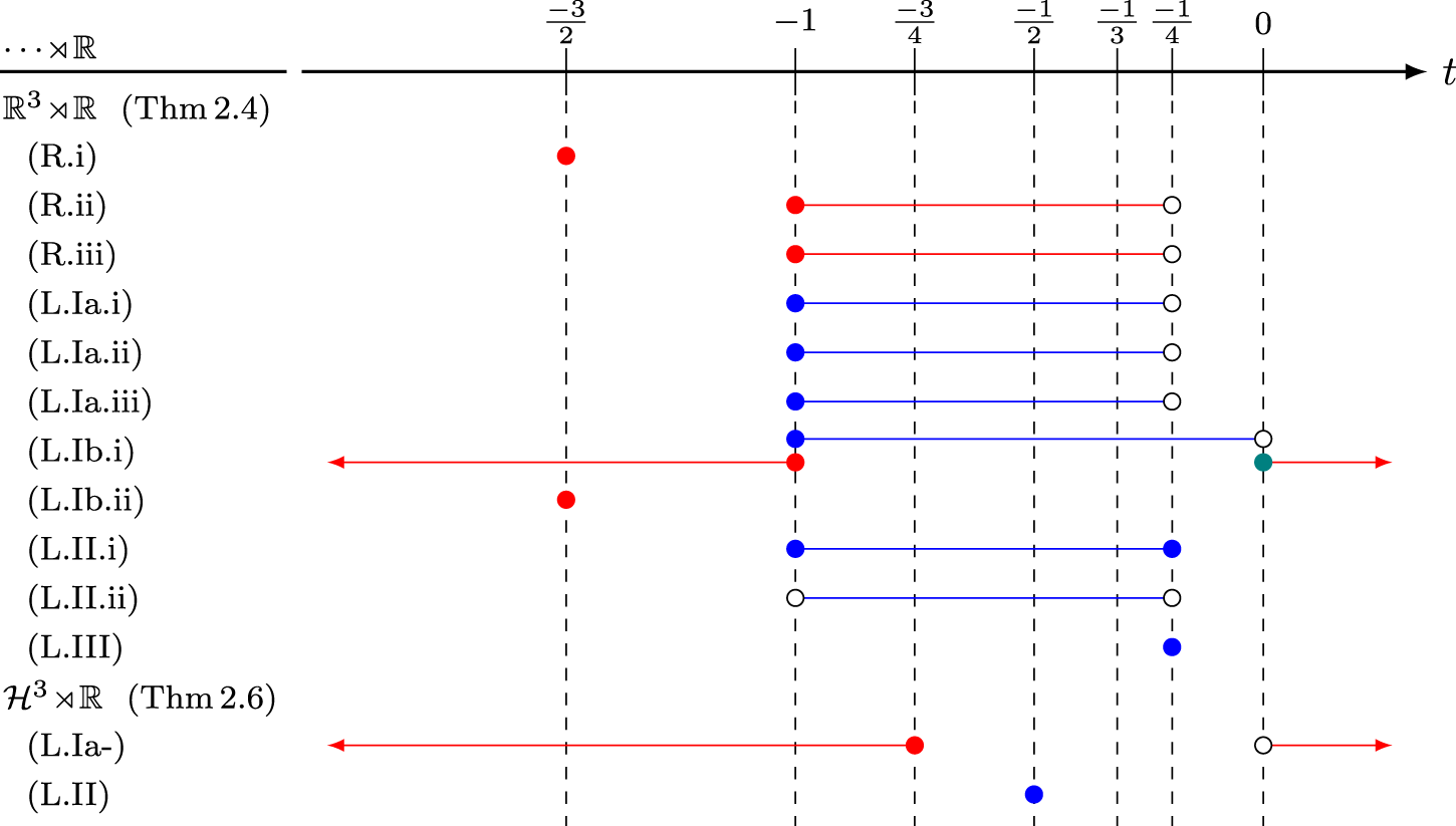


 Open access