Hydraulic potential

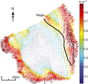
A basal hydraulic potential gradient map (Fig. 2) was generated from the surface and basal elevation maps of Reference Sanders, Cuffey, MacGregor, Kavanaugh and DowSanders and others (2010). Following Reference ShreveShreve (1972), hydraulic potential gradients were calculated assuming that basal water pressures are everywhere equal to the ice overburden pressure. While the true gradients will differ due to variations in basal conditions, this first-order approximation allowed identification of areas through which basal waters might be routed. At overburden pressure, the largest gradients are observed near the glacier’s margins. The direction of the gradient vectors suggests that water originating near the headwall flows both into the overdeepening and along the side margins.

Fig. 2. Hydraulic potential gradient map calculated for WWG. Basal water pressures are assumed to be at overburden. The vector color scale shows meters of hydraulic potential change per meter. The arrowheads show the direction of the hydraulic potential gradient. The approximate location of the riegel is indicated by the black curve.

Borehole camera surveys

We classify englacial features into two morphological categories: fractures (generally planar features assumed to result primarily from ice stress conditions) and channels (features with roughly circular cross sections, assumed to form through water flow, although potentially initiated within fractures). In the nine primary boreholes, 22 identifiable channels and eight fractures were observed. In the discussion that follows, channels located in the top 25m are referred to as ‘shallow englacial channels’; channels at greater depths are referred to as ‘deep englacial channels’. A differentiating depth of 25m has been chosen based on the argument that surface crevasses do not penetrate below this depth (Reference Cuffey and PatersonCuffey and Paterson, 2010). In total, 18 shallow englacial channels were identified in the nine boreholes, most of which were above the borehole water level at the time of survey (Fig. 3). Of the shallow channels, 13 had water flowing through them, detected when the channel was above the borehole water level; below the borehole water level no flow was visible through any of the englacial features (including deep englacial channels and fractures). In total, four deep englacial channels were observed (Fig. 3), described in Table 2. In addition, eight open englacial fractures were intersected, the largest of which was ∼12 cm wide, and they appear to be similar in form to those discussed by Reference PohjolaPohjola (1994), Reference Fountain, Jacobel, Schlichting and JanssonFountain and others (2005) and Reference Harper, Bradford, Humphrey and MeierbachtolHarper and others (2010). Characteristics of these fractures are described in Table 3.

Fig. 3. Results from video camera logs of the nine surveyed boreholes at WWG. The boreholes in bold are those that were instrumented. Boreholes are clustered firstly with respect to their location on the ice surface and secondly with respect to borehole depth

Instrument records

Ten sensors were installed in four boreholes, comprising four pressure transducers, three temperature sensors and three conductivity sensors. Records for all instruments exhibited variations on a range of timescales; here we focus primarily on diurnal signals in the records due to their well-documented relationship to variations in surface meltwater production (Reference Iken and BindschadlerIken and Bindschadler, 1986; Reference Flowers and ClarkeFlowers and Clarke, 2002; Reference Schuler, Fischer and GudmundssonSchuler and others, 2004; Reference Fudge, Humphrey, Harper and PfefferFudge and others, 2008). In this study, water-pressure values are presented in units of pressure head (m).

A Campbell Scientific CR10X data logger was used to calibrate the pressure transducers (in borehole H1). Following installation, however, the transducers were monitored using a Campbell Scientific CR1000 data logger. The default measurement integration times employed by these two data loggers differ: 2.72 ms and 250μs, respectively. The shorter integration time of the CR1000, coupled with the long (∼250 m) wire lengths used at the glacier, resulted in small, capacitance-induced errors in measured voltages. These errors, which were first recognized as small voltage changes at times when additional sensors were connected to the data logger, were corrected by applying a constant scaling factor to the voltage (determined by the size of the observed voltage change). These capacitive effects result in systematic fractional errors with magnitudes <2m for P4, <1m for P6 and <3m for P8.

Because borehole H10 was blocked by a rock at a height well above the bed, inclinometry measurements could not be made. It is therefore not possible to determine the true height of sensor P10 (which was installed just above the obstructing rock) above the bed. While a ground-penetrating radar (GPR) survey by Reference Sanders, Cuffey, MacGregor, Kavanaugh and DowSanders and others (2010) suggests an ice thickness of 160 ± 10m in the location of borehole H10, comparison of early transducer output values (prior to the borehole freezing) with ice overburden calculations suggests that the ice thickness is at the lower end of this range. The pressure values shown in Figures 4e, 5c and d and 9 were therefore calculated assuming an ice thickness of 150m. Because of the systematic uncertainty in ice thickness (approximately equal to that of the GPR survey, or ∼20m), no flotation pressure has been calculated for the P10 record. It is worth stressing that any such error would result in a systematic shift of the whole P10 record without changing the waveform; the 2σ random error of individual P10 measurements (calculated from the calibration data) is constant at ±0.06 m.

Fig. 4 Pressure records for the instrumented boreholes from 18 August (day 230) to 16 December (day 350) 2007.(a) Hourly average air temperatures from AWS 1;0°C is shown by the dashed line. (b–e) P4 (b), P6 (c), P8 (d) and P10 (e) records; the dashed lines respresent our best estimate of the local flotation pressure in H4, H6 and H8.

Fig. 5. Pressure and water temperature values recorded between 17 September (day 260) and 6 November (day 310) 2007. (a) Hourly average air temperatures from AWS 1; 0°C is shown by the dashed line. (b) Basal water temperatures recorded by T4 (plotted in black, relative to the supercooling minimum) compared with P4 pressure (green). (c) Comparison between P8 (black) and P10 (blue) pressures. (d) Relative pressure change recorded by P4 (green), P8 (black) and the inverse of the P10 record (blue). The shaded regions delineate the two 5 day time periods, i and ii, referenced in Figure 9.

Figure 4 shows borehole pressure records for boreholes H4, H6, H8 and H10, compared with air temperature records from AWS1 for the period 18 August (day 230) to 16 December (day 350) 2007. Figure 5 shows the records for boreholes H4, H8 and H10 at a higher temporal resolution, between 17 September and 6 November (days 260–310) 2007. Pressures recorded by P4 varied up to ∼27m on a diurnal timescale (Fig. 4b; day 234). P6 water pressure varied diurnally by ∼4m during the summer melt season. P8 water pressure varied diurnally by 3–8m during summer 2007 (Fig. 5c). Rises in P4, P6 and P8 pressure generally coincided with warming surface air temperature during summer 2007 (as can be seen during several intervals in Fig. 6a and b), with lags of <2 hours. Variations in P10 pressure (Fig. 5c) were anti-phased with respect to changes in P4 and P8 pressure.

Fig. 6. Borehole pressure and conductivity records between 5 September (day 248) and 13 September (day 256) 2007. (a) Hourly average air temperatures from AWS 1; 0°C is shown by the dashed line. (b) C4 conductivity (black solid curve) and P4 pressure (blue dashed curve). The black dashed line shows our best estimate of the flotation pressure. (c) C6 conductivity (black solid curve) and P6 pressure (blue dashed curve). (d) C8 conductivity (black solid curve) and P8 pressure (blue dashed curve) with our best estimate of the flotation pressure indicated by the black dashed line

Thermistors were calibrated prior to installation by submerging them in water-saturated snow on the glacier surface. Unfortunately, the resulting voltage values were too inconsistent (likely due to solar heating of the instruments in the shallow surface snow) to provide a satisfactory calibration. In addition, the long wire lengths used introduced capacitance errors similar to those observed in the pressure records. Because of these errors, accurate determination of the 0°C point in each of the temperature records is difficult. (As in the case of the pressure records, zero-point errors are systematic, and affect the record uniformly.) Both random measurement and thermal drift errors of the thermistors are very low, at ∼0.01°C and ∼0.001 °Ca⁻¹, respectively (Reference Zurbuchen and DaytonZurbuchen, 2000); as a result, magnitudes of variations in basal water temperature are well constrained. In order to obtain the most conservative (i.e. coolest reasonable) estimate of basal water temperatures, we here assume that the greatest resistance value indicated in each thermistor record corresponds with the pressure-melting point (pmp) of the maximum ice thickness (∼185 m) measured during the GPR survey of Reference Sanders, Cuffey, MacGregor, Kavanaugh and DowSanders and others (2010). This corresponds to a pmp of −0.16°C, which we refer to as the ‘supercooling minimum’, and includes a compensation of −0.04°C for impurities in the basal water (Reference HarrisonHarrison, 1975). The supercooling minimum assumption allows for the possibility that the minimum observed values result from upwelling of water from the deepest portion of the cirque bowl. Thermistor record noise was removed with a Butterworth low-pass filter with cutoff frequencies of 2 hours (T4) or 6 hours (T6 and T8), determined by the level of noise in the individual records.

Figure 7 shows basal water temperature records for H4, H6 and H8 between 18 August and 16 December (days 230–350) 2007; as H10 was blocked some distance above the bed, no temperature measurements were made in this borehole. In general, temperatures in borehole H4 (Fig. 5b) varied inversely with respect to water-pressure changes observed in the borehole (cf. Fig. 8a and b), and exhibited variations on diurnal timescales as large as 0.8°C (day 255). The T6 temperature record (Fig. 7b) also exhibits variations on diurnal timescales (up to 0.58°C; day 255) that are anti-phased with respect to changes in P6 pressure (cf. Fig. 8a and b). In contrast, T8 water temperature fluctuated over a smaller (0.05°C) range, with little discernible correspondence between T8 temperature and P8 pressure, although one event with anti-phased correspondence occurred on 22 October (day 295; not shown). Comparison between temperatures recorded in boreholes H4 and H6 (Fig. 8a; dashed and solid lines, respectively) for the period 18 August (day 230) to 2 September (day 245) 2007 shows that diurnal temperature variations were similar in form in the two boreholes, with variations recorded by T6 exhibiting smaller amplitudes than those recorded by T4. Because these temperature data were recorded by two separate data loggers (sampling sensors in two separate boreholes), these variations are unlikely to be measurement artifacts.

Fig. 7. Basal water temperature records from 18 August (day 230) to 16 December (day 350) 2007 recorded by (a) T4, (b) T6 and (c) T8 with the lowest temperatures referenced to the supercooling minimum (determined for the maximum ice thickness). The dashed line shows 0°C.

Fig. 8. Basal water temperature and pressure records from 18 August (day 230) to 2 September (day 245) 2007. (a) T4 (black solid curve) and T6 (red dashed curve) water temperatures with the lowest temperature corresponding to the supercooling minimum (determined for the maximum ice thickness). The black dashed line shows 0°C. (b) P4 (black solid curve) and P6 (blue dashed curve) pressure records.

Conductivity sensors were calibrated prior to installation against an HI 8733 Multi-Range Conductivity Meter (accuracy ±1% at 20°C). The random errors produced using this method were calculated using linear regression with two standard deviations: C4 (±0.09μS cm⁻¹), C6 (±0.16μS cm⁻¹) and C8 (±0.08μS cm⁻¹). Noise on the electrical conductivity time series has been removed with a Butterworth low-pass filter with a cut-off frequency of 1 hour.

Figure 6b (black solid curve) shows records from conductivity sensor C4, which recorded diurnal variations over a small range of several μScm⁻¹; these fluctuations were generally inverse with P4 pressure change (Fig. 6b, blue dashed curve). Similarly, the C6 conductivity record indicates a negative relationship with variations in P6 pressure (Fig. 6c, solid and dashed curves, respectively); conductivity values in borehole H6 varied by <1μScm⁻¹ on diurnal timescales. Although there was only minimal correspondence between the C8 conductivity record and changes in P8 pressure, several brief events indicated an inverse relationship (Fig. 6d, solid and dashed curves, respectively).

Drainage system

Several studies have suggested that drainage in overdeepened regions is dominated by englacial transport. For example, Hooke and others have argued that if the adverse slope of a riegel is sufficiently steep, subglacial water will be forced into an englacial system, thus bypassing the overdeepening (Reference Hooke, Miller and KohlerHooke and others, 1988; Reference HookeHooke, 1991; Reference Hooke and PohjolaHooke and Pohjola, 1994). Reference Fountain and WalderFountain and Walder (1998) have additionally suggested that, over time, englacial channels migrate downward through the ice, becoming pinned at the elevation of a riegel lip and resulting in near-horizontal transport through the ice. At WWG the majority of observed englacial drainage features were conduits at shallow (<25 m) depth associated with open surface fractures or with paleo-fractures that had closed through ice deformation, and are therefore too shallow to represent the overdeepening englacial channels discussed by either Reference Hooke and PohjolaHooke and Pohjola (1994) or Reference Fountain and WalderFountain and Walder (1998). None of the observed deep channels at WWG trended down-glacier, which would be expected if they formed an active englacial drainage network. In addition, most of the fractures observed at greater depths dipped steeply towards the glacier bed in the down-glacier direction and are therefore unlikely to facilitate englacial flow over the riegel lip. Several of the boreholes were blocked at some point along their length by rocks, which prevented video surveys of their lower portions; in other boreholes, visibility was restricted by high post-drilling turbidity levels. The total length of borehole above the level of the riegel (i.e. where channels would need to be located in order to transport water over the riegel lip in the manner of Reference Hooke and PohjolaHooke and Pohjola (1994) and Reference Fountain and WalderFountain and Walder (1998)) that could not be surveyed with the borehole camera was small, accounting for just ∼10m in H4, ∼14m in H5, ∼15m in H6, ∼2m in H7 and ∼35m in H10 (Fig. 3). However, the small number of boreholes drilled means that only a minor fraction of the ice in the study region was sampled. Thus, while no compelling evidence for englacial water transport was observed, it is possible that significant englacial flow features were missed. Further studies (including the drilling and video survey of additional boreholes) will be necessary to determine whether englacial water transport is significant at WWG.

Given that all the boreholes intersected englacial features, it is important to determine whether the observed instrument variations resulted from supraglacial, englacial or basal forcings. Substantial water-pressure variations were observed in all instrumented boreholes. However, field observations at WWG indicate that the near-surface portions of the boreholes typically freeze closed within 1 week (as was observed during summer 2006). Thus, ‘pollution’ of the water-pressure signal from supraglacial sources and shallow englacial features is likely limited to the beginning of the instrument records. Additionally, there was no evidence for water flow through deep englacial channels or fractures in any of the boreholes during the video survey. It should be noted, however, that boreholes H8 and H9 exhibited drops in water level during drilling at depths that correspond with fractures observed in the video surveys (Table 3). Given the lack of visible water flow through these fractures, it is not possible to determine whether they were connected to an englacial drainage system.

During the summer of 2007, the pressure records of P4, P6 and P8, for the most part, varied positively with respect to changes in surface air temperature, with lags of <2 hours. During this time, basal water-pressure values typically ranged within ∼65–105% of overburden. Similar pressure variations have been interpreted as indicators of flow through a distributed subglacial hydrological system in several studies (e.g. Reference Harper, Humphrey, Pfeffer, Fudge and O’NeelHarper and others, 2005; Reference Lappegard and KohlerLappegard and Kohler, 2005). Given the small number of boreholes drilled at WWG, it is possible that a subglacial channelized system operated alongside a distributed system; however, none was observed. Water-pressure variations continued until day 337, by which time air temperatures had remained continuously below freezing for ∼40 days (Fig. 4). It is unlikely that these late-season water-pressure variations resulted from the input of surface water; this suggests a basal origin for the variations. The instrument and borehole observations recorded at WWG therefore provide compelling evidence for the presence of an active basal drainage system near the northern margin of the glacier.

Several observations indicate that substantial areas of the glacier are underlain by soft sediments. Highly turbid water was observed at the base of all boreholes thought to reach the bed. This was likely due to disturbance of unconsolidated basal materials by the hot-water drill. Alternately, the observed high-turbidity waters could have resulted from the melting of sediment-rich basal ice: debris-rich layers ∼30–50 cm thick were observed in ice-marginal caves, and borehole video showed a ∼30 cm thick unfrozen wedge of sediment at the bottom of borehole H8; these observations also suggest the presence of basal sediments. Furthermore, when borehole H5 was re-drilled in summer 2008 for repeated borehole inclinometry (Reference Sanders, Cuffey, MacGregor, Kavanaugh and DowSanders and others, 2010), the wire weight (which upon installation in summer 2007 was suspended 30 cm above the ice/bed interface) was sediment-covered upon retrieval. This suggests that basal materials intruded some distance into borehole H5. When coupled with the evidence for a distributed basal drainage system discussed above, these observations indicate that basal water flow at WWG in the study region was likely to have been primarily within a subglacial aquifer (e.g. Reference Stone and ClarkeStone and Clarke, 1993; Reference Fountain and WalderFountain and Walder, 1998; Reference Jansson, Hock and SchneiderJansson and others, 2003).

Basal water temperature

Both field-based and modeling studies of glacier hydrology generally assume that water flowing englacially or at the ice/bed interface is thermally equilibrated with the surrounding ice (e.g. Reference LliboutryLliboutry, 1971; Reference RöthlisbergerRöthlisberger, 1972; Reference ShreveShreve, 1972; Reference Iken and BindschadlerIken and Bindschadler, 1986; Reference ClarkeClarke, 1987; Reference Flowers and ClarkeFlowers and Clarke, 2002; Reference Bates, Siegert, Lee, Hubbard and NienowBates and others, 2003). It is postulated that subsurface waters flow at the pmp, and that any excess heat gained from flow or geothermal sources is used to warm or melt the ice adjacent to the channel (Reference Alley, Lawson, Evenson and LarsonAlley and others, 2003a; Reference ClarkeClarke, 2005; Reference Tweed, Roberts and RussellTweed and others, 2005). The temperature records plotted in Figures 5b, 7 and 8a show significant diurnal variations above the pmp and indicate that this assumption of thermal equilibration of subglacial water is not always valid.

Diurnal variations recorded by T4 were generally anti-phased with respect to water-pressure changes recorded by P4 (see Figs 5b and 8); variations in the records of T6 and P6 are similarly anti-phased. These records argue for a basal source for the temperature variations, as water flowing englacially would thermally equilibrate to the surrounding ice in the period between water input at the surface and transport to the thermistors installed at the base of the boreholes and, as a result, would not retain any diurnal water temperature signals. Furthermore, if any heat was advected by warm surface waters or generated by viscous flow, it would be greatest at times of peak water input, so any temperature and pressure variations resulting from englacial flow would be expected to be in-phase or nearly so.

Reference ZotikovZotikov (1986) argued that geothermal energy is the primary source of heat for warming subglacial water; water could also be warmed on the headwall prior to flowing into the glacier basal system. As WWG moves slowly (<10ma⁻¹; Reference Sanders, Cuffey, MacGregor, Kavanaugh and DowSanders and others, 2010), any warming by basal friction and strain heating is likely to be negligible. The observed temperature signals might be explained by the vertical movement of water into and out of the subglacial sediment aquifer at WWG. At times of high meltwater input (and hence high drainage system pressure), glacially cooled water could be forced downward into the sediment, lowering temperatures at the ice/bed interface. At times of low basal pressure, relatively warm groundwater could move upward towards the glacier sole (driven by the higher water table in the steep flanks of the armchair-like headwall at WWG). This interpretation is supported by the electrical conductivity measurements. Changes in conductivity in boreholes H4 and H6 were largely inversed with respect to changes in basal water pressure (Fig. 6b and c), with decreased conductivity values at times of high pressure (i.e. when water is forced downward into the sediments) and increased conductivity values at times of low water pressure (when pore-water is drawn out of the sediments). Alternatively, low conductivity values concurrent with high basal water pressure might reflect fresh surface water input into the basal system (Reference CollinsCollins, 1979). In either case, conductivity values likely indicate the length of time the water has been in contact with basal materials (Reference CollinsCollins, 1979; Reference Gurnell and FennGurnell and Fenn, 1985). The observed variations in conductivity are unlikely to result from englacial flow given the low sediment content of the bulk of the glacier ice. Groundwater flow has been previously reported to raise subglacial water above the local pmp by Reference BayleyBayley (2007), and modeling studies by Reference Flowers and ClarkeFlowers and Clarke (2002) and Reference Kavanaugh and ClarkeKavanaugh and Clarke (2006) have suggested that diurnal variations in water pressure at the ice/bed interface can drive a vertical flux of water into and out of a basal sediment aquifer.

As noted above, capacitance effects prevent the 0°C point in the borehole temperature records from being known. The assumption that the lowest value recorded in each thermistor record corresponds to a temperature of −0.16°C (the supercooling minimum, i.e. the pmp of 185m thick ice including a correction of −0.04°C for the potential presence of solutes in the water) results in relatively warm overwinter temperatures (averaging ∼0.31°C in H4, ∼0.39°C in H6 and ∼0.09°C in H8) and a maximum indicated basal water temperature of ∼0.75°C in H4 (i.e. ∼0.91°C above the supercooling minimum). If the minimum temperature value in each record is assumed to correspond to the local pmp, overwinter temperatures and temperature peaks in summer 2007 are warmer still. Conversely, if we assume that the stable winter values represent local pmp values, the resulting minimum temperature values are unreasonably low (at −0.43 to −0.13°C) and, given that the electrical conductivity values recorded beneath the glacier appear too low to significantly suppress the pmp, water would likely freeze at these temperatures. This suggests that stable overwinter temperatures are higher than the local pmp. Insight into the probable range of subglacial water temperatures at WWG might be gained by comparison with temperatures recorded beneath Trapridge Glacier, Yukon, Canada, a glacier also underlain by sediment. During July 1998 at Trapridge Glacier, Analog Devices AD590 temperature sensors were installed to depths of 0.15–0.19m in the basal sediments. Temperatures up to 1.1°C and diurnal swings as large as ∼0.4°C were recorded, with temperatures rising above the pmp. The WWG and Trapridge Glacier water temperature records suggest that (1) temperature variations of ∼0.4–0.8°C occur on diurnal (and other) timescales beneath both glaciers and (2) at times, basal water temperatures at both WWG and Trapridge Glacier exceed the local pmp.

If accurate, the relatively high overwinter temperatures shown in Figure 7 might help explain the late-season water-pressure variations at WWG. The records of sensors P4, P8 and P10 exhibit pressure variations until 3 December (day 337) 2007. This shutdown is late in comparison with other glacier systems. For example, at Bench Glacier, Alaska, stable winter-mode conditions have been observed to set in around the end of September (Reference Fudge, Humphrey, Harper and PfefferFudge and others, 2008), and basal pressure variations at Trapridge Glacier have been seen to cease in mid-September (Reference FlowersFlowers, 2000). At WWG, pressure variations persisted long after air temperatures dropped below freezing (Fig. 4), suggesting that water continued to flow through the subglacial system after cessation of surface melt. One possibility is that warm waters might have slowly upwelled from a subglacial aquifer throughout the winter months. The persistence of above-freezing water temperatures might also have been aided by the movement of sediments up into the boreholes (as was observed in H5); this sediment could have provided the basal thermistors with a measure of insulation from the surrounding ice.

Both the above-freezing values and the time-varying nature of these basal water temperature records suggest that the assumption that subglacial waters are everywhere at the pmp oversimplifies reality, and indicates that additional investigation is needed if the conditions that control basal melt and freeze-on (such as flow up adverse basal slopes; e.g. Reference Alley, Lawson, Evenson, Strasser and LarsonAlley and others, 1998, Reference Alley, Lawson, Evenson and Larson2003a; Reference Tweed, Roberts and RussellTweed and others, 2005) are to be understood.

Hydraulic jacking

Examination of the borehole water-pressure records of Figure 5 shows that pressure variations recorded by P10 during days ∼260–310 are nearly perfectly inverted with respect to those in the records of P4 and P8 (see Fig. 5c and d, with the latter showing relative pressure changes in these three boreholes with P10, in blue, plotted as an inverse record). These records are so strongly anticorrelated that it is reasonable to suspect that the inverted response of P10 is the result of an error in wiring or logging of one or more of the sensors. However, while sensors P4 and P8 were logged by one CR1000 data logger, P10 was logged by another; the same program was used in both loggers. Identical calibration procedures were used with all pressure transducers, and the variation of signal voltage with pressure (i.e. depth in water) was very similar for all transducers. All transducers recorded the correct values for the depth of installation on the day of borehole instrumentation, and the record for P10 was not inverted with respect to those of P4 and P8 prior to day 260. These factors indicate that the records of P4, P8 and P10 accurately represent real pressure variations.

To further investigate the observed pressure relationships, we performed cross-correlation analysis of records for P4, P8 and P10 during two 5 day intervals (indicated by shaded regions in Fig. 5c and d). The first interval, labeled i, spans 2–7 October (days 270–275); the second, labeled ii, spans 27 October–1 November (days 300–305). Pearson product-moment correlation coefficients are shown in Table 4; correlations were performed on both unmodified and linearly detrended records. Correlations between P4 and P8 are strongly positive (r ² ≥ +0.85) with zero lag, while negative correlations between P10 and both P4 and P8 are strongly negative (r ² ≥ −0.77) with lags of 14– 32min. In comparison, correlations between air-temperature and water-pressure values are weaker (r ² ≤ 0.46) with lags of ∼7–21 hours. (While pressure values were recorded every 2 min, air temperatures were recorded as hourly averages; this results in a lower time resolution for lags between pressure and air-temperature values.) These correlations suggest that air temperatures had only weak influence on basal water pressure during these time periods; this interpretation is supported by the fact that recorded air temperatures were <0°C (suggesting low surface meltwater production rates) during much of interval i and all of interval ii.

The relationships between the records of P4, P8 and P10 are further explored in the phase diagrams of Figure 9. In these diagrams, P10 pressure values are plotted against P4 (Fig. 9a and c) and P8 (Fig. 9b and d) values during the two time intervals. These diagrams show nearly linear, but inverted (i.e. trending from upper left to lower right) relationships between P10 and both P4 and P8. The near-linearity of the relationships seen in Figure 9 indicates that a given pressure change in the hydraulically connected region (as recorded by P4 and P8) induced a response in the area of the bed sampled by P10 that was invariant with drainage system pressure. The clockwise hysteresis visible in the phase diagrams indicates that pressure changes in boreholes H4 and H8 occur slightly before the corresponding changes in H10. Similar anti-phased variations in pressure between boreholes were reported at Trapridge Glacier by Reference Murray and ClarkeMurray and Clarke (1995); in that study, however, the magnitude of the response in the unconnected region was strongly dependent upon water pressure in the connected region of the bed. Murray and Clarke argued that water pressure variations in hydraulically connected regions of the bed can result in changes in the distribution of ice overburden stresses between connected and unconnected regions of the bed. Our records suggest that a similar mechanism operated at WWG during portions of the study interval. The instrument records discussed in the Results section indicate that the bed in the near-marginal region of the glacier was hydraulically connected to a sediment-based, distributed subglacial drainage system. In contrast, the region of the bed sampled by H10 appears to have been hydraulically isolated, at least on timescales relevant to the observed pressure variations. (As noted above, much of the study region appeared to be underlain by sediments, through which water would be expected to flow. The near-perfect anticorrelation between the pressure records seen in Figure 9 suggests that any such flow is slow enough in the region of H10 to be masked by the more rapidly varying changes in overburden stress driven by drainage system pressure in the near-margin connected region. The strong anticorrelation between pressure records was not seen prior to day ∼260; this suggests that some water flow was present in the region of H10 earlier in the melt season.) As water enters the near-marginal drainage system, the glacier ice is forced upwards; because ice is rigid on short timescales (Reference Cuffey and PatersonCuffey and Paterson, 2010) this uplift is translated towards the center of the overdeepening. This results in a decrease in the vertical normal stress acting at H10 and a reduction in water pressure. When the input of meltwater to the hydraulically connected region decreases, the ice settles back down; this reloads the bed at H10 and results in an increase in water pressure there. This ‘hydraulic jacking’ mechanism provides the most plausible explanation for the pressure records of P4, P8 and P10. Although the peak jacking force would be expected at the time of peak water pressures in the subglacial drainage system, the small (∼14–32 min) lag observed in the response of P10 with respect to variations in P4 and P8 pressures might suggest that the jacking signal reflects changes in subglacial water volume, rather than pressure. If this is the case, the greatest transfer of ice-overburden pressure between regions of the bed (and hence minimum pressures at H10) would correspond to maximum vertical uplift of the ice. The lag in the record of P10 might therefore represent the difference in time between peak pressure and peak water volume in the subglacial drainage system.

Fig. 9. Phase plots of pressure records from days 270–275 (interval i in Fig. 5) and days 300–305 (interval ii in Fig. 5). (a) P4 against P10 from days 270–275. (b) P8 against P10 from days 270–275. (c) P4 against P10 from days 300–305. (d) P8 against P10 from days 300–305.

The apparent near-perfect short-term hydraulic isolation of H10 allows estimation of the amount of uplift necessary to generate the observed hydraulic jacking signal. Let us consider a body of water contained within a rigid basin (which is thus confined laterally so any changes in water volume results solely from vertical expansion or compression) and initially pressurized to some value, P ₀, by a force acting uniformly on a rigid lid. Following Reference ClarkeClarke (1987), we assume that the water density, ρ _w, is related to the pressure, P, acting upon it by

where β = 5.10 × 10⁻¹⁰ Pa⁻¹ is the coefficient of compressibility for water. If we decrease the pressure acting upon the parcel by 100 kPa (1 bar, or ∼10m of pressure head), the fractional density change is ρ _w(P)/ρ _w(P ₀) = 0.99995; this corresponds to a volumetric increase of 0.005%. If the confining vessel is rigid, a pressure decrease of 100 kPa acting upon a body of water with an initial uniform thickness of 1.0 m will result in a vertical expansion of 0.05mm by the water; conversely, if the lid is, instead, displaced upwards by 0.05mm, the pressure within the body of water will decrease by 100 kPa. If (1) the glacier ice acts as a rigid body over the relevant timescales, (2) vertical displacements in the ‘active’ jacking region (i.e. in the hydrologically connected region of the bed) translate uniformly to the ‘passive’ (or hydrologically isolated region of the bed) and (3) the body of water sampled by sensor P10 is well isolated (as is suggested by the high r ² values shown in Table 4), the amount of jacking required to generate pressure-head changes of magnitudes similar to those observed in the record of P10 might be vanishingly small. (In fact, if the effective thickness of the water body sampled by P10 is similar to, or less than, the 1.0m thickness assumed here, it is possible that the observed signals could result from water-pressure driven dilatant expansion of sediments in the near-marginal basal drainage system, rather than by direct lifting by the water (Reference ClarkeClarke, 1987; Reference Kavanaugh and ClarkeKavanaugh and Clarke, 2006).) Because the amount of vertical displacement required to generate the observed jacking signal is small, it is possible that only a small volume of water is needed to drive it. For example, only 3.0m³ of water would be needed to lift a hydraulically ‘active’ region with dimensions of 200m × 300m upward by 0.05 m, and only 50m³ of water would be needed to uniformly lift the entire ∼1km² glacier by a similar amount.

Implications of observations for water flow and cirque erosion

The characteristics of the hydrological system operating at WWG (particularly with respect to sediment transport capacity; e.g. Reference Alley, Cuffey, Evenson, Strasser, Lawson and LarsonAlley and others, 1997, Reference Alley, Lawson, Larson, Evenson and Baker2003b; Reference Riihimaki, MacGregor, Anderson, Anderson and LosoRiihimaki and others, 2005) will strongly influence erosional patterns within the glacial cirque (e.g. Reference HookeHooke, 1991; Reference Alley, Lawson, Larson, Evenson and BakerAlley and others, 2003b). Waters in the northern near-marginal portion of the study area appear to move through a distributed, sediment-based basal drainage network. Removal of sediment through such a system is likely less efficient than it would be, for example, in a fast-flowing, channelized drainage system (Reference Alley, Lawson, Evenson and LarsonAlley and others, 2003a; Reference Riihimaki, MacGregor, Anderson, Anderson and LosoRiihimaki and others, 2005). This, plus the general slowing of flow argued to occur as subglacial water moves up over a riegel (e.g. Reference Alley, Lawson, Larson, Evenson and BakerAlley and others, 2003b), suggests that sediments are a persistent feature in the study area.

Variations in subglacial water pressure are thought to significantly increase quarrying of underlying materials through the redistribution of basal stresses (e.g. Reference IversonIverson, 1991; Reference Cohen, Hooyer, Iverson, Thomason and JacksonCohen and others, 2006). It is generally assumed that the presence of subglacial sediments limits basal erosion by reducing joint breakage, plucking and abrasion (e.g. Reference HookeHooke, 1991; Reference Alley, Cuffey, Evenson, Strasser, Lawson and LarsonAlley and others, 1997). Reference HookeHooke (1991) further argued that the deposition of sediments on adverse bed slopes can provide an important control on the erosion (and hence form and evolution) of overdeepened basins. However, the hydraulic jacking indicated by the records of P4, P8 and P10 might significantly impact basal erosion rates at WWG through repeated loading and unloading of the glacier bed and a near-continuous redistribution of basal stresses between pinning points in a manner similar to that argued by Reference IversonIverson (1991) and Reference Cohen, Hooyer, Iverson, Thomason and JacksonCohen and others (2006). Furthermore, Reference Kavanaugh, Moore, Dow and SandersKavanaugh and others (2010) reported extensive water-pressure pulse activity (generated by abrupt basal motion; Reference KavanaughKavanaugh, 2009) at WWG between August 2008 and May 2009. Pressure pulse activity at WWG during this interval was significantly higher than observed at either of the two other glaciers where pressure pulse studies had been conducted, Trapridge Glacier and Storglaciären, Sweden (Reference KavanaughKavanaugh, 2009; Reference Kavanaugh, Moore, Dow and SandersKavanaugh and others, 2010). The elevated pulse activity at WWG might result from hydraulic jacking-induced redistribution of basal stresses, and might further indicate that the overdeepening is still actively eroding by transmitting pressure through the sediment layer to the bedrock (Reference Kavanaugh, Moore, Dow and SandersKavanaugh and others, 2010). Further research will be necessary to clarify both the role that basal sediments play in modifying erosional patterns beneath cirque glaciers and the significance of hydraulic jacking for cirque erosion.

The hydraulic potential map shown in Figure 2 implies that subglacial flow crosses the overdeepening. In contrast, the hydraulic jacking signal discussed above indicates that the glacier bed in the vicinity of borehole H10 is hydraulically isolated, which suggests that the hydraulic potential map provides a poor approximation for the subglacial flow paths in this region of the bed. The potential map was constructed by assuming that basal water pressure everywhere equals the overburden. It is likely, instead, that basal water pressures adjust to differences in inputs and drainage. Note, in particular, that the hypothesized potential gradients from the headwall into the overdeepening dramatically weaken and continue to be weak throughout the overdeepening. The transition from strong to weak gradients suggests that water would build up at the upstream edge of the overdeepening, increasing pressures and hydraulic potential. Such an increase, in turn, could either (1) divert water toward the margin of the glacier or (2) allow the opening of subglacial cavities or a change in sediment porosity that would facilitate flow through the overdeepening. Our borehole studies suggest the former, with basal waters at WWG avoiding the overdeepening by flowing near the glacier margin in a manner similar to flow configurations observed in some overdeepened regions of valley glaciers (Reference Hantz and LliboutryHantz and Lliboutry, 1983; Reference LliboutryLliboutry, 1983; Reference FountainFountain, 1994). It is possible that the presence of low-permeability sediments limits, or prohibits, flow towards the center of the overdeepening. Were water able to more freely move towards the glacier center, pressure variations in borehole H10 would likely appear as delayed and dampened (rather than inverted) versions of the variations observed in H4 and H8. These observations suggest that flow paths derived solely from hydraulic potentials should be viewed with some skepticism, and that spatial variations in hydraulic conductivity can have a strong effect on the movement of subglacial water.