2. Ambient seismic excitation at the WAIS Divide site

2.1. Ambient noise interferometry

The broad use of ambient noise methods over the past few decades has sparked a revolution in imaging and temporal monitoring in seismic settings at a multitude of scales. In short, works by Snieder (Reference Snieder2004), Wapenaar and Fokkema (Reference Wapenaar and Fokkema2006), Wapenaar and others (Reference Wapenaar, Draganov, Snieder, Campman and Verdel2010) and Campillo and Paul (Reference Campillo and Paul2003) demonstrated that under certain conditions, the cross-correlation of multiply scattered or otherwise isotropically excited wavefields at two receivers results in an approximation of the impulse response function between those two receivers. Given that at lower frequencies the seismic wavefield is either isotropically excited or at least predictably excited by the presence of a coastline, this relationship has been broadly exploited to reconstruct surface waves (Ritzwoller and others, Reference Ritzwoller, Lin and Shen2011) and body waves (Nakata and others, Reference Nakata, Chang, Lawrence and Boue2015) for a number of imaging applications. If the wavefield is isotropic then the following holds:

(1)$$\eqalign{\left\langle u( x_A,\; t)\, \ast\, u( x_B,\; -t) \right\rangle = [ G( x_A,\; x_B,\; t) + G( x_B,\; x_A,\; -t) ]\, \ast \,S( t) }$$

Here, u(x _A,B,  t) denotes the wavefield recorded at receiver A or B, the * denotes a convolution, with the time reversal turning it into a correlation, and G(x _A,  x _B,  t) represents the Green's function between receivers A and B. S(t) is the autocorrelation of the noise and essentially represents the wavelet convolved into the Green's function. A given wavepath in the Green's function is correctly reconstructed if there are sources distributed along its stationary zone (Snieder, Reference Snieder2004). For instance, a correctly reconstructed Rayleigh wave between two surface receivers requires surface sources distribute along the end points of the station pair line. We rebuilt Rayleigh waves through anthropogenic noise in the following study, and as such, we generally limited our study to interstation paths that aligned with a known anthropogenic noise source, WAIS Divide camp.

2.2. Noise correlations on the TIME array

As a first step to identify the nature of seismic waves supported by the firn and underlying glacial ice, we performed daily average cross-correlations of ambient noise between all interstation component pairs. Cross-correlation tensors were constructed with 1 h windows and 75% overlap (Seats and others, Reference Seats, Lawrence and Prieto2012). Of the ~12 days of passive data, 8 January featured no local human activity in the immediate array vicinity (i.e. no drilling), and thus the strongest noise source at that time was expected to be the WAIS Divide camp. Cross-correlations were computed in sub-bands of ~5 Hz at frequencies 3–45 Hz with frequency steps of 1 Hz. The resulting correlation tensors were used to beamform the velocity and azimuth of incident seismic energy across the array. We did so by taking the envelope of the correlation functions and by assuming plane wave incidence on the array. Employing a grid search of velocity and azimuth, we used the envelope of the correlation tensor diagonal (same component correlations) to quantify the least squares amplitude discrepancy with respect to synthetic waveforms, created with simple Gaussian envelopes with frequency-matched standard deviations. We further isolated Rayleigh and Love modes by separately considering the P-SV and Transverse planes.

Figure 2 shows example beamforming results in correlation gathers on 8 January (Figs 2a,b), during which WAIS Divide camp was a strong noise source (i.e. no local human noise) and on 12 January (Fig. 2c), during which both camp noise and local drilling activity were present (Fig. 2b). Although the dominant azimuth is the same in Figs 2a,b, there is a clear velocity increase at higher frequencies (above ~17.5 Hz). Figures 2d,e show results for the maximum amplitude in the beamforming, denoting group velocity, at different frequencies for all days, which feature multiple directions of dominant noise due to local drilling efforts and the median apparent velocity at sampled sub-bands. A distinct velocity transition can be observed at 15—20 Hz, where the dominant reconstructed arrivals in the correlation functions abruptly decrease in slowness by ~0.5 s/km. We used 8 January as a benchmark to analyze the finer details of this velocity increase and rotated the array into the direction of WAIS Divide camp (so that the radial components point toward the camp).

Fig. 1.

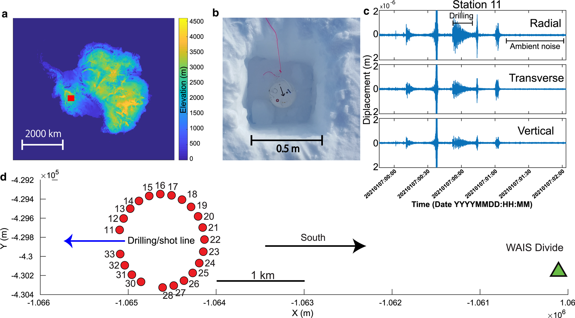
(a) Location of study area near WAIS Divide, West Antarctica. (b) Example top-down view of a Fairfield nodal seismometer placement in its shallow 0.2 m pit. The black arrow indicates the radial component alignment, and the long red string is used as part of surface flagging for later retrieval. (c) Several hours of representative three-component seismic data at station 11, featuring a combination of both natural and anthropogenic noise. (d) Map of the 22-node circular array (1 km diameter; typical station spacing of 130 m where gaps are not present) in the vicinity of WAIS Divide camp (~5 km distant, green triangle), West Antarctica, which recorded ~250 h of continuous data. Frequent drilling activity (along the blue arrow) contributed to noise on most days. Black arrow indicates geographic south. The projection here is stereographic south at a latitude of − 79.467472.

Fig. 2.

Examples of correlation beamformed data. For simplicity, we assumed plane wave incidence. (a) Beamforming of 5–10 Hz energy on 8 January, when no local human activity was present, showing a singular dominance of Rayleigh energy originating from the direction of WAIS Divide camp. Radial units are velocity, in km · s⁻¹, and angular units are clockwise degrees away from East with the same stereographic projection as Figure 1a. Black arrows are geographic North. (b) Results for 12 January, where incident energy is bimodal due to local drilling/shot activity, which occurs in a line along the Northeast. (c) 17.5–22.5 Hz result, on 8 January, showing the same beam pattern as (a), but with increased velocity. (d) Average maximum amplitude velocity picks from beamforming from 3 to 30 Hz averaged daily. (e) Average over (d), showing two clean Rayleigh modes. (f) FTAN results averaged for 8 January in 3–45 Hz for all paths within 12 degrees azimuth of WAIS Divide, showing the emergence of a third higher mode beyond 30 Hz.

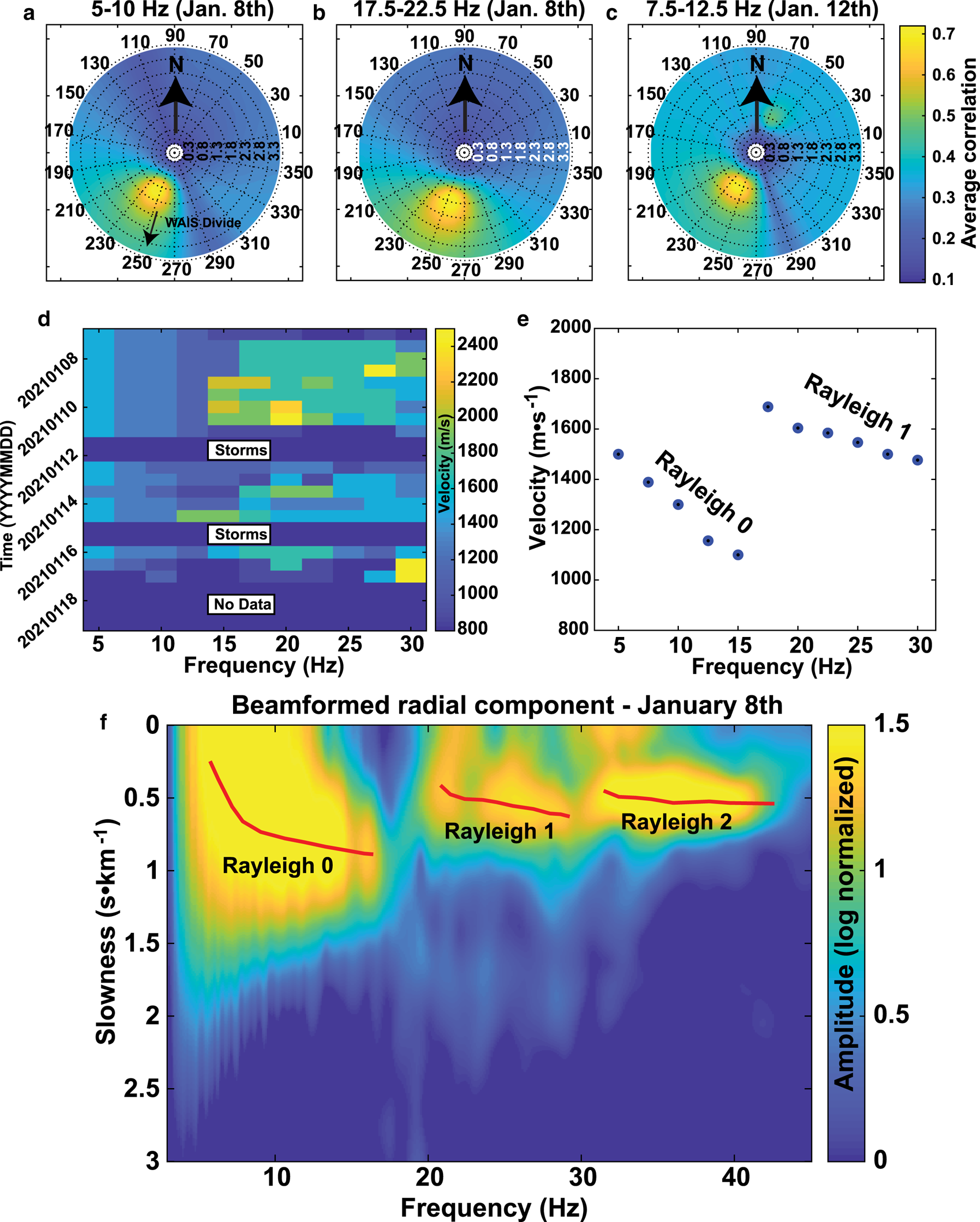
This velocity step between 15 and 20 Hz is suggestive of a surface wave modal transition in which a higher mode becomes the dominant carrier of energy. Dispersion is also observable, and particle motions are mostly limited to the radial-vertical plane at frequencies below 30 Hz, consistent with Rayleigh waves. Above 30 Hz, the noise wavefield diversifies somewhat in its angular incidence, but the azimuth continues to dominantly point in the direction of WAIS Divide camp. To more clearly visualize mode separation and transitions, we employ a frequency/slowness (FTAN) technique over horizontal ray paths within ± 12 degrees of the camp azimuth for 3—45 Hz energy (Fig. 2f). A second higher mode emerges above 30 Hz, evidenced by a distinct second modal transition. Variations in modal amplitudes could be due to varying contributions of wind noise and/or amplification/attenuation related to medium properties such as porosity.

2.3. Multi-mode particle motions

Given the extremely low velocity and layered character of firn, we approached the study of these waves noting prior results such as Ma and others (Reference Ma, Clayton and Li2016), where strong velocity transitions due to the presence of sediments resulted in a modal transition between fundamental and higher mode Rayleigh waves. In Ma and others (Reference Ma, Clayton and Li2016) the higher mode only propagated at frequencies sensitive to the basin fill, and so could be separated by analyzing its frequency-dependent particle motions. For typical seismic media, fundamental mode Rayleigh waves for Earth models have retrograde motions at the surface, whereas first higher mode Rayleigh waves (e.g. Sezawa waves; Sezawa (Reference Sezawa1935)) mostly display prograde motions.

Figure 3 shows examples of particle motions for the reconstructed correlation gather centered at 3 Hz (Fig. 3a) and 7.5 Hz (Fig. 3b) for 8 January, with the array rotated into the camp azimuth. Rayleigh particle motions for all gathers below ~18 Hz are unusually linear and inclined, with the vertical and radial components having approximately equal amplitudes and being close to in-phase. This would generally suggest P-wave energy incident at ~45 degrees, or S _V waves, but the evident dispersion and the velocity jump at 17—22 Hz are inconsistent with this interpretation. Ma and others (Reference Ma, Clayton and Li2016) suggested that inclined ellipticity, as observed here, may indicate the presence of contaminating body waves (i.e. reflected/refracted P, S _V in the firn medium; Albert (e.g. Reference Albert1998)). We briefly recap the results of the Ma and others (Reference Ma, Clayton and Li2016) derivation here. The summation of a single recorded surface wave and a body wave with arbitrary phase ϕ and frequency ω can be written as

(2)$$\left[{X \atop Y} \right] = {\bf M} \left[{\cos( \omega t + \phi) } \atop {\sin( \omega t + \phi) } \right] = {\bf U \Sigma {\bf V}}^T \left[{\cos( \omega t + \phi) } \atop {\sin( \omega t + \phi) } \right],\; $$

where M is a 2 by 2 matrix related to the amplitudes and phases of both waves and UΣV^T is the singular value decomposition of M (see Ma and others (Reference Ma, Clayton and Li2016), Appendix B). As such, if body wave arrivals exist concurrently with surface wave arrivals, we expect circular particle motions defined by [cos(ωt + ϕ),  sin(ωt + ϕ)]^T to be stretched by the Σ operator and rotated by U. Particle motion linearization is known to happen near natural S-wave structural resonance associated with shallow discontinuities, and directional body wave contamination could result in a rotation of those motions. In our case, both the radial and vertical components of motion are of similar scales for most reconstructed wave intervals in 3—18 Hz, which would imply significant body wave contamination combined with the linearization of motions due to structural resonance. This unusual phase and amplitude matching of the radial and vertical components evades any other obvious explanation, and should be the subject of deliberate future studies, should this phenomenon prove to be pervasive in firn media at higher frequencies than typically studied for imaging purposes.

Fig. 3.

Examples of longer path reconstructed correlations in the radial-vertical plane (defined by the location of WAIS Divide camp) for similar inter-stations distances at frequencies of (a) 1–5 Hz, and (b) 5–10 Hz, showing high ellipticity inclined particle motions with varying particle directions. Particle motions plotted here are normalized by the maximum of the radial component of the correlation, so their scales are arbitrary, and correspond to the associated paths in the left panels. Below 5 Hz, Love waves (transverse) are also more strongly reconstructed. These unusually linear ellipticities hold for all paths of the small array for frequencies between roughly 5 and 30  Hz, but their dispersion (Fig. 2f) precludes a purely body wave source. (c) H/V for the three picked Rayleigh modes in Figure 2f (left panel), with Rayleigh 0 exemplified here in Figures 3a,b. Rayleigh 0 above 5 Hz shows a component amplitude ratio near unity, Rayleigh 1 shows dominantly vertical amplitudes, and Rayleigh 2 features a large amplification on the radial component that displays strong evidence of spatial path dependence (right panel), indicative of variations in shallow structural layering.

2.4. Rayleigh wave H/V ratios

Along with particle motion determinations, we also estimate H/V for the three observable Rayleigh modes (referred to here as Rayleigh 0, Rayleigh 1, Rayleigh 2; Fig. 3c), calculated by picking the moveouts of obvious radial/vertical waves shown in Figure 4. In general, it is clear that the camp does indeed provide the strongest source of incoming wavefield energy, as cross-correlations are notably one sided. What this means, in terms of Eqn (1), is that the wavefield is not isotropic (i.e. it had a dominant direction), and that we are not recovering both terms in the right-hand side. Rather, we are correctly rebuilding the surface wave component for one of the two Green's function terms and little else. For frequencies between 18 and 30 Hz, there appears to be a secondary source of energy resulting in a partial reconstruction of the second Green's function term (e.g. Fig. 4, 27 Hz). This implies either a band limited source of noise such as wind, or persistently reflected waves from buried or topographic features outside the array. Though interesting, this point is left to future study.

Fig. 4.

Correlation reconstructions, and particle motion calculations for 8 January, when the dominant source of noise was WAIS Divide (see Fig. 1d). Blue, red and green seismograms are radial, vertical and transverse displacements, respectively. Only correlograms for wave paths (shown on the array subfigures) within ±12 degrees of the WAIS Divide azimuth are used. Retrograde (black ray paths) and prograde (green ray paths) particle motions are mapped to corresponding station pairs. Rayleigh wave moveouts are picked manually, and both particle motions (Fig. 3a) and H/V (Fig. 3b) are evaluated in a frequency-dependent window around the best fit moveout line.

H/V as a function of frequency is generally calculated as $\sqrt {{( R^2 + T^2) \over Z^2}}$, where R,  T,  Z are Fourier amplitude for frequency-dependent windows centered around a given moveout and are calculated for interstation paths within ± 12 degrees of the WAIS Divide azimuth (resulting in 29 paths). However, since we are isolating Rayleigh waves for paths satisfying the stationary phase criterion (i.e. pointing toward WAIS Divide camp), Rayleigh waves will be confined the P-SV plane, and corresponding Rayleigh H/V ratios simply become |R/Z|.

H/V shows strong variability across modes (Fig. 3c), with Rayleigh 0 showing an H/V near unity (e.g. Fig. 3b), Rayleigh 1 being vertically dominated, and Rayleigh 2 showing particularly elevated H/V that are clearly path dependent and with peak amplitudes that can vary by as much as one order of magnitude. We focus on Rayleigh 2, which features dominantly radial energy, particle motion linearization, and a high H/V with clear spatial variability, indicative of a relative lack of body wave contamination presumably due to source mechanisms inherent in the noise source at WAIS Divide. Mapping the smoothly interpolated H/V peaks for Rayleigh 2 to their respective paths yields a distinct pattern of lower peak frequencies in the upper portion of the array. H/V is well known to be sensitive to shallow-most structural layering (e.g. Pina-Flores (Reference Pina-Flores2016)), and is likely indicative here of firn structure variability across the array. Peak H/V is generally assumed to decrease in frequency content with a deepening first discontinuity, although isolating the specific Rayleigh modes responsible for the behavior is generally difficult when dealing with single stations. Given that we are able to isolate three distinct Rayleigh modes through cross-correlation, such an analysis is possible, and we describe it in the following section.

For noise definitively originating from WAIS Divide camp (e.g. limited to Rayleigh 0 and 1 on 8 January), we also spatially display particle motion directions and ray paths at various frequencies for WAIS near-azimuth paths. For frequencies between 5 and 15 Hz, where Rayleigh 0 dominates, we observe persistent spatially dependent transitions from retrograde to prograde motion across the array (Fig. 4, panels 2–5), and more complicated transitions for the higher modes as a function of frequency. The presence of both prograde and retrograde Rayleigh 0 waves has been previously observed in basin settings (e.g. Boue and others, Reference Boue, Denolle, Hirata, Nakagawa and Beroza2016), but this is to our knowledge the first time this has been observed to transition across such a small spatial range and at such high frequencies. Both Rayleigh 2 H/V and Rayleigh 0 particle motions share the same spatial pattern with reversed particle motions, indicative of similar structural influences, and pointing to variable near-surface structure under the array. The more chaotic appearance of particle motions of higher modes may be due to the low samples to wavelength ratio of these modes, and the quasi-linearity of radial/vertical plane motions throughout. That being said, there is a general particle motion reversal between, for example, the spatial pattern at 12 Hz and that at 33 Hz.

As a last observation, we study manifestations of recently documented firn resonance peaks (Chaput and others, Reference Chaput2018) which, unlike H/V ratios, are not relative amplifications but rather are absolute in nature and currently evade simple explanations.

3. Ambient spectral amplifications

Locally and temporally variable absolute amplifications in ambient spectra were observed here above 5 Hz, and we compare them to recently documented narrow band firn resonances first observed on Ross Ice Shelf (RIS) (Chaput and others, Reference Chaput2018; MacAyeal, Reference MacAyeal2018). Continuous passive data recorded at broadband stations deployed on RIS showed narrow band resonances that dynamically responded to environmental forcing effects on scales of minutes to months, including high-temperature anomalies and wind and accumulation-driven surface deposition/erosion effects. Although these observations showed some coherence consistent with regional weather data, stations were too isolated and distant from point weather measurements to analyze more subtle and short-term spatial and temporal variations in the seismic response. Passive data from the TIME array, however, allow more insight into this apparently widespread firn environment phenomenon, and several interesting temporal and spatial trends in peak patterns are recorded on this array.

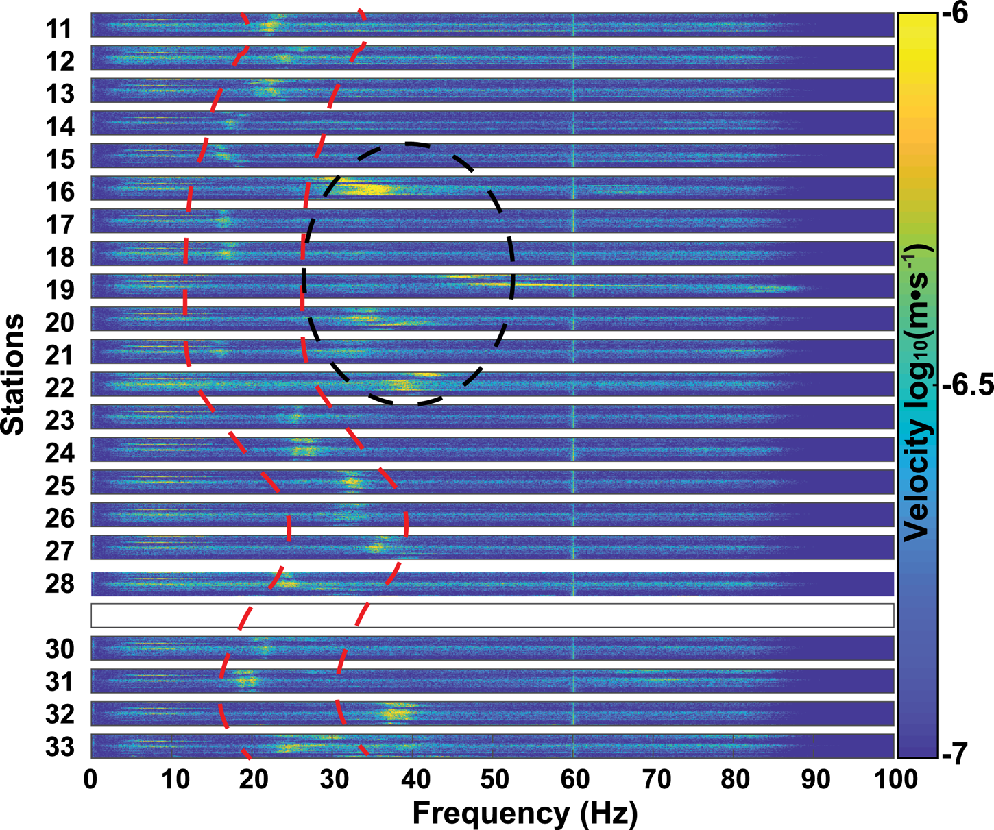
Given our circular array geometry, we are able to make a number of diagnostic observations concerning the nature of the observed frequency peaks. We first study the spatial variability of the prominent modes as a function of angular location. Figure 5 shows radial component spectrograms for the first 70 h of data at all stations. We notice that adjacent stations often have similar spectral patterns, and that there exists a roughly 2π variation pattern in the peak frequency (red dotted curves in Fig. 5). At some stations, however (e.g. 16, 20, 21, 32), the pattern jumps between adjacent stations (black dotted lines in Fig. 5), with frequency values approximately twice that of neighboring averages (i.e. a factor 2 in terms of peak frequency with respect to its neighbors). These sudden jumps suggest the excitation of a higher harmonic. The smooth spatial variability of the lower pattern, interrupted by the occasional higher jump, suggests a sensitivity to firn structure variability over the array aperture, as also indicated by other observations noted in previous sections. For instance, if these resonances are sensitive to shallow structure (in the H/V sense), then a 2π variability would imply an approximate 2D dipping plane in terms of structure across the array. We evaluate this hypothesis in the following section. A persistent 60 Hz peak is recorded uniformly across the array, which we attribute to electrical power generation and use at WAIS Divide camp.

Fig. 5.

Depiction of spectral peak spatial variability around the circular array (interstation spacing is 130 m, aside from the gap at nonfunctional station 29). Each spectrogram presents the first 70 h of data (the compressed vertical axis of each spectrogram) where resonance peaks were stable, before significant storm activity perturbed them. A roughly 2π peak azimuthal trend can be observed in the center frequency for the lower of the prominent peaks, and several stations feature a higher, stronger peak that may be a harmonic. The stable peak at 60 Hz is attributed to the AC generator at WAIS Divide camp.

To ensure that these observations are indeed part of the temporally varying and environmentally linked phenomena documented by Chaput and others (Reference Chaput2018) on the Ross Ice Shelf, we examine the spectral peak patterns in terms of temporal variability with respect to weather. As in Chaput and others (Reference Chaput2018), we discount instrument resonances as the root cause of these spectral peaks, given that the nodal seismographs are buried and have been tested for such behavior in a laboratory setting (i.e. Ringler and others, Reference Ringler, Anthony, Karplus, Holland and Wilson2018). Two broad observations further support this notion:

1. 1) The seismic nodes were (shallowly) buried at depths of ~0.2 m, and remained so for the duration of recording. Temperatures remained significantly below freezing, precluding node exhumation due to local wind/instrument coupling or freeze/thaw effects (as observed, for instance, by Johnson and others (Reference Johnson, Vernon, Nakata and Ben-Zion2019)).

2. 2) These patterns of resonances and their response to environmental forcing, summarized in Chaput and others (Reference Chaput2018), are observable across a variety of instrumentation configurations and sites, with both nodal and broadband instruments, and with and without surface flagging. Spectral peaks furthermore show spatial coherence on small to intermediate scales (e.g. Fig. 5) that preclude the possibility of individual instrument coupling or resonance effects, which would produce spatially random or spatially identical patterns.

Figure 6 shows three-component spectrogram segments compared with the gradient of the wind azimuth θ times the square of the wind speed V _w (to identify intervals of both strong winds and changing wind direction) and wind speed. The following observations are noted:

1. 1) Resonance peaks are in general visible on all three components, but are stronger on the horizontals often by up to an order of magnitude in amplitude (although this is variable).

2. 2) A resonance peak may show ‘splitting’, where peak doublets are observed that vary proportionately in frequency with time and show up to 15% peak frequency differences. In such cases, split peaks are typically recorded on both the vertical and horizontal components, possibly reflecting anisotropic structure (e.g. Fig. 6a).

3. 3) Storm events with blowing snow (noted in field notes by days with very low visibility) were associated with frequency shifts by Chaput and others (Reference Chaput2018). Peaks are also observed to sometimes drift in frequency with changes in wind azimuth (Fig. 6b).

4. 4) Peaks are sensitive to temperature anomalies, and will slowly decrease in both frequency content and amplitude with persistently high surface temperatures and may fluctuate daily even if temperatures approach freezing.

5. 5) Peak patterns also occasionally show evidence of harmonic behavior following storm events (Fig. 6c).

Fig. 6.

Examples of temporally varying narrow-band signals across time intervals of several days (note differing duration and frequency range). (a) Spectral splitting of resonance peaks, showing clear S _V mapping of both peaks. (b) Example of the potential impact of wind direction and forcing, showing changes that coincide with periods of rapid changes in wind azimuth θ times the square of wind speed V _w (red lines). Changes in site response during such intervals may also potentially be affected by snow deposition or scouring. (c) Transient harmonic behavior (red dotted box) following a storm sequence (black dotted lines). Red line designates another period of high wind azimuthal gradient with corresponding peak drift. Although some of these behaviors are corroborated at adjacent stations, many such effects are observed to be station-specific on the length scale of the station spacing (130 m).

The persistent mapping of energy onto all three components, the addition of splitting on the horizontals, and the increase of amplitude corresponding to higher wind speeds, suggest a P − S _V resonance excitation from a wind source. Although we cannot discount the possibility of S _H resonances being excited as well, they are not observed conclusively on the TIME array, as indicated by the mapping of peaks onto the vertical component even in cases of peak doublets. The increase in peak frequency content with the passing of storms is intriguing, and Chaput and others (Reference Chaput2018) hypothesized that multiple processes could account for this. Jumps in frequency content occur as winds are dying down and have time scales as short as a few hours. Two mechanisms were proposed, namely a change in surface coupling structure through deposition and stripping of surface material, and the rapid post storm formation of wind slab, a denser, more rigid layer of snow with low porosity several centimeters in thickness. Using 1.5D numerical simulations limited to flat layers with realistic firn velocity models, Chaput and others (Reference Chaput2018) were able to show that both mechanisms could produce an upward shift in frequency content, although no 2D or 3D effects were explored. Surface wave amplification effects were also noted by Dal Moro (Reference Dal Moro2020), who studied the effect of a thin, stiff layer overlaying a low velocity medium. In particular, higher mode Love waves were numerically shown to strongly emerge as harmonics with the presence of a stiff thin surface layer, a behavior potentially observed in Figure 6c, despite its mapping to the vertical component. A thorough numerical exploration of these various effects, particularly concerning deposition and temperature, can be found in Chaput and others (Reference Chaput2018).

As a further test of spatial variability, we roughly interpolate the lowest spectral peaks in Figure 5 according to the red lines, while making the assumption that the higher peaks noted by the black dotted ellipse are factor 2 harmonics of the peaks noted at nearest neighbors. These inferred peaks are then mapped to their respective stations and are compared with H/V and Rayleigh 0 particle motions (Fig. 7). Notably, a cluster of lower frequency peaks appears to map to the upper portion of the array in the same manner as lower frequency H/V peaks (Rayleigh 2) and prograde particle motions (Rayleigh 0), suggesting that surface wave effects may also be responsible for these amplifications. The first two effects, particle motions and H/V ratios for individual Rayleigh modes, can be numerically studied, and we do so in a 1D manner in the following section. Resonance peaks, however, have not been definitively constrained in terms of source/structure interaction. Thus, we subsequently explore several possibilities accounting for both SV plane polarization and the smooth spatial variation shown in Figure 5.

Fig. 7.

Peak interpolated resonance frequency (for values between red dotted lines in Fig. 8) mapped spatially compared with example Rayleigh 0 particle motions (Fig. 4, 12 Hz) and peak H/V frequency (Fig. 3b). The red dotted line indicates a coherent pattern of lower frequency resonances that is spatially correlated with both prograde Rayleigh 0 particle motions and lower H/V peak frequency for Rayleigh 2.

4. 1D numerical simulations

We seek to test the extent to which realistic near-surface velocity models can convincingly simulate the surface wave phenomenology observed here.

For 1D velocity and density profiles, pseudo-analytical methods for rapidly obtaining sensitivity kernels and other seismic properties are provided by several publicly available packages. We made use of RAYLEE (Haney and Tsai, Reference Haney and Tsai2015, Reference Haney and Tsai2017), a finite element model for surface wave simulation and inversion written in MATLAB©.

Firn densification processes on average tend to follow generally predictable velocity and density profiles controlled by their regional environments. For instance, compaction and ablation processes have been broadly studied in Antarctica, and firn profiles on average were modeled as having similar characteristics for RIS and WAIS Divide regions (van den Broeke, Reference van den Broeke2008). Local variations, however, can be severe and diverge significantly away from steady-state assumptions (e.g. Ligtenberg and others, Reference Ligtenberg, Helsen and van den Broeke2011; Reeh, Reference Reeh2008) owing to the formation of ice lens layers, hoar frost and other atmospherically driven structures. Given that a high-resolution seismic model is not yet available for this area, though such preliminary efforts are in progress as per Adam Booth (pers. comm. 2021), we proceed as follows. We begin with a smooth firn velocity model obtained from inversion of anthropogenic (camp noise) 4–18 Hz Rayleigh and Love waves recorded on the Ross Ice Shelf by a small-aperture (5 km nonuniform spacing) short-period seismic array (Diez and others, Reference Diez2016). Although likely not an exact average match to our site, perturbations of this model allow us to investigate variability in Rayleigh wave sensitivity kernels and eigenvalues in such media.

We investigate two main types of perturbations away from our starting firn model:

1. 1) A series of smooth slowing perturbations for the firn profile, and

2. 2) a series of low-pass filtered random Gaussian noise perturbations applied the initial firn profile.

We seek here to model several observations: the reversal of particle motions in Rayleigh 0; the specific pattern of H/V perturbations for all three modes; the likelihood that a planar deepening of firn structure across the array could account for spatial variations thereof.

The first set of perturbations seeks to gauge the impact of average firn structure variations on surface waves, given that the starting model from Diez and others (Reference Diez2016) may, on average, be slightly slower or faster than at our study site, and variable within the aperture of our array. Specifically, particle motion reversals observed in Figure 4 for the Rayleigh 0 mode should be sensitive to these forms of perturbations given the generally more broad nature of fundamental mode kernels. The second set of perturbations seeks to study the effect of severe shallow ‘switch backs’ (i.e. fast/slow/fast and similar transitions) in the top 10 s of meters of the firn, suspected here to be largely responsible for H/V amplifications of the second Rayleigh mode given its variation in peak frequency over a small spatial scale.

To examine particle motion directions, we adopted the convention of Tanimoto and Rivera (Reference Tanimoto and Rivera2005), whereby the radial eigenfunction is negative and, in the absence of a firn layer and in the majority of Earth media, fundamental Rayleigh particle motions are retrograde. For each perturbed profile, we computed the ZH ratio, defined by ZH = U(R)/(1.5 · V(R)), where U(R) and V(R) are the vertical and horizontal eigenfunctions (Takeuchi and Saito, Reference Takeuchi and Saito1972; Tanimoto and Rivera, Reference Tanimoto and Rivera2005), as a proxy for determining frequency ranges over which particle motion reversals can occur. A positive ZH implies prograde motions, whereas a negative ZH indicates retrograde motions. Similarly, the H/V ratio for a given Rayleigh mode can be calculated by the absolute value of the ratio of its radial to vertical eigenvalues, and so is closely related to the ZH ratio. It is primarily used as a metric sensitive to near-surface discontinuities, and higher mode Rayleigh waves here are obvious candidates for study.

For both types of perturbations, we generate H/V ratios, ZH ratios (indicative of particle motion directions) and depth sensitivity kernels for all modes, which provide additional information concerning potential mechanisms for spectral amplifications (Figs 5 and 6) and allow us to consider which portions of the firn are primarily sampled by surface waves.

Figure 8a shows the results of smoothly slowed firn profiles, starting with the RIS profile computed by Diez and others (Reference Diez2016). It should be noted here that ‘sped up’ versions of this profile did not result in zones of particle motion reversal for Rayleigh 0, and as such are not shown here. As velocity profiles move from faster to slower, a region of prograde Rayleigh 0 motion emerges that narrows and shifts to lower frequencies (Fig. 8a, bottom panels). These results would suggest at first glance that our firn profile at WAIS Divide is necessarily slower than the one on RIS given the emergence of a zone of prograde motions for models 3–10, perhaps due to different firn densification conditions (as per van den Broeke (Reference van den Broeke2008)). We can however note that the corresponding H/V ratios for this region are not equivalent to those observed in our data (i.e. a near-unity H/V for Rayleigh 0, a vertically dominated Rayleigh 1 and large values for Rayleigh 2). In short, broadly slowing down the firn profile tends to result in higher H/V ratios for Rayleigh 0, and this is not observed, though, as discussed previously this could also be due to contamination of Rayleigh 0 by body waves. We anticipate that more random and severe perturbations to these profiles exist, and thus subsequently perturb the profile in a different manner.

Fig. 8.

H/V and ZH ratios obtained from finite element modeling of surface wave eigenvalues (RAYLEE). Positive values for ZH indicate prograde particle motions, and negative values indicate retrograde motions. Large values of H/V indicate horizontally dominated Rayleigh waves, and values of < 1 indicate vertically dominated Rayleigh waves. (a) Results for 10 progressively slowed firn profiles. Black lines indicate the base firn model. (b) Results for 10 low-pass Gaussian noise perturbed velocity profiles. As in (a), the black lines indicate base firn models. Model 8 is used as an example for further study.

Figure 8b shows the results of ten models produced by adding low-pass filtered additive Gaussian perturbations to the initial RIS profile, with decreasing standard deviation as a function of depth, as is expected from densification processes. The amplitude of the perturbations was chosen arbitrarily to qualitatively mirror non-steady state densification models (Ligtenberg and others, Reference Ligtenberg, Helsen and van den Broeke2011). It is immediately clear that a large degree of variability, particularly in H/V ratios for Rayleigh 2, can be imparted into surface wave eigenvalues by severe shallow variations in structure without slowing the profile on average. ZH ratios for Rayleigh 0, although clearly variable over different perturbed models, never become positive for any of the models in Figure 8b, nor do ZH ratios for Rayleigh 1 become negative, suggesting that a slight slowing of the profile from the base model is indeed additionally required to account for our observations. Several of the random models (1,3,7 in Fig. 8b, Rayleigh 2 H/V) show that high values of H/V can be obtained in the 30–50 Hz range for Rayleigh 2, while maintaining near unity H/V for Rayleigh 0 and < 1 for Rayleigh 1. These realistic random models thus capture fine scale high-frequency effects related to the propagation of multi-mode Rayleigh waves, but also underscore the inherent difficulty in performing a unique structural inversion for the firn based on these data. A combination of the two perturbations is likely here (i.e. a slower average profile, and a set of random but severe perturbations), but a joint inversion of these quantities is beyond the scope of this paper.

We now turn our attention to the spatial variability inherent in our observations and in particular, the implication of a shift in H/V for Rayleigh 2 over the small aperture of our array. GPR studies at other Antarctic firn sites have revealed the presence of modulations in firn layering with scales of 100 s of m to 10 s of km (e.g. Sinisalo and others, Reference Sinisalo, Grinsted, Moore, Karkas and Pettersson2003; Arcone and others, Reference Arcone, Spikes and Hamilton2005a, Reference Arcone, Spikes and Hamilton2005b). Whether these observations are pervasive throughout Antarctic firn is unclear, but we anticipate that semi-planar modulations of firn layering over scales of 100 s to 1000s of meters are possible at our study site. We may not necessarily expect to be able to concurrently model a spatial reversal in ZH for Rayleigh 0 while also ensuring that its H/V remains near unity, given the inherent relationship between the two metrics (e.g. a particle motion reversal implies a zero crossing in ZH ratios, which results in either amplified or near-zero H/V) and the likely contamination from body waves as discussed in previous sections. If body wave contamination is indeed present, as we suspect, then a particle motion reversal as observed in Figure 4 is possible without a resulting H/V pole or zero. From the three random models that qualitatively produce Rayleigh 2 H/V in the right range, we choose model 7 (Fig. 8) as a base, and shift the pattern of random perturbations downward along initial firn profile for the RIS. Figure 9 shows the impact of such a structural downward shift on H/V and ZH for all three modes. The H/V peak at around 40 Hz for Rayleigh 2, for instance, can be moved downward significantly with a small linear shift in structure without affecting Rayleigh 0 or Rayleigh 1. The ZH ratio also shows a modest shift for Rayleigh 0 toward a zero crossing, suggesting that such a shift, if combined with a slightly slower firn model on average, could be just enough to cause a particle motion reversal. As such, there is strong evidence that a locally planar dipping firn structure on the order of a few meters is present under our array, deepening from bottom to top in Figure 7 (i.e. west to east), which would account for the 2π variations in H/V and particle motions noted in Figure 7b,c.

Fig. 9.

(a) Effect on multimode Rayleigh H/V of a small (2 m) downward shift of model 7 in Figure 8c. (b) Resulting variations in ZH. (c) Base and shifted velocity models used in (a, b).

The final point to address here is more speculative and relates to the absolute amplifications observed in Figures 5 and 6. Unlike the observations we have modeled thus far, these spectral amplifications do not currently have a well-described source model despite initial attempts by Chaput and others (Reference Chaput2018). There are two modes of variability for these peaks: spatial (structural) and temporal (source and structure). Given that source studies would likely require high-resolution atmospheric and surface data (such as time lapse photogrammetry to study wind coupling locales), we focus here on structural variability and explore possible excitation mechanisms. Wave resonance mechanisms must account for the P-SV polarization of peaks and their similar sensitivity to spatial variation in firn structure as Rayleigh waves (Fig. 7). Given the novelty of these absolute spectral amplifications, we discuss them in terms of two possible mechanisms, and weigh them with respect to the evidence: S _V resonances and relative Rayleigh wave amplification. Given that we favor the latter, discussion concerning S _V resonances can be found in the online Supplementary material.

4.1. Surface wave resonances

Rayleigh and Love wave amplifications due to interactions with basin structures do not have closed form solutions beyond simple 1D approximations. Studies targeting surface wave amplification without resorting to strong motion seismograms generally follow a relative calculation, with one nearby station deployed over bedrock with a known velocity profile serving as a benchmark. Initial works by Tromp and Dahlen (Reference Tromp and Dahlen1992), expanded upon by Brissaud and others (Reference Brissaud, Bowden and Tsai2020), Bowden and Tsai (Reference Bowden and Tsai2017), and Feng and Ritzwoller (Reference Feng and Ritzwoller2017) have made use of broadly available ambient noise velocity maps of the continental US to predict and study amplifications in known basin structures while accounting for basin edge effects. Tromp and Dahlen (Reference Tromp and Dahlen1992) initially formulated relative amplification A _n with respect to a reference site $A_n^R$ as:

(3)$${A_n\over A_n^R} = {u_n( 0) \over u_n^R( 0) }\left({Ul_0\over U^Rl_0^R} \right)^{-1/2}.$$

Here, u _n(0) and $u_n^R( 0)$ are the displacement eigenfunctions at the surface for the reference and basin sites, n = 1,  2,  3, and U is group velocity. l ₀ is an integral over eigenfunctions and density ρ and depends on the wave type. For Rayleigh:

(4)$$l_0 = \int_{0}^{\infty}\rho( z) \left(u_1( z) ^2 + u_2( z) ^2 \right){\rm dz}$$

and for Love:

(5)$$l_0 = \int_{0}^{\infty}\rho( z) u_3( z) ^2 ~ {\rm dz} ~ .$$

We should note that this approach is useful, but is limited to 1D relative effects, and information pertaining to absolute amplification cannot be resolved (but can serve as a relative indicator of amplification in some cases). In our case, we consider the 20 models discussed in the previous section, with a ‘base model’ consisting of RIS profile. The first tenmodels consist of homogeneous slowing functions, and the last ten models consist of the RIS model with random additive Gaussian noise. Figure 10 shows the resulting relative amplifications for the first three Rayleigh modes observed in our data. Note that the frequency range that can be resolved is largely determined by the reference model (i.e. a much faster reference model may yield larger relative amplifications, but higher modes will not propagate at lower frequencies). Two primary effects are noted:

1. 1) Large amplifications are possible with slower firn profiles (Fig. 10a), as expected, and Rayleigh 0 and 1 have similar amplifications (i.e. Vertical ~ Radial). Rayleigh 2, however, exhibits disjointed radial and vertical amplifications, with a large radial dominance near 20 Hz and a large vertical dominance near 50 Hz. Large H/V ratios are indeed a feature of spectral peaks in Figure 5, which is intriguing, and although we do see radial-only amplifications at many frequencies, the models also predict vertically dominated modes at some frequencies, and this point is not observed in the data.

2. 2) Figure 10b shows examples of firn profiles containing the random noise perturbations. Amplifications relative to the initial profile are more modest, but display a wide range of behaviors, particularly in the higher modes. Interestingly, stronger discontinuities in themselves do not guarantee higher relative peaks, as extreme shallow gradients are present in the noisy models relative to the base, but we are limited in terms of interpretation by the relative aspect of these calculations.

Fig. 10.

(a) Relative Rayleigh amplifications with respect to 10 progressively slowed firn velocity profiles (right panel). (b) Same as (a), except for 10 low-pass Gaussian noise perturbed velocity profiles. (c) Similarly to Figure 9, model 8 is perturbed by shifting the perturbation pattern downward by 2 m, and the resulting amplification of the Rayleigh 0 is calculated for both profiles (right panel).

Under this source interpretation, we may as before study the impact of shifting a random structure downward to see if a given amplification can also translate in frequency. As such, we choose an example model that has resulted in a peak in the − 20 to 30 Hz range (we arbitrarily choose model 8), which has a modest peak at ~ 25 Hz, and study the effect of a 2 m downward shift in the profile perturbations. As exemplified by Figure 10c, the resonance shifts slightly to lower frequencies. Although it agrees with H/V response, we do not consider this to be generally diagnostic, given the complexity of firn resonance phenomenology and the source-independent nature of these computations. Rayleigh wave amplifications can be obtained this way with a variety of plane polarizations, and it is thus clear that source excitation (as also inferred by Chaput and others (Reference Chaput2018)) plays a critical role in the generation of these features. As such, although this formulation is only a relative approximation that certainly does not capture the complexities of features shown in Figures 5 and 6, it may offer a glimpse into the structural aspect of firn that allows these resonances to occur.

We view Rayleigh wave amplification as an intuitive candidate here to describe much of the firn ambient seismic wavefield, given the likely P − S _V dominant excitation of wind noise, the relationship between wind and peak drift and the complex behavior of anthropogenically excited Rayleigh waves noted in this study. Although a more detailed nature of these amplifications is difficult to model and interpret, the P − S _V plane constraint on these resonances presents intriguing opportunities such as potential sensitivity to azimuthal anisotropy at single stations, which, in general, is not possible with ambient noise measurements without time domain reconstructions. Finally, the spatial mapping of Rayleigh 0 particle motions (and conversely, the approximate reverse mapping for Rayleigh 2) combined with a similar trend in H/V and resonance peak estimates (Fig. 7) all suggest sensitivity to similar structures, which reinforces the notion of surface wave amplification. In particular, H/V peak frequency, largely acknowledged to be a result of Rayleigh wave motion linearization, also maps to decreasing resonance peak frequency, suggesting a direct link between the two processes. We provide further discussion of alternate S _V explanations and the potential impact of multi-mode depth sensitivity kernels in the online Supplementary material.