2. Problem formulation

We follow [Reference Dyachenko, Kuznetsov, Spector and Zakharov9, Reference Semenova and Byrnes34] and use the conformal mapping reformulation of the water wave problem. This reformulation views the parameterization of the surface $(x(u,t),y(u,t))$ as the real and imaginary parts of a conformal mapping $z(w)$ from the upper boundary of a rectangular domain $w = u + iv$ of known width $2\pi$ and height $h$ in the complex plane, see Figure 2. The velocity potential along the surface is defined as $\psi(u,t) = Re [\Pi(u,t)]$, using the complex potential $\Pi(w,t) = \phi(w,t)+i\theta(w,t)$.

Figure 2. The mapping $z(w,t)$ from the conformal domain (right) to the physical domain (left). The free surface of the physical domain $(x(u,t),y(u,t))$ is parameterized as a function of the top surface of the conformal domain $w = u + i0$.

Using this reformulation, the four explicit PDEs posed on an evolving domain with a free boundary (1–4) become the pair of non-local, implicit PDEs posed on the interval $[-\pi,\pi]$ given by

(5)\begin{equation} y_tx_u-x_ty_u = - \hat{R}\psi_u, \end{equation}

(6)\begin{equation} \psi_t y_u - \psi_u y_t = - gyy_u - \hat{R}(\psi_t x_u - \psi_u x_t + gyx_u). \end{equation}

Here $\hat{R}$ is a generalization of the periodic Hilbert transform, which depends on the height $h$ of the conformal domain:

(7)\begin{equation} \hat{R}f(u) = \frac{1}{2h} \int{\kern-12.6pt}-_\mathbb{R}\frac{f(u')}{\sinh(\pi (u'-u)/2h)}du', \end{equation}

where $\int{\kern-12.6pt}-_\mathbb{R}$ is the principal value integral over the real line. To apply this operator using the Fast Fourier Transform, we use

(8)\begin{equation} (\hat{R}f)_k = i\tanh(kh)f_k, \end{equation}

where $f_k$ is the $k$-th Fourier mode of $f(u)$, see [Reference Zakharov, Kuznetsov and Dyachenko42]. The operator $\hat{R}$ has an inverse $\hat{T}$, see [Reference Zakharov, Kuznetsov and Dyachenko42], given by

(9)\begin{equation} \hat{T}f = \frac{1}{h} \int{\kern-12.6pt}-_{\mathbb{R}} \frac{f(u')}{1-e^{-\pi(u-u')/h}}du'. \end{equation}

In Fourier space, this operator is applied using

(10)\begin{equation} (\hat{T}f)_k = -i\coth(kh)f_k. \end{equation}

Defining the operator $\hat{K} = \hat{T} \partial_u$ and moving into a travelling frame with speed $c$, we find that the surface wave profile satisfies the Babenko equation

(11)\begin{equation} 0=\hat{S}y = (c^2\hat{K}-g)y-g\left(y\hat{K}y+\frac{1}{2}\hat{K}y^2\right). \end{equation}

Here $\hat{S}$ is the finite-depth generalization of the Babenko operator discussed in [Reference Semenova and Byrnes34]. The surface elevation $y$ is related to the velocity potential $\psi$ through

(12)\begin{equation} cy_u=\hat{R}\psi_u. \end{equation}

Our primary concern is the accurate solution of the Babenko equation  $\hat{S}y = 0$ for a fluid of fixed physical depth.

The Hamiltonian of the system (1–4) is also its total energy,

(13)\begin{equation} \mathcal{H} = \frac{1}{2} \int_{-\pi}^{\pi} \psi \hat{G}(\eta)\psi\,dx + \frac{g}{2}\int_{-\pi}^{\pi} \eta^2\,dx, \end{equation}

where $\hat{G}(\eta)$ is the Dirichlet-to-Neumann operator [Reference Craig and Sulem5, Reference Zakharov43]. In conformal variables, the Hamiltonian is written as

(14)\begin{equation} \mathcal{H} = -\frac{1}{2}\int_{-\pi}^{\pi}\psi \hat R \partial_u \psi du +\frac{g}{2}\int_{-\pi}^{\pi}y^2x_udu, \end{equation}

with Dirichlet-to-Neumann operator $-\hat R \partial_u$, see [Reference Dyachenko, Kuznetsov, Spector and Zakharov9] for details.

3. Computing waves in a fixed depth: numerical method

Following Dyachenko et al. [Reference Dyachenko, Lushnikov and Korotkevich13, Reference Semenova and Byrnes34] in infinite depth, we compute the Stokes waves using a Newton-Conjugate-Gradient method. Waves with a fixed conformal depth $h$ are computed in [Reference Semenova and Byrnes34]. This method will not be expounded upon in this paper. Instead, we extend the application of the method in [Reference Semenova and Byrnes34] to the computation of Stokes waves in two ways.

• • We use the method of [Reference Semenova and Byrnes34] to compute waves of a fixed physical depth $d$ instead of a fixed conformal depth $h$. Zakharov et al. [Reference Zakharov, Kuznetsov and Dyachenko42] demonstrate that $h$ and $d$ differ for non-flat surfaces, see also Dyachenko & Hur [Reference Dyachenko and Hur10]. They are related by the average of the wave’s surface elevation $y$ through

  (15)\begin{equation} h = d + \langle y \rangle. \end{equation}

  As in [Reference Dyachenko and Hur10], $\langle \cdot \rangle$ denotes the average over a single period of the conformal variable $u$ instead of over physical space $x$. To compute a family of waves in water of physical depth $d=D$, for each value of the speed $c$, we choose a value of the conformal depth $\tilde{h}(c) \gt 0$ so that (15) gives

  (16)\begin{equation} E(c;\tilde{h},D) = D + \langle y(\tilde{h}(c;D),c) \rangle - \tilde{h}(c;D) = 0. \end{equation}

  Here, $E(c;h,D)$ measures the difference between the desired value of the physical depth $D$ and the actual value of the physical depth when $h$ is chosen as the conformal depth. When $E(c;h,D)=0$, we find the correct value of the conformal depth $h$ to ensure the resulting wave has the desired value of the speed $c$ in physical depth $D$.

  To determine the value $h(c;D)$ that gives rise to a wave travelling at speed $c$ in water of depth $D$, we use a bisection algorithm. We compute a wave and with it the value $E(c;h,D)$ at each step, terminating the calculations once sufficient accuracy (we choose $10^{-11}$ in our computations) is attained. Next, we use the value of $h$ found to compute a wave with the desired speed $c$ and physical depth $D$. A plot of a few Stokes waves of varying steepness in depths 0.1, 1 and 10 is shown in Figure 3. Figure 4 shows the waves in depth 0.1 from Figure 3 in more detail.

  

  Figure 3. Waves of increasing steepness in depths 0.1 (bottom), 1 (middle) and 10 (top). All waves are plotted with an accurate aspect ratio. Note that in each case, a corner with an included angle of 120 degrees forms at the crest. In depth 0.1, the wave localizes to a fraction of the wavelength, reminiscent to a solitary wave. The wave in depth 0.1 is difficult to see at this scale, see Figure 4.

  

  Figure 4. Waves of increasing steepness in depth 0.1. The top two panels are plotted with accurate aspect ratios, with the middle panel being a zoom of the central unit interval of the period to showcase the similarity to the full period of waves in deeper water. The bottom panel has been stretched in the $y$ direction to show the localization of the wave and its profile.

  Alternatively, one could use Newton’s method to solve (16). This requires the computation of $\partial E/\partial h$. To this end, we compute $\partial y/\partial h$, obtained from a derivative of the Babenko equation (11) with respect to the parameter $h$ and solving the resulting equation for $\partial y/\partial h$. This requires the inversion of the linearization of $\hat{S}$ about $y$, and hence the use of MINRES at each step of Newton’s Method. Although Newton’s method requires fewer iterations than does bisection, this added use of MINRES substantially increases the cost of each Newton step. The bisection method described above is more efficient, even more so as steeper waves are computed. These computations could be carried out using a secant method, although any improvements are likely to be moderate, since a relatively small number of bisection steps are needed, ranging from 4 to 20.

  As noted in previous works [Reference Deconinck and Oliveras8, Reference Semenova and Byrnes34] and shown in Figures 3 and 4, in shallow water, high-amplitude Stokes waves become increasingly localized within their wavelengths. To measure this localization, we first determine the height of half width of an extreme wave in deep water, as a proportion of the full amplitude of the wave. Then, the width of an extreme wave in a shallower fluid at the height which is the same fraction of the full amplitude gives a measure of the localization of that wave. In particular, dividing the full period by double this width gives a modified wave number $\tilde{k}(d)$ for the extreme waves in that depth, which accounts for their localization. (To measure the width of half height of an extreme wave in deep water, we use the steepest computed wave in a depth 10 fluid. This serves as a good proxy for an extreme wave in infinite depth, as the Fourier signs of the operators in Equation (11) differ from the infinite depth problem by less than $10^{-6}\%$ at this depth.) A sample wave in depth 0.5 is shown in Figure 5, and the change of the modified wave number as a function of depth is shown in Figure 6. Interestingly, this is approximated well by an inverse power of a shifted hyperbolic tangent, also shown in Figure 6. Other functions that approach zero linearly as their argument tends to zero and one as their argument tends to infinity could have been used with similar relative errors. However, the hyperbolic tangent offers a connection with the dispersion relation $\omega(k,d)^2=k\tanh(kd)$ with the wavenumber $k$ set to 1. This connection with the dispersion relation is intriguing, given the connection between the behaviour of the dispersion relation and the limiting waves in the context of simpler fluid models [Reference Ehrnström, Mæhlen and Varholm15, Reference Enciso, Gómez-Serrano and Vergara16].

  

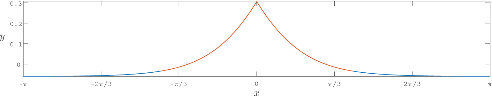
  Figure 5. Profile of the steepest computed wave in depth $d = 0.5$. Blue shows the full period of the wave, whereas red shows the localization of the wave within the period, i.e., it shows the portion of the wave that is not small. As depth decreases, the width of the red curve shrinks relative to the period, as shown in Figures 3 and 6.

  

  Figure 6. Top: change in the modified wave number $\tilde{k}(d)$, and fit to $1.06(\tanh(1.01d))^{-0.989}$ where the exponent includes $-$1 in its confidence interval. The errors in the fit are two orders of magnitude smaller than the value of the modified wave number. Data for the modified wave number is a solid blue line, and the fit is a dashed blue line.

• • A second extension of our work is the execution of these computations in variable-precision arithmetic. For these waves, Julia’s BigFloat class [Reference Bezanson, Edelman, Karpinski and Shah3] is used to solve the Babenko equation  $\hat{S}y=0$ with a tolerance of $10^{-64}$, i.e., the computed value of the $2$-norm satisfies

  (17)\begin{equation} \|\hat{S}y\|_2 \lt 10^{-64}. \end{equation}

  Applying this precision increases the costs of the computations significantly and a full exploration of finite-depth Stokes waves with this accuracy will have to wait until the development of a more refined method, discussed briefly at the end of this section as well as in Section 5. Any computations that rely on these waves are mentioned explicitly. All other computations are performed using Matlab in double precision.

Since our method is based on a pseudo-spectral method, the application of all operators enjoys spectral accuracy. The convergence of our method is verified by the residuals of the Babenko equation becoming small, starting around $10^{-14}$ for small waves and eventually reaching errors not exceeding $10^{-10}$ for the steepest waves. This accuracy loss grows proportionately to $(\mathcal{S}_{max}-\mathcal{S})^{-1.5}$ where $\mathcal{S}_{max}$ is the steepness of the tallest computed wave. Such growth is connected to the approach of a pair of square-root type branch points to the computational domain, discussed in Section 5. In particular, we require an increasing number of Fourier modes to accurately represent the solution $y$ and the operators in $\hat S$ as this branch point approaches, leading to the accumulation of numerical errors. The growth of these errors with the number of Fourier modes as we approach the steepest wave is shown in Figure 7. To compute waves nearer to the limiting wave, one may be able to follow the work of Lushnikov et al. [Reference Lushnikov, Dyachenko and Silantyev26] and Dyachenko et al. [Reference Dyachenko, Hur and Silantyev11] in infinite depth, using an auxiliary conformal mapping to push the singularities further from the conformal domain.

Figure 7. Log-log plot of residuals and number of Fourier modes as a function of steepness. The solid blue line shows the residuals $\|\hat{S}y\|_2$, the dashed red line shows a rescaled number of Fourier modes and the purple dashed-dotted line is proportional to $(\mathcal{S}_{\lim}-\mathcal{S})^{-1.5}$. The growth of the $L^2$-norm of the residuals is directly related to the number of Fourier modes. Both grow approximately proportionally to $(\mathcal{S}_{\lim}-\mathcal{S})^{-1.5}$.

4. Oscillations in energy and wave speed

Longuet-Higgins and Fox [Reference Longuet-Higgins and Fox24, Reference Longuet-Higgins and Fox25] give asymptotic results relating the profile of a near-limiting wave in infinite depth, as well as its energy and wave speed, to a perturbation parameter $\epsilon$ related to the radius of curvature of that wave. Their perturbation parameter $\epsilon$ is defined as

(18)\begin{equation} \epsilon = \frac{s}{c_0\sqrt{2}}, \end{equation}

where $s$ is the particle speed at the crest of the travelling wave, and $c_0$ is the phase speed given by the dispersion relation

(19)\begin{equation} \omega^2(k) = gk\tanh(kd). \end{equation}

In particular, Longuet-Higgins and Fox found that the speed of a near-extreme Stokes wave changes as

(20)\begin{align}c^2 &\sim \frac{g}{k}\left(c_{\lim}^2+a_2\epsilon^3\cos(3\mu\ln(\epsilon)+a_4)\right) + \ldots \nonumber\\ &\sim \frac{g}{k}\left( 1.1931-1.18\epsilon^3\cos(2.143\ln(\epsilon)+2.22)\right)+\ldots .\end{align}

Here $c_{\lim}$ is the speed of the extreme wave. Similar expansions are given for the kinetic energy $T$ and potential energy $U$:

(21)\begin{align} T &\sim T_{\lim}+b_2\epsilon^3\cos(3\mu\ln(\epsilon)+b_4)+\ldots\nonumber\\ &\sim \frac{g}{k^2}\left(0.03829 -0.215\epsilon^3\cos(2.143\ln\epsilon+1.66)\right)+\dots, \end{align}

(22)\begin{align} U &\sim U_{\lim}+c_2\epsilon^3\cos(3\mu\ln(\epsilon)+c_4)+\ldots\nonumber\\ &\sim \frac{g}{k^2}\left(0.03457-0.169\epsilon^3\cos(2.143\ln(\epsilon)+1.49)\right) + \dots. \end{align}

Longuet-Higgins and Fox [Reference Longuet-Higgins and Fox25] also give an expression for the steepness $\mathcal{S}$ as a function of speed, which has a quadratic term in $\epsilon$:

(23)\begin{align}\mathcal{S} &\sim \mathcal{S}_{\lim}+ d_1\epsilon^2+ d_2\epsilon^3\cos(3\mu\ln(\epsilon)+d_4) + \ldots \nonumber \\ &\sim 0.14107-0.50\pi^{-1}\epsilon^2 + 0.160\epsilon^3\cos(2.143\ln(\epsilon)-1.54)+ \ldots.\end{align}

These asymptotic results have been verified numerically {by Dyachenko et al. [Reference Dyachenko, Hur and Silantyev11] and Lushnikov et al. [Reference Lushnikov, Dyachenko and Silantyev26], even for waves of steepness below that of the first (i.e., global) extremizer of the total energy. It has been indicated that the energy and speed of a Stokes wave have similar asymptotics in the case of a fixed finite conformal depth [Reference Semenova and Byrnes34]. However, the work of Longuet-Higgins and Fox [Reference Longuet-Higgins and Fox25] has not yet been extended to a fixed finite physical depth. Our goal is to give further numerical evidence that these asymptotics extend to finite-depth waves before using these forms to make predictions about the behaviour of near-extreme waves in finite depth. The generic asymptotic forms that Longuet-Higgins and Fox derive originate entirely from the kinematic and dynamic surface conditions (3–4). The only aspect of their calculations that depends on the depth is the calculation of the coefficients in the asymptotic expressions. In particular, they fit all but one of these parameters to the energy and speed of various numerically computed high-amplitude waves in an infinite-depth fluid. The last parameter $\mu$ also depends only on the Bernoulli condition on the free surface and is taken directly from [Reference Longuet-Higgins and Fox24, Reference Longuet-Higgins and Fox25]. Thus, to find particular asymptotic approximations for the energy, speed and steepness in a given finite depth, we need only fit the generic forms to the wave data. To do this, we must determine the particular value of the perturbation parameter $\epsilon$ that corresponds to a particular wave.

4.1. Fitting algorithm

Step One. Computing the perturbation parameter $\epsilon$

The particle speed (18) in the moving frame is computed using the velocity potential  $\phi$ using

(24)\begin{equation} s = \left[ \sqrt{(\phi_x-c)^2+\phi_y^2} \right]_{y = \eta}. \end{equation}

From [Reference Deconinck and Oliveras8], the derivative of the velocity potential at the surface $\psi$ with respect to $x$ in the moving frame is

(25)\begin{equation} \psi_{x}=c-\sqrt{\left(1+\eta_x^2\right)(c^2-2g\eta)}. \end{equation}

Using the chain rule in the moving frame, $\psi_{x} = \left[\phi_x+\eta_x\phi_y\right]_{y = \eta}.$ From the kinematic boundary condition (3),

(26)\begin{equation} -c\eta_x + \left[\eta_x\phi_x -\phi_y\right]_{y = \eta} = 0. \end{equation}

Using these two equations, one can solve for $\phi_x$ and $\phi_y$ in terms of $\eta_x,$ which itself can be computed as

(27)\begin{equation} \eta_x =y_x= \frac{y_u}{x_u}. \end{equation}

The derivatives on the right-hand side of (27) are computed using a Fast Fourier Transform, guaranteeing spectral accuracy. We see that

(28)\begin{equation} s = \sqrt{\frac{(\psi_x-c)^2}{1+\eta_x^2}}=\sqrt{c^2-2g\eta}, \end{equation}

allowing for the computation of the particle speed from known surface variables directly.

Step Two. Fitting Longuet-Higgins and Fox’s asymptotics

Having computed the perturbation parameter $\epsilon$ associated with a particular wave, we fit the asymptotic forms given in [Reference Longuet-Higgins and Fox25], repeated in (20–23). The resulting fits are used to compute the steepness $S_{\text{lim}}$, speed $c_{\text{lim}}$ and total energy ${\mathcal{H}_{\lim}=} T_{\text{lim}}+U_{\text{lim}}$ of the limiting wave in a particular depth. We present the values for each of these parameters in a variety of fixed physical depths in Table 1. Other parameters of these fits are reported in Table 2. Example fits are shown in Figures 8, 9 and 10. Figure 11 shows the change of the zero mode of the Stokes waves and a fit using these asymptotics. While the zero mode $\hat{y}_0$ was not discussed explicitly in Longuet-Higgins and Fox’s original paper [Reference Longuet-Higgins and Fox24], it is connected with the momentum. (To see this, note that the momentum is given as $\mathcal{P} = \int yd\phi$. Furthermore, for a travelling wave $\langle \phi_u\rangle -c\hat{T}y_u = \phi_u$ and $\int ydx = \int yx_udu=\langle y \rangle +\langle y\hat{T}y_u\rangle$. This last quantity is proportional to $\mathcal{P}$.)

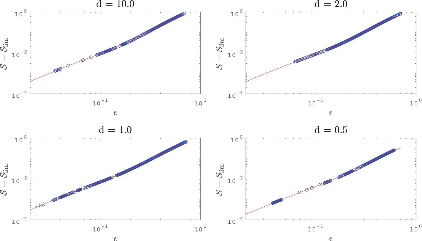
Figure 8. Fit of Longuet-Higgins and Fox’s steepness asymptotics (solid red line) to data (blue circles) in depths 10, 2, 1 and 0.5. These fits are more accurate when using a larger number of waves, as in depth 1. The data appears linearly dependent on epsilon with slope 2 for small values of the perturbation parameter $\epsilon$ on the log-log scale, indicating the validity of the asymptotics in finite depth.

Figure 9. Fit of Longuet-Higgins’ speed asymptotics (solid red line) to the data (blue circles) in depths 10, 2, 1 and 0.5. These fits, however good, lose accuracy at small values of steepness. They are more accurate when using a larger number of waves, as in depth 1.

Figure 10. Fit of Longuet-Higgins’ energy asymptotics (solid red line) to the data (blue circles) in depths 10, 2, 1 and 0.5. These fits, however good, lose accuracy at small values of steepness. They are more accurate when using a larger number of waves, as in depth 1.

Figure 11. Fit of Longuet-Higgins’ asymptotics (solid red line) to the zero Fourier mode of a wave profile $\hat{y}_0=\langle y\rangle$ (blue circles) in depths 10, 2, 1 and 0.5. These particular asymptotics have not been produced in infinite depth. The limiting value of $\langle y\rangle$ appears to decay proportional to $\tilde{\omega}(d)^{-2}$ in the same way as the limiting speed, steepness and energy are related to inverse powers of the modified dispersion relation.

Table 1. Limiting parameter values for various depths. Parentheses denote digits that change over a $95\%$ confidence interval provided using Matlab’s fit function. The last digit shown in the parentheses is the order of magnitude of the width of the confidence interval, so that $0.01903(41)$ represents that Matlab’s $95\%$ confidence is contained in the interval $(0.0190336,0.0190346)$. The first column shows the depth $D$. The second, fourth and fifth columns show the values of the steepness $\mathcal{S}_{\lim}$, speed $c_{\lim}$ and total energy $\mathcal{H}_{\lim}=T_{\lim}+P_{\lim}$ that the fit predicts for the steepest wave in each given depth. As Longuet-Higgins and Fox’s asymptotic forms are more accurate closer to the steepest wave, the third column provides an indication of the accuracy of these predictions

Table 2. Coefficients of the fits of Longuet-Higgins and Fox’s asymptotics in various depths. The last digit shown shows the width of the 95% confidence interval, and parentheses show the digits which change across this confidence interval

The change of these parameters, and in particular, the change of the properties of the limiting wave in shallow water, is also of interest. In Figure 12, we plot the change of these limiting quantities going from shallow water to deep water. In addition to being monotonically decreasing for decreasing depth, it is interesting that the change of each of these limiting values as a function of depth is well approximated by a power of a rescaled version of the modified dispersion relation $\tilde{\omega}(d)=\sqrt{\tilde{k}(d)\tanh(\tilde{k}(d)d)}$. In particular, the limiting speed appears to decay like $1/\tilde{\omega}$, the limiting steepness like $1/\tilde{\omega}^2$ and the limiting energy like $1/\tilde{\omega}^6$. As with the modified wave number $\tilde{k}$, these connections with the dispersion relation are not entirely surprising. In fact, since $\tanh(x)\to1$ as $x\to\infty$ and $\tilde{k}(d)\to\infty$ as $d\to 0$, $\tilde{\omega}(d)$ itself can be approximated well by $\sqrt{\tanh(d)}$, a branch of the dispersion relation with wavenumber 1, which leads to only a small increase in the relative errors of these fits. Furthermore, the steepness of the limiting wave $\mathcal{S}_{\lim}$ then decays proportional to $\omega^2(1,d)$, the speed $c_{\lim}$ of that wave proportional to $\omega(1,d)$ and the energy $\mathcal{H}_{\lim}$ proportional to $\omega^6(1,d).$ Although not shown in Figure 12, the limiting value of the zero mode of the surface elevation decays like $\omega^4(1,d)$. Figure 13 demonstrates that the other coefficients of Longuet-Higgins and Fox’s asymptotics decay like shifted scaled integer powers of $\omega(1,d)$ as well.

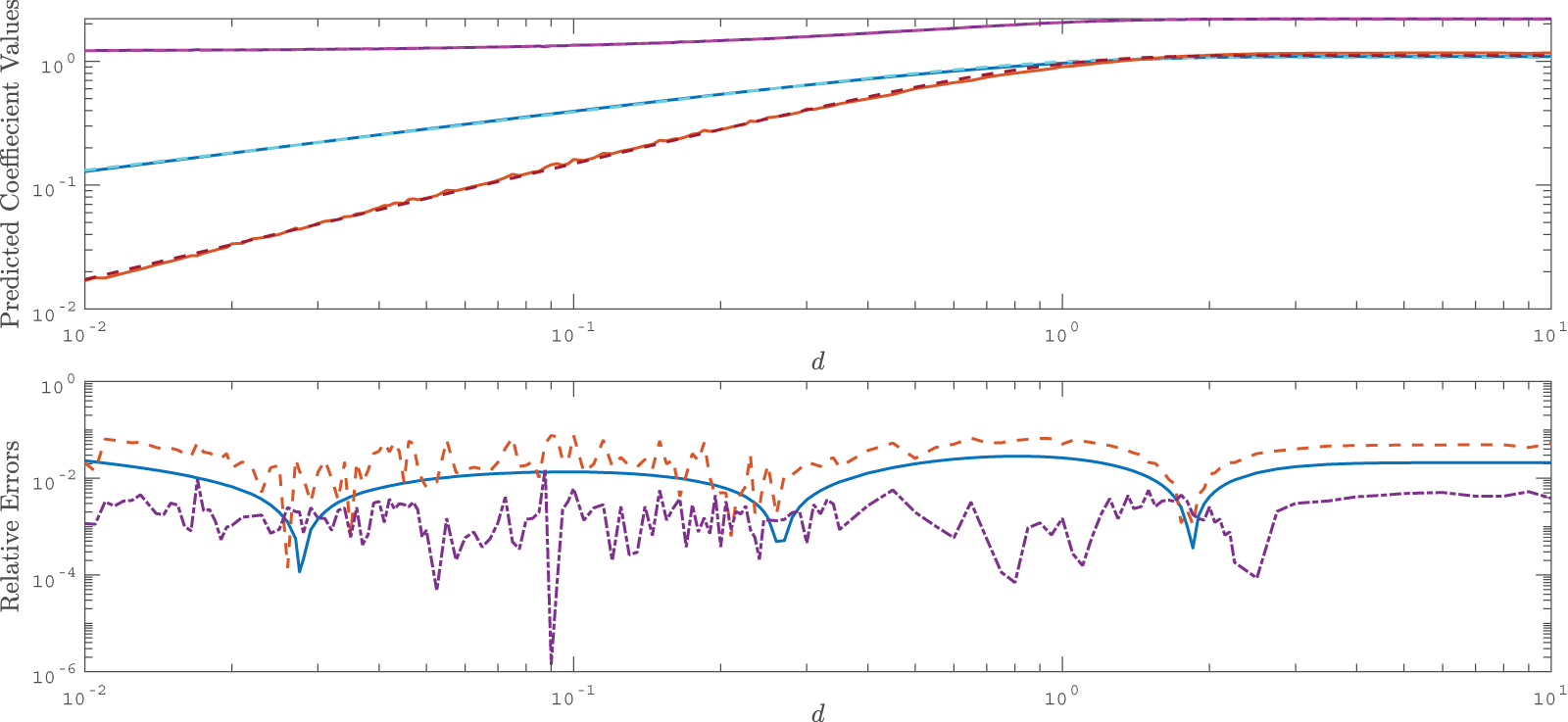
Figure 12. Top: Log-log plot of the predicted energy, speed and steepness of the limiting Stokes wave as a function of depth, as well as a number of fits to rescaled powers of the modified dispersion relation $\tilde{\omega}(d)=\omega(d,\tilde{k}(d))=\sqrt{g\tilde{k}(d)\tanh(\tilde{k}(d)d)}$. In particular, the speed is compared to $1.074\tilde{\omega}(0.81d)^{-0.479\cdot 2}$, the steepness to $0.886\tilde{\omega}(0.600d)^{-0.995\cdot 2}$ and the energy to $0.41\tilde{\omega}(0.77d)^{-2.9\cdot 2}.$ Data is shown in solid lines, the fit as dashed lines. The top lines (solid orange and dashed red) correspond to the speed of the limiting wave, the middle lines (solid blue and dashed cyan) correspond to the steepness of the limiting wave and the bottom pair of lines (solid purple and dashed magenta) correspond to the energy of the limiting wave. Bottom: relative errors between the fit and data. All errors are an order of magnitude smaller than the data. The errors appear structured, indicating that a power of the modified dispersion relation may be the first term in an asymptotic expansion involving these parameters. The solid blue line shows the relative residuals of the steepness fit, the dashed red line shows the relative residuals of the speed fit and the dashed-dotted purple line shows the relative residuals of the energy fit. Figure 13 shows the decay of other coefficients of (20).

Figure 13. Top: Log-log plot of the coefficients $c_{\lim}$ (blue), $-a_2$ (red) and $a_3$ (purple) of Longuet-Higgins and Fox’s speed asymptotics (20) as a function of depth, as well as a number of fits (dashed) to rescaled powers of the modified dispersion relation $\tilde{\omega}(d)=\omega(d,\tilde{k}(d))=\sqrt{g\tilde{k}(d)\tanh(\tilde{k}(d)d)}$, with a constant $1.20$ added into the fit of the phase shift $a_3$. In particular, the limiting speed fit is $1.074\tilde{\omega}(0.81d)^{-0.479\cdot 2}$, the $a_2$ fit is $1.1 \tilde{\omega}(0.8d)^{-0.95\cdot 2}$ and the $a_3$ fit is $1.19+1.0 \tilde{\omega}(0.8d)^{-0.91\cdot 2}$. Bottom: relative residuals for $c_{\lim}$ (solid blue), $a_2$ (dashed red) and $a_3$ (dash-dotted purple). All errors in the fits are all an order of magnitude less than the data and relatively structured (without the noise from our original fits), indicating this may be the first term in an asymptotic expansion of these coefficients. Similar fits hold for the coefficients of $T$, $U$, $\mathcal{S}$ and $\hat{y}_0=\langle y \rangle$.

Figure 14. Plot of the predicted steepness of the first few extremizers of the energy (solid blue) and speed (dashed red) relative to the predicted steepness of the steepest wave. Note that these extremizers interlace, as predicted in infinite depth.

4.2. Local extremizers of the speed and energy in varying depth

In Section 4.1, we used the computed Stokes waves to find asymptotic forms for the speed, steepness and energy as the limiting wave is approached in finite depth. We extract other information from these forms beyond these predicted limiting values. In particular, assuming that we can differentiate the asymptotic relations (20–23), we can approximate the steepness of each of the various extremizers of the speed and energy and the extreme values of these quantities by finding the extrema of their asymptotics.

To find the values of $\epsilon$ that extremize the asymptotic formula for speed, we solve

(29)\begin{equation} 0=\frac{dc_{LHF}^2}{d\epsilon}=\frac{g}{k}\left[3a_2\epsilon^2\cos(3\mu\ln(\epsilon)+a_4)+a_2\epsilon^3\sin(3\mu\ln(\epsilon)+a_4)\frac{3\mu}{\epsilon}\right], \end{equation}

where $c_{LHF}$ is the speed from the Longuet-Higgins and Fox asymptotic relations. Since the perturbation parameter $\epsilon$ and the steepness $\mathcal{S}$ are monotonically related, as shown in Figure 8, the extremizers of the speed as a function of steepness coincide with those of the speed as a function of amplitude. Recall that $a_2$ and $a_4$ are fit parameters from the asymptotic formula (20), and $\mu$ originates from the surface conditions and is a constant independent of depth. It follows that

(30)\begin{equation} \epsilon_k=\exp\left(\frac{\left(\pi k+\arctan\left(\frac{1}{\mu}\right)\right)-a_4}{3\mu}\right), \quad k\in \mathbb{Z}. \end{equation}

In (30), each integer $k$ corresponds to a distinct extremizer of the asymptotic formula (20). However, only for sufficiently small $k$ in (30) will $\epsilon$ correspond to values of (20) which approximate true extreme values of the speed. In particular, if we define $\epsilon_{c,n}$ to be the value of $\epsilon_k$ which approximates the perturbation parameter at the $n$th extremizer of the speed, we have that $n\to\infty$ as $k\to-\infty$. Regardless, it is interesting to note that (30) depends only on the phase-shift $a_4$, as $\mu$ is constant across all depths. As $c_{LHF}$ is positive for all $\epsilon$, it has the same extremizing $\epsilon$ as $c_{LHF}^2$.

Extremizing the energy is more complicated, as there are two terms. Using sine and cosine addition identities, we solve for the extremizing $\epsilon$. Using the coefficients listed in (21–22), the extremizers are

(31)\begin{equation} \epsilon_k = \exp\left(\frac{1}{3\mu}\left[k\pi+\arctan\left(-\frac{[b_2\cos(b_4)+\mu b_2\sin(b_4)+c_2\cos(c_4)+c_2\sin(c_4)]}{[b_2\mu\cos(b_4)-b_2\sin(b_4)+c_2\mu\cos(c_4)-c_2\sin(c_4)]}\right) \right]\right), \quad k\in \mathbb{Z}. \end{equation}

If the denominator of the argument of the arctan is zero, we choose the arctan term to be $\pi$. As in (30), $k$ parameterizes the different extremizers, with smaller $k$ corresponding to steeper extremizers of the energy. We define $\epsilon_{\mathcal{H},n}$ to be the value of $\epsilon_k$ which approximates the perturbation parameter at the $n$th extremizer of the energy. Since the speed at the crest varies from the phase speed at zero amplitude to 0 at the steepest wave, we are searching for $\epsilon$ in the range $[0,1/\sqrt{2}]$. We plot the change in the steepness of the first few extremizers of the energy and the speed in Figure 14, and list their steepness and values in Table 3. Despite their investigation of extreme waves and the limiting wave in various depths, Cokelet [Reference Cokelet4] and others [Reference Schwartz33, Reference Zhong and Liao44] did not discuss the local extremizers of these quantities. This is a notable gap in the literature considering the connections between these values and interesting points in the change of the topology of the stability spectra [Reference Dyachenko and Pelinovsky14, Reference Longuet-Higgins22, Reference Longuet-Higgins23, Reference Saffman32, Reference Tanaka38, Reference Tanaka39, Reference Zufiria and Saffman45].

Table 3. Predicted steepness of the first four extremizers of the speed and energy, and the corresponding values of speed and energy in a number of depths, computed using Longuet-Higgins and Fox’s asymptotics. Here $\mathring{\mathcal{S}}=2\pi \mathcal{S}$, to allow for direct comparison with the parameters of Longuet-Higgins and Fox

We check these results in different ways. Firstly, we compare with a direct computation of the steepness of the extremizers of the speed and energy. To do this, we find the solutions to (11) which extremize the speed or energy. This comparison is found in Table 4. In addition to knowing the steepness of the various extremizers of the energy and the speed, and how their values change as the limiting wave is approached, we consider a ratio of the steepnesses at which various extremizers occur. In particular, we define $S_{c,n}$, $S_{\mathcal{H},n}$ to be the steepness of the $n$th non-trivial extremizer of the speed and energy, respectively. We are interested in the limit as $n\rightarrow \infty$ of

Table 4. Comparison of various computed values of the steepness and energies of the first two non-trivial extremizers of the energy in depths 10, 1 and 0.1. The first set of three columns corresponds to the directly computed steepness of the first or second extremizer of the energy, the approximation of this steepness by the asymptotics of Longuet-Higgins and Fox, and the error between these values. Here $\mathring{\mathcal{S}}=2\pi \mathcal{S}$, to allow for direct comparison with the parameters of Longuet-Higgins and Fox

(32)\begin{equation} R_n = \frac{\mathcal{S}_{\mathcal{H},n}-\mathcal{S}_{c,n-1}}{\mathcal{S}_{c,n}-\mathcal{S}_{c,n-1}}. \end{equation}

The ratio $R_n$ measures how far between two extremizers of the speed the $n$th extremizer of the energy is located. To approximate this limit, we note that Longuet-Higgins and Fox’s perturbation parameter $\epsilon$ tends to zero as the steepest wave is approached. Thus, for large $n$, we approximate $R_n$ by

(33)\begin{equation} R_n\sim \frac{\mathcal{S}_{\lim}+d_1\epsilon_{H,n}^2-(\mathcal{S}_{\lim}+d_1\epsilon_{c,n-1}^2)}{\mathcal{S}_{\lim}+d_1\epsilon_{c,n}^2-(\mathcal{S}_{\lim}+d_1\epsilon_{c,n-1}^2)}=\frac{\epsilon_{H,n}^2-\epsilon_{c,n-1}^2}{\epsilon_{c,n}^2-\epsilon_{c,n-1}^2}. \end{equation}

Using (30) and (31),

(34)\begin{equation} \epsilon_{c,n} = \epsilon_{c,n-1}e^{-\frac{\pi}{3\mu}},\quad\text{and}\quad \epsilon_{\mathcal{H},n} = \epsilon_{\mathcal{H},n-1}e^{-\frac{\pi}{3\mu}}. \end{equation}

To justify (34), note that as $n\to \infty,$ $k \to -\infty$ in (30) and (31) and $\epsilon \to 0$ so the steepest wave is approached. We see that

(35)\begin{align}\lim_{n\to\infty} R_n &\sim \lim_{n\to\infty} \frac{\epsilon_{\mathcal{H},n}^2-\epsilon_{c,n-1}^2}{\epsilon_{c,n}^2-\epsilon_{c,n-1}^2}\nonumber \\ &=\frac{e^{-\frac{2\pi}{3\mu}(n-2)}\left(\epsilon_{\mathcal{H},2}^2-\epsilon_{c,1}^2\right)}{e^{-\frac{2\pi}{3\mu}(n-2)}\left(\epsilon_{c,2}^2-\epsilon_{c,1}^2\right)}\nonumber\\ &=\frac{e^{-\frac{2\pi}{3\mu}}\epsilon_{\mathcal{H},1}^2-\epsilon_{c,1}^2}{\epsilon_{c,1}^2\left(e^{-\frac{2\pi}{3\mu}(n-2)}-1\right)}\nonumber\\ &=\frac{e^{-\frac{2\pi}{3\mu}}\frac{\epsilon_{\mathcal{H},1}^2}{\epsilon_{c,1}^2}-1}{e^{-\frac{2\pi}{3\mu}}-1}.\end{align}

Thus, we compute the limiting ratio using just the ratio of the perturbation parameters corresponding to the first extremizers of the energy and speed. We could have used steeper extremizers as well, but the first one is most accessible. We compute this limiting ratio in different depths and present the results in Figure 15. Despite the noise introduced by the Longuet-Higgins and Fox asymptotics in a regime far beyond their validity, we can fit a rescaled, shifted power of the dispersion relation $\omega^2 = gk\tanh(kd)$ to this data, with an exponent whose confidence interval includes 1.

Figure 15. Fit of the value of the approximation to the limit $\lim_{n\to\infty}R_n$, see (32), as a function of depth to a rescaled shift of an inverse power of the modified dispersion relation $\tilde{\omega}(d)$. The relative error of the fit is on the order of $10^{-3}$ when we set the inverse power to $-1$. Computing these ratios with more waves may reduce the noise in our data and allow for more accuracy and confidence in this fit. The solid blue line is the computed value of the limiting ratios, whereas the dashed red line is a fit $0.98-0.3\tilde{\omega}(0.9d)^{-1}.$.

5. Branch point singularities

We study the singularity structure of the analytic continuation of the Stokes waves and compare it to that of infinite depth waves [Reference Crew and Trinh6, Reference Dyachenko, Lushnikov and Korotkevich12, Reference Dyachenko, Lushnikov and Korotkevich13, Reference Grant17, Reference Longuet-Higgins and Fox24, Reference Lushnikov27, Reference Schwartz33]. To our knowledge, most of these works have not been extended to finite depth. In infinite depth, knowledge of the singularities has not only been used to better understand the formation of a $120^\circ$ corner but also to develop more efficient methods to compute and study these waves. Similarly, it is of great interest to understand the singularity structure in finite depth. In particular, our goal is to generalize the results of Dyachenko et al. [Reference Dyachenko, Lushnikov and Korotkevich12] to the finite-depth case.

Using conformal variables, Dyachenko et al. [Reference Dyachenko, Lushnikov and Korotkevich12] deform the contour of integration in the integral definition of the Fourier coefficient to encircle the singularity above the fluid. The decay of these coefficients directly relates to the type of singularity above the fluid. In particular, if the singularity has a dominant contribution

(36)\begin{equation} z \sim c_1(w-iv_c)^{\beta}, \end{equation}

then the Fourier spectrum of $z$ decays as

(37)\begin{equation} |z_k| \sim |k|^{-1-\beta}\exp(-|k|v_c),\quad k \to -\infty. \end{equation}

Dyachenko et al. [Reference Dyachenko, Lushnikov and Korotkevich12] found a square root-type branch point above the fluid, and determined that $v_c$ decayed as

(38)\begin{equation} v_c\sim \left( \mathcal{S}_{\lim}-\mathcal{S} \right)^{\delta}, \end{equation}

where $\delta = 1.48 \pm 0.03$ includes $3/2$ within its confidence interval.

A natural change from infinite depth comes from the presence of singularities beneath the conformal domain. Recall that the velocity potential $\phi$ satisfies the Laplace equation (1) within the bulk of the fluid with a Neumann boundary condition (2) on the bottom boundary. Thus, the analytic continuation of solutions beneath this boundary satisfies a mirror principle. In conformal variables, $\phi(u,v)=\phi(u,-2h-v)$. Thus any singularity above the conformal domain is mirrored beneath the conformal domain, as shown in Figure 16.

Figure 16. Waves of increasing steepness in depth 1, and the conformal mapping. Coloured dots correspond to coloured waves, showing the approach of singularities above and below the fluid to the conformal domain. The vertical axis for the right figure displays $x/h$, to account for different conformal depths for steeper waves in constant physical depth.

To leading order, a singularity beneath the fluid has the form

(39)\begin{equation} z = c_2(w+iv_c')^{\beta'},\quad v_c' \gt 2h. \end{equation}

If we deform the contour of the integral

(40)\begin{equation} z_k = \frac{1}{2\pi}\int_{-\pi}^\pi z(u)e^{iku}du,\quad k \gt 0, \end{equation}

around a singularity below the fluid, we find the asymptotic form

(41)\begin{equation} |z_k| \sim |k|^{-1-\beta}\exp(-|k|v_c'),\quad k \to \infty. \end{equation}

To determine $v_c'$ and $\beta'$ for the singularity beneath the fluid, we use Stokes waves computed with 64 bits of precision and fit the Fourier spectrum to (37–41) using Julia’s non-linear fitting routine, with accuracy $10^{-32}$. For every wave, it is confirmed that the locations of the singularities above and below the fluid are directly linked through the conformal depth $h$, with the quantity $v_c'+v_c+2h$ on the order of $10^{-3}$ or less for every wave checked. A sample fit of the decay of the spectrum of a relatively steep wave in depth 0.2 is shown in Figure 17. Since $\beta = \beta'=1/2$, these fits show that there are square-root type branch points both above and below the conformal domain. This verifies the predictions of Grant [Reference Grant17] and Tanveer [Reference Tanveer40] about the singularity above the fluid, as well as the use of the mirror principle to understand the singularity below the fluid for finite-depth Stokes waves.

We repeat the calculations of Dyachenko et al. [Reference Dyachenko, Lushnikov and Korotkevich12] regarding the branch point above the fluid domain of various extreme waves in double precision. Figure 18 demonstrates that the singularity above the fluid in depth 0.01 approaches the conformal domain in the same manner as described by Dyachenko et al. [Reference Dyachenko, Lushnikov and Korotkevich12, Reference Dyachenko, Lushnikov and Korotkevich13] and Lushnikov [Reference Lushnikov27]. In Figure 19, we show that this rate of approach is effectively constant as a function of depth. The similarity of these results is encouraging for an exploration of the structure of the Riemann sheet connected to this branch point [Reference Crew and Trinh6, Reference Lushnikov27], or the development of more efficient methods for the computation of waves in a fixed finite depth [Reference Dyachenko, Hur and Silantyev11, Reference Lushnikov, Dyachenko and Silantyev26, Reference Tanveer40]. Further investigations of the behaviour of these branch points in the shallow water regime are left for future work.

Figure 17. Top: Fit of the asymptotics given in (37) and (41). Bottom: relative residuals on a semi-log scale. Note the high degree of accuracy for $k$ sufficiently far from zero. A portion of the relative error between the positive Fourier coefficients and the fit is cut off, as the coefficients are at the level of noise, leading to growing relative errors in this regime despite a good fit. The solid blue line shows the Fourier modes of the surface elevation $y$ and the dashed red line shows the fits.

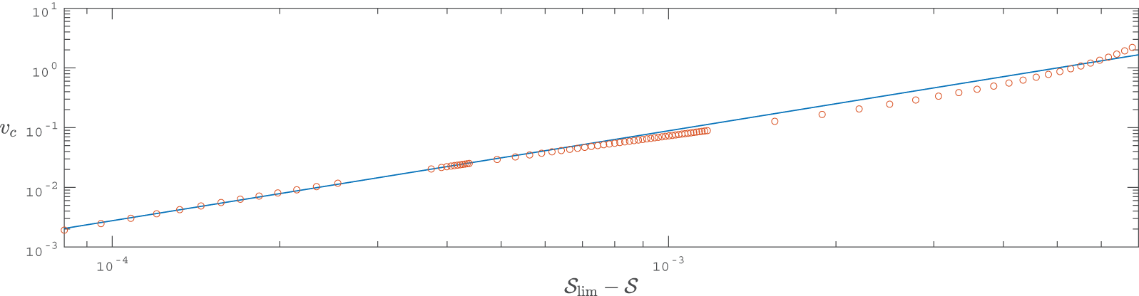
Figure 18. Fit of singularity location above the fluid $v_c$ as a power of the difference in steepnesses $\mathcal{S}_{\lim}-\mathcal{S}$ in depth 0.01. In this shallow water, as in infinite depth, a rate of decay of approximately 1.5 is predicted. The relative residual of the error between our fit and the data is bounded by $10^{-1}$ for extreme waves, suggesting this is a first-order term. The red circles are the computed branch point locations, and the blue line is a fit.

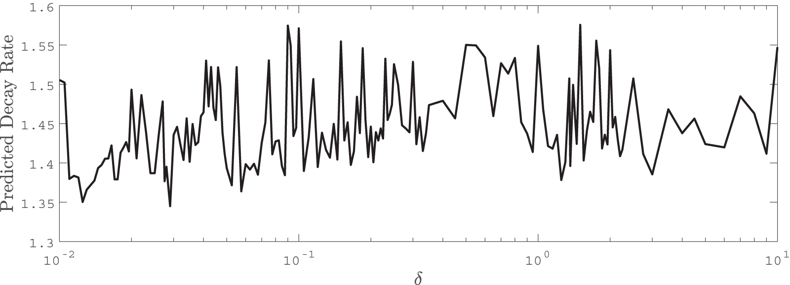
Figure 19. Change in the exponent $\delta$ of (38), the location of the singularity above the fluid as depth varies. Note that all predicted exponents are close to 1.5, as in infinite depth. Noise is largely due to which depths have more or fewer computed waves.

6. Conclusion

The method of Semenova et al. [Reference Semenova and Byrnes34] is modified to compute high-amplitude Stokes waves in a fixed physical depth. We also performed direct comparisons with the asymptotic analysis of Longuet-Higgins and Fox [Reference Longuet-Higgins and Fox24, Reference Longuet-Higgins and Fox25], fitting the coefficients of their asymptotics to numerical data to see how their approximations change as water depth is decreased. The leading coefficients of the approximations (31) and (30) are related to various integral qualities of the limiting wave, which we fit to half-integer powers of a modified dispersion relation as a function of depth. This modification accounts for the increasing localization of steep Stokes waves as depth decreases. Further, we fit the coefficients of higher-order terms to this dispersion relation. These asymptotic forms are used to predict the amplitudes at which the speed and energy are locally extremized.

The singularity structure of Stokes waves in finite depth is also studied. Similar to infinite depth, we found that Stokes waves have a square-root type singularity above the conformal domain, which approaches the free surface at a rate relatively insensitive to depth. In particular, the singularity appears to be found at $(\mathcal{S}_{\lim}-\mathcal{S})^\delta$, where $\delta$ is about 1.5 in each depth. We demonstrate the existence of a mirrored branch point of the same order beneath the conformal domain, whose location is reflected across the bottom of the fluid domain due to the Neumann condition there. We believe that it is the linear approach of this singularity to the domain as a function of depth and its cancellation with the singularity above the surface, which leads to the near localization of the Stokes wave in shallow water.