

1. Introduction
We inquire why a parent might use or refrain from using child labor. What we find is based on a parent's demand for gratitude from his child, which we model as an intervening variable between the parent's earnings and the incidence of child labor.
The prevalence of child labor in the agricultural sector of developing countries is a matter of concern. Data are not precise, but the general picture is clear: around 70 percent of child labor in the world occurs in the agricultural sector (ILO, 2017), with most of it happening in developing countries (FAO, 2020).Footnote 1 One implication of these raw data is that agricultural development policies ought to prioritize programs aimed at influencing the use of child labor in agriculture. For example, obtaining higher crop yields per acre without reducing the use of child labor does not amount to modernization of agricultural production. Therefore, understanding the incidence of child labor should matter to students of agricultural development.
The choice of what to grow on a family farm is linked with the use of child labor. Children are particularly good at some tasks such as picking cotton (Kazianga and Makamu, Reference Kazianga and Makamu2017). The possibility that the demand for gratitude will act to restrain the use of child labor and thereby lower the appeal of, for example, cotton production is intriguing.
Agricultural development policies include policies aimed at influencing the incidence of the use of child labor in agriculture. For example, there are frequent proposals to introduce pension or social protection schemes in developing countries. To better predict the consequences of such policies, it is essential to understand the mechanisms that give rise to child labor, and their links with factors such as parental income and parental demand for gratitude from children. As implied by our modeling below, an unintended consequence of the schemes could be a reduced demand for gratitude from children and, consequently, increased use of child labor.
In this paper we link the incidence of child labor with the parent's demand for gratitude, and we connect variation in the level of this demand with variation in the parent's earnings. Recalling the concept of gratitude formation (Stark and Falk, Reference Stark and Falk1998) where transfers to others are governed by a desire to elicit gratitude, we conjecture that the parent's demand for gratitude can act as a check on child labor. In the “production function” of gratitude, refraining from using child labor is an input. The demand for gratitude arises from the desire of the parent to receive care and support when the parent reaches old age, and the child has become an adult who is plausibly capable, but not necessarily willing, to provide support. Needless to add, support from an adult child is particularly needed when official old age support is not available. A sense of gratitude connects the will to deliver care with the ability to supply care. One difference between this perspective and existing models of child labor (among others, Basu and Van, Reference Basu and Van1998; Baland and Robinson, Reference Baland and Robinson2000; Ravallion and Wodon, Reference Ravallion and Wodon2000; Bhalotra, Reference Bhalotra2007; Basu et al., Reference Basu, Das and Dutta2010) is that the emphasis here is not on how current consumption needs lead to child labor but, rather, on how the need for future care and support leads to withdrawal of child labor.
Because we believe that parental altruism towards the child is not a function of the parent's earnings, our proposed explanation for the variation in the incidence of child labor is not based on variation in parental altruism.
In terms of their earnings, we consider parents of three types: very poor, not-so-poor, and fairly rich. A very poor parent would like to instill gratitude, but he cannot afford to; his current needs crowd out his future needs, so he resorts to child labor. A not-so-poor parent would like to instill gratitude and can afford to do that, so he does not resort to child labor. A fairly rich parent may not require gratitude; upon reaching old age he will have the means to support himself, so a restraint on child labor arising from a demand for gratitude may not apply. In addition, if there is much to tend to in a relatively large plot, the child's work will be needed, especially when hired labor is hard to get and / or hard to manage; child labor could be a result. Thus, the picture looks as follows.
Parent: very poor not-so-poor fairly rich
Demand for gratitude: yes yes no
Child labor: yes no possibly yes, possibly no
Therefore, it is possible that with respect to the parent's earnings we will observe a U-shaped pattern of child labor.
2. A modeling framework
We assume that the parent lives for two periods.
The parent's first period utility function is
 $$U_1( s, \;h) = \log ( w_a + w_ch-s) , \;$$
where w a > 0 is the parent's wage (a for adult), w c > 0 is the child's wage (c for child). We assume that w a > w c. The wages referred to in our model are imputed wages, meaning measures of the evaluation of the returns from labor, or shadow wages, meaning wages that can be earned in alternative but similar employment / the equivalents of wages that individuals would receive if they were to “rent out” their labor. Obviously, and for example, when dealing with a child who works on the farm of his parent, the child is not normally paid a wage, so the clarification made here needs to be borne in mind. The parent can choose the amount of savings, s, out of the combined (parent and child) first period wages, as well as the intensity of the child's labor, 0 ≤ h ≤ 1. When h = 0 the child does not work and, thus, does not contribute to the household income; when h = 1 the child works the maximal number of hours possible (normalized at one), contributing w c to the household income.
The parent's second period utility function is
 $$U_2( s\hskip.2pt, \;s_c) = \log ( s + s_c) , \;$$
where s c denotes the support received from the child when the child is an adult and the parent is in the second period of his life. In the second period of the parent's life, the child, who by then is an adult, is assumed to maximize the utility function
 $$U_c( s_c\hskip.2pt, \;h) = \log ( w_a-s_c) + ( 1-h) \log ( s_c) . $$
To enable us to concentrate on essentials, we assume that on becoming an adult, the child earns the same wage w a as the parent did in the earlier period. This assumption also helps to separate low intensity of child labor from schooling, which in this paper we do not assume to be the same thing (consult Section 3 for a discussion of this issue). If child labor were an alternative to schooling, then it could be the case that the child's wage during his adulthood will depend inversely on h, namely that a lower intensity of child labor could entail more schooling which could lead to a higher wage upon becoming an adult. But this is not the case here. The term (1 − h) represents the gratitude of the child towards the parent, taken to be a function of the intensity of the child's labor during childhood: it is a measure of the value accorded by the child to providing support for the parent, incorporating the idea that the lighter the work burden during childhood, the greater the gratitude. The extent of this valuation is “engineered” by the parent when he chooses the level of h in the first period of his life.
From (3) it follows that (i): if h = 1, then the child's utility is maximized by setting s c = 0: when the child's labor is at its maximal intensity, the child provides no support to the parent in the parent's second period of life. And (ii): if h = 0, then the child's utility is maximized by setting  $s_c = {{w_a} \over 2}.$ To find out the child's optimal level of support for any chosen level of h, we differentiate U c(s c, h) in (3) with respect to s c. This yields the first order condition
 $$-\displaystyle{1 \over {w_a-s_c}} + \displaystyle{{1-h} \over {s_c}} = 0.$$
From (4) it follows that for any chosen level of h ∈ [0, 1], the child (as an adult) maximizes his utility function by choosing the level of support
 $$s_c( h) = \displaystyle{{w_a( {1-h} ) } \over {2-h}}.$$
Footnote 2In expressing s c as s c(h), we consider it as a function of h, defined by equation (4’). We note that the function s c(h) satisfies properties that we would expect from a function of the level of support motivated by gratitude. In particular,  ${{\partial s_c( h) } \over {\partial h}} < 0$, namely the level of support provided by the child when he is an adult depends negatively on the intensity or the amount of labor that he was made to supply when he was a child.
Comment. Qualitatively, the results reported above are not conditional on a logarithmic representation of the utility functions, although and obviously, qualitatively they will differ under an alternative representation. An example of an alternative representation of the equation in (3) is
 $$U_c( s_c, \;h) = f( w_a-s_c) + ( 1-h) g( s_c)$$
where f(⋅) and g(⋅) are increasing, concave, and twice differentiable. For (3’), the property referred to following (4’), namely the property  ${{\partial s_c( h) } \over {\partial h}} < 0$, applies. To see this we note that the first order condition with respect to s c takes the form:
 $$-{\,f}^{\prime}( w_a-s_c) + ( 1-h) {g}^{\prime}( s_c) = 0.$$
Applying the implicit function theorem to F(s c, h) = −f′(w a − s c) + (1 − h)g′(s c) = 0, we obtain
 $$\displaystyle{{\partial s_c( h) } \over {\partial h}} = \displaystyle{{{g}^{\prime}( s_c) } \over {{\,f}^{\prime \prime}( w_a-s_c) + ( 1-h) {g}^{\prime \prime}( s_c) }} < 0, \;$$
where  ${{\partial s_c( h) } \over {\partial h}} < 0$ holds because g′(s c) > 0, f″(w a − s c) < 0, and g″(s c) < 0.
We naturally assume that the parent maximizes his two-period utility function. Using (1), (2), and (4’), this utility function is
 $$U( s\hskip.2pt, \;h) = U_1( s\hskip.2pt, \;h) + \rho U_2( s\hskip.2pt, \;h) = \log ( w_a + w_ch-s) + \rho \log \left({s + \displaystyle{{w_a( {1-h} ) } \over {2-h}}} \right), \;$$
where ρ ∈ (0, 1) is the intertemporal discount factor. The first order conditions obtained from calculating  ${{\partial U( s\hskip.2pt, \;h) } \over {\partial s}}$ and ${{\partial U( s\hskip.2pt, \;h) } \over {\partial h}}$ are given, respectively, by
 $${\vskip22pt{\hscale100%\vscale1000%{\{}}}\left.{\matrix{ {-\displaystyle{1 \over {w_a + w_ch-s}} + \displaystyle{\rho \over {s + \displaystyle{{w_a( {1-h} ) } \over {2-h}}}} = 0} \cr {\displaystyle{{w_c} \over {w_a + w_ch-s}}-\displaystyle{{\rho \displaystyle{{w_a} \over {{( {2-h} ) }^2}}} \over {s + \displaystyle{{w_a( {1-h} ) } \over {2-h}}}} = 0, \;} \cr } } \right.}$$
which, upon rearrangement, yield the set of equations
 $${\vskip12pt{\hscale100%\vscale550%{\{}}}\left.{\matrix{ {\rho ( w_a + w_ch-s) = s + \displaystyle{{w_a( {1-h} ) } \over {2-h}}} \cr\cr { w_c\left({s + \displaystyle{{w_a( {1-h} ) } \over {2-h}}} \right) = \rho \displaystyle{{w_a} \over {{( {2-h} ) }^2}}( w_a + w_ch-s) .} \cr } } \right.}$$
On substituting the first equation in (7) into the second equation in (7) we get
 $$w_c\rho ( w_a + w_ch-s) = \rho \displaystyle{{w_a} \over {{( {2-h} ) }^2}}( w_a + w_ch-s) , \;$$
which simplifies to
 $$w_c = \displaystyle{{w_a} \over {{( {2-h} ) }^2}}.$$
From (9) it follows thatFootnote 3
 $$h = {\vskip12pt{\hscale100%\vscale550%{\{}}}\left.\matrix{2-\sqrt {\displaystyle{{w_a} \over {w_c}}} \qquad{\rm if\ }\displaystyle{{w_a} \over {w_c}} < 4 \hfill \cr\cr 0\qquad\vskip0.6pc\hskip2.6pc{\rm if\ }\displaystyle{{w_a} \over {w_c}} \ge 4. \hfill} \right.}$$
It is intuitive that when in comparison with the parent's wage the child's wage is pretty low (that is, as per the second part of (10), when  $w_c \le {{w_a} \over 4}$) the maximal utility is obtained at the corner solution h = 0: when a child's wage is quite low, it is more beneficial for the parent to wait for support to be provided in the second period rather than let the child work in the first period for a relatively small supplementary income.
Looking at (10), we see that for a given w c, the intensity of child labor decreases with the parent's wage, w a. As noted below, this result aligns with a result reported in part of the existing literature. However, if w c is a function of w a (a discussion of this possibility is in the next paragraph), then the outcome can differ. When we so assume, we can denote the intensity of child labor as a function of the parent's wage, h(w a), namely
 $$h( w_a) = 2-\sqrt {\displaystyle{{w_a} \over {w_c( w_a) }}} .$$
In this case,
 $$\displaystyle{{\partial h( w_a) } \over {\partial w_a}} = {-}\displaystyle{1 \over 2}\sqrt {\displaystyle{{w_c( w_a) } \over {w_a}}} \displaystyle{{w_c( w_a) -\displaystyle{{\partial w_c( w_a) } \over {\partial w_a}}w_a} \over {w_c{( w_a) }^2}}.$$
From (11) it follows that  ${{\partial h( w_a) } \over {\partial w_a}} > 0$ will hold only if $w_c( w_a) -{{\partial w_c( w_a) } \over {\partial w_a}}w_a < 0$. This inequality can be rewritten as
 $$\displaystyle{{\partial w_c( w_a) } \over {\partial w_a}}\displaystyle{{w_a} \over {w_c( w_a) }} > 1.$$
The inequality in (12) informs us that if the elasticity of the child's wage with respect to the parent's wage is higher than 1, then  ${{\partial h( w_a) } \over {\partial w_a}} > 0$: the intensity of child labor will increase with an increase in the parent's wage. Why?
To see how in the wake of an increase in the parent's wage child labor will be intensified, suppose that an agricultural activity for which a parent receives a wage, say growing a particular crop, increases in value (the demand for the crop increases markedly) and that, consequently, deliveries of the produce to the market become more valuable. With both the reward of growing the crop and the attractiveness of more frequent deliveries to meet the higher market demand becoming higher, we will observe that the wage of the parent and the intensity of the child's labor, whose job it is to make the deliveries, will increase in parallel.
Another possible reason could relate to nutrition and health, spheres where the child is highly vulnerable, and more so than an adult. An increase in the parent's wage translating into better nutrition for the household will have a clearly positive effect on the productivity (productive capability) of the child and, consequently, on the child's wage. Admittedly, this reasoning does not substitute for direct evidence in support of condition (12). However, our search for such evidence was unsuccessful. Nor could we find evidence to the contrary. It appears that the elasticity of the child's wage with respect to the parent's wage was not investigated. Bearing this in mind, we review two cases.
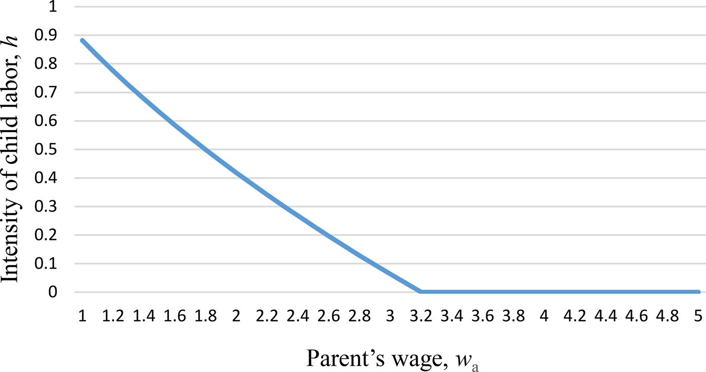
First, in Figure 1 we present a case in which the child's wage is a constant; for example, we set w c(w a) = 0.8. In this case,  ${{\partial w_c( w_a) } \over {\partial w_a}} = 0$, so condition (12) is clearly not satisfied and, therefore, we observe a non-increasing relationship between the intensity of child labor and the parent's wage: for a poor parent we observe a high intensity of child labor; for a not-so-poor parent we observe a low intensity of child labor or no child labor; and for a fairly rich parent we observe no child labor.
The intensity of child labor as a function of the parent's wage: The example of w c(w a) = 0.8. The function used to plot the curve in this Figure is  $h( w_a) = \max \left({2-\displaystyle\sqrt {{{w_a} \over {0.8}}}\, , \;0} \right)$. For w a ≥ 3.2, the value of this function is 0.
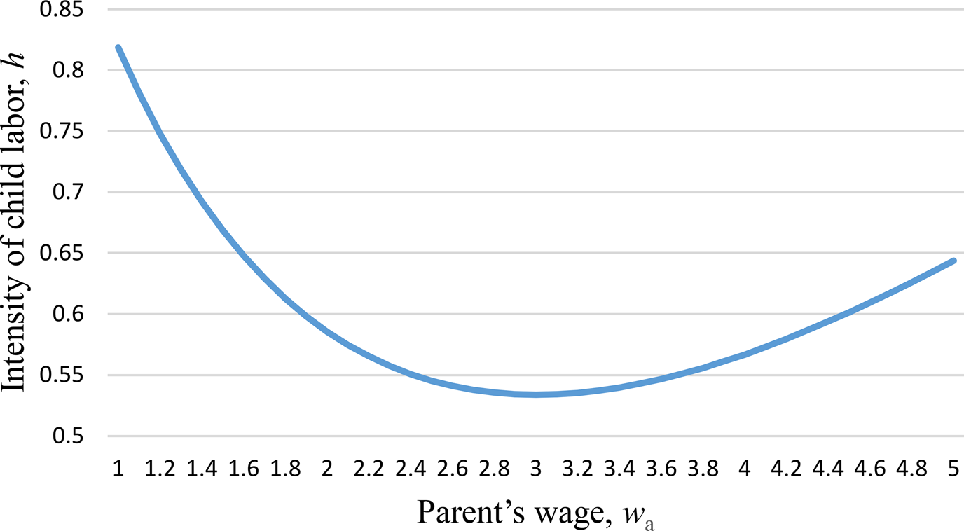
Second, our proposed formulation can yield a U-shaped pattern of the relationship between the intensity of child labor and the parent's wage. To see this, we allow the child's wage to depend on the parent's wage, for example by letting  $w_c( w_a) = e^{{{w_a-2} \over 3}}$.Footnote 4 Then, condition (12), that now takes the form ${{e^{{{w_a-2} \over 3}}} \over 3}{{w_a} \over {e^{{{w_a-2} \over 3}}}} = {{w_a} \over 3} > 1$, is satisfied for w a > 3. Consequently, as depicted in Figure 2, over the same domain as that of Figure 1, the relationship between the intensity of child labor and the parent's wage is U-shaped.
The intensity of child labor as a function of the parent's wage: The case of  $w_c( w_a) = e^{{{w_a-2} \over 3}}$. The function used to plot the curve in this Figure is $h( w_a) = 2-\sqrt {{{w_a} \over {e^{{{w_a-2} \over 3}}}}} $. At w a = 3, the function has an inflection point.
3. Discussion
An interesting implication of the preceding line of reasoning is that the incidence of the “wealth paradox” of child labor, namely that, as documented for example in the case of rural households in Pakistan and Ghana, the children of land-rich parents work more than the children of land-poor parents (Bhalotra and Heady, Reference Bhalotra and Heady2003), could be partially explained, or further supported, by the absence of a check on child labor that arises from a desire to “acquire” gratitude.Footnote 5
Another interesting implication is that an increase in income (wages) will not in and of itself be a “cure” to the problem of child labor if, over some range, rising income weakens the gratitude-based incentive of parents to refrain from making children work; the notion that higher income will automatically and consistently eradicate child labor may not be correct. Illuminating supportive evidence in this regard is provided by Chong and Yáñez-Pagans (Reference Chong and Yáñez-Pagans2019). In their study of rural Bolivia, they identify a positive effect of the national unconditional cash transfer program on the intensity of labor by boys. Chong and Yáñez-Pagans write (p. 60): “[R]ural households tend to invest the proceeds of unconditional transfers, which then translates in increases in output. … The unconditional transfer may create incentives for child labor participation in rural settings by increasing the boys’ relative productivity in the labor market and therefore by increasing the opportunity cost of leisure and schooling for boys in rural areas.” Similar effects are reported by Kruger (Reference Kruger2007) who provides evidence that in Brazilian coffee regions improved incomes were associated with higher child work, and by de Carvalho Filho (Reference Filho and Evangelista2012) who finds that in rural Brazil increased income did not lead to a decrease in child labor. Studying a cash transfer program in yet another Latin American country, Edmonds and Schady (Reference Edmonds and Schady2012) find that in Ecuador, the transfer delays sending school children to work, whereas it has no effect on children who are already working.
Our explanation for the change in the incidence of child labor as a function of parents’ earnings is different from the explanation provided by Basu and Van (Reference Basu and Van1998), who draw on a “luxury axiom” which states that the poorest households cannot afford the “luxury” of child school attendance, while richer households can, and do, refrain from sending their children to work. We differ in that our prediction is that “richer people” who are less poor behave differently from “richer people” who are fairly rich. Ray (Reference Ray2000) does not find support for the “luxury axiom” in Peru and Pakistan.
Our approach resembles the approach of Becker et al. (Reference Becker, Murphy and Spenkuch2016), who presume that by spending resources, a parent can mold the future preferences of a child (such as the child's altruism towards him). Similarly, we postulate that in order to affect a child's preferences (here, to instill in the child a sense of gratitude), a parent forgoes increased income from child labor. However, in several respects we differ from Becker et al. in that we do not base our reasoning on an assumption that the parent is altruistic towards his child, and in that the focus of our analysis is on the link between the incidence of child labor and the earnings of the parent.
The idea that the demand for gratitude restrains child labor places a new “substitution” at center stage: the substitution that is at the core of the “luxury axiom,” namely that child labor and adult labor substitute for each other, is replaced by the perspective that child labor and gratitude formation are substitutes.
Our perspective differs from a perspective based on human capital formation (investment in schooling). Although children's acquisition of human capital could enable them - through higher earnings - to provide support to their parents, ability is not the same as willingness. Gratitude is the bond, and gratitude could emanate from being allowed to attend school rather than being sent to work. Suppose that the large majority of children in village A go to school. A child in a family in village A who is sent to school will not be particularly grateful; schooling is natural. Suppose that the large majority of children in an otherwise similar village B do not go to school but work. A child in a family in village B who is sent to school will be grateful for not being sent to work. Schooling is exceptional. Thus, schooling alone will not suffice to produce gratitude, which is a critical catalyst in transforming returns from human capital formation into transfers to elderly parents. The intensity of a child's gratitude could also be influenced by the use of child labor in generations of the child's family. If a child's parent and the parent's parent were sent to work during their childhood but the current generation's child is not sent to work, then other things being the same, the child's appreciation of not being sent to work will be greater than if in past generations children were not sent to work. A deviation from tradition will be appreciated by more than adherence to tradition.
The distinction between our perspective and that of human capital needs to be sharp: throughout this paper, the opposite of child labor is not schooling. A straightforward way to drive home this point is that as in set theory, the opposite of child labor are the “elements” not in “child labor.” These elements can include schooling, but need not; play, socializing with other children, and letting the child choose between these and other activities are “elements” too. Moreover, to think that schooling and child labor are mutually exclusive (substitutes) may be conceptually wrong when, for example, after school hours, a child is ordered by the parent to do farm work.
Our perspective also differs from a perspective alluded to in writings on gratitude formation and intergenerational transfers (for example, Stark, Reference Stark1999, and Cox and Stark, Reference Cox and Stark2005). Refer to a child as K, to a parent as P, and to an elder as G. The literature on intergenerational transfers as an expression of gratitude considers the time of gratitude formation to be the period during which P provides G with attention and care, with bequests from G to P constituting a reward. The time span in which gratitude is created is, so to speak, the P-G span. A novelty of this paper is to roll back in time the period of gratitude formation; it is, so to speak, the K-P time span: the seeds of future provision of attention and care are sowed when and as P frees K from work, with attention and care provided by K to P when K becomes a P, and P becomes a G. Thus, the timing and the mechanism that instill gratitude studied in this paper differ from the one studied in the existing literature on how gratitude is “produced,” and how it is rewarded.
Because our focus is on child labor, the main variable that is of interest to us is the intensity of child labor, h. Nonetheless, our model also yields a prediction for the other decision variable of the parent, namely with regard to the saving rate, s. Specifically, our model implies that a higher wage of the child drives up the parent's savings:  ${{\partial s} \over {\partial w_c}} \ge 0$.Footnote 6 Intuitively, a higher child's wage renders child labor more attractive, which in turn causes the child's gratitude to be lower. The mechanism at work is that, as per (10), when the wage of the child increases, child labor increases; and a higher intensity of child labor entails lower gratitude. In face of diminished gratitude, the parent will need to rely more on savings to support himself in old age.
The model presented in this paper abstracts from fertility decisions; we referred to a child, not to children. It could be argued that if it is important to parents to have a grateful child, and if there is uncertainty in that regard, then a parent may want to have several children so that in due course at least one of them will transform gratitude into support. There is extensive analysis of the idea that in poor countries children as adults are a source of old age support, akin to pensions in rich countries, so dwelling on this perspective is not required here. What could, however, be intriguing and novel is to develop a model of the demand for children and variation in that demand, not as consequences of the demand for support in old age per se but, rather, as consequences of the demand for gratitude. Our framework both provides a starting point and suggests alternative parental strategies: greater effort to “inculcate” into a given child a deeper sense of gratitude as opposed to inculcating moderate levels of gratitude into several children.


 Open access