

Introduction
Synthetic Aperture Radar (SAR) data has been widely used to determine flow velocities and stress/strain fields for understanding the dynamics of fast flowing Greenlandic outlet glaciers (Joughin and others, Reference Joughin, Kwok and Fahnestock1996; Strozzi and others, Reference Strozzi, Luckman, Murray, Wegmuller and Werner2002; Rignot and Kanagaratnam, Reference Rignot and Kanagaratnam2006; Moon and others, Reference Moon, Joughin, Smith and Howat2012, Reference Moon2014; Nagler and others, Reference Nagler, Rott, Hetzenecker, Wuite and Potin2015; Riel and others, Reference Riel, Minchew and Joughin2021). SAR imagery is often favoured over optical imagery to investigate tidewater glacier dynamics as it is unaffected by cloud conditions allowing more spatio-temporally continuous data acquisition, with typical posting resolutions of 100–500 m (Mouginot and others, Reference Mouginot, Rignot, Millan, Wood and Scheuchl2019; Solgaard and Kusk, Reference Solgaard and Kusk2019). These posting resolutions of the velocity and strain fields are a function of the true resolution of the underlying SAR image and size of the estimation window required during velocity and strain processing estimation (Howat and others, Reference Howat, Joughin, Tulaczyk and Gogineni2005; Joughin and others, Reference Joughin2008, Reference Joughin, Smith and Howat2018; Rohner and others, Reference Rohner2019). Though data acquired by SAR platforms with higher true-resolution offer the opportunity to acquire more spatially detailed insights into tidewater glacier dynamics.
Velocity data are frequently used to underpin the investigation of tidewater glacier (TWG) dynamics, initial inputs for numerical models, and derivation of key parameters that form part of simulations. For example, glacier velocity observations have previously been used to determine ice deformation within glaciers, their basal conditions, and assess changes in their behaviour (Knight, Reference Knight1992; Mair and others, Reference Mair, Sharp and Willis2002a, Reference Mair, Nienow, Sharp, Wohlleben and Willis2002b; Luckman and Murray, Reference Luckman and Murray2005; MacGregor and others, Reference MacGregor2016). As part of this, the derivation of strain rate from velocity provides information relating to ice damage, crevasse formation and depth which has potential to significantly impact calving behaviour of TWGs (Weertman, Reference Weertman1973; van der Veen, Reference van der Veen1998; Benn and others, Reference Benn, Hulton and Mottram2007a, Reference Benn, Warren and Mottram2007b; Cowton and others, Reference Cowton, Todd and Benn2019). Given that the calculation of strain rate requires spatially distributed velocity observations at a single point in time, the potential length scales of strain rate data are directly limited by the spatial resolution of velocity data. Higher resolution velocity data therefore offers the potential for exploring strain rate variability at shorter length scales, providing greater insight into finer scale variability of ice flow.
The calving of tidewater glaciers is influenced by processes that operate at a large range of spatial scales, yet strain rate has been suggested to be a first-order control (Benn and others, Reference Benn, Hulton and Mottram2007a, Reference Benn, Warren and Mottram2007b; Borstad and others, Reference Borstad2012, Reference Borstad, Rignot, Mouginot and Schodlok2013). Strain rate further directly influences the initialisation and evolution of ice damage fields and crevasse formation, which are of particular importance for iceberg calving parameterisations (e.g. Choi and others, Reference Choi, Morlighem, Rignot and Wood2021). This highlights the relevance of determining correct magnitudes of local strain rate, as underestimates of these parameters could have potentially substantial impact on the results of prognostic simulations.
Depending on the type of numerical model and set-up, the spatial resolution of these simulations for calving glaciers typically varies on the order of 101–102 m, while the resolution of velocity observations currently limit the resolution of strain rate data to several hundred metres. Consequently, the current spatial resolution of strain rate observations derived from velocity data of the order of 102 m scale may obscure finer scale processes that are of importance for tuning of parameters for model initialisation, spin up, and forward simulations.
In this study, focussing on Narsap Sermia between October 2019 and February 2021, we compare the analysis of velocities and strain rates using PAZ data to TerraSAR-X derived MEaSUREs data (Joughin and others, Reference Joughin, Smith, Howat, Scambos and Moon2010, Reference Joughin, Howat, Smith and Scambos2021), to evaluate if current medium-resolution data are able to capture velocity and strain extrema accurately. We further discuss the potential of using high-resolution PAZ spotlight mode SAR data (~1 m pixel resolution of raw data) to improve the spatial resolution of glacier flow velocities, shear, and longitudinal strain rates by up to a factor of five.
Data and methods
Site description
Narsap Sermia is a tidewater glacier in SW Greenland that has largely been stable since the Little Ice Age (at least since 1855) but has experienced a significant speed up from 1.5 to 5.5. km a−1 and retreat of ~5 km since 2005 (Weidick, Reference Weidick1959; Motyka and others, Reference Motyka2017; Davison and others, Reference Davison2020; Fahrner and others, Reference Fahrner, Lea, Brough, Mair and Abermann2021). The glacier terminus is retreating towards an overdeepening in the bedrock topography of approximately 400 m which, once the terminus reaches the reverse slope, could lead to an increase in ice discharge, iceberg size and its rapid retreat (Schoof, Reference Schoof2007; Morlighem and others, Reference Morlighem2017, Reference Morlighem2021; Van Wyk de Vries and others, Reference Van Wyk de Vries, Lea and Ashmore2023). Since at least 2014, when seasonal velocity analysis became possible, Narsap Sermia has exhibited distinct phases of spring acceleration, midsummer slowdowns and winter recovery, which are modulated by subglacial runoff and the evolution of the subglacial hydrological system (Davison and others, Reference Davison2020).
Data
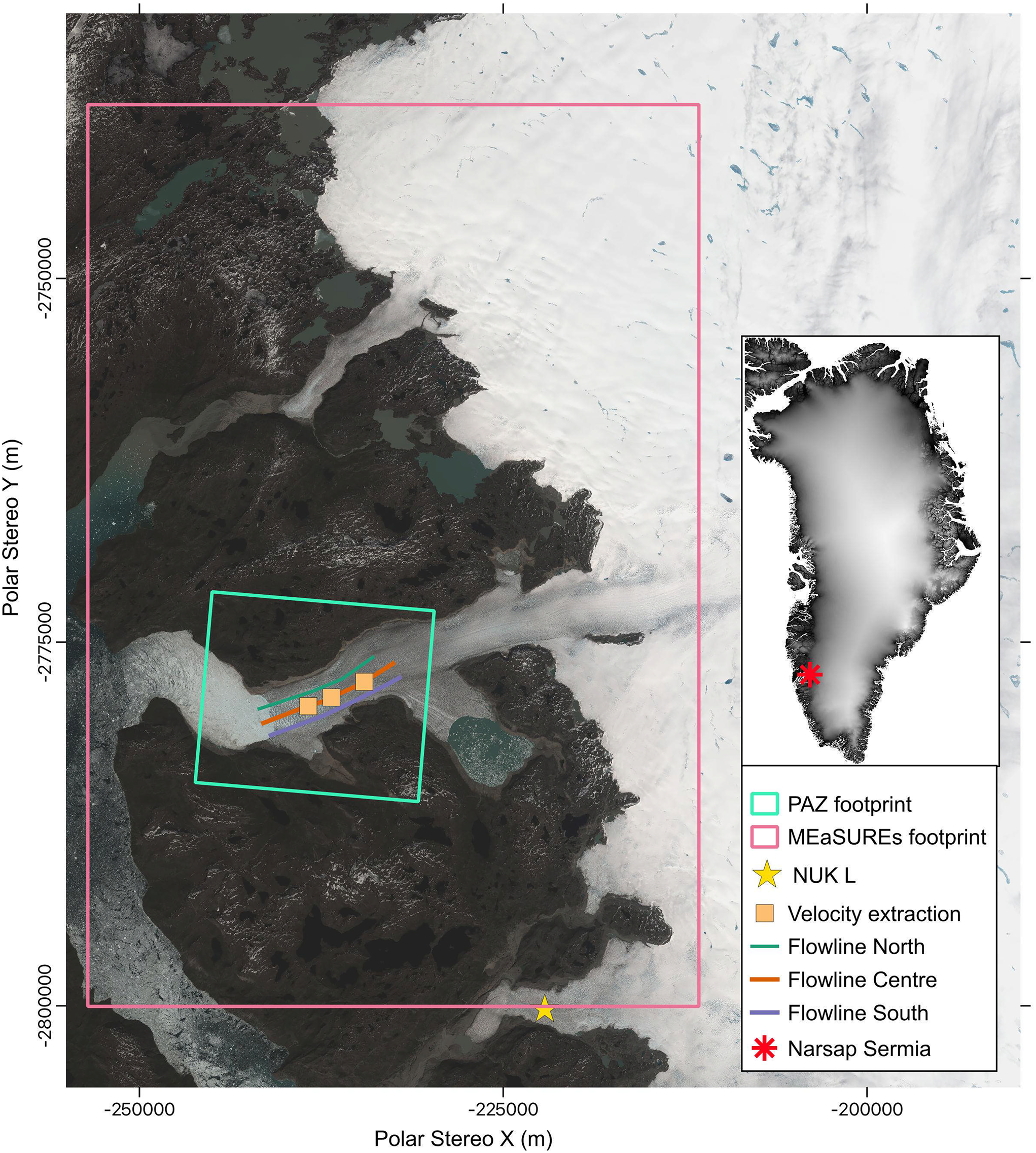
We use PAZ Ciencia spotlight mode Synthetic Aperture Radar data acquired between 30/10/2019 and 23/02/2021 with an 11-day revisit time, providing a total of 43 images. We derive 42 velocity maps using a daisy-chain approach (i.e. displacement between image 1 and image 2, displacement between image 2 and image 3, etc). The satellite is tasked to acquire data for a 12 km by 12 km area of interest (Fig. 1, turquoise box) in descending orbit with single polarisation and an incidence angle of ~32° at the centre of the scene. Spotlight mode was favoured as it can achieve a higher azimuth resolution and subsequently a higher overall spatial resolution (azimuth and range directions of 1.1 and 1.2 m; (HDS Team, 2019)). Data are delivered in single-look complex image format, and an ASTER DEM is automatically downloaded and subsequently up-sampled using an 2 m ArcticDEM strip for georeferencing.
Footprint of acquired PAZ Satellite Aperture Radar data (pink) and MEaSUREs Satellite Aperture Radar data (turquoise; Joughin and others, Reference Joughin, Smith, Howat, Scambos and Moon2010, Reference Joughin, Howat, Smith and Scambos2021) on top of Mosaic of European Space Agency (ESA) Sentinel-2 RGB images acquired on 09/07/2021. Inset map shows location of Narsap Sermia (red cross) on top of surface topography from BedMachine V4 (Morlighem and others, Reference Morlighem2017, Reference Morlighem2021).
Methods
Velocity
The Single Look Complex (SLC) spotlight mode data are processed using the open-source InSAR Scientific Computing Environment 2.2.0 (ISCE; Rosen and others, Reference Rosen, Gurrola, Sacco and Zebker2012) and, due to similar SLC data formatting and viewing geometries, we can apply the TerraSAR-X stripmap mode processing chain without modifications. To derive velocities, offsets between consecutive image pairs are computed through normalised cross correlation using the Ampcor module, and geocoded with a window width of 256 pixels, a search width of 88 pixels and a skip width of 30 pixels. These parameters are determined to be most suitable, based on velocities calculated in previous studies for Narsap Sermia (e.g. Motyka and others, Reference Motyka2017; Davison and others, Reference Davison2020), to capture pixel offsets between image pairs upstream of the terminus accurately.
As this study is looking at horizontal (i.e. surface parallel) velocities only, we assume no movement in the vertical direction (Moon and others, Reference Moon2014, Reference Moon, Joughin and Smith2015). Range offsets are sensitive to satellite to ground line-of-sight motion, which is quite steep (34-degree incidence angle) and hence sensitive to vertical motion. However, surface elevation changes at Narsap Sermia range between −2.6 and −6.3 m a−1 (2016 to 2018) and thus can be considered negligible as they are several orders of magnitude smaller (max Δh < 0.073 m per 11 days) than the resulting velocities (Studinger, Reference Studinger2014). The azimuth and range offsets are converted from radar coordinate pixel-spacing to geographic pixel-spacing by multiplication with the azimuth and range spacing (~1 m) to retrieve a pixel-posting of 16 m and an underlying true spatial resolution of 256 m. The resulting values are further transformed to East-West/North-South and flow parallel/perpendicular direction using 2-D vector rotation. For the rotation to flow parallel/perpendicular, we assume a flow direction of −135° measured from North for Narsap Sermia (with positive degree values to the West). The velocity magnitude is calculated, and a band-pass pass filter is applied to remove potential outliers (excluding top and bottom 0.5% of observations).
Velocities at the terminus and up to ~3 km upstream could not be captured, most likely due to the influence of changing mélange and near-terminus ice being calved between revisit times (Fig. S1). It was possible to identify these spurious velocities visually by (i) the presence of large velocity gradients between individual pixels, which is more associated with the movement of mélange (Amundson and others, Reference Amundson2010; Sutherland and others, Reference Sutherland2014); and (ii) areas where flow velocities show unrealistic values of ≫1000 m d−1 (Fig. S1). The identified areas of erroneous velocities have been masked out in grey on subsequent maps and figures and are excluded from the analysis.
Stacked median velocity and strain rate maps were created to provide an overview of the data, with the median being calculated using the cell statistics tool within ArcMap 10.7 (Figs 2, 6, S2). The stacked maps make it possible to identify areas of consistent high/low velocity and strain, which allows to put surface dynamics in relation to the underlying bedrock topography.
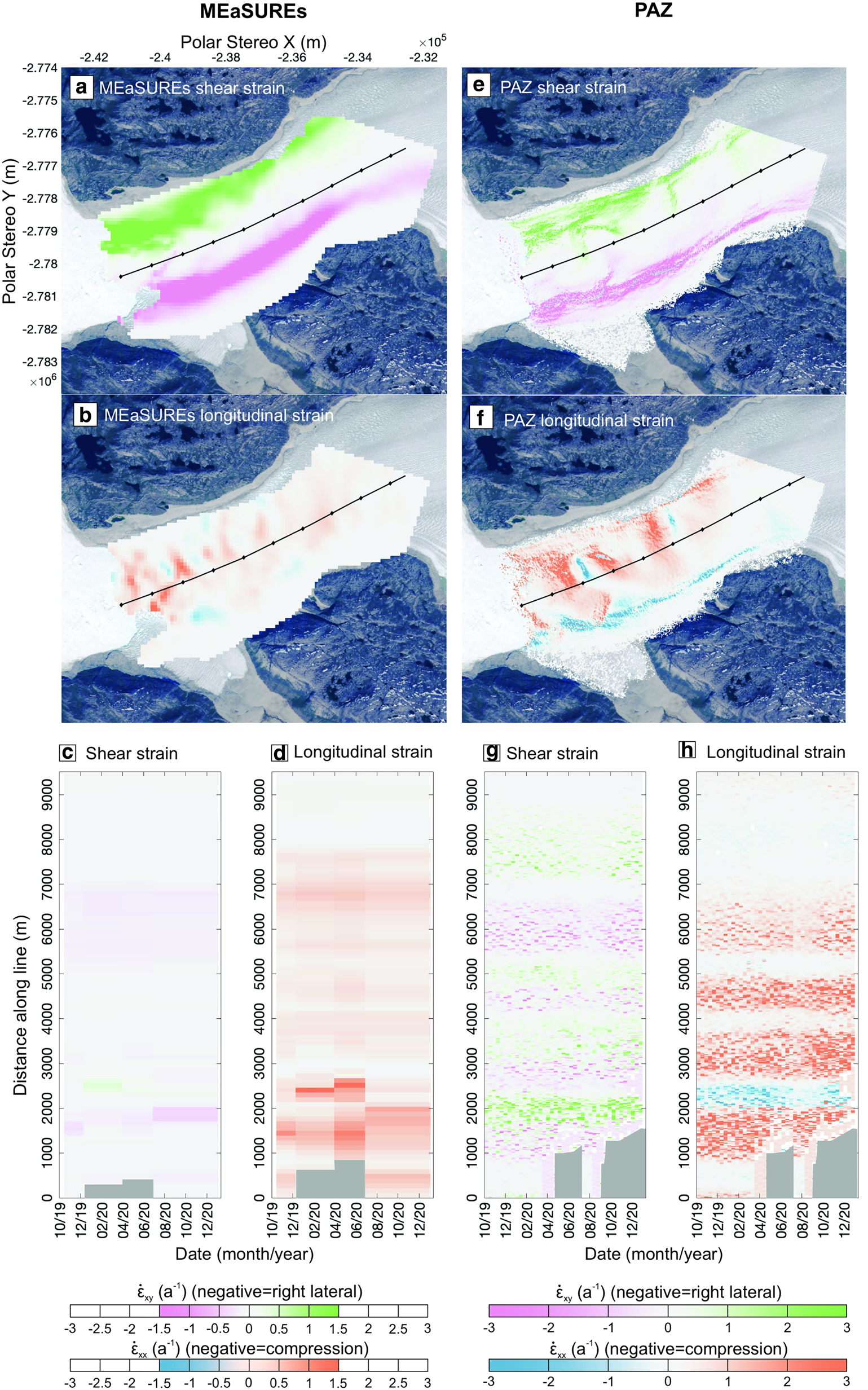
Comparison of shear and longitudinal strains derived from MEaSUREs SAR data (a–d) and PAZ SAR data (e–h) along the centreline with black ticks marking 1 km segments. Centrelines for MEaSUREs and PAZ data are shown in panels a, b and e, f respectively on top of stacked (median) shear and longitudinal strain rate maps (MEaSUREs strain rate posting is 100 m, PAZ strain rate posting is ~16 m). Basemaps show an ESA Sentinel-2 RGB image, acquired on 09/07/2021. NOTE: MEaSUREs data are shown with a different range. No-data areas are shown in light grey.
To show spatial differences in velocities over time, individual velocity maps for the period 12/4/2020 to 23/01/2021 were subtracted from the mean of the period 30/10/2019–01/04/2020, as this period showed relatively little variability and was thus considered to represent background winter velocities (Sole and others, Reference Sole2013; Tedstone and others, Reference Tedstone2015; Bartholomaus and others, Reference Bartholomaus2016).
Strain rate
Longitudinal, transverse and shear strain rates ($\dot{{\rm \varepsilon }}$ xx, $\dot{{\rm \varepsilon }}$
 yy, $\dot{{\rm \varepsilon }}$
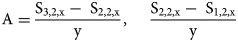
 xy) were calculated using the x and y velocity vectors which have previously been derived from azimuth and range offsets (posting 16 m). At its finest resolution, mean flow direction is calculated by taking data from 80 × 80 m blocks (5 × 5 pixels), before strain rate is calculated over a 48 × 48 m (3 by 3 pixels) sub-grid that is orientated ice flow parallel, with velocity values for each sub-gridpoint obtained through bilinear interpolation. The strain rate values calculated over the sub-grid are stored in a matrix Si,j with i rows and j columns, with the subscript indicating the position of the value within the sub-grid and the velocity vector used (x or y velocity vectors). Longitudinal ($\dot{{\rm \varepsilon }}$
 xx), transverse ($\dot{{\rm \varepsilon }}$
 yy) and shear ($\dot{{\rm \varepsilon }}$
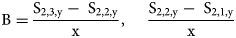
 xy) strain rates are then calculated as shown in Eqns (1)–(5).
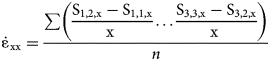
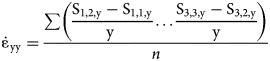
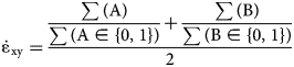
With n being the number of grid points and A∈{0,1}, B∈{0,1} being the conversion of A and B to logical values.
The PAZ derived strain rates were compared to strain rates derived from the National Snow & Ice Data Centre's (NSIDC) MEaSUREs version 4 velocities for the period 12/11/2019 to 02/05/2021 as an example of currently existing velocity data products (Joughin and others, Reference Joughin, Smith, Howat, Scambos and Moon2010, Reference Joughin, Howat, Smith and Scambos2021). In order to compare both data products, PAZ x and y velocities are recalculated to metres per year and reprojected to the polar stereographic grid. MEaSUREs x and y velocities, which are derived from TerraSAR-X/TanDEM-X SAR image pairs with an 11-day time difference between acquisitions, have a true resolution of several hundred metres and a posting of 100 m. The frequency of available MEaSUREs velocity products varies between a minimum of 55 days and a maximum of 187 days between sets of image pairs (Table 1).
Available MEaSUREs v.4 velocities derived from SAR data and the time interval in days between individual data products

Time series and outlier identification
Potential outlier pixels containing incorrect strains or velocities within the mélange are excluded by cropping the resulting maps using ice masks derived from tracing the glacier extent from each individual geocoded SAR image. Each SAR image is geolocated by co-registering all SAR images to the same PAZ reference image (image: 30/10/2019). The final mask used for each velocity acquisition is determined from whichever of the two masks from each image pair covered the smallest glacier extent.
Velocity values are extracted along a centreline and at 3.3, 5 and 7.5 km on the centreline, which have been determined to be locations with the least data gaps, to better visualise flow variability over time (Figs 1, S2). Strain rates are extracted along the centreline to enable the comparison between PAZ And MEaSUREs data (Fig. 2), and along lines in the northern, central, and southern sectors of the glacier to facilitate the analysis of PAZ derived strain rates through time (Figs 1, 6).
Bedrock topography is extracted for each line from BedMachine v4 with corresponding error estimates (Morlighem and others, Reference Morlighem2017, Reference Morlighem2021).
Terminus position and climate
Termini are digitised for each PAZ SAR image (Fig. S3) and margin change is quantified using the curvilinear box method within the Margin Change Quantification Tool (MaQiT; Lea, Reference Lea2018), with a box width equal to the width of the terminus (3200 m).
Air temperature data are taken from a PROMICE weather station (NUK_L), positioned on Qamanaarsuup Sermia approximately 25 km to the southeast from the centreline of Narsap Sermia at an elevation of 530 m a.s.l. (Fig. 1; Fausto and Van As, Reference Fausto, Van As and PROMICE Scientific Data2019).
Runoff is extracted and summed for the catchment of Narsap Sermia from daily MAR v3.11.2 (Modèle Atmosphérique Régional) data with a 6 km resolution (Fig. S4; Fettweis and others, Reference Fettweis2017; Mouginot and Rignot, Reference Mouginot and Rignot2019; Colosio and others, Reference Colosio, Tedesco, Fettweis and Ranzi2021). The MAR data do not account for subglacial runoff storage or transit times, therefore subsequent analysis assumes instantaneous runoff of meltwater.
Results
Comparison of PAZ and MEaSUREs SAR data
Figure 2 shows the comparison of shear and longitudinal strain rates derived from MEaSUREs and PAZ SAR data, which have been calculated over their respective velocity data postings of 100 and 16 m respectively.
The stacked shear and longitudinal strain rate maps show that both data products capture similar spatial patterns, but also reveal clear differences in the spatial distribution of strain rates (Figs 2a, b, e, f). For longitudinal strain rates, the spatial differences are most distinct at the margins, where PAZ data reveals an area of compression in the southern sector, whereas MEaSUREs data indicates close to zero strain rates. Spatial differences in shear strain rates are most apparent in the centre of the glacier, with PAZ indicating branches of left- and right-lateral shear towards the glacier centre (at ~3 and 6 km from the terminus), while the coarser resolution of the MEaSUREs data does not allow similar features to be identified. The differences are also apparent from the values extracted along the centreline transects, with local variations in strain rates in the PAZ data not being resolved by the MEaSUREs data.
The comparison of longitudinal strain rates between MEaSUREs and PAZ data shows that the overall patterns of extension (positive values) occur in similar locations for the entire observation period (Figs 2d, h). However, areas of compression (negative values) at ~2.5 and ~8 km from the terminus that are identified in the PAZ data are not resolved in the MEaSUREs data (Figs 2d, h). It is apparent that the higher spatial resolution PAZ data enables the identification of localised variability in strain rate that are not resolved in the MEaSUREs data.
Areas of right-lateral shear at ~3 and ~6 km from the terminus are more apparent in the transects of the PAZ data compared to MEaSUREs (Figs 2g, h). The high-resolution PAZ data are further able to capture considerably more complex distributions of shear strain rates along the flowline, with a zone of low right-lateral shear branching out across the glacier at ~7.5 km from the terminus (Fig. 2g).
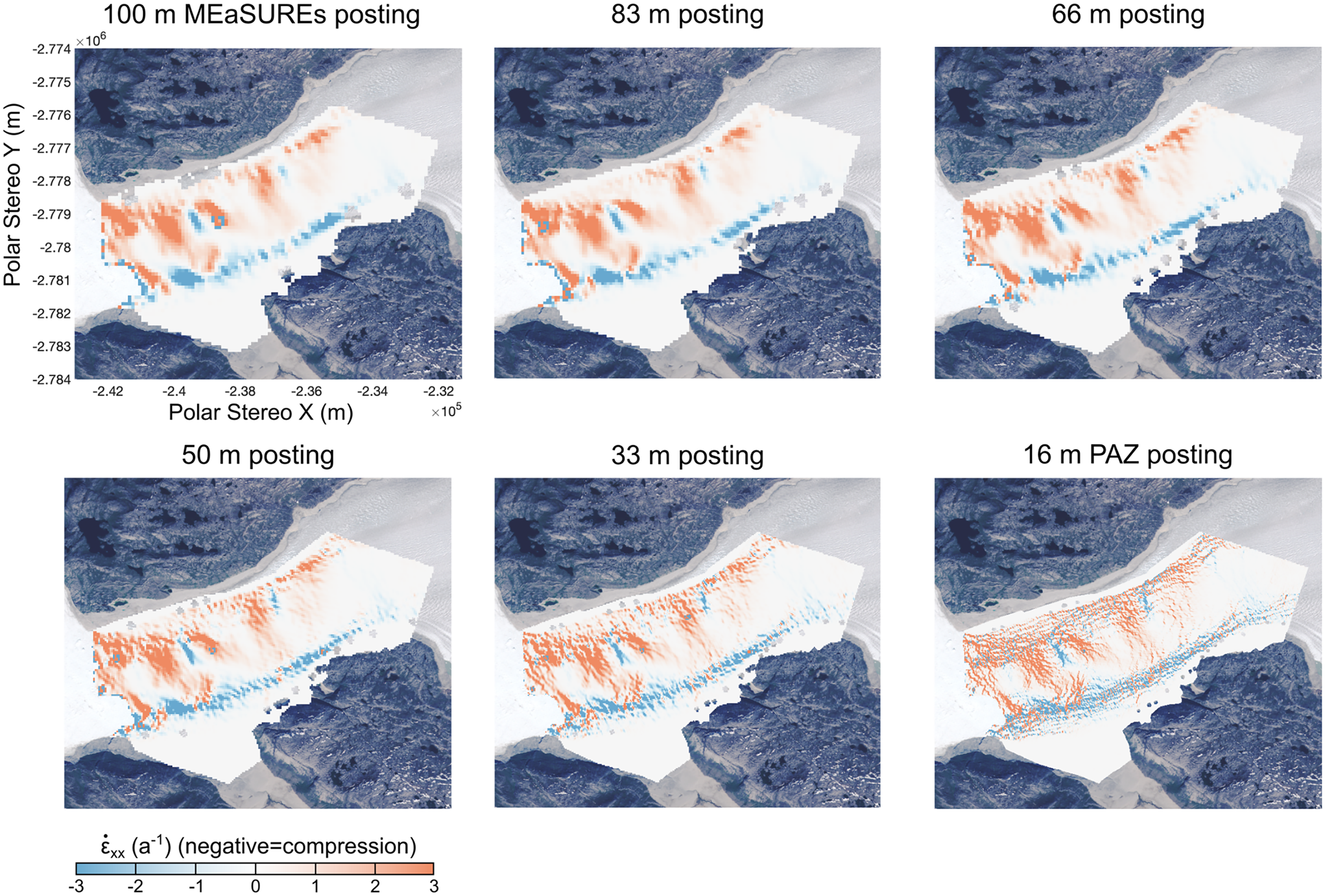
To illustrate how pixel-posting level impacts both the level of detail and values of strain rate derived, Figure 3 shows a longitudinal strain rate map of a PAZ velocity data acquisition (30/10/2019 to 11/11/2019) that has been continuously down sampled from its original resolution (16 m posting) to the MEaSUREs resolution (100 m posting). This highlights that 100 m resolution data generalises areas of compression and extension where those are the dominant signal, while high-resolution data reveal a much more complex pattern of local strain rate variability. As posting level becomes finer, the range of strain rate values is also found to increase substantially (Figs 2, 3).
PAZ SAR derived longitudinal strain rates (derived from image pair from 30/10/2019 and 11/11/2019) processed at different postings to highlight the difference between MEaSUREs data posting (100 m) and PAZ data posting (~16 m). Basemap shows an ESA Sentinel-2 RGB image, acquired on 09/07/2021.
Velocity evolution from PAZ data
The velocities derived from PAZ spotlight mode data show a general pattern of high velocities close to the terminus (~25 m d−1) and gradually decreasing velocities upstream (~5 m d−1 at 10 km from terminus; Figure 4). The velocity evolution of Narsap Sermia over the study period can be qualitatively categorised in four different stages (Fig. 4a):
Velocity evolution over time (30/20/2019 – 23/01/2021) from high-resolution PAZ SAR data (a) along the centreline with terminus position at the centreline shown in black and no data areas masked out in grey. (b) Velocities from points at 3.3 (circle), 5 (cross) and 7.5 km (diamond), respectively (Points shown in Fig. 1). (c) bedrock topography and errors extracted along the centreline from BedMachine v.4 data (Morlighem and others, Reference Morlighem2017, Reference Morlighem2021). (d) Air temperature from the PROMICE weather station NUK L, approximately 25 km to the southeast of Narsap Sermia. (e) Daily runoff for the Narsap Sermia catchment extract from MAR v3.11.2 (Mouginot and Rignot, Reference Mouginot and Rignot2019; Colosio and others, Reference Colosio, Tedesco, Fettweis and Ranzi2021). (f) Terminus position relative to the most recent observation computed in MaQiT. Yellow line shows start of the midsummer velocity slowdown.
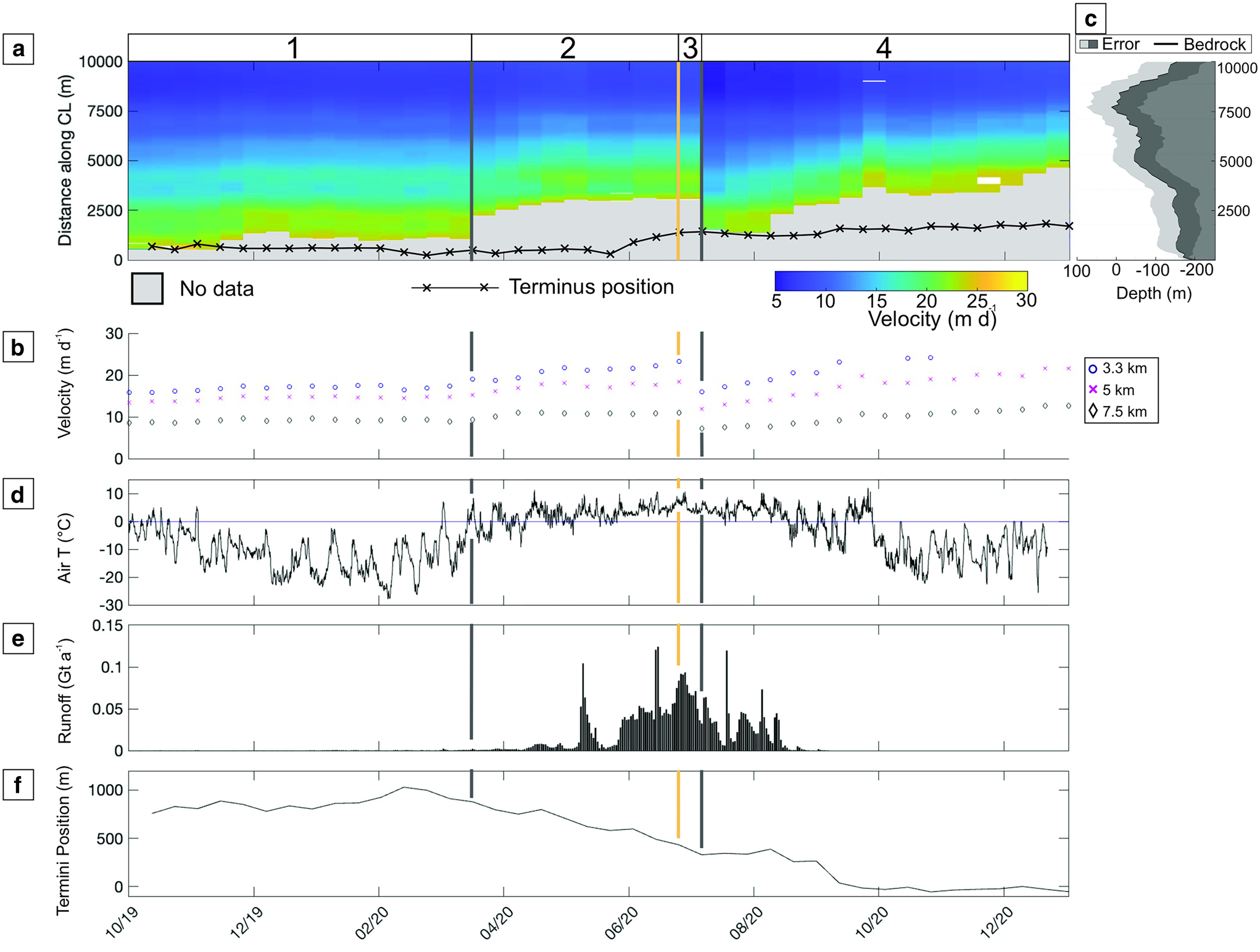
Stage 1 (30/10/2019–12/4/2020): Velocities remain steady from the start of the observational period in October 2019 until the beginning of April 2020, coinciding with a period where runoff is minimal or absent and air temperatures are below zero degrees. The terminus position remains stable from the start of the observation in October 2019 until January 2020, followed by an advance of ~200 m until mid-March and subsequent retreat of~120 m until the end of Stage 1 (12 April 2020).
Stage 2 (12/04/2020–31/7/2020): This stage coincides with the initiation of runoff, where an increase in flow velocities is observed, with the magnitude of this acceleration decreasing with distance from the glacier terminus (Figs 4a, c). Velocities reach their maximum in mid-May with speeds of ~22 m d−1 close to the terminus and ~10 m d−1 further upstream. This stage is characterised by positive air temperatures, with 92 out of 110 days experiencing temperatures >0°C (Fig. S5) at NUK_L weather station and runoff peaks in June and July. During this stage there is an overall terminus retreat of 550 m, punctuated by two small re-advances of ~50 m and ~16 m during the periods 4/05–15/05 and 17/06–28/06, respectively (Figs 4a, e).
Stage 3 (31/07/2020–11/08/2020): During this 11 day period a clear velocity slowdown is apparent, which is most pronounced at 3.3 km from the terminus (magnitude of deceleration ~7 m d−1) but can also be observed further upstream (~6 m d−1 at 5 km; ~5 m d−1 at 7.5 km; Figure 4c).
Stage 4 (11/08/2020–02/02/2021): Starting in mid-August, velocities gradually increase until the end of the observation period in February 2021. Runoff only occurs at the start of the stage and air temperatures begin to decrease with only 49 out of 154 days showing temperatures above 0°C (Fig. S5). Terminus retreat is apparent between 02/09 and 27/10 (~420 m), followed by relative stability and overall slight advance (~25 m) from 17/10 until the end of the observation period.
To illustrate the spatio-temporal patterns of velocity change, Figure 5 shows the differences between mean Stage 1 velocities (Fig. S2), and those of Stages 2 – 4. In Stage 2, velocity anomalies are initially high in the northern sector of the glacier and low in the southern sector of the glacier (12/04–23/04). This state is subsequently reversed, and velocities start to considerably increase from the southern sector of the glacier, with maximum velocity anomalies of >8 m d−1 being reached at the terminus. Negative velocity anomalies are however apparent in the northern sector along the lateral ice-bedrock border. The summer slow-down (Stage 3) is clearly apparent across the study area, with velocity anomalies being up to ~8 m d−1 lower than during Stage 2 and up to ~4 m d−1 lower than mean winter velocities (Stage 1). The onset of a positive velocity anomaly can be seen in the northern sector of the terminus at the beginning of Stage 4 (11/08/ – 22/08/2020), which subsequently propagates ~1 km upstream (02/09/2020) before spreading laterally across the glacier. By mid-September (13/09/2020), increased velocities reach the southern part of the terminus and encompass most of the near-terminus area. While it can be assumed that increased velocities are present in the near-terminus area, data gaps prevent definitively determining the extent of the acceleration close to the terminus (Fig. 5, Stage 4). The positive velocity anomalies propagate further upstream over time, so that increased velocities are apparent across the study area by the end of the observation period (03/02/2021). The data gaps increase in spatial extent over the period 22/08/2020 – 03/02/2021, which substantially limits the analysis of the acceleration between the terminus and ~3 km upstream.
Difference of velocities of Stages 2–4 to the mean of Stage 1 (for Stages see Fig. 4) with data gaps masked out in grey and terminus positions shown as blue lines. Basemap shows an ESA Sentinel-2 RGB image acquired on 09/07/2021.

Spatio-temporal strain rate evolution
There is a distinct separation between longitudinal strain rates in the northern and southern part of the glacier, with extension (i.e. longitudinal stretching; positive values) dominating in the central and northern sectors of the glacier (Figs 6c–e), and compression (negative values) being dominant in the southern sector of the glacier.
(a) Stacked longitudinal strains (median) with basemap showing an ESA Sentinel-2 RGB image, acquired on 09/07/2021. Location of strain extraction lines shown for the northern sector (green), the central sector (yellow) and the southern sector (light purple), black ticks marking 1 km segments, and location of small trough shown as purple rectangle. (b) Bedrock topography map (BedMachine v.4; Morlighem and others, Reference Morlighem2017, Reference Morlighem2021) with value extraction lines shown in red, black ticks marking 1 km segments, and location of small through shown as purple rectangle. (c–e) Temporal evolution of longitudinal strains for northern, central, and southern sector with corresponding bedrock topography and error (grey shaded). Boxes i–x show location of high strain, light pink dashed box shows location of small shelf and shallow through. No data areas are shown in light grey.
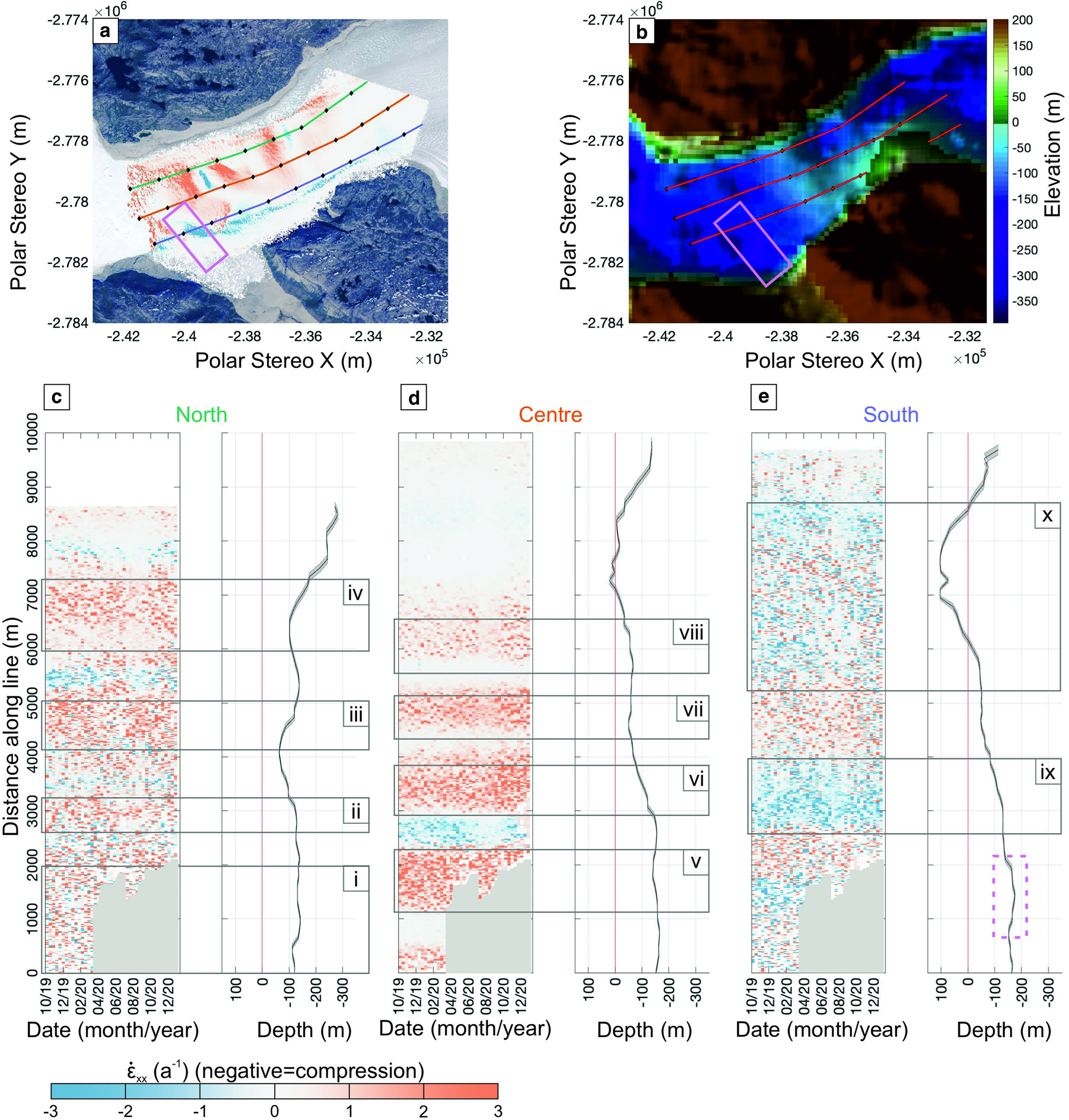
Extension in the northern sector is present near-terminus, and at ~3, 4.5 and 6.5 km from the terminus (Fig. 6c, ii–iv). A small area of compression is apparent at the start of an over-deepening (at ~7 km from the terminus) that extends further inland to a depth of ~400 m. Bedrock topography data along the flowline from BedMachine v4 suggests that subglacial topography is relatively flat at the terminus but shows local reverse bed slopes at ~3, 5 and 7 km from the terminus where we find extensional strain (Fig. 6c; Morlighem and others, Reference Morlighem2017, Reference Morlighem2021).
In the centre, we find four distinct bands of extensional strain rates at ~2, 3.5, 5, and 6 km from the terminus with their magnitudes decreasing with distance from the terminus (Fig. 6d, v–viii). Extensional strain rates are apparent on flat (Fig. 6d, v & vii) as well as reverse bed slopes (Fig. 6d, vi & viii).
In the southern sector (Fig. 6e), compressional strain rates are slightly more dominant in the first 2 km from the terminus, followed by intermittent bands off extension and compression up to 5.5 km from the terminus. Between ~5.5 and 9 km from the terminus we find a sector of high compressional strain rates, which coincides with a rise in local topography to ~100 m a.s.l. (Fig. 6e, x). An area of compression, which is apparent close to the terminus could correspond to the ice flowing over a small shallow trough (Figs 6a, b, e – dashed box). However, data gaps prevent tracking the evolution of the area of compression over the study period.
The evolution of strain rates shows little spatial variation over time (i.e. changes in sign of strain rate). In the south, strains are more compressional, though extensional strain values are also present whereas in the north and centre, extensional strains are more dominant (Figs 6c, d, e). Shear and transverse strains did not reveal any distinct spatial patterns or changes over time (Fig. S6). However, in the southern part of the glacier, bands of high left-lateral shear strain are apparent between 8 and 10 km from the terminus. This coincides with BedMachine v4 data suggesting that the bedrock topography is well above sea level (~100 m a.s.l.) and starting to slope in the direction of ice flow (Figs S6, 6).
Discussion
Comparison of PAZ SAR data with MEaSUREs resolution
The comparison of high-resolution PAZ SAR derived strain rates to MEaSUREs derived strain rates shows that the latter provide a general overview of the strain regimes but clearly simplify the spatial patterns of surface strain rates (Fig. 2). The results further reveal a difference in the range of surface strain rate values with higher values being derived from PAZ data.
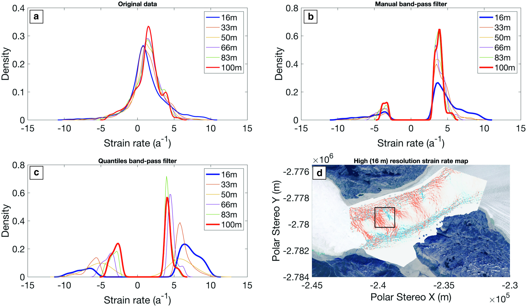
The kernel density estimation (KDE) plot in Figure 7a shows that medium-resolution data can capture broadly similar strain rate distributions for a given area of interest (Fig. 7d). However, it is quite apparent that strain rate extremes, which are highlighted in Figures 7b, c by applying a manually set (exclude values between −3 and 3) and quantiles based (25/75%) bandpass filter, are not captured by medium-resolution data. This provides a demonstration that coarser resolution data are likely to underestimate the magnitude of surface strain rates, especially for positive strain rates. For the cases shown in Figures 7b and c, positive strain rate distribution peaks identified in the high-resolution data are approx. 28 and 40% higher respectively, compared to data products with lower spatial resolution (Figs 2, 3; Rohner and others, Reference Rohner2019).
(a) Example of Kernel Density Estimation (KDE) for strain rates at different resolutions (PAZ resolution: 16 m; MEaSUREs resolution = 100 m). (b) KDE plot for strain rates with manually set bandpass filter (−3 to 3) for each data resolution. (c) KDE plot for strain rates with bandpass filter applied based on 25 and 75% quantiles. (d) Overview high-resolution (16 m) strain map with area of interest shown as black square. Basemap showing an ESA Sentinel-2 RGB image acquired on 09/07/2021.
Implications for calving, ice damage and implementation in ice sheet models
Our results confirm that obtaining strain rates from medium-resolution MEaSUREs data (length scales of 300 m) compared to finer scale PAZ data (length scales of 48 m) lead to a more smoothed impression of surface ice velocity which is not representative of TWG behaviour at length scales over which crevasses typically form (Borstad and others, Reference Borstad2012; Rohner and others, Reference Rohner2019). When constraining calving behaviour and ice flow in current ice sheet models, using strain rates derived from modelled or observed velocities with coarser posting levels (i.e. the order of 102 m) could result in the underestimation of key parameters such as ice damage, crevasse formation rates, crevasse depths, and the enhancement factor E (Borstad and others, Reference Borstad2012; Larour and others, Reference Larour, Seroussi, Morlighem and Rignot2012; Morlighem and others, Reference Morlighem2016; Rohner and others, Reference Rohner2019). These parameters are especially relevant in calving and diagnostic models, which aim to enhance our process understanding of calving behaviour, crevasse formation and ice damage evolution. For example, inverting for ice damage and in turn the enhancement factor E directly from medium-resolution velocity observations or model output could lead to an underestimation of both parameters thereby suggesting that higher stresses are required for calving to occur (e.g. Borstad and others, Reference Borstad, Rignot, Mouginot and Schodlok2013). Consequently, model simulations that are tuned to fit observations through basal inversions may be doing so by overestimating values of the basal sliding parameter.
For both calving and ice damage parameterisations within process level model simulations performed at grid scales of <102 m2, it is likely to be inappropriate to use strain rate extema derived at length scales that match model resolution. Instead, use of sub-grid extreme extensional strain rate values may reduce the level of tuning these parameterisations require to match observations by allowing the application of localised high strain rates and reducing the required tuning of the crevasse water depth parameter. While these sub-grid extrema cannot be applied directly, fine resolution observations of strain rate may be able to provide the basis for a generalised relationship. It is however worth noting that this would likely require a priori assumptions as to the appropriate length scales that both calving and ice damage occur over (Chudley and others, Reference Chudley2021). The results also have implications for strain-rate based calving laws. For example, the higher strain rate ranges derived from high-resolution data suggest that crevasses might reach greater depths than predicted by medium-resolution modelled and observational velocity data. Calving rates determined through crevasse-depth criterion based calving models could therefore require less tuning through the crevasse-water depth parameter (Benn and others, Reference Benn, Hulton and Mottram2007a), while tuning parameter values for von Mises-like calving laws may in reality be closer to unity.
In general, the results presented here indicate that currently widely available velocity data does not have the appropriate spatial resolution to either: adequately resolve ice damage or constrain and project calving behaviour on annual to seasonal timescales for strain rate based calving criteria within diagnostic ice sheet models.
Seasonal velocity changes
The seasonal velocity evolution at Narsap Sermia from Stage 1 to 3 is consistent with the findings of previous studies which showed that ice velocities are dependent on the influx of subglacial discharge and the evolution of the subglacial hydrological system (Sole and others, Reference Sole2013; Straneo and others, Reference Straneo2013; Motyka and others, Reference Motyka2017; Slater and others, Reference Slater2019; Davison and others, Reference Davison2020; Williams and others, Reference Williams, Gourmelen and Nienow2021). Specifically, Davison and others (Reference Davison2020) found that for the period 2014−2019, flow velocities at Narsap Sermia are characterized by an initial spring acceleration followed by a midsummer slowdown and subsequent recovery to pre-acceleration velocities throughout winter.
However, we find a highly local velocity increase at the northern terminus after the midsummer slowdown, which appears to initiate acceleration across the glacier, and results in overall high velocities throughout winter 2020/21 (Fig. 4, Stage 4). While data gaps at the terminus prevent to determine the spatial extent of the velocity increase in this region, it provides prima facie evidence that perturbations at the terminus are able to modulate velocity variations at medium sized, relatively shallow terminating Greenlandic glaciers (Lea and others, Reference Lea2014a, Reference Lea2014b), and not just large, deep terminating glaciers (e.g.(Nick and others, Reference Nick, Vieli, Howat and Joughin2009).
The sustained high velocities observed throughout winter 2020/21 indicate a dynamic change in the behaviour of Narsap Sermia as, compared to winter velocities between 2014 and 2019, velocities do not return to pre-spring acceleration magnitudes (Davison and others, Reference Davison2020). Davison and others (Reference Davison2020) found a similar, yet shorter (1–2 weeks), period of high velocities during January 2019 with air temperatures remaining negative and no runoff present during the period. The longer-term dynamic change found in this study occurs alongside comparatively high air temperatures, which are largely above 0°C until October (Fig. 4d), and no considerable subglacial discharge after mid-September which is consistent with data from previous years (Fig. 4e; Davison and others, Reference Davison2020). Similar to the brief winter acceleration found by Davison and others (Reference Davison2020), the data presented in this study, does not allow to attribute a distinct driver of neither, the perturbation at the terminus nor the subsequent sustained high winter velocities in 2020/2021. If, however, increased winter velocities are in fact the result of longer lasting periods of subglacial discharge caused by positive air temperature anomalies, Narsap Sermia could experience increased ice discharge and accelerated retreat in the future through higher winter flow velocities.
High-resolution longitudinal strain and bedrock topography
The analysis of longitudinal strain rates (Fig. 6) shows that over larger spatial scales (>102 m), strain rates are influenced by changes in bedrock topography and fjord geometry (Bassis and Jacobs, Reference Bassis and Jacobs2013; Enderlin and others, Reference Enderlin, Howat and Vieli2013; Catania and others, Reference Catania2018). A visualisation of flow direction (Fig. S7) shows that downstream of a topographic rise (~7 km from terminus), glacier flow is directed towards the south-southwest, whereas the fjord orientation is towards the southwest. This offset between fjord orientation and flow direction could explain the divergence in observed strain rate patterns between the northern and southern part of the glacier as apparent from Figures 6c and 6e. The results further show, that high longitudinal strain rates are predominantly present in the shallower part of the fjord (depths < 200 m) compared to almost no strain where topography indicates an over-deepened basin (Fig. 6c), which suggests that ice thickness is a control on the influence of bedrock topography on surface dynamics.
Over local spatial scales (<102 m), the results suggest that strain rates can be related to the underlying bedrock topography, with extensional regimes roughly following local high points (ridges) in the bedrock (e.g. Figure 6c, i–iv). These local variations in strain rates driven by topography could promote larger crevasse depths and thus have implications for calving laws as tuning parameters would need to be adjusted to these variations (Benn and others, Reference Benn, Hulton and Mottram2007a, Reference Benn, Warren and Mottram2007b; Borstad and others, Reference Borstad2012; Colgan and others, Reference Colgan2016). Past studies have shown that surface dynamics such as crevasse formation can be used to derive information about basal conditions (e.g. Colgan and others, Reference Colgan2016). Thus, strain rates derived from high-resolution velocimetry products could help to better constrain local bedrock topography for shallow grounded glaciers, provided that similar relationship can be found elsewhere (Fastook and others, Reference Fastook, Brecher and Hughes1995).
The analysis further revealed an area of compressional strain in southern part of the glacier, located ~1 km from the terminus over a local shallow trough. The compressional zone extends towards the centre of the glacier and extensional strains are present upstream (Figs 6a, h). If this compression zone persists, a perturbation could lead to a change in forces upstream, resulting in increased crevassing and ice damage, as suggested by previous modelling studies (Nick and others, Reference Nick, Vieli, Howat and Joughin2009; Lea and others, Reference Lea2014b; Brough and others, Reference Brough, Carr, Ross and Lea2023). However, as little change is observed over time and data gaps preventing the tracking of the strain rates for most of the study period, the development of this compressional zone remains highly speculative.
The results in this study show that high-resolution velocimetry data have the potential to provide new insights into bedrock topography, however, further research is necessary to establish definitive relationships between surface dynamics, crevasse formation and topography on local scales (e.g. Van Wyk de Vries and others, Reference Van Wyk de Vries, Lea and Ashmore2023).
Data availability and transferability
Some long-standing radar satellites, such as TerraSAR-X, Radarsat-2 or COSMO-SkyMed, have the capability to acquire SAR imagery with a high spatial resolution of up to 1 m, however swath widths are small compared to lower resolution modes (Werninghaus, Reference Werninghaus2004; Staples and Rabus, Reference Staples and Rabus2005; Fiorentino and others, Reference Fiorentino, Virelli and Battagliere2016). Newer SAR satellites like PAZ, ICEYE or UMBRA have made use of advances in technology to enable image acquisition with spatial resolutions of up to 0.25 m, yet swath widths remain similar (HDS Team, 2019; Ignatenko and others, Reference Ignatenko2020; UMBRA, 2024). Most high-resolution data are not freely available so that acquisitions need to be specifically requested or the data has to be commercially acquired, which, over larger spatial scales, requires considerable financial efforts. Therefore, high-resolution SAR data are currently not readily available for most tidewater glaciers in Greenland. While future advances in technology are anticipated to enable image acquisition with ever increasing spatial resolutions, ice-sheet wide high-resolution SAR imagery will most likely not become freely available in the foreseeable future. This might also not be necessary as findings derived from high-resolution data at one tidewater glacier can be transferred to other glaciers with similar characteristics.
For example, the results found in this study could be applied to other medium size, shallow grounded glaciers in Greenland. The observed increase in winter velocities at Narsap Sermia can be used as indicator for larger dynamic changes at tidewater glaciers initiated by a perturbation at the terminus (e.g. Nick and others, Reference Nick, Vieli, Howat and Joughin2009). This would be especially relevant for glaciers that experience a midsummer slowdown after spring acceleration (Type 2 glaciers, cf. Moon and others, Reference Moon2014), and comparatively high air temperatures after the midsummer slowdown.
The determined underestimation of longitudinal strain rate maxima further suggests that surface fracture mechanics (e.g. crevasse formation and depth, ice damage) at other glaciers might differ from what can be derived from medium-resolution data. Taking the findings of this study into account could lead to an improved understanding of the relationship between crevasse depth and calving at other glaciers.
Conclusion
This study presents detailed velocities and strain rates, posted at 16 m for Narsap Sermia derived from high-resolution PAZ spotlight mode SAR data (1 m resolution) for October 2019 to February 2021. These data reveal detailed spatial patterns of strain rate that are of higher magnitude and range than can be derived from medium-resolution data (Fig. 2), with substantial implications for constraining ice flow and calving behaviour of individual tidewater glaciers in ice sheet models. This is because using modelled or observed velocities at medium-resolution (e.g. 100 m) will translate to incorrect derivations of strain rate dependent parameters such as ice damage, crevasse formation rates and depths, and the enhancement factor E. As a result, diagnostic model simulation outputs that use strain rate based calving criteria and do not account for strain rate variability over shorter length scales than present may underestimate mass loss through calving. This is especially relevant for areas where the model resolution is higher than those of the input data.
We further find a spatial pattern of contrasting strain rates between the northern and southern part of the glacier, which appears to be related to a topography forced change in flow direction. This shows that basal topography and fjord geometry play a key role in the sign of strain rates (i.e. extensional or compressional), but current uncertainty around bedrock topography in Greenlandic outlets remains a key challenge to the understanding of this. In addition, the results presented here show that perturbations at the terminus can be a key driver of glacier dynamic change that can propagate upstream at small to medium size Greenlandic tidewater glaciers, which could not have been identified in lower resolution velocity products.
While high-resolution SAR imagery is not available for many tidewater glaciers in Greenland, the result presented here can be applied to other medium sized, shallow grounded glaciers and thereby provide further insights into their surface dynamics.
Supplementary material
The supplementary material for this article can be found at https://doi.org/10.1017/jog.2024.63.
Data
The processed velocity and strain maps as well as the digitised terminus margin data can be found at 10.5281/zenodo.10686530.
Acknowledgements
D. F. would like to acknowledge the support of this work through the EPSRC and ESRC Centre for Doctoral Training on Quantification and Management of Risk and Uncertainty in Complex System Environments Grant No. (EP/L015927/1). J. M. L. is supported by a UKRI Future Leaders Fellowship (Grant No. MR/S017232/1). P. J. G.'s work was partially supported by the Natural Environmental Research Council (NERC) through the Centre for the Observation and Modelling of Earthquakes, Volcanoes and Tectonics (GA/13/M/031). P. J. G. also thanks the Spanish Agencia Estatal de Investigación project PID2019-104571RA-I00 (COMPACT) funded by MCIN/AEI/10.13039/501100011033, and project PID2022-139159NB-I00 (Volca-Motion) funded by MCIN/AEI/10.13039/501100011033 and ‘FEDER Una manera de hacer Europa’. All high-resolution PAZ SAR images are part of the project: Evaluating the impact of PAZ spotlight mode data on tracking tidewater glacier dynamics and assessing the iceberg risk to Greenland's largest port (AO_001_019). The authors would like to thank two anonymous reviewers and the editor Hester Jiskoot for their constructive and helpful comments.
Author contributions
D. F., P. J. G. and J. M. L. conceived the study. D. F. processed the data, conducted all data analysis, figure production, and led the manuscript writing. J. M. L., P. J. G. provided conceptual and technical advice. J. M. L., P. J. G. and DWFM contributed to the writing of the manuscript.


 Open access