Data collection

A true testament to state politics, many of these data from 1990 to 2002 were obtained by contacting the states and, in most cases, by collecting the information from state legislative journals and blue books (also referred to as red or yellow books). While it was less difficult to attain party information for this period, the information on turnover was unavailable in most states. Countless states said this was not information they kept or collected. It is easier to list the states that had this readily available than those that did not. Those states were Texas, Minnesota (publicly accessible), and Florida (had to contact).

While the BOS is the premier source for much state data, the self-reported nature can lead to inaccuracies, especially with older information. For example, in the 1990s (and prior to), the Council of State Governments published the BOS biennially, which means there were years of lost data. The 1998–1999 version (vol. 32) included a page on legislative turnover (p. 70), but the listed turnover is after the 1997 elections. Very few states held elections in 1997, and special elections are not the only way that turnover occurs. So the influx of zeroes in this year is misleading. However, if you go to the preceding issue (vol. 31, 1996–1997), the numbers were counted after the 1994 election. This is a three-year gap resulting in a great deal of missing information. These are the numbers that have been used and relied on for decades. BOS has been and continues to be a great resource for state politics, but there are admittedly gaps. This is not an indictment of BOS, as this information is self-reported by each state, but there is a need for better consistency and record-keeping by states.

Some states do have membership databases, made possible by either the legislature or an outside third party (see the Supplementary Material). For the remainder of the states, we contacted various state officials and, in this process, were often directed to others. Research libraries, Senate Presidents and Clerks, House Clerks, Legislative Research Services, and numerous Secretary of State offices were all involved in this process. While some states were helpful and able to collate a list of turnover for this time period, most could only provide access to journals, many of which were only by session, with no continuous updates on members who may leave their term early.Footnote ⁸ In such instances, we were still able to track mid-term vacancies by reviewing roll call votes and session attendance records. We did find an overlap with professionalization, states that were most prepared to handle our request and had the most information to provide often overlapped with the states that are more professionalized.

On that note, there were some surprising gaps in the information provided. While California is one of the most professional states and has a large legislative staff, they do not track turnover of members, doubly surprising for a state with term limits where legislators are frequently removed. California does, however, have an assortment of historical files and databases. When we initially reached out to the California State Library, they said they had no information available other than California Blue Books, but suggested we could find the information from an article in Legislative Studies Quarterly (Moncrief, Niemi, and Powell Reference Moncrief, Niemi and Powell2004) or that we could find turnover for other states, and they included a link to Minnesota’s turnover chart.

For states that did not have turnover numbers to share, a database of lawmakers, or a complete list of members, we relied on state legislative journals, many of which are not available online. Different from the reported numbers from BOS, we were able to review individual journal pages and specific documents to individually track legislators. This process entailed listing each member in each district for more than 30 states, which was quite onerous, particularly for New Hampshire, with more than 400 members. This method allowed us to count the number of seats changing each year and session, to sort through the seat changes that occur post-redistricting.

The unfortunate drawback of states with session information only or where we filled the gaps is that the turnover statistics for the session/election year are likely inflated. We uncovered that turnover in session years was often recorded higher because some positions were filled in off-years and counted elsewhere. In other cases, there is the potential for underreporting as one individual might be appointed to fulfill the remainder of a term but then not seek reelection, and the seat would then be filled by someone else the following year.

From our perspective, the biggest issue is the lack of annual data and the tendency of the states to overly rely on individual session information. While session or election turnover has long been the standard practice, we can see from the collected yearly turnover information that people do leave in off years. We do not know if or how states account for this. Initially, we assumed we would have roughly half of the states with election year information only, because that was what the states could provide in the form of legislative journal rosters. We attempted to remedy this by tracking down information on mid-session vacancies, deaths in office, and by including special elections and appointments. Through this method, we were able to account for off years in all but one state, Connecticut.Footnote ⁹

Another issue was that of districts, both in terms of redistricting and the fact that a handful of states changed the number or makeup of districts over time. Redistricting at the state level is notoriously difficult, as it is not uncommon for members to be moved to a new district or drawn out. To counter this, we focused on the names of members and districts. If a member was moved to a new district but had no gaps in service, this was not counted as turnover. However, there were some instances where members would serve, leave, and then return – this was counted as turnover. Some states that had multi-member districts either dropped them and became single-member districts or adjusted the number of districts over time. For example, after Idaho redistricted in 1992, 21 seats were removed from the legislature.

Despite the difficulties and lack of consistency outlined above, we were able to amass a great amount of information.Footnote ¹⁰ Much credit is due to the responsiveness of a variety of contacts across the states. We find that the details of this particular endeavor and the methods of how to attain information can be just as important as the information itself. While turnover may not be of interest to everyone, varying state resources and access to information can have benefits among countless state and legislative scholars.

State example

In order to demonstrate some of the differences between our data and the BOS, we offer an example from Vermont. Oddly enough, Vermont appeared to be the perfect example of a state with good records, but records that were too detailed and ended up causing greater confusion. On the official state legislature website, there is an archived section that lists members by session between 1993 and 2014. Through inquiries, we learned that these lists were of members elected in the election preceding the session. However, these data were biennial, not annual.

Eventually, we were able to attain a copy of the Vermont General Assembly: Legislative Membership Roster 1966–2006 from the Senate.Footnote ¹¹ In this document, there is a list of the number of incumbents reelected in each election (by chamber) and the number of newly elected freshmen in each chamber (by election year). Taking the House, for instance, these numbers did not add up to equal the 150 seats in the chamber. This is a circumstance where there was a great deal of information, but it was conflicting information, and none of it was for off-years (non-election turnover).

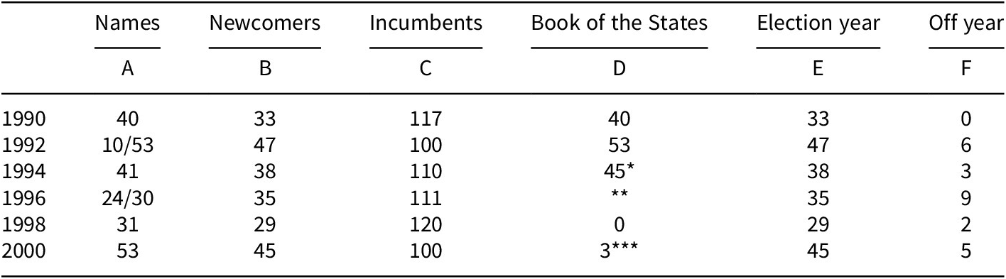
In order to gain information for non-election years, we used the list of names, as well as the number of incumbents and newcomers, to figure out how many people left in the off-year. Table 1 illustrates the differences in turnover numbers based on the information provided. Column A displays the number of names that were listed on the archived legislative site. This is in comparison to the list of newcomers (column B) and the list of incumbents (column C) provided in the “Legislative Membership Roster.” These numbers are offered in comparison to the BOS-reported turnover in column D. Taking all of the information provided, we were then able to differentiate between election-year turnover (column E) and off-year turnover (column F). While these numbers may appear somewhat similar at first glance, Table 1 illustrates the important differences in how turnover is reported in the states.

Table 1.

Discrepancies in vermont turnover, state house

Table 1. Long description

The table has seven columns: Year, Names, Newcomers, Incumbents, Book of the States, Election year, and Off year. For 1990, values are 40, 33, 117, 40, 33, 0. For 1992, 10 forward slash 53, 47, 100, 53, 47, 6. For 1994, 41, 38, 110, 45 asterisk, 38, 3. For 1996, 24 forward slash 30, 35, 111, double asterisk, 35, 9. For 1998, 31, 29, 120, 0, 29, 2. For 2000, 53, 45, 100, triple asterisk, 45, 5. Asterisks indicate special notes: single asterisk means published in the 1996 to 1997 volume, double asterisk means no report for 1996, triple asterisk means data reported after the 1999 elections and published in the 2000 to 2001 volume.

Note: *Published in the 1996–1997 volume, **no report for 1996, ***data reported after the 1999 elections and published in the 2000–2001 volume.

Part 1: Types of turnover in state legislatures

Measuring turnover

To best demonstrate the utility of SEAT and how it differs from previous measures and compilations of turnover, we first walk through the different ways that turnover is measured, and we then introduce our measurement.Footnote ¹² Following this, we illustrate the notable differences in how the type of turnover matters. This is not to say that existing measures of turnover are irrelevant, but rather, the type of turnover that is used ought to be theoretically motivated and the drawbacks well understood.

Of research on legislative turnover, session turnover is perhaps the most common measure as it has historically been the default. Session turnover relies on the start of a session as a reference point. Only newcomers for each legislative session are counted as an occurrence of turnover. The difficulty with this measure is that states have different session lengths, ranging from two to four years, which can result in lost information. The example below comes directly from Gouglas and Maddens (Reference Gouglas and Maddens2019, 104):

$$ \mathrm{Session}\ \mathrm{turnover}=\left(\mathrm{newcomer}{\mathrm{s}}_{\mathrm{s}\mathrm{ession}\ \mathrm{start}}/\mathrm{legislature}\ \mathrm{size}\right)\times 100. $$

The second most common measure is electoral turnover. Or as Moncrief, Niemi, and Powell (Reference Moncrief, Niemi and Powell2004) called it, “election to election” (361). While this measure improves upon session turnover, it only counts from the start of the session to the following election, see below. Despite its common usage, the individuals who leave outside of electoral changes are often overlooked:

$$ \mathrm{Election}\ \mathrm{turnover}={\displaystyle \begin{array}{l}\left[\left(\mathrm{membershi}{\mathrm{p}}_{\mathrm{session}\ \mathrm{start}}-\mathrm{membershi}{\mathrm{p}}_{\mathrm{p}\mathrm{ostelection}}\right)/\mathrm{legislature}\ \mathrm{size}\right]\\ {}\times 100.\end{array}} $$

A less common measure, but one worth noting, is the measure from Butcher (Reference Butcher2022) comparing natural and artificial turnover. Using annual turnover data and data on lawmakers who term out of office, Butcher is able to distinguish the number of lawmakers who are forcefully removed from office (artificial turnover) from those who leave for naturally occurring reasons (death, resignation, and electoral loss), see below:

$$ \mathrm{Natural}\ \mathrm{turnover}=\left[\left(\mathrm{exits}-\mathrm{termed}\ \mathrm{members}\right)/\mathrm{legislature}\ \mathrm{size}\right]\times 100, $$

$$ \mathrm{Artificial}\ \mathrm{turnover}=\left[\left(\mathrm{termed}\ \mathrm{members}\right)/\mathrm{legislature}\ \mathrm{size}\right]\times 100. $$

In contrast with these other measures, we offer total turnover, meant to count each individual leaving their seat in each year, thus capturing the total amount of legislative turnover. We fall in agreement with Matland and Studlar (Reference Matland and Studlar2004) who stipulated “turnover is not just about electoral loss – it reflects personal decisions, including advancement and retirement, and should be understood as such.” We not only account for total annual turnover, but we also do so for each legislative chamber.

Below is the formula used to calculate both forms of turnover. We rely on a variable we call seats changing. This variable is meant to capture each individual who occupies a single seat in any given year.Footnote ¹³ Different from other measures that evaluate turnover in the chamber as a whole, we count turnover at the chamber level.Footnote ¹⁴ Meaning, if a lawmaker leaves the lower chamber and is elected or appointed to the upper chamber, that is counted as turnover:

$$ \mathrm{Chamber}\ \mathrm{turnover}=\left[\left(\mathrm{seats}\frac{\mathrm{changin}{\mathrm{g}}_{\mathrm{chamber}\ \mathrm{year}}}{\mathrm{chamber}}\mathrm{size}\right)\times 100\right], $$

$$ \mathrm{Total}\ \mathrm{turnover}=\left[\left(\frac{\mathrm{lowerseats}\ \mathrm{changin}{\mathrm{g}}_{\mathrm{year}}+\mathrm{upperseats}\ \mathrm{changin}{\mathrm{g}}_{\mathrm{year}}}{\mathrm{legislature}}\mathrm{size}\right)\times 100\right]. $$

Differences in turnover

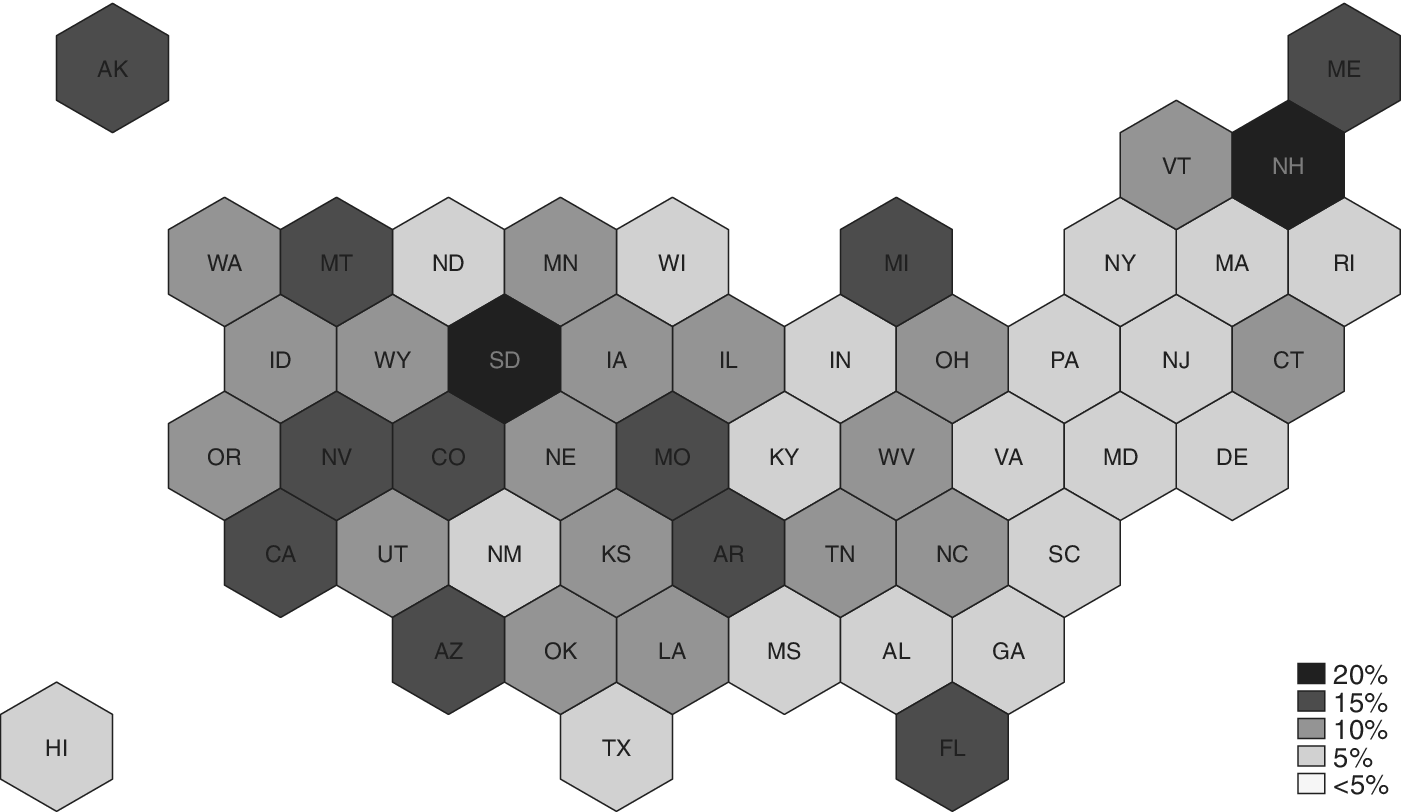
In Figure 1, we display the average percentage of turnover by state for the entire period encompassed in the dataset (1990–2020). When averaging all turnover across three decades, some results might be considered surprisingly high at around 20%; other states average roughly 5%. Again, this is an average of all turnover, electoral and not, across 30 years. High and low points are expected for each state.

Figure 1.

Percentage of turnover by state, 1990–2020.

Figure 1. Long description

Starting from the northwest, Alaska is shaded for 15 percent. Moving east, the northern states like Washington, Montana, North Dakota, and Minnesota are shaded between 10 percent and 15 percent. South Dakota, at the center, is the darkest shade representing 20 percent. New Hampshire and Maine in the northeast also show 20 percent. Florida in the southeast is shaded for 20 percent. Most other states are shaded in lighter tones, with the majority in the 5 percent to 10 percent range. The legend at the bottom right defines the shades: black for 20 percent, dark gray for 15 percent, medium gray for 10 percent, light gray for 5 percent, and white for less than 5 percent.

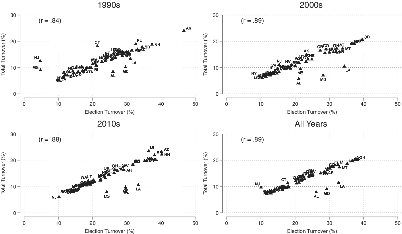
To illustrate the variance in the types of turnover, Figure 2 plots the differences in total versus electoral turnover for all states across three decades and for all years collectively. On the y-axis is the percentage of total turnover; electoral turnover is on the x-axis. If electoral turnover were a perfect mirror of the total turnover occurring in a state, then the relationship would be perfectly linear. Some states do appear to be so, but there are also clear outliers. We expect that electoral turnover is higher than total turnover when averaged over the decade, but these plots reveal instances where the two do not align. For example, in the 1990s, Mississippi and New Jersey’s total turnover was higher than the average electoral turnover, indicating lawmakers leaving in off years. In the 2000s, Alabama, Maryland, and Louisiana experienced much higher levels of election turnover and lower total turnover, meaning fewer people left in off years. Overall, the 2010s appear to be where there was the greatest level of consistency among the states in total turnover, mirroring electoral turnover, further validating BOS efforts. Whereas in the 1990s, the newest information reveals the greatest inconsistencies.

Figure 2.

Percentage of legislative turnover, by decade.

Figure 2. Long description

Top-left panel labeled 1990s shows Election Turnover percent on the x-axis from 0 to 50 and Total Turnover percent on the y-axis from 0 to 30, with r equals point eight four. State abbreviations are plotted as triangles, forming an upward trend. Top-right panel labeled 2000s has the same axes and range, with r equals point eight nine. State points are more tightly clustered along the upward trend. Bottom-left panel labeled 2010s, r equals point eight eight, shows a similar pattern. Bottom-right panel labeled All Years, r equals point eight nine, combines all data, maintaining the strong positive linear relationship. Outliers such as Alabama, Maryland, and Louisiana are visible in multiple panels. All axes are labeled Election Turnover percent and Total Turnover percent.

In the aggregate, the differences between total turnover and electoral turnover should not be that different. Total turnover is meant to encompass turnover that occurs during an election year. It is the instances where the two do not align that we can uncover more about individual state legislatures. While the reported Pearson’s correlation coefficient ( $ r $ ) for each decade is highly significant (p < 0.01), the addition of the missing years does make a difference for certain states. Notably, the decade with the weakest, albeit still strong, relationship is the 1990s.

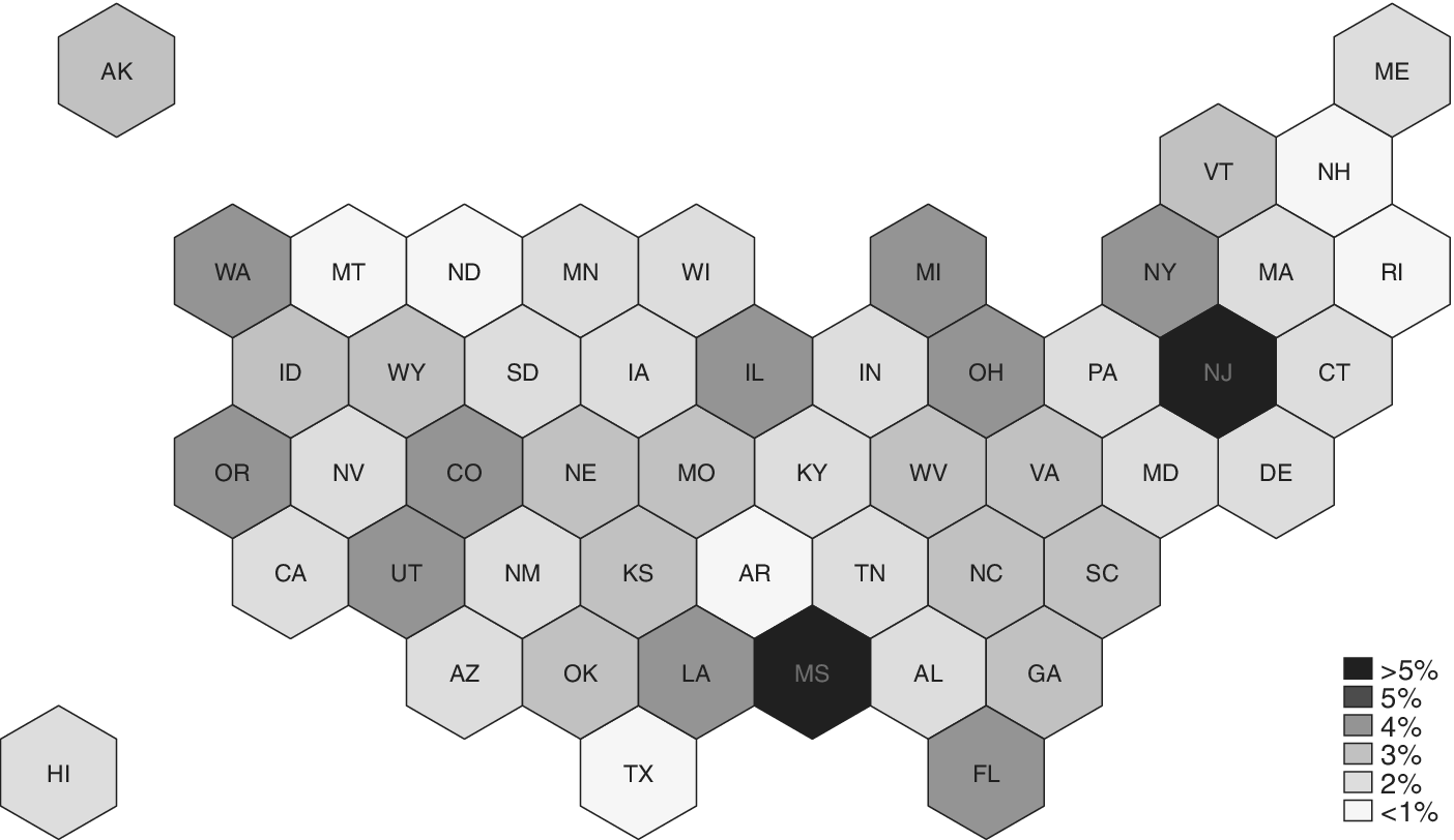
As a point of comparison, Figure 3 displays the percentage of legislative mid-session turnover from 1990 to 2020. This captures those who leave outside of the normal start of the session (or first day), where turnover is typically counted post-election. Different from the figure above, this displays only the members who leave at an atypical time, creating a vacancy in the legislature. Note that the scale for Figure 3 is from less than 1% to greater than 5%, with the average being 2.4%.Footnote ¹⁵ Disaggregating, there are 160 instances of a state/year having no openings in an off-year and 620 instances of turnover mid-session. Six hundred and twenty instances where members are typically overlooked.

Figure 3.

Percentage of mid-session turnover by state (vacancies), 1990–2020.

Figure 3. Long description

Starting from the northwest, each state is represented by a hexagon labeled with its postal abbreviation. The legend at the bottom right uses five shades from darkest to lightest: greater than 5 percent, 5 percent, 4 percent, 3 percent, 2 percent, and less than 1 percent. New Jersey and Mississippi are the darkest, indicating vacancy rates above 5 percent. States with 5 percent include Washington, Oregon, Utah, Colorado, Louisiana, and New York. States with 4 percent are Montana, California, and Florida. Most other states are in the 2 to 3 percent range, with the lightest shade indicating less than 1 percent, seen in states like South Dakota, Nebraska, and Maine. The map visually clusters higher vacancy rates in the West, South, and Northeast, with lower rates in the Midwest and northern Plains.

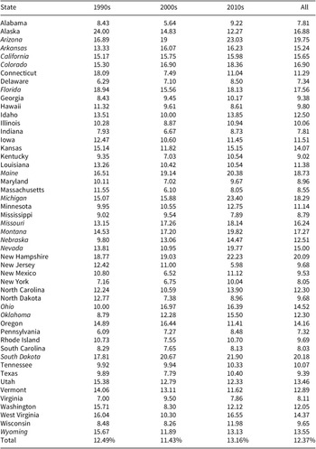
These data can also be used to evaluate each state, by decade, as seen in Table 2, which displays the average percentage of legislative turnover for each decade and the average across all 30 years. These percentages are derived from the total rate of turnover, not just the electoral turnover. By comparing a state’s 30-year average, we can see when a state had a decade with exceptionally high turnover, like Alaska in the 1990s, which was nearly double that of the national average. In the 2010s, Michigan and Arizona reached turnover rates nearly 10 percentage points higher than the average, though these shifts are largely attributed to term limits. There are also instances of abnormally low turnover. New Jersey averaged just below 6% in the 2010s, New Mexico (7%), and Alabama (6%) had turnover rates half that of the average in the 2000s. Similarly, Virginia, New York, and Delaware had half the rate of turnover as the 1990s average.

Table 2.

Average percentage of total turnover, by decade

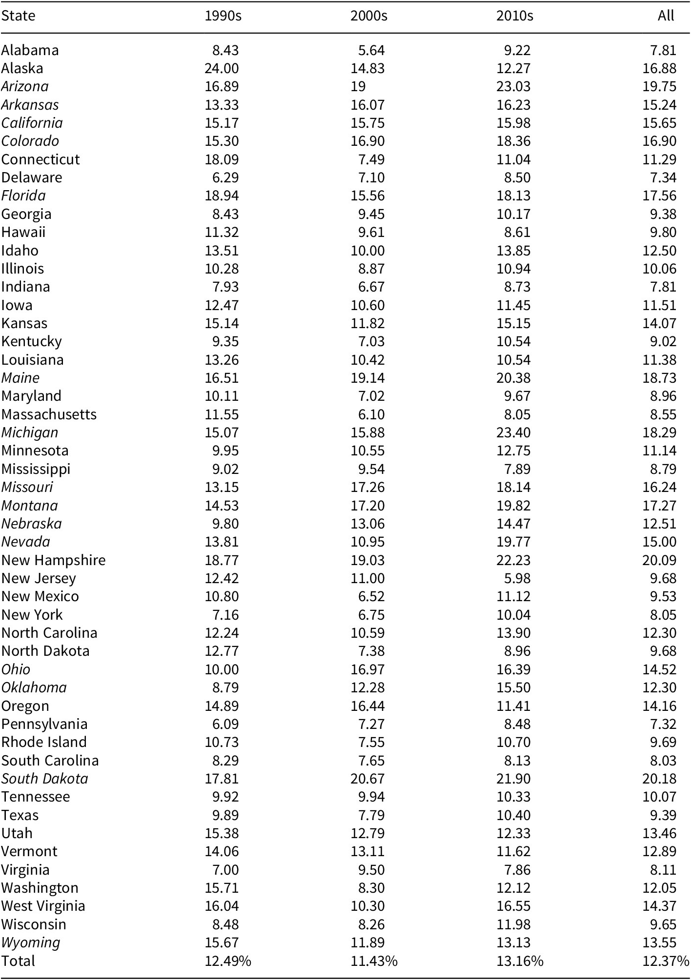
Table 2. Long description

The table consists of five columns: State, 1990s, 2000s, 2010s, and All. Each row lists a U S state, followed by its average percentage of total turnover for each decade and overall. Italicized states indicate term limits in effect prior to 2020. Alabama shows 8.43 for the 1990s, 5.64 for the 2000s, 9.22 for the 2010s, and 7.81 overall. Alaska has 24.00, 14.83, 12.27, and 16.88. Arizona (italicized) has 16.89, 19, 23.03, and 19.75. Arkansas (italicized) has 13.33, 16.07, 16.23, and 15.24. California (italicized) has 15.17, 15.75, 15.98, and 15.65. Colorado (italicized) has 15.30, 16.90, 18.36, and 16.90. Connecticut has 18.09, 7.49, 11.04, and 11.29. Delaware has 6.29, 7.10, 8.50, and 7.34. Florida (italicized) has 18.94, 15.56, 18.13, and 17.56. Georgia has 8.43, 9.45, 10.17, and 9.38. Hawaii has 11.32, 9.61, 8.61, and 9.80. Idaho has 13.51, 10.00, 13.85, and 12.50. Illinois has 10.28, 8.87, 10.94, and 10.06. Indiana has 7.93, 6.67, 8.73, and 7.81. Iowa has 12.47, 10.60, 11.45, and 11.51. Kansas has 15.14, 11.82, 15.15, and 14.07. Kentucky has 9.35, 7.03, 10.54, and 9.02. Louisiana has 13.26, 10.42, 10.54, and 11.38. Maine (italicized) has 16.51, 19.14, 20.38, and 18.73. Maryland has 10.11, 7.02, 9.67, and 8.96. Massachusetts has 11.55, 6.10, 8.05, and 8.55. Michigan (italicized) has 15.07, 15.88, 23.40, and 18.29. Minnesota has 9.95, 10.55, 12.75, and 11.14. Mississippi has 9.02, 9.54, 7.89, and 8.79. Missouri (italicized) has 13.15, 17.26, 18.14, and 16.24. Montana (italicized) has 14.53, 17.20, 19.82, and 17.27. Nebraska (italicized) has 9.80, 13.06, 14.47, and 12.51. Nevada (italicized) has 13.81, 10.95, 19.77, and 15.00. New Hampshire has 18.77, 19.03, 22.23, and 20.09. New Jersey has 12.42, 11.00, 5.98, and 9.68. New Mexico has 10.80, 6.52, 11.12, and 9.53. New York has 7.16, 6.75, 10.04, and 8.05. North Carolina has 12.24, 10.59, 13.90, and 12.30. North Dakota has 12.77, 7.38, 8.96, and 9.68. Ohio (italicized) has 10.00, 16.97, 16.39, and 14.52. Oklahoma (italicized) has 8.79, 12.28, 15.50, and 12.30. Oregon has 14.89, 16.44, 11.41, and 14.16. Pennsylvania has 6.09, 7.27, 8.48, and 7.32. Rhode Island has 10.73, 7.55, 10.70, and 9.69. South Carolina has 8.29, 7.65, 8.13, and 8.03. South Dakota (italicized) has 17.81, 20.67, 21.90, and 20.18. Tennessee has 9.92, 9.94, 10.33, and 10.07. Texas has 9.89, 7.79, 10.40, and 9.39. Utah has 15.38, 12.79, 12.33, and 13.46. Vermont has 14.06, 13.11, 11.62, and 12.89. Virginia has 7.00, 9.50, 7.86, and 8.11. Washington has 15.71, 8.30, 12.12, and 12.05. West Virginia has 16.04, 10.30, 16.55, and 14.37. Wisconsin has 8.48, 8.26, 11.98, and 9.65. Wyoming (italicized) has 15.67, 11.89, 13.13, and 13.55. The final row, Total, shows 12.49 percent for the 1990s, 11.43 percent for the 2000s, 13.16 percent for the 2010s, and 12.37 percent overall.

Note: Italics indicate states with term limits in effect prior to 2020.

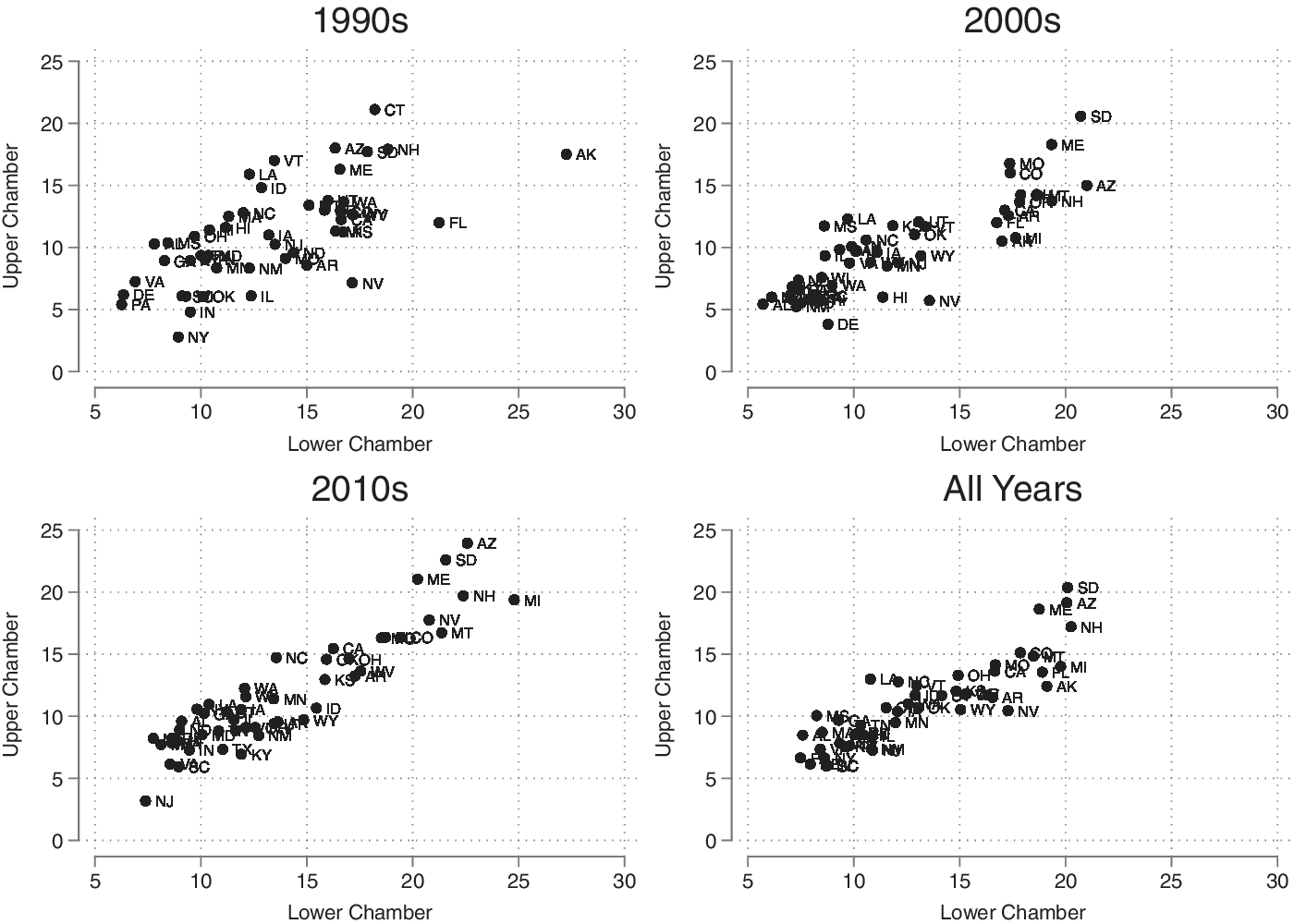
Alternatively, these data can be examined by chamber to capture some of the differences in desirability of service within each state. The plots in Figure 4 illustrate the shifts in legislative turnover across the decades. On the y-axis is turnover for the upper chamber, while the x-axis represents turnover in the lower chamber. Initial observations reveal linear trends in the 2010s, but turnover in the 1990s appears scattered. While some states are less distinguishable, the outliers are noticeable. In the 1990s, the number was higher for the upper chamber in several states, including Connecticut, Vermont, Arizona, and Louisiana. In the 2000s, there was a shift toward higher turnover in the lower chamber as seen in Nevada, Arizona, Michigan, and Florida, among others. When comparing with the percentages for all years, there are definite clusters. Nevada consistently has higher turnover in the lower chamber, as do Wyoming and Arkansas.

Figure 4.

Percentage of total turnover, by decade and chamber.

Figure 4. Long description

The layout consists of four scatterplots arranged in a two-by-two grid. Top-left is labeled 1990s, top-right is 2000s, bottom-left is 2010s, and bottom-right is All Years. Each plot has the x-axis labeled Lower Chamber, ranging from 5 to 30, and the y-axis labeled Upper Chamber, ranging from 0 to 25. Each point is labeled with a two-letter state abbreviation. In all panels, most states cluster along a diagonal trend from lower left to upper right, indicating a positive relationship between Lower and Upper Chamber turnover percentages. Outliers are visible in each decade: in the 1990s, AK and FL are separated from the main cluster; in the 2000s, SD and ME are highest on the y-axis; in the 2010s, A Z, S D, and ME are highest; in All Years, S D, M E, A Z, and NH are highest. The All Years panel shows the most compact clustering, with a few states (S D, M E, A Z, NH) as high outliers. The overall trend across decades is a consistent positive association between Lower and Upper Chamber turnover, with some states consistently above the main cluster.

These data do suggest that turnover rates between chambers are more linear in recent history, leaning toward higher turnover in state lower chambers in more recent years. For reference, the incumbency advantage in the US Senate is less stable than it is in the US House, but Congress has a lower rate of incumbency than state legislatures. These data, separated by chamber, allow for an exploration of the differences that exist within the legislature. Recent research emphasizes the differences between state legislative chambers (Makse Reference Makse2022), even though the chambers have often been treated as less different than bicameralism in Congress.

It is worth noting one significant shift that affects hundreds of lawmakers: term limits. When reviewing the trends for the 2000s in Figure 4, there is a noticeable gap in the results, present also in Figure 2, but less stark. Most of the states on the right-hand side of the plot are states with term limits. There are heightened levels of turnover in this group of states, which continued to grow throughout the 2010s. Looking at all years, there are three notable outliers – Arizona, South Dakota, and Maine (clustered on the far right) are all states with legislative term limits, so it should be no surprise that they have some of the highest turnover rates.Footnote ¹⁶

Part 2: Replication extension using SEAT

Legislative turnover in the 1990s is different from turnover in the 2000s and 2010s; to what extent does this matter? To test the implications of these new data, we offer a replication-extension evaluating the legislative factors that influence turnover rates. Our goal of replication was hindered by these data and the availability of replication files. Given this, we opted for a more recent publication to extend, rather than recreate a publication from 25 years ago. In “Parties and Professionals, An Exploration of Turnover in U.S. State Legislatures,” Jordan Butcher (Reference Butcher2025) explored the factors that can increase or decrease turnover, focusing on legislative professionalization and party. This analysis utilizes BOS data but only extends from 2002 to 2018, making it the perfect test to see if institutional factors matter differently over time.Footnote ¹⁷

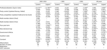
In addition to turnover data, this replication incorporates the updated professionalization measure from Squire (Reference Squire2024). We follow the same random-effects time series regression analysis as the original study, predicting the average rate of turnover by chamber. The results for 2002–2018 can be found in Table 3 alongside the replication with updated measures of turnover, professionalization, and party.

Table 3.

Replication analysis of parties and professionals

Table 3. Long description

Starting from the top row, the table lists variables in the leftmost column: Professionalization (Squire Index), Party control (Updated Ranney, folded), Party competition (Updated Holbrook and Van Dunk), Multi-member district (Post and Free), Four-year term, New electoral map, Government trifecta, Southern state, Constant, Observations, Number of states, Replication, and SEAT extension. For each variable, coefficients are presented for four periods: 2002–2018, less than 2001, greater than 2001, and all years, with lower and upper bounds for each. Robust standard errors are shown in parentheses beneath each coefficient. Significance is marked with asterisks: three for p less than 0.01, two for p less than 0.05, one for p less than 0.1. Professionalization shows strong negative coefficients for 2002–2018 (minus 13.173, minus 11.780, both with three asterisks), weaker negatives for earlier and later periods, and near zero for all years. Party control is negative across periods, with significance varying. Party competition is positive and significant in all periods, with coefficients ranging from 6.632 to 16.412. Multi-member district (Post) and (Free) show mixed coefficients, with some significant negatives. Four-year term and Southern state variables are mostly negative, with significance in select periods. New electoral map and Constant are strongly positive and significant. Observations and number of states are listed for each period, ranging from 510 to 1,479 observations and 47 to 49 states. Replication and SEAT extension rows indicate presence of asterisks for select periods. The table footnote clarifies robust standard errors and significance conventions.

Note: Robust standard errors in parentheses. *** p $ < $ 0.01, ** p $ < $ 0.05, * p $ < $ 0.1.

Using the SEAT data, we first focus on the differences present between turnover in the 1990s and the 2000s. Professionalization did not have an effect on turnover in the 1990s, but it did in the upper chamber in the 2000s. Professionalization takes time, and as states become more professionalized, the effect on turnover strengthens. There are two measures for party, competition and control. The effect of party competition on turnover is positive and significant in all models. Party control, however, varies depending on the decade and chamber. Centralized party control only decreases turnover in more recent history; the effects were not as prevalent in the 1990s in state lower chambers. Overall, parties have the greatest influence on turnover in state legislatures, with additional electoral effects of new district maps.

Next, we are able to compare the results using SEAT with the original data spanning 2002–2018. The findings indicated that term limits and professionalization decreased legislative turnover, while party competition increased turnover. In this update, however, professionalization does not appear to have the same lasting effect, especially for those who serve in the lower chamber. Last, party competition is the result that most closely aligns with the original analysis, whereas the strength of party control over time appears to have a greater effect on decreasing turnover. The question remains: What does this mean substantively?

Including additional data can reveal overlooked trends and new relationships. But the addition of data can also reveal a weakening or strengthening of existing relationships. Using the same regression results from above, we are able to test how much these measures matter by exploring the predicted average rate of turnover. We present two tests, one for each chamber, to demonstrate how the differences in measurement matter for substantive conclusions.

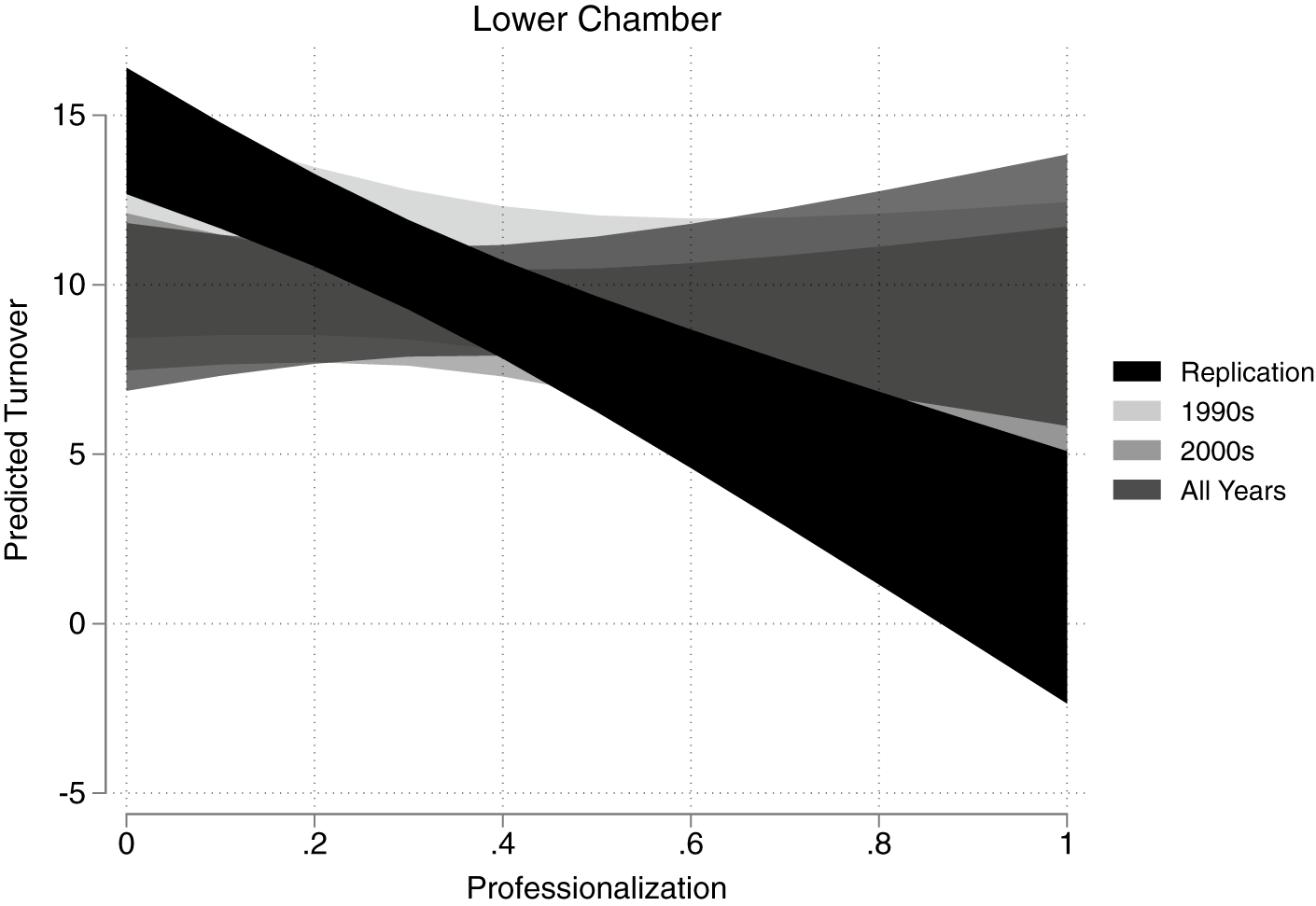
First, a test of professionalization for state lower chambers, which is one of the most inconsistent factors affecting turnover in Table 3. Figure 5 illustrates the extent to which professionalization can alter the predicted rate of turnover in state lower chambers, across four distinct measures. The darkest line is from Butcher’s original study, whereas the lighter lines utilize the newly updated data. As professionalization increases, the substantive effects, using these new data, is minimal at best.Footnote ¹⁸ While there is notable overlap among the new measures, which account for a longer period of time, the contrast with the original study is stark. As professionalization increases, there is the potential for a slight decline in turnover, but the outcome is different from the anticipated effects of a professionalized state.

Figure 5.

Predicted rate of legislative turnover, by level of professionalization.

Figure 5. Long description

The x-axis represents professionalization, ranging from 0 to 1. The y-axis is labeled predicted turnover, ranging from negative 5 at the bottom to 15 at the top. At the right, a legend identifies four bands: Replication (black), 1990s (light gray), 2000s (medium gray), and All Years (dark gray). The Replication band starts at about 15 predicted turnover at x equals 0 and slopes downward to about 5 at x equals 1, showing a strong negative trend. The 1990s, 2000s, and All Years bands are mostly flat or slightly increasing, with predicted turnover values between 7 and 12 across the x-axis. The shaded areas around each band indicate uncertainty, with the Replication band showing the widest range. The other bands overlap and remain above 5 predicted turnover throughout.

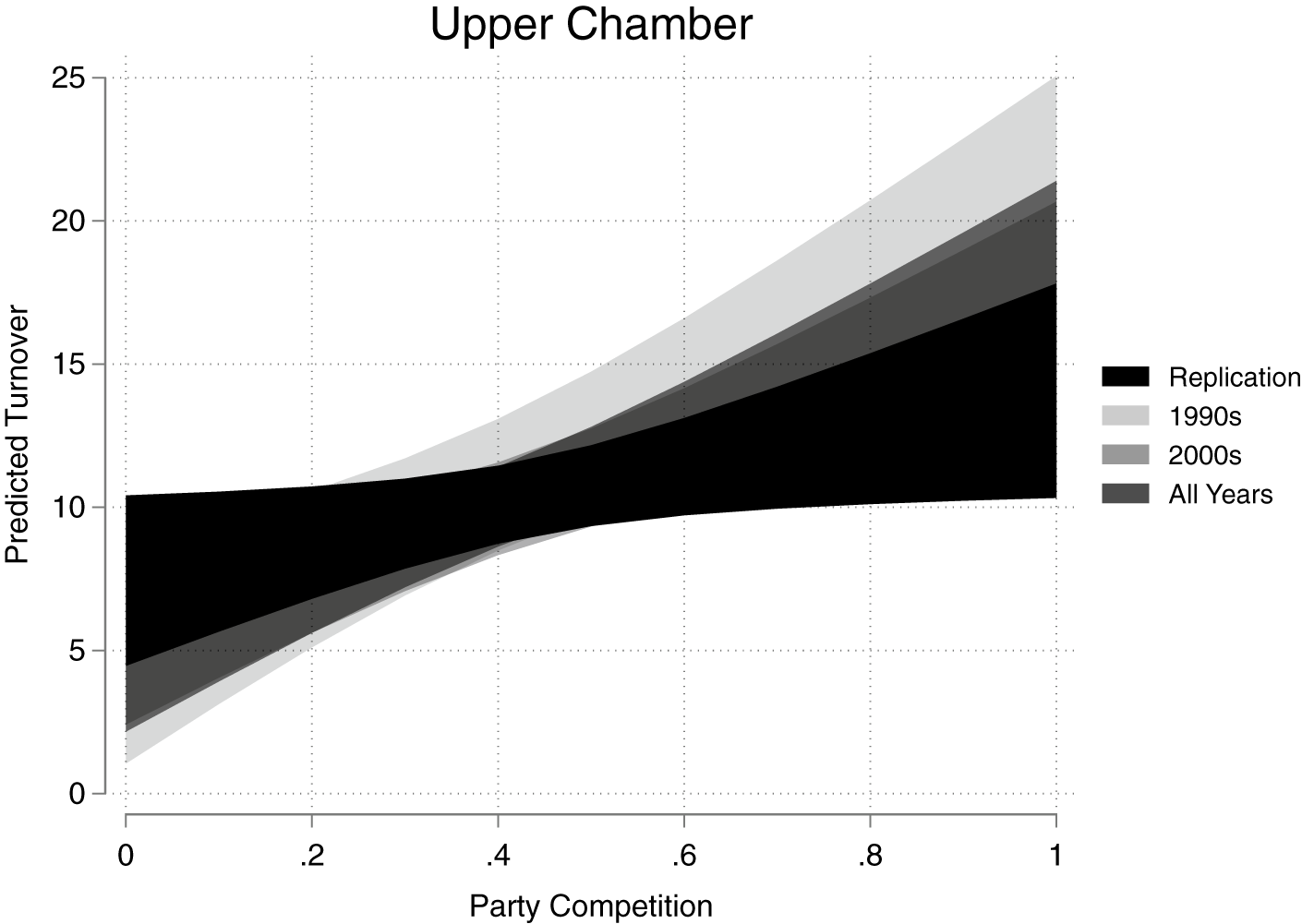
Also important to this story is party competition, which leads to turnover for the minority party. Our test of the upper chamber in Figure 6 actually reveals a stronger relationship between competition and turnover when using the extended data. Most notable is the shift that occurs in the 1990s, where turnover in a less competitive state was less than 5%, but as competition increased, so did turnover. Again, there is overlap between all four measures, but despite this, it is easy to see that the additional data points coincide with a clear, strong relationship between party competition and turnover. These results indicate that not only does turnover fluctuate over time, but the factors that most affect turnover shift as well. While the average rate for all states varied little between 1990 and 2020, there are notable differences in how turnover is affected by professionalization and party.

Figure 6.

Predicted rate of legislative turnover, by level of party competition.

Figure 6. Long description

The x-axis represents party competition, ranging from 0 to 1. The y-axis shows predicted turnover, ranging from 0 to 25. Four overlapping shaded bands represent different data subsets: Replication (black), 1990s (light gray), 2000s (medium gray), and All Years (dark gray). All bands show an upward trend, with predicted turnover increasing as party competition rises. The Replication band is the lowest, starting near 10 and ending near 15. The 1990s band starts just above 0 and ends above 25, showing the steepest increase. The 2000s and All Years bands fall between these, with All Years consistently above Replication but below 1990s. The legend on the right identifies each band by color.

This replication is one example of the numerous ways to use these data in state and legislative research. These data differentiate between turnover in the lower and upper chambers, while including the total turnover for the entire legislature. There are variables for the partisan breakdown in each chamber and the changes that occur from year to year. Other variables that may be of interest include the total number of legislative seats (by chamber) and the total number of seats that change each year. These variables make up the core of the dataset. Also included are indicators for multi-member districts (free versus post), redistricting cycles, new electoral maps, party control, and even the number of lawmakers removed by term limits.Footnote ¹⁹ Turnover can be used to explore how members shape outcomes, but also how external and internal forces affect turnover. Importantly, the added time component allows for a lengthier comparison of changes in the states.