


1. Introduction
Antarctic Ice Sheet mass loss is accelerating (Shepherd and others, Reference Shepherd2012, Reference Shepherd2018; Rignot and others, Reference Rignot2019), increasing its contribution to sea-level rise (Nerem and others, Reference Nerem2018). Most of the current excess mass loss is associated with the dynamic response of grounded ice to ocean-driven thinning or the collapse of ice shelves, which provide a backstress (‘buttressing’) opposing the seaward flow of grounded ice streams and glaciers (e.g. Dupont and others, Reference Dupont and Alley2005; Joughin and others, Reference Joughin, Smith and Medley2014). Observed acceleration of tributary glaciers following ice-shelf collapse (Scambos and others, Reference Scambos, Bohlander, Shuman and Skvarca2004) or thinning (Pritchard and others, Reference Pritchard2012; Joughin and others, Reference Joughin, Smith and Medley2014; Rignot and others, Reference Rignot, Mouginot, Morlighem, Seroussi and Scheuchl2014; Paolo and others, Reference Paolo, Fricker and Padman2015; Khazendar and others, Reference Khazendar2016) confirms the critical role of ice-shelf buttressing. Some amount of ice-shelf melting and calving is necessary to maintain the ice sheet in a steady state. However, mass loss at a faster than steady-state rate will reduce buttressing provided by an ice shelf.
Recent observations of rapid ice-shelf thinning have been attributed, primarily, to increased basal melting driven by strengthening intrusions of warm and salty Circumpolar Deep Water (CDW) into the ocean cavities under ice shelves in the Amundsen and Bellingshausen seas (Thomas and others, Reference Thomas, Jenkins, Holland and Jacobs2008; Jenkins and others, Reference Jenkins2010, Reference Jenkins2016; Pritchard and others, Reference Pritchard2012; Holland and others, Reference Holland, Bracegirdle, Dutrieux, Jenkins and Steig2019). Some ice shelves in this sector have experienced ocean-driven thinning rates exceeding 5 m a−1 (Pritchard and others, Reference Pritchard2012; Paolo and others, Reference Paolo, Fricker and Padman2015, Reference Paolo2018). These high thinning rates reduce traction at the sidewalls and basal pinning points, such as ice rises and rumples, leading to the retreat of grounding lines (Joughin and others, Reference Joughin, Smith and Medley2014; Rignot and others, Reference Rignot, Mouginot, Morlighem, Seroussi and Scheuchl2014; Shepherd and others, Reference Shepherd2018) and the seaward acceleration of grounded ice. For ice sitting on a retrograde bed slope – i.e. bed sloping downwards inland – this retreat can initiate a self-sustaining Marine Ice Sheet Instability (Weertman, Reference Weertman1974; Mercer, Reference Mercer1978; Schoof, Reference Schoof2007; Ritz and others, Reference Ritz2015).
The ice shelves that are currently thinning buttress grounded ice catchments represent potential contributions to sea-level rise exceeding 1 m (Joughin and others, Reference Joughin, Smith and Medley2014; Rignot and others, Reference Rignot, Mouginot, Morlighem, Seroussi and Scheuchl2014). However, the catchments with the largest potential contribution to sea-level change drain into large ice shelves that are currently close to steady state. Ross Ice Shelf (RIS), the focus of our study, is close to being in balance (Rignot and others, Reference Rignot, Jacobs, Mouginot and Scheuchl2013; Depoorter and others, Reference Depoorter2013; Moholdt and others, Reference Moholdt, Padman and Fricker2014); however, it buttresses ~11.6 m of total potential contribution to sea-level rise (Tinto and others, Reference Tinto2019), and geological records indicate that the ice-sheet's grounding line in this sector has changed substantially on millennial timescales (e.g. Naish and others, Reference Naish2009; Kingslake and others, Reference Kingslake2018; Anderson and others, Reference Anderson2014). The recent stability of RIS has been attributed to the insulation of the sub-ice-shelf ocean cavity from warm CDW intrusions by cold, dense water masses formed on the continental shelf (Dinniman and others, Reference Zumberge, Heflin, Jefferson, Watkins and Webb2011; Tinto and others, Reference Tinto2019). Basal mass loss is, instead, driven by subsurface inflows of cold, High Salinity Shelf Water (HSSW) that melts ice near deep grounding lines, and seasonal inflows of summer-warmed Antarctic Surface Water that melt shallow ice near the ice front (e.g. Assmann and others, Reference Assmann, Hellmer and Beckmann2003; Stern and others, Reference Stern, Dinniman, Zagorodnov, Tyler and Holland2013; Stewart and others, Reference Stewart, Christoffersen, Nicholls, Williams and Dowdeswell2019; Tinto and others, Reference Tinto2019). As a result, RIS may respond quite differently to projected climate changes than ice-shelves experiencing warm inflows of CDW.
Given the role of ice shelves in ice-sheet mass loss and sea-level change, we need to understand the different climate and dynamical mechanisms driving ice-shelf changes. It is now possible to develop approximately annual maps of ice-shelf surface height (e.g. Pritchard and others, Reference Pritchard2012; Paolo and others, Reference Paolo, Fricker and Padman2015; Sutterley and others, Reference Sutterley2019; Adusumilli and others, Reference Adusumilli, Fricker, Medley, Padman and Siegfried2020), and velocity (Rignot and others, Reference Rignot, Mouginot and Scheuchl2011; Fahnestock and others, Reference Fahnestock2016; Mouginot and others, Reference Mouginot, Scheuchl and Rignot2017a, Reference Mouginot, Rignot, Scheuchl and Millanb; Rignot and others, Reference Rignot2019; Yang and others, Reference Yang, Kang, Cheng and Yang2019). Interannual variability in ice-shelf height can then be compared with output from atmospheric and oceanic reanalysis models to identify relationships between climate forcing and ice-shelf responses (e.g. Paolo and others, Reference Paolo2018; Adusumilli and others, Reference Adusumilli2018, Reference Adusumilli, Fricker, Medley, Padman and Siegfried2020). On sub-seasonal timescales, that satellite-derived ice-shelf height change records cannot resolve, GPS arrays on ice shelves can be used to identify processes, such as tides (Padman and others, Reference Padman, Siegfried and Fricker2018) that cause high-frequency ice deformation and contribute to ice loss (Brunt and others, Reference Brunt, Fricker, Padman, Scambos and O'Neel2010, Reference Brunt and MacAyeal2014; King and others, Reference King, Murray and Smith2010, Reference King, Makinson and Gudmundsson2011; Makinson and others, Reference Makinson, King, Nicholls and Hilmar Gudmundsson2012).
Atmospheric and oceanic variability around Antarctica also includes a strong seasonal component that is unresolved by satellite-derived ice-shelf mass-balance products and undersampled by precise GPS observations limited to summer deployments. We assume, therefore, that an ice-shelf's response may also include a significant seasonal component. Here, we use data from a large-scale GPS array deployed on RIS in 2015 and 2016 to examine spatial and temporal variabilities of ice-shelf velocities. We compared GPS-derived velocities with the output from an ice-sheet model to test the hypothesis that the annual cycle of ice-shelf basal melt rates (Tinto and others, Reference Tinto2019) drives seasonal variability of ice-shelf velocities. We explore the similarities and discrepancies between the annual velocity cycles seen in the data and in the model output. Our analyses provide the modelling framework for future studies of RIS flow response to ocean variability, and associated changes in loss of grounded ice, at seasonal and longer timescales.
2. Ross Ice Shelf
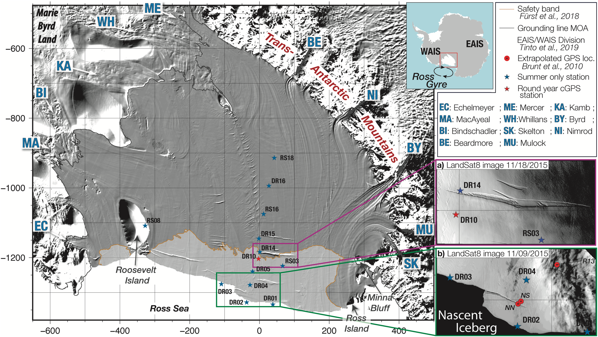
RIS in the southern Ross Sea, Antarctica (Fig. 1), is the world's largest ice shelf, with an area of ~480 000 km2. The ice shelf is fed by ice from grounded catchments of both the East and West Antarctic Ice Sheets (denoted EAIS, and WAIS, respectively) with a combined global sea-level rise potential of ~11.6 m (Tinto and others, Reference Tinto2019). Ice from the EAIS flows into RIS through narrow valleys in the Transantarctic Mountains (e.g. Stearns and others, Reference Stearns2011). Ice from the WAIS flows into RIS through six major ice streams (Shabtaie and Bentley, Reference Shabtaie and Bentley1987). The typical transit time for a parcel of ice to travel from the grounding line to the ice front is of order 1000 years, at typical speeds of several hundred metres per year. Most of the ice shelf is 300–500 m thick, with regions of thinner ice close to the ice front and thicker ice near the grounding lines of glaciers and ice streams (Tinto and others, Reference Tinto2019; Das and others, Reference Das2020).
RIS setting and location of GPS stations. (Main map) GPS network indicated by stars. Stations DR01, DR02 and DR03 appear in the Ross Sea because the mask for the background ice image (Antarctic REMA explorer, Howat and others, Reference Howat2019) is determined from the data acquired beginning in 2009 and is, therefore, not concurrent with GPS observations. Principal glaciers and ice streams are indicated by abbreviations; see the key in the upper right panel. The lighter ice-shelf shading near the ice front represents the ‘passive ice’ region from Fürst and others (Reference Fürst2016). Insets show November 2015 Landsat-8 images of (a) a major rift located between DR10 and DR14, and (b) the Nascent Iceberg and the ice-front stations compared to the position of GPS stations from Brunt and others (Reference Brunt, Fricker, Padman, Scambos and O'Neel2010) and extrapolated using the MEaSUREs ice-velocity field from Rignot and others (Reference Rignot, Mouginot and Scheuchl2017).
Ice-shelf mass balance is the sum of mass gained by flow across the grounding line and surface accumulation, and mass loss by iceberg calving and net basal melting. For RIS, a small fraction of basal melt under deep ice near the grounding line is refrozen under shallower ice in the central portion of the ice shelf (Zotikov and others, Reference Zotikov, Zagorodnov and Raikovsky1980; Adusumilli and others, Reference Adusumilli, Fricker, Medley, Padman and Siegfried2020). At present, the overall mass balance is approximately zero (Rignot and others, Reference Rignot, Jacobs, Mouginot and Scheuchl2013; Depoorter and others, Reference Depoorter2013; Moholdt and others, Reference Moholdt, Padman and Fricker2014), although there are regional patterns of variability in the surface elevation (Pritchard and others, Reference Pritchard2012; Paolo and others, Reference Paolo, Fricker and Padman2015, Reference Paolo2018; Adusumilli and others, Reference Adusumilli, Fricker, Medley, Padman and Siegfried2020). Following Rignot and others (Reference Rignot, Jacobs, Mouginot and Scheuchl2013), the mass balance for RIS averaged over several years consists of inputs of ~130 Gt a−1 of ice flow across the grounding line and 65 Gt a−1 of precipitation onto the ice shelf, and losses of ~150 Gt a−1 by iceberg calving and 60 Gt a−1 by basal melting. Averaged over the entire RIS, surface accumulation and basal melting rates are each ~0.1–0.2 m a−1 of water equivalent (Agosta and others, Reference Agosta2019).
Comparisons of ice velocities measured during the RIGGS project in 1973–1975 (Bentley, Reference Bentley1990) and modern satellite-derived values indicate substantial decreases in velocities in the southeastern corner of RIS near the grounding lines of Whillans and Mercer ice streams (Thomas and others, Reference Thomas2013), consistent with known changes in the behaviour of these ice streams. On a timescale of a few hundred years, MacAyeal and Bindschadler ice streams have exhibited variable velocities (Hulbe and Fahnestock, Reference Hulbe and Fahnestock2007), Kamb Ice Stream has been inactive for about the last 160 years (Retzlaff and Bentley, Reference Retzlaff and Bentley1993; Thomas and others, Reference Thomas2013), and Whillans and Mercer ice streams are both slowing down and could reach a state of near-stagnation within 50 years (Thomas and others, Reference Thomas2013). On shorter timescales (less than a few decades), ice stream velocities upstream of the grounding line can vary with subglacial hydrologic activity, as shown for Whillans and Mercer ice streams (Siegfried and others, Reference Siegfried, Fricker, Carter and Tulaczyk2016) and Byrd Glacier (Stearns and others, Reference Stearns, Smith and Hamilton2008). Flow changes of ice streams and glaciers can significantly affect the thickness of RIS: deceleration of grounded ice flow leads to ice-shelf thinning as ice influx decreases (Pritchard and others, Reference Pritchard2012; Campbell and others, Reference Campbell, Hulbe and Lee2018), while acceleration would lead to thickening of the ice shelf.
Substantial changes in the ice-front location may alter the stress balance and, therefore, the velocities of the ice shelf (e.g. Scambos and others, Reference Scambos, Bohlander, Shuman and Skvarca2004; Khazendar and others, Reference Khazendar, Borstad, Scheuchl, Rignot and Seroussi2015; Gudmundsson and others, Reference Gudmundsson, Paolo, Adusumulli and Fricker2019). Iceberg calving is primarily through the production of very large (scales of tens to hundreds of kilometres) tabular icebergs every few decades. The most recent major calving events occurred between 2000 and 2002 when nine giant icebergs were produced, with the two largest being B15 from the eastern RIS and C19 from the western RIS (Joughin and others, Reference Joughin and MacAyeal2005; Martin and others, Reference Martin, Drucker and Kwok2007; MacAyeal and others, Reference MacAyeal2008). The extension of the rift associated with B15 calving is projected to continue westward, eventually to result in the calving of a major iceberg (~20 × 40 km), called Nascent Iceberg (MacAyeal and others, Reference MacAyeal2006; Fig. 1b). However, because large icebergs tend to calve after the ice front has advanced north of the compressive regime imposed by northern Marie Byrd Land, Roosevelt Island, and Ross Island (Fig. 1), the mass loss causes a negligible decrease in buttressing (Fürst and others, Reference Fürst2016).
Ice-shelf dynamics can also be modified by changes in local mass balance (e.g. Joughin and others, Reference Joughin, Smith and Medley2014; Reese and others, Reference Reese, Gudmundsson, Levermann and Winkelmann2018; Gudmundsson and others, Reference Gudmundsson, Paolo, Adusumulli and Fricker2019). The surface and basal mass balance terms averaged over the entire ice shelf have similar values; however, they have distinct patterns of spatial and temporal variability. The surface accumulation is fairly uniform across the ice shelf, although it can change by a factor of 2–3 from one year to the next (Winstrup and others, Reference Winstrup2019). Basal melting is much more variable both in space and time (e.g. Tinto and others, Reference Tinto2019; Adusumilli and others, Reference Adusumilli, Fricker, Medley, Padman and Siegfried2020) and is, therefore, more likely to cause changes in ice dynamics. In addition, the mechanical strengths of fresh snow and firn layers are low because they have not yet gone through a complete process of compaction and solidification; therefore, they will tend to deform more easily than pure ice. Thus, we focus on changes associated with basal mass balance.
The current spatial distribution of basal melt rates for RIS is highly heterogeneous (Rignot and others, Reference Rignot, Jacobs, Mouginot and Scheuchl2013; Moholdt and others, Reference Moholdt, Padman and Fricker2014). Rates exceeding 10 m a−1 have been reported for the deep grounding line of Byrd Glacier (Kenneally & Hughes, 2004) and in a small subglacial channel near the grounding line of Whillans Ice Stream (Marsh and others, Reference Zumberge, Heflin, Jefferson, Watkins and Webb2016). Annual-averaged rates of order 1 m a−1 have been reported along the ice-shelf front (Horgan and others, Reference Horgan, Walker, Anandakrishnan and Alley2011; Moholdt and others, Reference Moholdt, Padman and Fricker2014; Stewart and others, Reference Stewart, Christoffersen, Nicholls, Williams and Dowdeswell2019), and along a narrow band of relatively shallow ice draft extending southward along the Byrd and Mulock glacier flowlines near Ross Island and Minna Bluff (Tinto and others, Reference Tinto2019). Averaged over the entire ice shelf, however, the basal melt rate is small, of order 0.1 m a−1 (Depoorter and others, Reference Depoorter2013; Rignot and others, Reference Rignot, Jacobs, Mouginot and Scheuchl2013; Moholdt and others, Reference Moholdt, Padman and Fricker2014), with melt rates being negligible for most of the ice shelf. The low area-averaged mass loss by melting is consistent with the low temperature of water masses on the Ross Sea continental shelf (e.g. Orsi and Wiederwohl, Reference Orsi and Wiederwohl2009; Pritchard and others, Reference Pritchard2012; Schmidtko and others, Reference Schmidtko, Heywood, Thompson and Aoki2014; Porter and others, Reference Porter2019).
Recent measurements by Stewart and others (Reference Stewart, Christoffersen, Nicholls, Williams and Dowdeswell2019) and modelling by Tinto and others (Reference Tinto2019) indicate, however, that the basal melt rates along the ice front and near Ross Island and Minna Bluff can change substantially at seasonal timescales. High melt rates, of order 10 m a−1, occur in summer when the upper ocean along the western RIS ice front is warmed by insolation after the sea ice has been removed by melting and advection (Porter and others, Reference Porter2019). The ice-shelf summer melting in this region dominates the annual average, suggesting that significant changes in summer conditions such as reduced sea ice could lead to substantial increases in annual-averaged melting. Sensitivity tests with an ice-sheet model (Reese and others, Reference Reese, Gudmundsson, Levermann and Winkelmann2018) suggest that localised ice-shelf thinning in this region could have a substantial impact on ice velocities over a large region, including grounded ice up to ~1000 km away at the WAIS grounding line of RIS.
Changes in mass loss from the grounded ice catchments around the RIS perimeter would require sustained (decadal and longer) increases in ice-shelf thinning rates (e.g. Reese and others, Reference Reese, Gudmundsson, Levermann and Winkelmann2018); however, as noted above, oceanic drivers of this thinning are seasonal. We, therefore, seek improved understanding of RIS dynamics, including at the seasonal and shorter timescales of the processes that may be relevant to long-term changes in ice-shelf mass balance.
3. Data and methods
3.1. GPS data and processing
A 13-station GPS array (Bromirski and Gerstoft, Reference Bromirski and Gerstoft2017) was installed on RIS in November 2015 as a component of the Dynamic Response of the RIS to Wave-Induced Vibrations (DRRIS) project. The GPS stations (Fig. 1) were collocated with seismic stations (Bromirski and others, Reference Zumberge, Heflin, Jefferson, Watkins and Webb2917), and remained in place for ~1 year. Three stations (DR01-DR03) were 2 km from the ice front, with DR02 being located on Nascent Iceberg (Brunt and others, Reference Brunt, Fricker, Padman, Scambos and O'Neel2010). Nine stations (including DR02) were positioned along a north–south transect from the ice front to ~430 km south (RS18), roughly aligned with the mean flow of the central ice shelf. Two additional stations were installed, one on the west side of this transect (RS03) and the other on grounded ice on Roosevelt Island (RS08). Twelve of the stations were powered only by solar panels, and consequently recorded data only during the two austral summers. One station, DR10, was continuously battery-powered and recorded during most of the experiments, including the winter months. The intervals of data acquisition at each site are shown in Figure S1.
All stations recorded at 1 Hz (1 sample s−1) and were processed following a precise point positioning (PPP) approach (Zumberge and others, Reference Zumberge, Heflin, Jefferson, Watkins and Webb1997; Geng and others, Reference Geng2012; Geng and others, Reference Geng2019) to generate, for every day, a 24-h time series with 1-s sampling. The horizontal movements were up to several metres per day. In order to merge daily time series into year-long continuous time series, we defined a reference position, per station, by estimating a static position (PPP) using the first 6 h of measurements of the first day of each time series. The 1-s time series were down-sampled to 30 s using a median filter, to create continuous time series over the entire time period.
3.2 MEaSUREs velocities
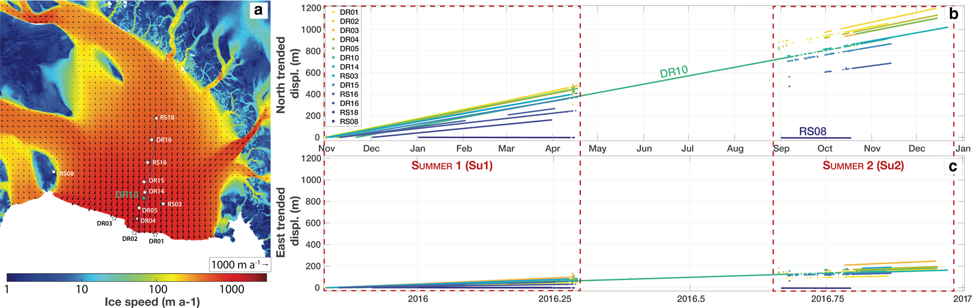
The Making Earth System data records for Use in Research Environments (MEaSUREs) project includes an Antarctic Ice Sheet velocity map (Rignot and others, Reference Rignot, Mouginot and Scheuchl2017) that was derived from data acquired between 1 January 1996 and 31 December 2016 from RADARSAT-2, Sentinel-1, TerraSAR-X, and TanDEM-X synthetic aperture radar (SAR), and Landsat-8 optical imagery. This dataset includes a long-term velocity field averaged over the 20 years of satellite data (represented in Fig. 2a), and annual velocity fields from 2005 to 2017.
Mean ice motion. (a) MEaSUREs ice-velocity field (shown by the colour scale) averaged over 20 years of data (Rignot and others, Reference Rignot, Mouginot and Scheuchl2017); vectors indicate the direction of flow. Horizontal (b) north and (c) east components of raw displacements (m) at each GPS station. Red boxes depict the two summers (Su1 and Su2) over which seasonal velocities were estimated (Table 1) and compared (Fig. 5).
3.3. Tidal analyses
Tides in the Ross Sea produce metre-scale vertical displacements of RIS (e.g. Brunt and others, Reference Brunt, Fricker, Padman, Scambos and O'Neel2010, Brunt and MacAyeal, Reference Brunt and MacAyeal2014; Padman and others, Reference Padman, Erofeeva and Fricker2008, Reference Padman, Siegfried and Fricker2018; Fig. S2). The horizontal components of displacements measured by GPS are dominated by the long-term averaged ice motion (Fig. 2; Table 1); however, in agreement with previous observations on RIS (e.g. Brunt and others, Reference Brunt, Fricker, Padman, Scambos and O'Neel2010, Brunt and MacAyeal, Reference Brunt and MacAyeal2014), the tidal signal is also significant (Fig. 3).
Tidal analysis of stations DR05 and DR10. Detrended time series of (a) north and (b) east components of GPS displacements (m) at stations DR05 (red) and DR10 (purple) compared to T_TIDE analyses (blue and yellow). (c) North and (d) east residual components at the same stations after removing tidal displacements using T_TIDE.

Locations and mean velocities of GPS stations. Longitude and latitude estimated over the first 6 h of measurements following each deployment. Mean north and east velocity components (in m a−1) over the whole records and for each of the two summers (Su1 and Su2; see Fig. 2b) are given. No data were obtained during Su2 for stations DR16 and RS18.

We identified the fundamental tidal signals (see Table S1 for the list of constituents) from the time series of vertical and horizontal displacements for each GPS record. To do this, we used the T_TIDE Matlab toolbox (Pawlowicz and others, Reference Pawlowicz, Beardsley and Lentz2002), which is based on the FORTRAN tidal analysis package developed by Foreman (Reference Foreman1977). T_TIDE provides a time series based on the tidal reconstruction from constituents that exceed a specified signal-to-noise (SN) ratio (we use SN = 1). The T_TIDE reconstruction of the vertical displacement in the year-long GPS record at station DR10 (Fig. S2) is very close to the predictions from the CATS2008 circum-Antarctic tide model (Howard and others, Reference Howard, Padman and Erofeeva2019), an updated version of the tidal inverse model described by Padman and others (Reference Padman, Fricker, Coleman, Howard and Erofeeva2002). The CATS2008 model assimilated, and therefore agrees with, GPS and satellite altimeter elevation data on RIS prior to 2009 (see Padman and others, Reference Padman, Erofeeva and Fricker2008), indicating that the vertical tide amplitudes and phase evaluated from our newer GPS records are close to their values prior to 2009. Temporal stability of tide height coefficients is consistent with the small variation in ice-shelf thickness and extent (e.g. Moholdt and others, Reference Moholdt, Padman and Fricker2014), which would otherwise drive changes in tidal fields (Padman and others, Reference Padman, Siegfried and Fricker2018).
We carried out T_TIDE analyses at all GPS sites, for all displacement components, and then calculated the predicted tides at each time series from the sum of all constituents whose amplitude exceeded SN = 1, with the exception of the semi-annual (S sa) constituent at DR10 (see discussion below). The longest continuous record lengths for all GPS stations, other than DR10, are ~4 months (first summer of observation, Figs 2b, c and Fig. S1). For records shorter than 6 months, tidal analyses cannot formally separate two pairs of closely-spaced (in frequency) large-amplitude tidal harmonics: semi-diurnals S 2 and K 2, and diurnals K 1 and P 1. To separate harmonics in each pair, we used a procedure called ‘inference’ (Pawlowicz and others, Reference Pawlowicz, Beardsley and Lentz2002), which is based on knowing the ratio of amplitudes and the phase differences of the two harmonics in the pair. We obtained the amplitude-ratio and phase-difference inference parameters for these pairs from our analysis of vertical motion at DR10, where the record is sufficiently long to separate these pairs explicitly. The inference parameters derived from DR10 for the horizontal displacements are similar to those for the vertical displacement.
Tidal analyses of solar-powered stations were undertaken only over the first summer since observations spanned a significantly shorter duration in the second summer (Figs 2b, c and Fig. S1). All time series are too short for us to obtain accurate estimates of the annual solar constituent, S a, even for the longer DR10 record. The semi-annual constituent, S sa, is formally resolved in the DR10 record by T_TIDE but, with less than two cycles measured, will not be reliably estimated in the presence of non-tidal sources of seasonal and longer-period variability. The annual cycle in the vertical component includes contributions from the seasonal cycle of atmosphere–ocean heat, fresh water and momentum exchanges. Based on the coastal tide gauge data from Scott Base (Ross Island) and a bottom pressure recorder in the northwest Ross Sea near the continental shelf break (Padman and others, Reference Padman, Erofeeva and Fricker2008), vertical amplitudes at S a and S sa periods are ~3 and 1–2 cm, respectively. These small amplitudes indicate that S a and S sa tides are not significant in the observed long-term variability in GPS heights (e.g. Fig. S2). Furthermore, these vertical signals are too small to provide significant forcing to the horizontal motion of the ice-shelf through nonlinear ice-ocean processes along the grounding zone, as suggested by Murray and others (Reference Murray, Smith, King and Weedon2007). The S sa constituent in the T_TIDE analysis of the DR10 horizontal displacement records is statistically significant (SN>1); however, including S sa produces a poor fit to the observed seasonal variability (Fig. S3), suggesting that it is an artefact of the T_TIDE algorithm when the record is too short to resolve S a concurrently with S sa. Therefore, we exclude S sa from the tidal fit for DR10. Murray and others (Reference Murray, Smith, King and Weedon2007) reported semi-annual variability in the lateral motion of grounded ice on Rutford Ice Stream on the southwestern edge of Ronne Ice Shelf, for a record which was sufficiently long (2 years) to allow formal resolution of both S sa and S a. However, their record is still too short, and poorly sampled in winter months when the GPS station was underpowered, to definitively assign a tidal origin to the fitted time series. We conclude, based on the lack of a visible S sa signal in our data from DR10, and the limited insights available from Murray and others (Reference Murray, Smith, King and Weedon2007) with regard to floating ice, that seasonal variability in the horizontal ice motion on RIS is most likely to be associated with non-tidal forcing on these timescales.
We used tidal analyses of the longer GPS records obtained during the first summer to predict and remove the tidal signals over the complete time series, including the second summer when records were shorter (see an example for station DR05 in Fig. 3). This allows for the removal of most of the fundamental tidal signals. Fortnightly signals remain, consistent with previous observations (e.g. Gudmundsson, Reference Gudmundsson2006; King and others, Reference King, Murray and Smith2010, Reference King, Makinson and Gudmundsson2011; Brunt and others, Reference Brunt and MacAyeal2014; Minchew and others, Reference Minchew, Simons, Riel and Milillo2017). However, our T_TIDE analyses did not find statistically significant oscillations at the precise frequencies of principal fortnightly tides (Table S1).
3.4 Ice-flow model
Ice-shelves thin locally when the ocean-driven basal mass loss exceeds mass gain from horizontal convergence, advection of thicker ice and local surface accumulation. This thinning can alter the dynamics of the ice shelf (e.g. Reese and others, Reference Reese, Gudmundsson, Levermann and Winkelmann2018). Depending on location, local thinning may also reduce buttressing of adjacent grounded ice catchments (Fürst and others, Reference Fürst2016; Gudmundsson and others, Reference Gudmundsson, Paolo, Adusumulli and Fricker2019). Here, we tested the impact of basal melting on the flow of the ice shelf by using the open-source ice-sheet and ice-flow model Elmer/Ice (Gagliardini and others, Reference Gagliardini2013), the glaciological extension of the Elmer finite element software developed at the Center for Science in Finland (CSC-IT).
We used the vertically integrated shallow-shelf approximation (MacAyeal, Reference MacAyeal1989), in which vertical shear stresses are assumed to be small relative to the horizontal longitudinal stresses so that the lateral ice velocity is constant throughout the ice thickness at each point. We calculated the effective ice viscosity as a vertically averaged quantity with a nonlinear dependence on strain rate, assuming isotropic material properties:

In Eqn (1), ɛe is the second invariant of the strain-rate tensor, η 0 is a vertically integrated apparent viscosity parameter (sometimes referred to as ice stiffness), and n = 3, the value most consistent with field data and most commonly used in ice-sheet modelling (Cuffey and Paterson, Reference Cuffey and Paterson2010). Bedrock elevation and ice thickness were taken from Bedmap2 (Fretwell and others, Reference Fretwell2013), with a surface elevation correction applied to the floating ice to ensure flotation for an ice density of ρ i = 917 kg m−3 and a water density of ρ w = 1028 kg m−3. The friction at the ice-bedrock interface was simulated with a linear Coulomb-like friction law, with a friction parameter (β) linking basal shear stress and sliding velocities (Cuffey and Paterson, Reference Cuffey and Paterson2010).
We conducted an inversion to infer β (for grounded ice) and η 0 (for both floating and grounded ice) that minimise a cost function (J V) measuring the discrepancy between observed and modelled velocities, for fixed ice-sheet and ice-shelf geometries (e.g. Fürst and others, Reference Fürst2015; Brondex and others, Reference Brondex, Gillet-Chaulet and Gagliardini2019). The observed surface ice velocity was taken from MEaSUREs 20-year averaged field (see Section 3.2). In addition, we simultaneously minimised a second cost function, J dh/dt, quantifying the difference between the ice-flux divergence and mass balance, to better constrain the inversion and keep the initial state closer to steady state (Mosbeux and others, Reference Mosbeux, Gillet-Chaulet and Gagliardini2016; Brondex and others, Reference Brondex, Gillet-Chaulet and Gagliardini2019). The mass balance accounts for the surface accumulation obtained from the Regional Atmosphere Model (MAR) averaged for the 1979–2015 period (Agosta and others, Reference Agosta2019), and the annual-averaged basal melt rates under the ice shelf extracted from the ocean circulation model reported by Tinto and others (Reference Tinto2019). A Tikhonov regularisation of both viscosity ($J_{\eta _0}$ ) and basal friction coefficient fields ($J_\beta$
 ), penalising the second derivative of each field, were included in the minimisation (e.g. Fürst and others, Reference Fürst2015; Brondex and others, Reference Brondex, Gillet-Chaulet and Gagliardini2019). The inversion then proceeded with minimising the following total cost function with respect to β and η 0:

where λ dh/dt, $\lambda _\beta \;$ and $\lambda _{\eta _0}$
 are constants allowing us to control the weight given to the different functions. The minimisation of J total (Eqn (2)) relied on the control method implemented in Elmer/ice and described by Gagliardini and others (Reference Gagliardini2013).
The inversion was conducted at the scale of the RIS basin, which encompasses the ice shelf and the grounded ice catchments that drain into RIS (Rignot and others, Reference Rignot, Mouginot and Scheuchl2011). We used a triangular finite element mesh with a spatial resolution that varies from 0.5 km at the grounding line to 20 km in regions of slow flow. The model spatial resolution on the ice shelf is typically ~2 km. A Neumann condition, resulting from the hydrostatic water pressure exerted by the ocean on the ice, was applied at the calving front (Gagliardini and others, Reference Gagliardini2013), while a Dirichlet condition forced the normal velocities to zero on the inland boundary of the basins adjacent to RIS.
The initial state is not perfectly steady due to remaining uncertainties in model parameters and initial conditions (e.g. the ice-sheet geometry used for the initialisation), which leads to non-physical ice-thickness rates of change and associated velocity variations during early stages of transient simulations (Seroussi and others, Reference Zumberge, Heflin, Jefferson, Watkins and Webb2011; Gillet-Chaulet and others, Reference Gillet-Chaulet2012). Following other studies, we conducted a relaxation simulation during which the ice-thickness rates of change decreased until reaching physically acceptable values in regard to the mass balance (e.g. Gillet-Chaulet and others, Reference Gillet-Chaulet2012; Brondex and others, Reference Brondex, Gillet-Chaulet and Gagliardini2019). This step consists of alternately re-solving the shallow-shelf equation and the advection of the ice thickness, accounting for basal melt rate and surface mass balance. The time needed for a model to reach a quasi-steady state that allows detection of the expected response to subsequent forcing perturbations is called the ‘relaxation time’. We note that the relaxation time required for our study of seasonal response (250 years; see Section 4.2) is substantially longer than in most studies that are focused on the ice sheet and ice shelf changes over decades or centuries (e.g. Gillet-Chaulet and others, Reference Gillet-Chaulet2012; Brondex and others, Reference Brondex, Gillet-Chaulet and Gagliardini2019).
After relaxation, we forced the model for 3 years with monthly basal melt rates from the ocean model described by Tinto and others (Reference Tinto2019). We note that this model was developed using a repeated annual cycle of forcing for the period 2001–2002 and so does not account for known interannual variability in atmospheric, oceanic and sea-ice conditions in the Ross Sea, including the likely effect of the 2016 El Niño event that was active during the period of GPS measurements. The annual average melt rates from the monthly snapshots are equal to the time-averaged fields used for the initialisation and relaxation steps. The 3-year period was chosen to assess the seasonal repeatability of the process and to identify potential remaining transients in ice flux (i.e. small local ice thickness and velocity variations) after the relaxation period, given the revised forcing associated with adding in seasonal variability.
4. Results
4.1. Variability in GPS-based position and velocity
4.1.1. Mean ice velocities
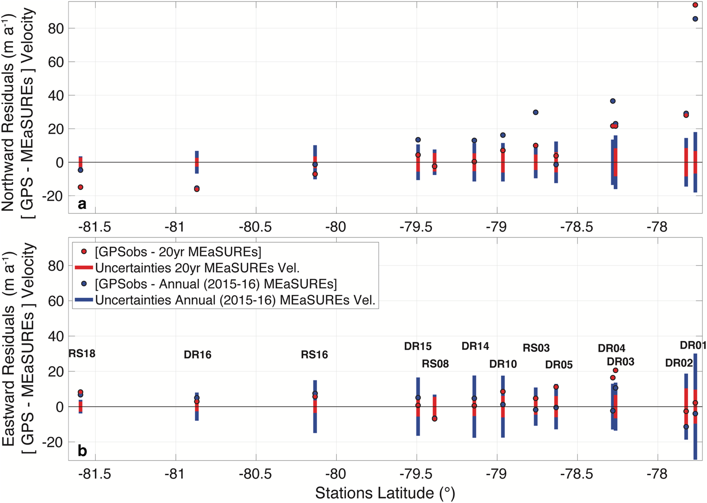
We estimated the mean horizontal ice velocities for each site (Table 1) for the complete record (about a year, including both summer periods of record for summer-only stations), using a linear least-squares fit to displacements after removing statistically significant tidal constituents (Section 3.3). RS08, which is grounded on the western flank of Roosevelt Island, recorded a small velocity (~8 m a−1) over the entire record: this site will not be further discussed in this paper. We compared our GPS measurements with the MEaSUREs 20-year averaged ice-velocity field (Rignot and others, Reference Rignot, Mouginot and Scheuchl2017, Fig. 2a) and with the MEaSUREs annual field concurrent with our GPS measurements (2015–2016) (see Section 3.2). Overall, the MEaSUREs and GPS velocity fields are in good agreement (Fig. 4). The largest discrepancies were observed for the ice-front stations, where GPS velocities exceeded the MEaSUREs values by 20–90 m a−1. These differences are most likely due to extrapolation from the MEaSUREs grid to the actual GPS positions. The grid for ice-shelf extent in MEaSUREs velocity products was based on data recorded prior to our measurement program when the ice front was farther south, causing the ice-front station locations to appear north of the MEaSUREs ice front and precluding direct comparisons (Fig. 2). Changes associated with the widening of the rift behind Nascent Iceberg could also explain some of the velocity differences between MEaSUREs and DR02 estimates. At the southern end of the array, GPS stations RS18 and DR16 moved more slowly than the MEaSUREs values. We expect some decrease in the velocity over time at these sites as the ice shelf adjusts to reduced ice inflow from the Siple Coast ice streams (Hulbe and Fahnestock, Reference Hulbe and Fahnestock2007; Thomas and others, Reference Thomas2013; Campbell and others, Reference Campbell, Hulbe and Lee2018). The discrepancy between GPS and the 20-year averaged MEaSUREs velocities is, therefore, not surprising. However, we note that there is also a difference between the GPS-derived velocities and annual averaged MEaSUREs values for the same time period.
Comparison of observed velocities at GPS stations with MEaSUREs velocities from satellite data. Residual velocities (GPS-MEaSUREs) for (a) north and (b) east components using the 20-year averaged MEaSUREs velocity field (red dots) and the MEaSUREs annual 2015–2016 velocity field (blue dots) corresponding to the GPS deployment period. Vertical bars depict the amplitude of velocity uncertainties supplied for the respective MEaSUREs velocity fields.
4.1.2. Interannual velocity variation
GPS measurements were made over two summers, without intervening winter observations, except at year-round station DR10 (Fig. 2 and Fig. S1). We refer to the first (2015–2016) and the second (late 2016) summers as Su1 and Su2, respectively (represented in Fig. 2). For each summer, we determined mean velocities using a linear least-squares fit (Table 1). Data records were significantly shorter during Su2 than during Su1, resulting in larger uncertainties in mean velocity for Su2. For comparisons with other stations, summer velocities at DR10 were determined over the approximate periods of operation of other sites during Su1 and Su2 (Fig. 2). We defined the velocity difference along with the North and East directions between the two summers at each station as ΔVi = Vi(Su2) − Vi(Su1), with i = N or E, and ΔV (no subscript) as the amplitude of the combined change in both directions (Table 2).
The measured velocity change (ΔVi) between Su1 and Su2 at GPS stations along with the north (N) and east (E) directions (calculated from Table 1). ΔV Sat,i and ΔV Mod,i are the satellite-based and model, respectively, expected changes due to the downstream advection of the stations along with both directions

Most GPS stations recorded statistically significant values of ΔV (Fig. 5), showing an overall acceleration, i.e. faster flow during Su2. Stations seaward of, and including DR14 show large values, typically ΔV ≈ 3 m a−1. Within the ice-shelf frontal zone (north of, and including DR14), ΔV N increased gradually towards the ice front, reaching ~6 m a−1 at station DR02 (Fig. 5). The value of ΔV at station DR15, <50 km south of DR14, is <1 m a−1. Station RS16, farther south than DR15, slowed slightly from Su1 to Su2. Stations DR16 and RS18 did not record sufficient measurements during Su2 to allow us to estimate ΔV. Data quality was poorer at nearly all solar-powered stations in fall and spring, potentially due to reduced power from weaker sunlight and/or icing of solar panels. RS03 had fewer measurements and showed incoherent motions during Su2 compared to the stations closest to the front, resulting in higher uncertainties in ΔV at RS03 than at other stations.
Interannual velocity differences at each GPS station. Velocity difference (ΔV = V Su2−V Su1) between first (Su1) and second (Su2) summer (see Fig. 2). Vectors show the magnitude and the direction of station velocity change. Estimates were not available for southernmost stations DR16 and RS18 because of too few observations during Su2.

For DR14, DR05 and DR04, ΔV E ≈ 0 m a−1 while DR10 (located between DR14 and DR05) included a small westward component (ΔV E = −0.7 m a−1). In contrast, DR02 showed a significant eastward velocity change compared to nearby station DR04. DR01 and DR02 experienced strong velocity differences toward Ross Island that were not observed at DR03. We note that DR14, which is the break-point in ice-velocity variability, is close to the edge of the passive ice region defined by Fürst and others (Reference Fürst2016); see Figure 1.
Stations on the ice-shelf advanced by ~1 km during the 14-month deployment period. Some of the observed interannual acceleration is, therefore, due to the stations being advected into regions of higher mean flow speed towards the ice front (Fig. 2a). We estimated this velocity increase due to ice advection using the displacement of each GPS station, and velocity fields from either the MEaSUREs product or the ice-sheet model (Fig. S4). We found that the DR10 velocity increased by advection by ~1.00–1.39 m a−1, primarily northward. DR04, DR05 and DR14 show a similar pattern. This analysis indicates that roughly half of the velocity change observed on the GPS can be attributed to the northward advection. Station DR03 has the highest velocity changes due to downstream advection, showing similar values in GPS, satellite and model velocity changes. The largest discrepancies are found at DR01 and DR02, where the satellite-based and the model velocity do not show any acceleration.
4.1.3. Intraannual displacement anomalies
The full-time series of ice displacement, after removal of annual trends due to mean ice velocity and fitted tides (Section 3.3), show additional variability over intraannual timescales, including seasonal and fortnightly (Fig. 6). For this analysis, the time series of ice displacements were projected onto the time-averaged flow-parallel and flow-normal directions extracted from MEaSUREs (Rignot and others, Reference Rignot, Mouginot and Scheuchl2011). We measured spatially coherent intraannual motions for both components at all stations.
GPS displacements for all stations. (a) Flow-parallel and (b) flow-normal time series of displacement relative to the beginning of each record, after removal of linear trend (i.e. mean ice velocity estimated over the complete record) and tides, then projected along the RIS proximal mean flowline extracted from the MEaSUREs 20-year averaged velocity field (Rignot and others, Reference Rignot, Mouginot and Scheuchl2017) shown in Figure 2.

DR10 recorded continuously during the entire deployment. The detrended flow-parallel displacement anomaly (Fig. 6a) was small during the first two summer months, then became increasingly negative until May, indicating that total velocity during this time was slower than the average for the complete record. Between May and September, the velocity anomaly was positive. The flow-normal velocity anomaly at DR10 was directed toward Ross Island until July 2016 (Fig. 6b), then reversed to be directed toward Roosevelt Island during July. The flow-normal velocity after early August was negligible.
The flow-parallel displacement anomalies at other GPS stations during Su1 (November 2015 to mid-April 2016) followed trends similar to that at DR10 (Fig. 6a), with little variability for 2 months followed by more rapid changes towards the end of summer. The fortnightly signal, which we assume arises from the nonlinear interactions of the dominant diurnal tidal constituents, was in phase across the entire array. In October 2016, when sufficient sunlight allowed the recording to recommence at solar-powered stations, flow-parallel station positions were consistent with DR10's position (Fig. 6), implying that all stations experienced a similar seasonal change in velocity during the austral winter (Fig. 6a).
Ice-front stations DR01-DR03 show larger and more complex temporal changes, potentially associated with processes at the front where RIS may respond quickly to local time-varying forcing such as from sea ice (Greene and others, Reference Greene, Young, Gwyther, Galton-Fenzi and Blankenship2018) and ocean gravity waves (Bromirski and others, Reference Bromirski and Gerstoft2017). Flow-normal anomalies at DR01 and DR02 were directed toward Roosevelt Island until mid-April 2016, opposite to the motion toward Ross Island at DR03 and all other stations during this time. In contrast, during Su2, the flow-normal anomalies at each of DR01 and DR02 were directed toward Ross Island and almost no anomaly was visible at DR03 and other stations (Fig. 6b). DR01 and DR03 were located on opposite sides of the central RIS suture zone that extends from Crary Ice Rise and represents an approximate boundary between WAIS and EAIS contributions to RIS. Their differing behaviour may, therefore, represent distinct responses to differences in grounded ice behaviour. However, the suture zone also marks the boundary of major calving events that occurred in the early 2000s, and some variability may be associated with ongoing dynamic adjustment of the ice shelf to these events.
Stations in the frontal zone, north of DR14 (included), show much larger intraannual motion anomalies than stations farther south. Stations RS18 and DR16, farthest from the front, exhibited very little intraannual movement (Fig. 6), which may be due to the lack of observations during Su2 for constraining the annual averaged velocity by the linear least-squares fits (Table 1). The amplitude measured at DR02 is three times larger than at RS16, which is in agreement with a local process with a source close to the front.
4.2 Ice-flow model response to ocean forcing
Inversions for the basal friction on grounded ice, and for the ice viscosity on both floating and grounded ice, can produce a root-mean-square (RMS) misfit between observed and model velocities as low as 10 m a−1 when only observed velocities are assimilated in the inversion process (λ dh/dt = 0; see Eqn (2) in Section 3.4). However, this leads to an ice-flux divergence RMS anomaly of 3.3 m a−1, which triggers high ice-thickness rates of change at the beginning of the relaxation. Concurrent assimilation of velocities and ice-flux divergence (with a choice of λ dh/dt = 10−4) reduces the flux divergence RMS anomaly to 2.5 m a−1 while only increasing the RMS velocity misfit to 17 m a−1. Additional regularisation functions on both ice viscosity ($\lambda _{\eta _0} = 10^{{-}6}$ ) and basal friction ($\lambda _\beta = 10^{{-}6}$
 ) fields avoid overly high variations of these parameters without increasing velocity misfits. The resulting basal friction and viscosity (Fig. S5a) limit the discrepancy between observed and model velocities as well as the ice thickness during the relaxation period.
The model was then relaxed for 250 years, reaching a near steady state with an average ice-shelf thickness rate of change of ~ 0.01 m a−1; this value is much smaller than the average surface accumulation (~ 0.15 m a−1) and modelled basal melt rate (~ 0.28 m a−1). The ice-thickness rates of change over 1 m a−1 (with a maximum of 3.6 m a−1; Fig. S5d) remain in a few areas; however, the unsteadiness of flow in these regions does not significantly impact the flow regime of the rest of the ice shelf or the ice streams. Most of RIS and its tributary glaciers experienced a relatively constant velocity and ice thickness during the relaxation phase. The largest discrepancy between the initial state and the relaxed state is for Byrd Glacier and its floating extension, with ice-flow speed-up of a few hundreds of metres per year (Fig. S5b) and ice thickness exceeding the initial condition from Bedmap2 by 100–200 m (Fig. S5c) in the narrowest section of the fjord. These discrepancies could be explained by the deep and narrow configuration of Byrd, for which the Bedmap2 uncertainties reach several hundreds of metres (Fretwell and others, Reference Fretwell2013). Poor resolution of the fjord in the ocean model also causes significant underprediction of the melt rate close to Byrd Glacier's grounding line: the coupled ocean and ice-shelf model estimates melt rates of ~5 m a−1 (Tinto and others, Reference Tinto2019), which is less than airborne (Kenneally and Hughes, 2004) and satellite-derived (Rignot and others, Reference Rignot, Jacobs, Mouginot and Scheuchl2013; Adusumilli and others, Reference Adusumilli, Fricker, Medley, Padman and Siegfried2020) estimates. The inverse model and the 250-year stabilisation run respond to this insufficient melting by accelerating and thickening.
Our 3-year simulation used an annual cycle of monthly basal melt rate from the Tinto and others (Reference Tinto2019) ocean model (Section 3.4); summer melt rates exceeded 10 m a−1 in some locations, notably at the front of RIS and in a corridor in the vicinity of Ross Island and Minna Bluff. The strong summer pulse of high basal melt rates in these regions (Fig. 7a) is caused by the intrusion of seasonally warmed Antarctic Surface Water (AASW) (Tinto and others, Reference Tinto2019) and accounts for a large part of the observed annual average basal melting (Rignot and others, Reference Rignot, Jacobs, Mouginot and Scheuchl2013; Moholdt and others, Reference Moholdt, Padman and Fricker2014). The timing of the summer pulse of warmed AASW is set by the absence of sea ice for the short summer period of strong downward shortwave radiation, allowing heating of the upper ocean (Porter and others, Reference Porter2019). Modelled sea-ice concentration, averaged over a 100-km wide region north of the western RIS ice front (Fig. 7b), is close to zero from mid-December to late-January, whereas ice concentration in the same region obtained with satellite passive microwave sensors remains low into mid-February.
Modelled annual variability of ocean forcing, and modelled and measured ice velocity. (a) Normalised average model melt rate ($\dot{M} = \dot{M}_{{\rm month}}/\overline {\dot{M}}$ ) for the entire ice shelf ($\overline {\dot{M}}$
 ), the annually high melt regions ($\overline {\dot{M}} \gt 0.5\,{\rm m}\,{\rm a}^{{-}1}$
 ; with a mean value of ~1 m a−1) and the annually low melt rate regions ($\overline {\dot{M}} \lt 0.5\,{\rm m}\,{\rm a}^{{-}1}$
 ; with a mean value of ~0.15 m a−1). (b) Percentage sea-ice concentration (0 = open water) for a region ~100 km wide along the western portion of the RIS ice front (Ross Island to ~170°W) and along the entire front. Measured values (blue and grey lines) are from satellite passive microwave data for 2015–2017 (Comiso, Reference Comiso2017). Modelled values (red line) are from the Ross Sea ocean model described by Tinto and others (Reference Tinto2019), which used a repeated annual cycle of atmospheric forcing for an earlier epoch (2001–2002). (c) Modelled velocity variations and (d) along flow velocity variations estimated from the GPS time series with a 1-month sliding window from November 2015 to January 2017; a cubic spline (black line) is plotted for DR10 to ease the comparison with the model.

The ice shelf responds dynamically to the thickness perturbations associated with basal melting. During February, when the ice shelf has thinned significantly, ice-flow velocity change shows a general acceleration of the ice shelf (Figs 8a, b). This pattern persists from January to May–June, after which most of the ice shelf decelerates as the basal melt rate close to Ross Island decreases (Figs 8c–f). During winter, the ice-shelf thickens in the same region as ice convergence and advection overwhelms basal mass loss by melting.
Seasonal variability of modelled velocity and melt rate anomalies on the ice shelf. The difference of (left) model velocity δV between the first day (Vd0) and the last day of the month (Vd30) for (right) different monthly anomalies of basal melt rate $\delta \dot{M}$ relative to the annual mean ($\overline {\dot{M}}$
 ). A positive change indicates an acceleration, while a negative trend indicates a deceleration. The black vectors indicate the direction and the intensity of δV at each GPS station. Only three typical months are shown: (a, b) February (acceleration), (c, d) June (stabilisation) and (e, f) October (deceleration). The background grayscale image represents the model velocity from slow (dark grey) to fast (light grey).

We compared modelled ice-flow velocity anomalies at the locations of our GPS stations (Fig. 7c) along with the flow velocity variations estimated from the GPS displacement time series from November 2015 to January 2017 (Fig. 7d). At DR10 (the only station with a complete-time series), both modelled and GPS velocities show similar patterns: velocity minima in summer and maxima in winter, with the model leading the observations by ~2 months. However, the amplitudes of modelled velocity variations are much smaller than those of the GPS time series. The increase in velocity with proximity to the ice front is also not completely reproduced by the model (Fig. 8a). The model displacement anomalies, obtained by integration of the modelled ice-flow velocity over time, are compared with the GPS displacements in Figure S6.
5. Discussion
Our ice-sheet modelling suggests that the increased melt rates in summer along the ice front and under the thin-ice corridor from Ross Island to Minna Bluff can modulate ice flow in the central RIS, hundreds of kilometres away (Figs 7 and 8). These results agree with the modelled steady-state response of Antarctic ice-sheet flow to prescribed reductions of ice thickness reported by Reese and others (Reference Reese, Gudmundsson, Levermann and Winkelmann2018) and Gudmundsson and others (Reference Gudmundsson, Paolo, Adusumulli and Fricker2019), and with prior identification of the Ross Island and Minna Bluff area as a region of high buttressing potential for the ice shelf (Fürst and others, Reference Fürst2016; Fig. 1). The pulse of summer melting in the corridor triggers concurrent ice-shelf acceleration.
There are, however, significant differences between our ice-sheet model response and the GPS observations of the annual velocity anomaly cycle (Figs 7c, d), including overall amplitudes and phase differences. At DR10, the only station that recorded throughout the winter, the flow-parallel velocity anomaly (Fig. 7d), indicates a reversal of the trend in March, while the modelled trend reversal occurs ~1–2 months earlier (Fig. 7c).
We consider three possible sources of a misfit in our ice-sheet model. To evaluate the impact of inaccuracies in the ocean model, we conducted a sensitivity analysis of the influence of variations in melt rate pattern and amplitude on the seasonality in ice flow. We then discuss the potential role of sea-ice buttressing on ice-shelf flow, and the contribution to ice dynamics from small-scale features such as rifts.
5.1 Ocean model errors
The ocean model was driven by a repeating cycle of atmospheric conditions for the period 2001–2002 (Tinto and others, Reference Tinto2019), rather than for the period of the GPS observations during 2015–2016. The heat content of the AASW layer over the Ross Sea continental shelf varies interannually (Porter and others, Reference Porter2019), associated with changes in sea-ice cover and lateral advection of upper-ocean water masses from the Amundsen Sea. As shown in Figure 7b, the ocean model predicts much earlier onset of sea-ice regrowth than is seen in the satellite observational record spanning the time interval of GPS deployments. The actual total summer increase in the heat content of the AASW layer near the ice front is, therefore, likely to be larger than the modelled increase, and the seasonal enhancement of basal melting will continue further into autumn than in the model. Errors in the speed of modelled currents flowing southward under the ice shelf near Ross Island, and in how mixing is represented, could also contribute to the differences between the simulated and observed timing of peak summer basal melting south of the ice front.
The 2015–2016 austral summer was marked by a strong El Niño event, which can cause substantial changes in atmospheric and ocean conditions throughout the Antarctic Pacific sector (Ding and others, Reference Ding2011). El Niño events can cause major increases in snowfall, surface air temperature and changes in winds and associated ocean circulation, each of which can modify sea-ice extent and RIS basal melting (e.g. Paolo and others, Reference Paolo2018). Nicolas and others (Reference Nicolas2017) described an extraordinary 14 days of stronger RIS surface melting, between the 10th and the 21st of January, due to persistent air temperatures higher than −2 °C over a region covering the western part of RIS that included the DRRIS GPS network. These temperature anomalies were identified at several seismic stations of the network, co-located with GPS, that detected spectral resonance evolution patterns consistent with melting/freezing sequences (Chaput and others, Reference Chaput2018). Surface heat fluxes over the ocean during this unusually widespread melt event in January 2016 may have been substantially different than those used to drive the ocean model that provided the basal melt rates used to force the ice-flow model. We explored the effect of ocean model errors on the annual cycle of ice-shelf velocities through sensitivity studies described in the following section, including cases of increased basal melt rates and extended duration of seasonal melting that should encompass conditions that are representative of an exceptional year such as 2015/16.
5.2 Sensitivity analysis
The model sensitivity analysis included: (i) increasing summer melt at the ice-shelf front and in the vicinity of Ross Island and Minna Bluff, (ii) extending the high summer melt season and (iii) increasing summer melt rate near grounding lines (Fig. S7). Each of these scenarios increases the average annual melt rate, leading to changes in the ice flow from one year to the other. These interannual changes follow a fairly linear trend over the 3-year simulations and have been accounted for in this sensitivity analysis (i.e. the 3-year trend has been removed in Fig. S8, which synthesises our results). We detail the different scenarios below:
(i) Increased summer melt: we increased summer melt by factors of 2 and 3 for ~100 km from the front and in the corridor next to Ross Island and Minna Bluff during the January–March period (Fig. S7). Doubling and tripling the summer melt rate in these two regions increases the amplitude of the velocity variations by roughly 25–35% and 60–70%, respectively, at most GPS stations. At DR10, this resulted in an amplitude of velocity change of ~0.4 and ~0.5 m a−1, respectively (compared with the ~0.3 m a−1 of variation in the reference experiment; Fig. S8).
(ii -a) Extended high melt period: here, we ran the same simulations as (i) but with a longer high melt season, by applying the model melt rate conditions of February (highest monthly melt rate of the year) over 3 months, from January to March, to simulate the effect of a long summer high melt event. As a response to this extended high melt season, the velocity variations at most GPS stations increase by 125–150% when doubling and 225–250% when tripling the melt rate (Fig. S8).
(ii -b) Extended late high melt period: we ran a high-summer melt season as (ii-a) but extended the high melt conditions to April, i.e. over 4 months, to account for the later sea-ice return in the SSMI compared to the model. This longer-lasting melt period, compared with (ii-a), increased, even more, the velocity variation compared to the reference, reaching ~1.25 m a−1 of velocity change at DR10 when tripling the melt rate (Fig. S8). It also shifted the timing of maximum velocity a month later, showing that a longer or later melt period at the front could align the modelled and observed velocity phases.
(iii) Increased summer melt near grounding line: we doubled the summer melt rate near grounding lines where the ice base is deeper than 500 m below sea level and melt rates are high (Fig. S7). The doubled increase in melt in these regions over the period January–March increased the ice-flow velocity change by 60–70%, similar to the speed up when tripling the melt rate at the front in an experiment (i), while the threefold increase raised this number to more than 100%. It also delayed the velocity minimum ~2 months later than in the reference case (Fig. S8). However, ocean modelling (Tinto and others, Reference Tinto2019) suggests that melt rates near deep grounding lines are less variable than those near the ice front, because deep melting is driven primarily by a fairly stable circulation of High Salinity Shelf Water over the year.
Overall, none of the above simulations were able to reproduce seasonal velocity variations of similar amplitude to the GPS observations, suggesting that other processes are involved. However, the modelling confirms that basal melting can explain some of the observed seasonality in ice flow.
5.3 Sea-ice buttressing
The presence of sea ice in contact with an ice shelf can modulate ice-shelf flow through an applied back-stress (a process called ‘sea-ice buttressing’), with the buttressing changing on seasonal timescales as the sea ice expands and shrinks. This has been reported for Totten Ice Shelf, where a spring (October–December) increase in the speed of the ice shelf of up to 150 m a−1 has been attributed to the seasonal breakup of sea ice (Greene and others, Reference Greene, Young, Gwyther, Galton-Fenzi and Blankenship2018). However, this is more than an order of magnitude larger than the seasonal cycle of velocity in our GPS observations on RIS. We examined sea-ice variability along the entire ice front from satellite passive microwave observations (Fig. 7b) and MODIS visible images (Fig. S9) for the period of our GPS measurements (2015–2016). Sea-ice concentration along the ice front begins to fall in November and is low from December to mid-February. No reliable measurements of sea-ice thickness near the ice front are available: however, the model reported by Tinto and others (Reference Tinto2019) indicates that thickness increases slowly in this region to reach a maximum of ~0.6 m in August–September. These results suggest that, if sea-ice buttressing occurs, it will increase from February to September then decline to zero in December. However, we expect that the strong southerly winds that are dominant across the ice front in winter (Tinto and others, Reference Tinto2019, their Fig. 1a) would force this relatively thin sea ice away from the ice front, minimising the potential for buttressing even in midwinter.
If sea-ice buttressing of RIS was the dominant cause of the annual cycle of ice-shelf velocity change, we would expect to measure maximum ice-shelf acceleration when the rate of decrease of the back-stress from sea ice is highest. This occurs in spring when sea-ice concentration and thickness near the ice-shelf front both decrease rapidly. This timing is inconsistent with the GPS records (Fig. 6): therefore, we did not include the effect of sea-ice buttressing in our ice-sheet model.
5.4 Rift activity and other local features
The model shows generally decreasing seasonal ice-flow amplitudes away from the ice-shelf front, consistent with trends observed in the GPS displacements. Discrepancies between modelled and more variable observed motions could be explained by local processes such as rifting, ice-front calving, or near-front locally enhanced basal melting.
The GPS network spans two major rifts along the North–South transect. Near the ice front, DR02 and DR04 are located on the north and south sides, respectively, of the rift that separates Nascent Iceberg from the rest of RIS (Fig. 1b). The strong gradient of deformation between these stations (Fig. 6 and Section 4.2) is potentially related to the opening of the Nascent rift, in addition to larger deformation amplitudes at stations nearer the front. A flow-normal gradient in interannual velocity difference was observed between DR10 and DR14, located on opposite sides of a major east–west trending rift and separated by 20 km (Figs 1a and 5, Section 4.2). This flow-normal gradient may result from rift activity associated with shear stresses along the nearby rift tip near the suture zone, and with enhanced ice-quake activity in that region (Chen and others, Reference Chen2019; Olinger and others, Reference Olinger and S2019). The incoherent anomaly observed at the three ice-front stations (DR01, DR02 and DR03) could also be explained by local calving events and/or variable near-front melting that perturbs the general ice-flow pattern along the front. Finally, the GPS network is located near the centre of the RIS and the suture zone extending from Crary Ice Rise to the ice front, complicating any clear correlation with changes in either the eastern or western RIS flow regime (Fahnestock and others, Reference Fahnestock, Scambos, Bindschadler and Kvaran2000; Thomas and others, Reference Thomas2013).
6. Summary and outlook
We have presented results from high-rate GPS observations recorded at 12 stations on RIS over the period November 2015 to December 2016. Estimated annual-averaged ice-flow velocities agree well with the MEaSUREs satellite-based Antarctic ice velocity field for 2015–2016, except for stations within 2 km of the front where MEaSUREs values are not available. Our GPS data span common months of two summers, allowing for an interannual comparison. Differences from summer to summer are typically <1% of the long term mean ice velocity, which is consistent with results from satellite-based analyses of velocity and elevation that most of RIS is near steady state. Our dataset has sufficient temporal sampling to allow us to observe time-dependent motions of RIS relative to the annual mean velocity estimated from GPS, revealing a seasonal pattern of negative velocity anomalies during the austral summer and positive anomalies during the austral winter.
We used an ice-sheet model to investigate a possible origin of the seasonal changes in velocity; variability in ice-shelf mass loss rates driven by a realistic annual cycle of ocean-driven basal melting from an ocean model. The model generates a seasonal cycle in ice flow, with ice velocity perturbations extending to the grounding lines of EAIS and WAIS glaciers and ice streams, potentially providing a seasonal contribution to grounded ice loss in these sectors. The modelled amplitudes at GPS sites are, however, an order of magnitude smaller than the measured amplitudes. We speculate that this discrepancy may be partially caused by errors in modelled basal melt rates and enhanced interannual variability in melt rates associated with the El Niño event that occurred while the GPS sites were occupied. Unmodelled processes such as buttressing by sea ice could also explain the discrepancy with the GPS observations. Nevertheless, the recognition that localised basal melting on seasonal timescales can influence the ice-shelf flow field over a large area, including tributary grounded glaciers and ice streams, indicates a need to understand better the potential for future increases in summer heating of the upper ocean near the shelf front, which is strongly affected by the presence of sea ice.
These results demonstrate the value of year-round continuous GPS observations on Antarctic ice shelves for evaluating and improving ice-sheet models, and motivating consideration of new processes that might influence ice shelves and their buttressing potential. Additional year-round GPS measurements, extending over several years, are needed to better characterise the magnitude and timing of the seasonal cycle, and to identify the principal causes of seasonal ice motion from among several potential processes. The seasonal velocity anomaly decreases with distance from the ice front, but is still observed more than 100 km away from the melt rate anomaly, suggesting that this process could be particularly important for smaller ice shelves.
Although this study was focused on the observed seasonal pattern, detailed investigations are needed for other contributors to ice velocity variability. For example, the combination of the present dataset with the year-round broadband seismometer and barometer data also acquired during the DRRIS project, as well as with elevation measurements provided by ICESat-2 launched in late 2018, could help explain the role of local processes such as rift widening and ice-front calving. In future work, we recommend that ice-sheet models also focus on short timescales to assess the correlation between observed transient processes on ice shelves and different climate forcings, as well as their longer-term consequences.
Data availability
Raw GPS data are archived by UNAVCO: https://doi.org/10.7283/58E3-GA46. Final processed data are archived by SOPAC: ftp://garner.ucsd.edu/pub/projects/RossIceShelfAntarctica. Figures have been made with Generic Mapping Tools GMT5 (Wessel and others, Reference Wessel, Smith, Scharroo, Luis and Wobbe2013; https://github.com/GenericMappingTools/gmt/), MATLAB (https://mathworks.com) and Python module matplotlib (https://matplotlib.org). Ice images were exported from the Antarctic REMA Explorer (https://livingatlas2.arcgis.com/antarcticdemexplorer/), MODIS Mosaic of Antarctica 2008–2009 (MOA2009) Image Map, Version 1 (https://nsidc.org/data/NSIDC-0593/versions/1), and Bedmap2 Project (https://www.bas.ac.uk/project/bedmap-2/). Elmer/Ice code is publicly available through GitHub (https://github.com/ElmerCSC/elmerfem); Gagliardini and others, Reference Gagliardini2013). All the simulations were performed with version 8.3 (Rev: b213b0c8) of Elmer/Ice. The CATS2008 tide model is available at https://www.usap-dc.org/view/dataset/601235.
Supplementary material
The supplementary material for this article can be found at https://doi.org/10.1017/jog.2020.61.
Acknowledgements
EK was supported by NASA grant MEaSUREs NNH17ZDA001N. CM and HAF were supported by NSF grant OPP-1443498 and CM used the Extreme Science and Engineering Discovery Environment (XSEDE), which is supported by NSF grant no. TG-DPP190003. PB was supported by NSF grant PLR-1246151 and also received support from NSF OPP-1744856 and CAL DPR-C1670002. LP was supported by NSF grant OPP-1443677 and NASA grant NNX17AG63G. GPS instruments and on-ice support were provided by UNAVCO. We thank Patrick Shore, Anja Dietz, Jerry Wanetick, Zhao Chen, Momme Hell, Alan Seltzer, and Laura Stevens for their invaluable assistance with field operations. Logistical support from the U.S. Antarctica Program and staff at McMurdo Station were critical, and much appreciated. We also thank Matthew Siegfried, Susheel Adusumilli and Frank Pattyn for fruitful discussions. Finally, we like to sincerely thank Xingyu Chen and Jianghui Geng at the GNSS Research Center, Wuhan University, China and Peng Fang at SOPAC, for their help for their GPS data processing. We like to thank two anonymous reviewers and the Scientific Editor Jonathan Kingslake for their thorough and constructive reviews that allowed us to improve the manuscript.


 Open access