


1. Introduction
Ideally, democracies should attract and elect high-ability politicians (Besley, Reference Besley2006; Mansbridge, Reference Mansbridge2009; Becher and González, Reference Becher and González2019). Another key ideal is that democracies should attract and elect politicians who are descriptively representative, i.e., diversely selected from the population (Besley and Coate, Reference Besley and Coate1997; Mansbridge, Reference Mansbridge1999; Trounstine, Reference Trounstine2010; Carnes, Reference Carnes2012). Is it possible for democracies to fulfill both of these ideals? Empirical studies looking both at ability and descriptive representation has been sparse. Until now, one seminal paper, Dal Bó et al. (Reference Dal Bó, Finan, Folke, Persson and Rickne2017), has shown that political candidates and elected politicians in Sweden are both selected on ability and come from fairly diverse economic backgrounds at the same time.
The first contribution of our paper is to provide a conceptual replication of the descriptive findings of Dal Bó et al. (Reference Dal Bó, Finan, Folke, Persson and Rickne2017). Thus, our study adds to an extremely sparse literature looking both at selection of the candidate pool and election into office (Dal Bó and Finan, Reference Dal Bó and Finan2018; Gulzar, Reference Gulzar2021). Relying on Dal Bó et al. (Reference Dal Bó, Finan, Folke, Persson and Rickne2017)'s operationalizations of ability, we show that Danish politicians on average are better educated and have a higher earning ability in the labor market than the population. Similar to Dal Bó et al. (Reference Dal Bó, Finan, Folke, Persson and Rickne2017) we also focus on the economic background of the politicians as a key indicator of descriptive representation. Here we show that politicians are fairly diversely selected as measured by the economic conditions they grew up in, and that Danish voters do not face significant trade-off between politicians’ background and ability measured along our chosen dimensions. Our second contribution is to explore how robust these findings are to a reform that increased competition in some municipalities but left it unaffected in others. We generally find that increasing the competitiveness had no effect on selection on ability or economic background, nor on the potential trade-off between the two.
Our analyses are based on detailed administrative data for the population of Danish citizens born in 1915 or later. Here, we are able to link every candidate in every national and municipal election from 1990 to 2015 to the administrative data. We apply two measures of ability: education and a measure of ability based on income. These measures are far from perfect measures of ability, but they follow the standard in the literature. The measure of ability based on income has been used in several recent studies, sometimes referring to politicians’ abilities as quality or competence (Cox et al., Reference Cox, Fiva, Smith and Sørensen2021; Buisseret et al., Reference Buisseret, Folke, Prato and Rickne2022). This measure has also previously been validated in studies showing that the measure predicts political success, leadership, and cognitive ability test scores, as well as policy outcomes (Galasso and Nannicini, Reference Galasso and Nannicini2011; Besley et al., Reference Besley, Folke, Persson and Rickne2017; Dal Bó et al., Reference Dal Bó, Finan, Folke, Persson and Rickne2017).
We first show that selection on ability takes place at all stages: those who run for local or national office score higher on ability than the population, and those elected for local or national office score higher on ability than those who run and lose. These relationships partially hold when we restrict the analysis to comparing politicians to their non-politician siblings. Second, we use fathers’ income as a proxy for social class origin of politicians. We show that both local and national politicians who run for office or win a seat have fathers from across the income distribution, which indicates a diverse, but not fully representative, selection based on class origin. Third, we construct a measure of selection on ability and representation on parental background for each municipality in each election year and show that there is no trade-off between selection on economic background and ability on average over the elections in the data.
Finally, we provide a more novel contribution to the existing literature by showing that the Danish structural reform of municipalities, which increased political competition substantially by merging municipalities, did not lead to higher selection on ability, less diversity in economic background, nor any change to the potential trade-off between these two factors. This is noteworthy, as this reform was an otherwise major external shock to the municipalities, which had significant effects on, e.g., voters’ political efficacy (Lassen and Serritzlew, Reference Lassen and Serritzlew2011).Footnote 1 Here, our results align with the previous descriptive findings that there is no trade-off between selecting politicians of high ability and politicians who are representative of the voters’ class background.
2. Political selection
Our study is closely related to Dal Bó et al. (Reference Dal Bó, Finan, Folke, Persson and Rickne2017) who use Swedish administrative data to explore political selection of candidates and winners at the local and national levels. This study uses four different measures of ability: cognitive abilities, leadership abilities, education, and an earnings score. On all four measures, Swedish politicians proved to be positively selected compared to the populations they represent. The study also finds that politicians are selected from diverse economic backgrounds and that there is no apparent trade-off between selection on ability and economic background. In the USA, Thompson et al. (Reference Thompson, Feigenbaum, Hall and Yoder2019) find that candidates and future members of Congress in the middle of the 20th century were better educated and earned higher incomes not only when compared to the population but also when compared to their non-politician siblings. They also find that they came from more affluent backgrounds. Finally, Bhusal et al. (Reference Bhusal, Callen, Gulzar, Pande, Prillaman and Singhania2020) find that Nepalese politicians are positively selected on education and an ability measure based on income. In the presence of quotas for an out-caste population group, they are also largely representative of voters’ economic background.Footnote 2
2.1 Politicians’ ability
In addition to ideological preferences, voters may care about differences in politicians’ abilities (Stokes, Reference Stokes1963; Dal Bó and Finan, Reference Dal Bó and Finan2018). In fact, multiple surveys and experiments among voters have shown that perceptions of a politician's abilities play an important role when voters choose who to vote for (McGraw, Reference McGraw2011; McAllister, Reference McAllister2016; Laustsen and Bor, Reference Laustsen and Bor2017). But what, exactly, is ability for a politician? Studies have frequently used politicians’ formal education as a proxy for their ability (Ferraz and Finan, Reference Ferraz and Finan2009; Besley and Reynal-Querol, Reference Besley and Reynal-Querol2011; Galasso and Nannicini, Reference Galasso and Nannicini2011; Kotakorpi and Poutvaara, Reference Kotakorpi and Poutvaara2011; Fisman et al., Reference Fisman, Harmon, Kamenica and Munk2015). However, results are not unequivocal. While Besley et al. (Reference Besley, Montalvo and Reynal-Querol2011) find a link between the educational level of politicians and their performance, Carnes and Lupu (Reference Carnes and Lupu2016) fail to find any stable link between education and performance. Although there is scholarly disagreement on the link between politicians’ education and performance in office, Danish voters perceive candidates with a university education as more competent than candidates without such an education and candidates with an unknown educational level (Pedersen et al., Reference Pedersen, Dahlgaard and Citi2019).
One caveat with using formal education is that it may be correlated with class background and unobservable ability, which may also make some people more likely to have political success or run for office regardless of their education. As an alternative strategy to measuring ability, recent studies, inspired by labor economics, have used Mincer earning regressions to estimate the income residual from an elaborate regression on income (Galasso and Nannicini, Reference Galasso and Nannicini2011; Besley et al., Reference Besley, Folke, Persson and Rickne2017; Dal Bó et al., Reference Dal Bó, Finan, Folke, Persson and Rickne2017; Bhusal et al., Reference Bhusal, Callen, Gulzar, Pande, Prillaman and Singhania2020). If the labor market value abilities not accounted for by the variables in the regression, we would expect people who are high in unobservable ability to have positive residuals as they would earn more than what we predict based on observable characteristics.
We can illustrate this with an example: say one needs to sell a home. They might not want just any real-estate agent, but the best real-estate agent. If so, they should be willing to pay a premium for a better real-estate agent. The better real-estate agent might be comparable to their competitors in the market on observable characteristics, but have a good, unobservable reputation because they have higher ability. This will materialize in higher income compared to their colleagues who are similar to them in terms of observable characteristics, which will give them a positive residual in an earnings regression.
Obviously, politicians’ ability is a multifaceted concept and it would be naive to think that formal education and residuals from income regressions on even a rich set of covariates such as ours captures all aspects of ability that voters may care about. However, Besley et al. (Reference Besley, Folke, Persson and Rickne2017) show that for Swedish politicians both measures correlate with political success, cognitive ability, and leadership tests from the military, as well as policy success. As we will see below, in our case, the results are also functionally the same regardless of whether we use ability measured as years of formal education or by the income measure. Still, we emphasize that these two measures are at best proxies for some aspect of ability that voters may care about.
2.2 Political representation
Voters can have preferences for candidates that are ideological congruent or responsive to their views (Hager and Hilbig, Reference Hager and Hilbig2020; Wolkenstein and Wratil, Reference Wolkenstein and Wratil2021), but they can also think of their politicians as representative along several other dimensions (Mansbridge, Reference Mansbridge2003; Rehfeld, Reference Rehfeld2009; Wolkenstein and Wratil, Reference Wolkenstein and Wratil2021). For our purpose here, we follow Dal Bó et al. (Reference Dal Bó, Finan, Folke, Persson and Rickne2017) and consider only descriptive representation with respect to economic background. That is the extent to which voters are represented by politicians who grew up in economic conditions similar to their own. While they are beyond the scope of our paper, other measures of descriptive representation, e.g., gender and ethnicity, may be equally important to the measure we use here. For now, we bracket the discussion of the strengths and limitations of using economically descriptive representation and revisit this question in the discussion.
3. Context, data, and measurement
To study selection for political office, we need data on both winning and losing candidates as well data on the population from which they are selected, something which previous studies have rarely had access to (Dal Bó et al., Reference Dal Bó, Finan, Folke, Persson and Rickne2017). For this paper, we rely on data from every national and local election in Denmark from 1990 to 2015. For each election in question, we have information on everyone who ran for office and everyone elected for office, and we link these data to administrative data from Statistics Denmark.
In the following two subsections we describe each type of election in greater detail. Because our study replicates Dal Bó et al. (Reference Dal Bó, Finan, Folke, Persson and Rickne2017), which was conducted in a Swedish context, we also note significant differences between elections in Sweden and Denmark. While Sweden and Denmark are often treated as politically “most similar” systems (Christiansen et al., Reference Christiansen, Niklasson and Öhberg2016), there are notable differences in electoral systems, which may affect candidate selection.
3.1 Danish national elections
Danish national elections do not follow a fixed term. Instead they are called by the Prime Minister no more than four years after the latest election. Voter turnout is usually around 85 percent. In our time period, a total of eight elections were held in 1990, 1994, 1998, 2001, 2005, 2007, 2011, and 2015. The elections are proportional elections where candidates run in one of ten large districts, but the overall distributions of seats take place at a national level (Elklit, Reference Elklit2005). In the elections, 175 are elected as members of Parliament in Denmark while four additional members are elected in Greenland and the Faroe Islands. We focus on only those who run for election in Denmark and compare them with only the population in Denmark. The number of candidates varies across the elections from 799 to 1274. To run for national office, one must be 18 years old on election day, not be under guardianship, and be a Danish citizen with a permanent residence in Denmark. While it is possible to run as an independent candidate, the vast majority of political candidates run for a political party. The parties can choose to use open or semi-open lists. On open lists, the election of candidates from within a party are determined solely by the number of personal votes, while list position is also taken into consideration when candidates run on semi-open lists. Most Danish parties choose to use open lists and approximately half of the voters choose to vote for a specific candidate, while the rest casts a non-preferential vote for a party (Statistics Denmark, 2023). Here, Denmark differs from Sweden, where candidates are listed on semi-open lists. Accordingly, a candidate in Sweden is only elected ahead of their higher-ranked co-partisans if they receive at least 5 percent of the personal votes cast for her party, and the share of personal votes in Swedish national election is approximately half of that in Denmark (Buisseret et al., Reference Buisseret, Folke, Prato and Rickne2022; Sveriges Kommuner och Regioner, 2023).
3.2 Danish municipality elections
Denmark is divided into 98 municipalities. The municipalities are responsible for a broad portfolio of issues including some of the main service areas in the Danish welfare state: childcare, elder care, and public schools. The municipalities are also responsible for setting their own tax rate (with some national restrictions). Elections for the local councils are fixed term, held every four years. In our data, we have all the candidates in each election from 1993 to 2013. The elections are competitive and mostly dominated by the national parties, sometimes in competition with local party lists. They are also salient with the voters and the turnout rate usually fluctuates around 70 percent (Bhatti et al., Reference Bhatti, Dahlgaard, Hansen and Hansen2014).
To run for office in the local elections, one must be 18 years old on election day, not be under guardianship, and have a permanent residence in Denmark (rules regarding residency differ somewhat for citizens from Nordic countries, EU-countries, and other countries). In addition, a candidate is required to have permanent residence in the municipality where one wants to run. While Danish citizenship is not a requirement in local elections, we limit our sample to Danish citizens to ensure comparability across local and national elections. The municipalities vary in population size from less than 2000 to more than 500,000. The council boards have between 9 and 55 members. Regardless of the board size, most of the council members are part-time politicians, and their remuneration is not equivalent to a full-time salary. The notable exemption in all municipalities is the mayor who earns a salary well above the Danish median income. Similar to the national elections, the parties can choose to use open or semi-open lists at the municipal elections. Most parties also choose to use open lists at this level, and approximately 75 percent of the voters typically choose to vote for a specific candidate (Statistics Denmark, 2023). Again, Denmark differs on this point from Sweden, where semi-open lists are also used at the local level, and only 25–35 percent of the voters vote for a specific candidate.
3.3 The structural reform
In 2007, a major reform changed the local political landscape of Denmark. Denmark had 271 municipalities up to this point, the reform meant that 239 of these municipalities were merged into 66, while the remaining 32 municipalities continued to exist as previously.Footnote 3 The reform was first suggested in 2002 shortly after the center-right government had won the 2001 election. In 2002, a commission on the administrative structure was appointed. The commission published its report in January 2004, in which it suggested a grand administrative reform. The proposal found parliamentary support and it was soon made into law. As part of the reform municipalities were to be merged into larger units with populations of at least 30,000 people. In effect, that meant that smaller municipalities were asked to find other municipalities to merge with before January 1, 2005. Some small municipalities, mainly small, isolated islands were exempted from the population criteria. The reform meant that the average municipality size increased dramatically (Lassen and Serritzlew, Reference Lassen and Serritzlew2011). The reform was implemented politically in 2005 when the first elections took place in the coming 98 municipalities. In that election, voters in continuing municipalities elected members for the local council as usual. In the to-be-amalgamated municipalities, voters elected members for the board that would be responsible for the amalgamation and become the new local council when the reform was administratively implemented in 2007. In addition to increasing the average size of the municipalities, the reform also included a transfer of responsibilities to the municipalities, primarily from the county level (Lassen and Serritzlew, Reference Lassen and Serritzlew2011). This transfer of assignments was uniform across municipalities and thus while it may have increased the complexity of being a local government politician, it should have affected politicians in continuing and amalgamated municipalities equally.
While neither the reform nor the decision of which municipalities to merge with was random, we posit that it makes a good case for a difference-in-differences (DiD) comparison between the continuing and amalgamated municipalities. As we describe in further detail in Section 5, a number of previous studies have used a similar design to look at different impacts of the reform (Lassen and Serritzlew, Reference Lassen and Serritzlew2011; Blom-Hansen et al., Reference Blom-Hansen, Houlberg, Serritzlew and Treisman2016; Bhatti and Hansen, Reference Bhatti and Hansen2019).
The reform had a dramatic effect on the number of candidates as well as the number of elected politicians. In the three elections for which we have data before the reform, between 16,914 and 17,636 candidates ran for office. In 2005 when the reform was politically implemented, the number was 11,407, and in 2009 and 2013 when it had been administratively implemented, it had settled on 9049 and 9089, respectively. The number of elected candidates varied from 4647 to 4690 in the years before the reform and dropped to between 2444 and 2522 in the years following the reform.Footnote 4 Since the sizes of the underlying populations were unaffected by the reform, the decrease in the number of seats meant an increased competition measured in population per seat.
As a consequence of the reform, municipal politicians in Denmark are a more select group than municipal politicians in Sweden. While Sweden has a population which is approximately 75 percent larger than the Danish population, the number of municipalities is three times as large (290 versus 98), and the number of municipal politicians is approximately five times as large as in Denmark (Sveriges Kommuner och Regioner, 2023).
3.4 Danish administrative data
Everyone with a permanent residence in Denmark is assigned a civil registration number, and the central authority on statistics, Statistics Denmark, routinely collects and stores a comprehensive set of data for all Danes linked to this number. The information in the administrative data includes, but is not limited to, age, sex, complete residential history including current address, ethnicity, personal income, education, employment sector, and deidentified civil registration numbers of one's parents. Crucially, this information is not self-reported, which means that it is highly reliable and not subject to non-response bias. For our purpose here, we were granted access to information on everyone born after December 12, 1915.Footnote 5
We are able to link these data with our election data. Prior to the elections, the parties and candidates running as independents have to submit information to the election authorities, including each candidate's civil registration number. For the elections, Statistics Denmark have stored the list of running candidates including information on whether they were elected or not and for what party they ran. Linking the election data to the administrative data provides us with a comprehensive dataset on Danes born in 1915 or later. The population is cut off at people who had turned 75 in our data's first election in 1990. Some senior candidates still run for office at that age. However, considering the detailed and highly reliable dataset, we consider the age limitation on our data to be an insignificant limitation, and we point out that due to natural replacement of the electorate, the results approach full generalizability over time.
We use the deidentified personal registration number of parents to identify siblings for both the population and candidates.Footnote 6 Combining the data sources, we construct a comprehensive dataset where we observe the entire population of voting age in each election year, their parents and siblings, candidacy and election in elections, and a wide range of additional information including income, education, and parents’ income.
3.5 Measuring ability
To describe selection of politicians based on merit, we follow two different approaches to measuring ability. One simple approach is to proxy ability by years of formal education, which is often done in the literature (Baltrunaite et al., Reference Baltrunaite, Bello, Casarico and Profeta2014; De Paola and Scoppa, Reference De Paola and Scoppa2015; Fisman et al., Reference Fisman, Harmon, Kamenica and Munk2015). For this measure, we use educational categories. Second, we follow recent papers in the literature and use Mincer earning regressions to measure ability by estimating the income residual from an elaborate regression on income (Gulzar, Reference Gulzar2021). To estimate the earning score, we run a regression of total earnings on a set of predictors in each year for which we have data. Specifically, we estimate:

where Y i,t is the income in year, t, for person, i.Footnote 7 To avoid bias from politicians who already receive a high income, we omit in each election politicians who were already elected in a previous election. We model age by a set of indicator variables for five-year age groups.Footnote 8 Education is measured in four main groups: primary, secondary, tertiary, or vocational education. For employment sector, we use a set of 19 sector categories from 2000 and later.Footnote 9 To maximize model flexibility, we include indicators for missing values on each of the variables and fully saturate the model with interactions between age group, education, and sector. To account for regional variability, we also include fixed effects, α j,t, for municipalities.Footnote 10 Finally, we take into account that women, people with differing age, and non-native workers may experience different labor market outcomes. We therefore estimate the model individually for each of the 16 configurations of two binary variables, gender and being a native Dane,Footnote 11 and four age groups: 18–32 years, 33–47 years, 47–61 years, and 62 years or older. For each year we fit the model without anyone who ever runs for office, before we estimate the individuals’ earning scores as the average income residual in the four years of the latest electoral cycle to diminish the impact of yearly fluctuations in income. In the online Appendix (Section 1.1), we present descriptive statistics. To be clear, this measure of ability does not assume that a member of a high-income group, e.g., a lawyer, has a higher ability level than a member of a group with lower income, e.g., a primary school teacher. Rather, the measure is based on the assumption that within each group, as defined by the variables above, higher earning indicates higher abilities. In other words, a school teacher with an income above median earnings in their own group will have a higher score on this measure than a lawyer with an income below median earning in their group, regardless of the fact that the teacher may still have a significantly lower income than the lawyer.
4. Results
Based on their finding, Dal Bó et al. (Reference Dal Bó, Finan, Folke, Persson and Rickne2017) characterize Sweden as an inclusive meritocracy. It is a meritocracy as politicians have, on average, higher ability than the populations they represent; a relationship which holds when conditioning on social background. In addition, it is inclusive as there is a remarkably even representation of social background, and at worst a weak trade-off between representation and selection on ability. In this section, we show that our results from Denmark are very similar to these finding from Sweden. Thus, Denmark can also be characterized as an inclusive meritocracy.
4.1 Positive selection on ability
The first characteristic of an inclusive meritocracy is that politicians should be selected on their merits. In Figure 1, we show that politicians are indeed better educated and have higher earning scores than the population. In both of the panels, we compare different groups of politicians to the population. The population is represented by the transparent bars. To eliminate bias in the earnings scores from remunerations from holdings office, we exclude for each election any candidate or election winner who has previously been elected to office at that level in the panel with earning scores. For the panel using education, we average over all elections.
Selection of politicians compared to the population. The top panel shows the distribution on the z-scores from the earnings scores for the different politician groups compared to the population (transparent bars). We average over all elections starting in 1994 for the national elections and 1997 for the local elections. We start at the second election in our data in order to be able to remove candidates elected in an earlier term. To avoid that some very large residuals have a disproportional impact on the results, we remove the top and bottom 0.1 percent of the distribution on this variable. For the analyses, we rescale the ability measure to be centered at zero with a standard deviation of one. The bottom panel compares the distribution of politicians’ educational background to that of the population (transparent bars). Both graphs are averaged over the election years.
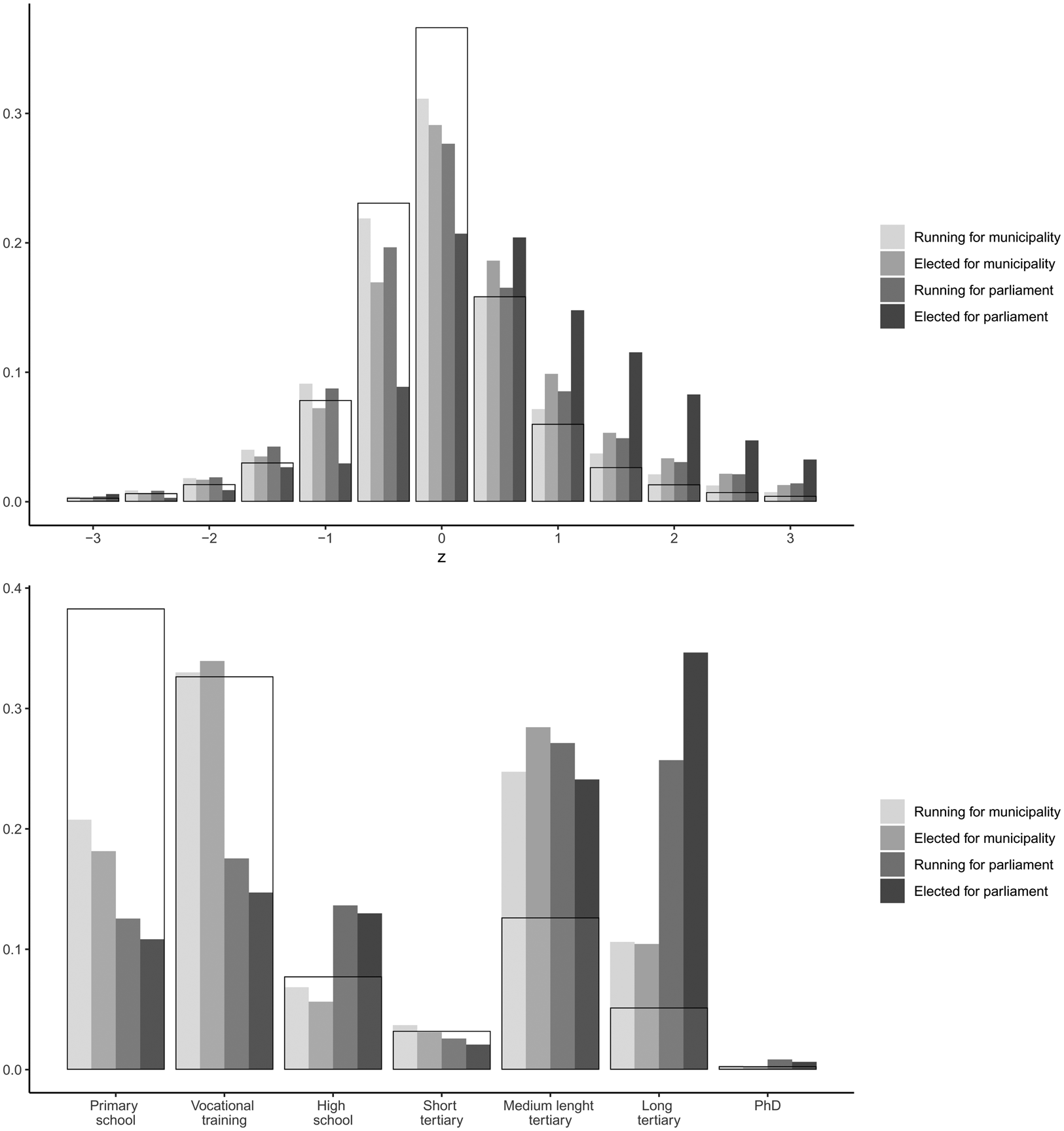
Figure 1 shows that regardless of what measure we look at, we arrive at the same conclusion. First-time elected politicians have higher earning scores and are better educated than the average population. Furthermore, this selection increases with each step up the career ladder. Candidates nominated for local government are slightly more likely to have an above average earning score, and they are more likely to hold medium-length or long tertiary educations than the population. Next, those who win a seat for local government and those nominated for national parliament score even higher on these two measures. Finally, those elected for parliament score highest on both measures. If one is willing to accept the assumption that education and earning ability in the labor markets are indicative of general ability, our results show that politicians do indeed score high on ability.Footnote 12
In the online Appendix (Section 1.2), we include graphs for differences in earning scores by election. These show that election winners always have statistically significantly higher income scores, while this is also true for those who run for local government office in three out of five elections and for those who run for national office in six out of seven elections. Those who win elections also have higher earnings scores than those who run for election. The online Appendix also include the mean earning scores for the different groups (in Table S.1). Our results turn out to be comparable in size to the results from Dal Bó et al. (Reference Dal Bó, Finan, Folke, Persson and Rickne2017). For example, in our study politicians elected for municipality or parliament have mean z-scores of 0.31 and 1.04, respectively. The corresponding results from Dal Bó et al. (Reference Dal Bó, Finan, Folke, Persson and Rickne2017) are z-scores of 0.55 for politicians elected for municipalities and 1.33 for politicians elected for parliament.
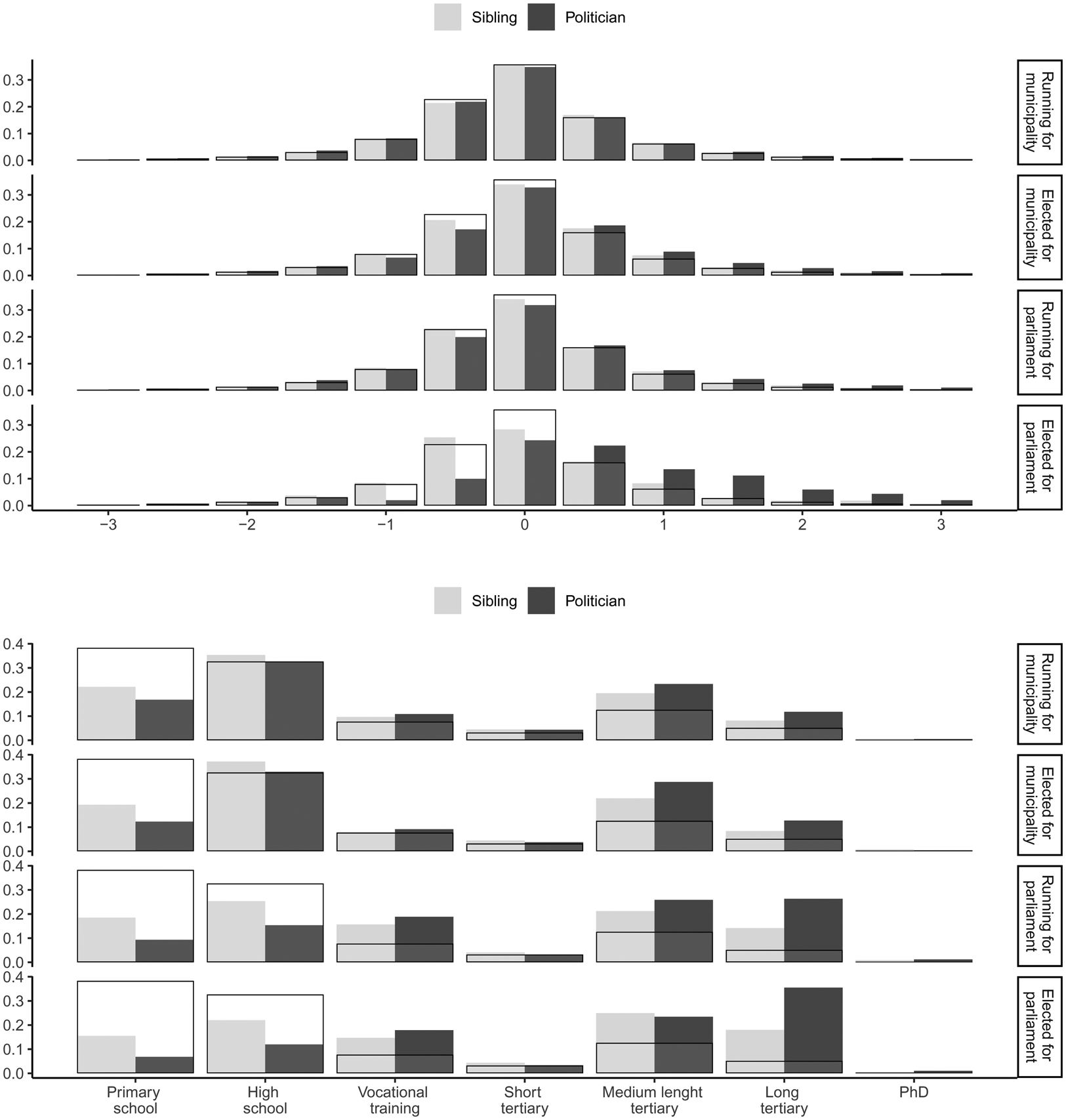
The selection that we see in Figure 1 could be due to politicians coming from socioeconomic stronger backgrounds. To explore if this explains the entire difference between politicians and the population, we compare politicians to their non-politician full siblings in Figure 2. If politicians are only better educated and better income earners due to their family background, there should be no selection when we compare them to their non-politician siblings. However, this is not the case. First-time elected politicians are more likely to have an above average income score compared to their non-politician siblings, and they are better educated. As we also saw in the comparison with the population, this selection is stronger as we move up the career ladder. The selection is weakest among those nominated for local government and strongest among those elected for national parliament.
Selection of politicians compared to siblings. The top panel shows the distribution on the z-scores from the earnings scores for the different politician groups compared to the population (transparent bars) and their siblings. We average over all elections starting in 1994 for the national elections and 1997 for the local elections. We start at the second election in our data in order to be able to remove candidates elected in an earlier term. To avoid that some very large residuals have a disproportional impact on the results, we remove the top and bottom 0.1 percent of the distribution on this variable. For the analyses, we rescale the ability measure to be centered at zero with a standard deviation of one. The bottom panel compares the distribution of politicians’ educational background to that of the population (transparent bars) and their siblings.
In the online Appendix, we compare the mean differences of the earning scores between siblings for each election. When looking at all candidates, we find that candidates at the local level generally do not have earning scores that are statistically significantly higher than their siblings, while candidates at the national level have significantly higher earning than their siblings in three out of seven national elections. However, when we look at the candidates winning office, the differences between these candidates and their siblings are generally statistically significant.
Combining the insights from Figures 1 and 2, we can see that first-time elected politicians score higher on ability, whether measured by formal education or the earnings score, than the population. We cannot explain away this finding by politicians being elected from the higher ranks of society, since the politicians are also a select group when compared to their siblings. These results show that Denmark can be characterized as a meritocracy, since merits and not only background matter.
To drive home the point that merits matter, Figure 3 compares the income distribution of politicians to that of their siblings. In the figure, we show what income percentile politicians fall in compared to their siblings. For both politicians and siblings, we place them in income percentiles relative to their gender and birth year. If politicians are selected based on elitism, their siblings should benefit from the same elitism and have higher incomes, too. Yet, the siblings are fairly evenly distributed across the income distribution, especially the siblings of local government politicians. In comparison, politicians tend to be high-income earners; especially politicians at the national level. To ensure that these results are not skewed by politicians’ returns to office, Figure 3 is based on average income in the three years leading up to the first election in which the politician ran for local or national office in our time period of investigation. We therefore also exclude data from municipal elections in 1993 and national elections in 1990, as we cannot observe whether the politicians ran in the election immediately preceding these elections.
Politicians’ income compared to that of their siblings. The figure compares the income distribution of politicians and siblings relative to their gender and birth year. Each bar represent five percentiles. The dashed lines are the population distributions, which are by definition distributed evenly across the percentile distributions. The figure is based on average income in the three years leading up to the first time the politician ran for local or national office during the time period under investigation. We start at the second election in our data in order to be able to remove candidates running in an earlier term. For each election in our time series, we then exclude anyone who ran in the same type of election in an earlier year.
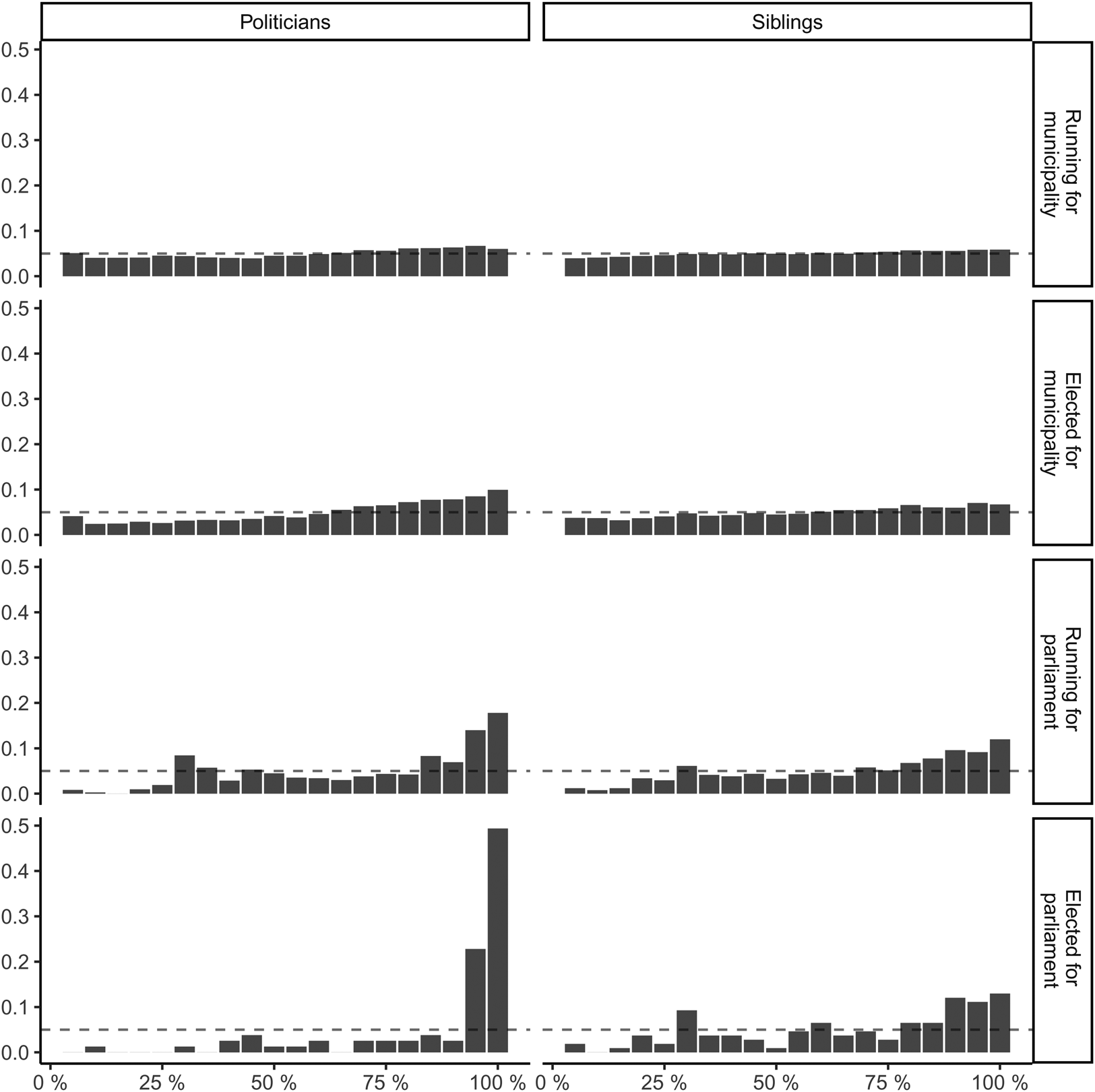
The key point in Figure 3 is that politicians’ siblings are only mildly skewed relative to the population. Had the success of politicians largely been a consequence of elitism, their siblings should have benefited from that elitism too, and it should have skewed their incomes toward the high end of the income distribution. The figure conveys that this is only the case to a limited extent. The siblings of politicians are only slightly more likely to have high incomes, especially at the local level. At the national level, it is more nuanced as more siblings are in the higher end of the income distribution. Still, low and especially middle incomes remain fairly common among siblings of those running for and elected to national office.
4.2 Selection from economically diverse backgrounds
Based on the section above, we can conclude that Denmark is a meritocracy. But is it also inclusive? As we discussed above, we limit our focus to their economic background. To operationalize economic background, we follow Dal Bó et al. (Reference Dal Bó, Finan, Folke, Persson and Rickne2017). Specifically, we focus on where fathers were in their municipality's income distribution in 1985–1987 for men with the same birth year, long before most the elections that we study, and the first years for which we have data. We focus on the income of one of the parents instead of the politicians’ own income, because, as we just saw above, politicians are selected based on their abilities. Voters and parties thus demand the same as the labor market, and, consequently, judging the inclusivity of the political system by comparing politicians’ outcomes to those of the population is not going to be very informative. Instead, we use as a yardstick what background people come. If someone, regardless of their family background, is able to make it to the political class, we will characterize the system as inclusive. We focus on fathers’ labor market earnings, because they were the only labor market participants in many traditional households, and we limit our analysis to politicians with fathers born in 1967 or earlier to make sure that the fathers were working age in 1985–1987. We average over three years of income data to limit the impact of variability in one year.
Figure 4 shows that politicians at all levels are widely selected from the entire income distribution of fathers. This is especially the case for local politicians where there is only a weak selection of candidates and election winners from the high end of the income distribution. Even among those elected for the parliament, a large proportion grew up with fathers belonging in the bottom of the income distribution. Among those running for parliament, 13.7 percent had fathers in the lowest 20 percent and 35.8 percent were below the median of the income distribution in 1985–1987 relative to the population of men of the same age in their municipality. For those elected to parliament, 12.7 percent had fathers in the lowest 20 percent of that distribution, and 31.2 percent had fathers below the median.
Distribution of fathers’ income in 1985–1987 relative to the population. The figure compares the income distribution of the fathers of politicians in 1985–1987 relative to the population of men in their municipality by their birth year. We average over three years to limit potential influence from fluctuations in one year. Each bar represents five percentiles. The dashed lines are the population distributions, which are by definition distributed evenly across the percentile distributions.
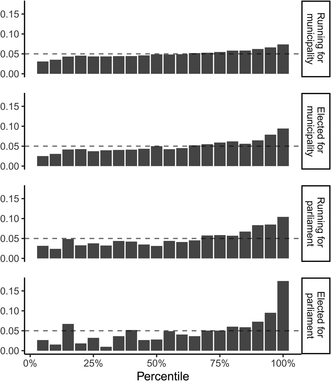
To be clear, the results in Figure 4 show that there is a considerable share of politicians at all levels that come from humble backgrounds. However, they also show that there is an over representation of politicians with well-off parents. This is most pronounced among those elected for national office, where 17.5 percent of the fathers were in the top 5 percent of the income distribution relative to their peers in 1985–1987 and 34.3 percent of the fathers where in the top 15 percent. We can also estimate a Gini-coefficient to assess the divergence from equal representation. The Gini would be zero if the was a perfect representation of all income percentiles and 0.95 if everyone was selected from just one five-percentile group. The highest Gini is found for those elected for parliament, at 0.34. For those who run for office at the local level, it is only 0.11. For comparison, the Gini for overall income inequality in Denmark, which is among one of the most egalitarian OECD-countries, has been around 0.25–0.27 in the last decade. The corresponding income Gini for, e.g., USA is 0.38–0.40 (OECD, 2023).
Another way to assess the parity of the distributions is to study how diverse politicians are on our measure of economic background compared to people of different levels of education and to the population. In Figure 5, we show the mean of the income percentile that the fathers of politicians were in from 1985 to 1987 relatively to men of the same age as them living in the same municipality in those years. For a baseline we include people with a bachelor's degree or more, a master's degree or more, and with a PhD. For the educational groups we limit the sample in each year to 48 year olds at the local level and to 45 year olds at the national level. We choose these age groups, because they correspond to the average age among politicians on those levels.
Mean of fathers’ income percentile in 1985–1987. The figure shows averages of the fathers’ place in the income distribution in 1985–1987 relative to the population of men in their municipality in 1986 by their birth year with 95 percent (CIs) for candidates including electees and those elected for office in each local and national election. The dashed lines are at the 50th percentile, which is where the average father in the population falls. In each election year, local council politicians are compared to the population of 48 year olds with a BA or higher, an MA or higher, or a PhD. National politicians are compared to 45 year olds with these educational backgrounds. These age groups are selected because they equal the average age of politicians at those levels. People with a PhD are a subset of people with an MA or more, which is a subset of people with a BA or more. PhDs are omitted from elections prior to 1998, because there are too few PhDs for whom we observe the father's income in 1985–1987.
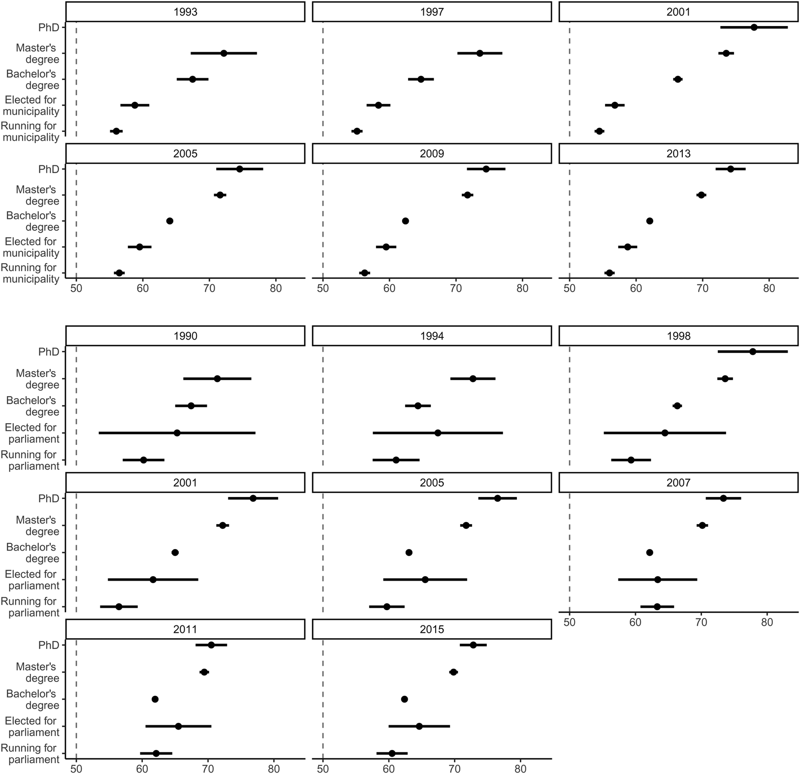
Figure 5 confirms that politicians had fathers who had higher incomes on average than their peers in 1985–1987. The selection is more pronounced on the national level, and it is stronger for those who win a seat than it is for those who merely run for office. However, as a score of 50 would imply no selection, the deviation is relatively small. Furthermore, when we compare them to groups with different levels of education, local council politicians are consistently less skewed than even those with only a bachelor's degree or more. Even politicians at the national level are only about as skewed as those of similar age with a bachelor's degree or more.
Characterizing the system as fully inclusive where everyone, regardless of their background, is equally likely to run for office and win would be a stretch. Still, the fairly dispersed distribution across parental background shows that Denmark, like Sweden, gives the opportunity regardless of starting point to enter the political class. At the highest level, of those who become elected for office, 15.9 percent have fathers in the lowest quartile of the income distribution in 1985–1987. As 17.5 percent of those elected for national office had fathers in the top 5 percent of the income distribution in 1985–1987, the descriptive representation is by no means equal, but the distributions across parental incomes still show that there are ways to make it into office regardless of one's starting point.
4.3 No ability–background trade-off
Although Figure 4 shows that politicians come from economically diverse backgrounds, we did see that they were more likely to have fathers at the top of the income distribution. This was especially true among politicians elected for national parliament, the most select group based on ability. As a final replication of the results on Sweden from Dal Bó et al. (Reference Dal Bó, Finan, Folke, Persson and Rickne2017), we show that there is, however, no trade-off between ability and representation.
To study the potential trade-off, we create an index for selection on ability and selection on background for each municipality in each year. Specifically, for a measure x with K categories, we can write the index as:
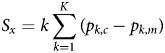
where p k,c is the proportion of candidates/council members in a given category, k, in a given municipality and p k,m is the corresponding proportion of the municipality's adult population in the same category. When candidates/council members are distributed similarly to the population, the index sums to zero. If candidates/council members are more likely to fall in higher/lower categories, the index becomes positive/negative. For our index of representation, we use the 20 categories based on fathers’ average place in the income distribution in 1985–1987. For our index of competition, we use z-scores for the earning scores in bins of half units from −3.25 to 3.25.
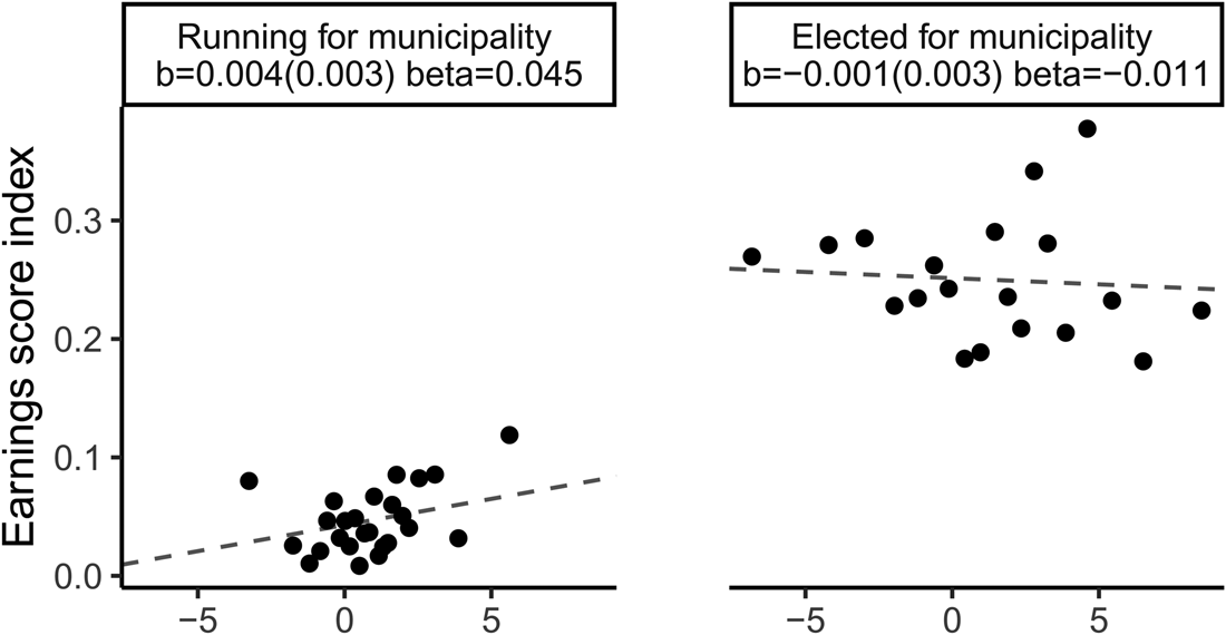
We compute each index for each municipality in every election year and plot these in Figure 6. As is evident from the plot, there is plenty of variation in both selection on ability and selection on economic background between the municipalities and election years. However, crucially, there is no apparent relationship between the two. A positive slope would indicate an ability–background trade-off where a lower degree of representation (a positive score on the selection index) is associated with a higher value on the ability index. However, we see that there is only a very weak relationship among those who run for office: a 1σ increase in the representation index is associated with a 0.045σ increase on the ability index. Among council members, the relationship is even negative and weaker in absolute terms: a 1σ increase in the representation index is associated with a 0.011σ decrease on the ability index. The results show that once again, the results from Sweden can be translated to a Danish context. There is a remarkable absence of a trade-off between representation and ability.
Representation–ability trade-off. The figure shows the relationship between the index for selection on the Y-axis and the index for representation on the X-axis. Each point represents the binned average for 50 municipality-year observations. In some early election years, there is a low number of council members for whom we know fathers’ income in 1985–1987. We include only municipality-year observations if we have five or more councilor observations.
Taken together, our results demonstrate that Denmark, like Sweden, can be characterized as an inclusive meritocracy (Dal Bó et al., Reference Dal Bó, Finan, Folke, Persson and Rickne2017). In itself this conceptual replication is important, as findings from one study should be replicated (Munafò et al., Reference Munafò, Nosek, Bishop, Button, Chambers, Du Sert, Simonsohn, Wagenmakers, Ware and Ioannidis2017; Camerer et al., Reference Camerer, Dreber, Holzmeister, Ho, Huber, Johannesson, Kirchler, Nave, Nosek, Pfeiffer, Altmejd, Buttrick, Chan, Chen, Forsell, Gampa, Heikensten, Hummer, Imai, Isaksson, Manfredi, Rose, Wagenmakers and Wu2018). However, one important characteristic that applies to both the original results and our replication is that they are all purely descriptive. For the remainder of our empirical analysis, we turn our attention to whether changing the political system can make a system more or less meritocratic or more or less inclusive. To study this, we utilize the Danish structural reform of 2007.
5. No effects of changing the political landscape
As described above, the reform of Danish municipalities implemented in 2007 dramatically changed the number of Danish municipalities. Of the 271 municipalities in existence before the reform, 239 were merged into 66 while the remaining 32 municipalities were left unchanged. The reform dramatically decreased the number of candidates and councilors, from around 17,000 candidates in the pre-reform years to around 9,000 in 2009 and 2013. In 2005, it was somewhere in between with 11,407 candidates. Likewise, the number of councilors dropped dramatically from around 4,700 to roughly 2,500. The effects of this rather dramatic reform have been investigated in several previous studies, which have looked at effects on, e.g., administrative savings (Blom-Hansen et al., Reference Blom-Hansen, Houlberg, Serritzlew and Treisman2016), voters’ political efficacy (Lassen and Serritzlew, Reference Lassen and Serritzlew2011), and turnout (Bhatti and Hansen, Reference Bhatti and Hansen2019). In this section, we will ask whether the increased competition made politicians more select on ability, made them less representative, or had an impact on the ability–background trade-off.
5.1 Does increased competition lead to increased ability?
To study the reform effect on politicians’ ability, we run a DiD model for two elections, the last before the reform and the first after. The model is of the form:

where Y i,t is the outcome of interest for politician i, in election, t, T j[i] is the treatment, i.e., being in a merged municipality, t i,t is a post-reform indicator, and α j[i] are municipality fixed effects for the post-reform structure. Finally, $\epsilon _{i, t}$ is an error term, which we cluster at the municipality level. τ DiD is the quantity of interest as it measures the treatment effect of the reform.Footnote 13 The election in 2001 took place in the old municipalities. Elections in 2005 were for the future 98 municipalities, although the reform was not implemented before 2007. We skip the 2005 election and compare 2009 outcomes to 2001. As we saw above, the number of candidates did not fully settle to a new level in 2005. By moving to 2009, we make sure that the effect of the reform on the number of candidates was fully felt.
Before estimating the effect, we plot in Figure 7 the average of the income-based ability measure with sibling fixed effects for candidates and election winners in amalgamated and continuing municipalities for each election except for 2005 compared to 2001. The black points are for the municipalities affected by the reform, whereas the gray points are for the continuing municipalities. We include sibling fixed effects, because without these the parallel trends assumption does not seem to hold. In the online Appendix, we present a plot without sibling fixed effects. Looking at the pre-reform years for selection compared to siblings, we see no clear violation of the parallel trends assumption.
Selection on ability (mincer measure) with sibling fixed effects. The figure shows the average difference relative to 2001 on the ability measure based on income for candidates for city council and election winners for every election year except for 2005 in the data with 95 percent CIs. We omit the 2005 election, because it was the election that took place when the reform was known but not implemented. The plot is split by whether the municipality was affected by the reform (amalgamated) or not (continuing). The population average for fathers is zero, so values above zero indicate that there is some selection on ability. The dashed vertical line signifies when the reform was known.
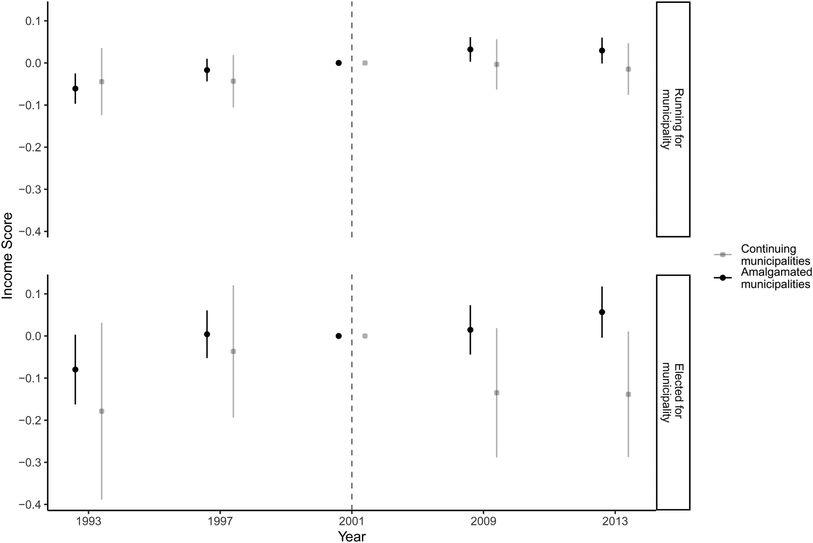
Table 1 presents the DiD between 2001 and 2009 for candidates running for local offices and the subset that wins. For each outcome we estimate a model with and without sibling fixed effects. As noted, we prefer the specifications with sibling fixed effects as we doubt the parallel trends assumption holds without. In our preferred specification, we have fewer politicians, because we can only include politicians for whom we could identify a sibling.
Effect of the reform on ability for candidates running for office
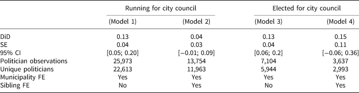
Notes: The table includes the DiD estimates obtained when comparing the difference for selection based on the ability measured using income residuals between candidates/election winners in 2009 post-reform amalgamated municipalities to post-reform continuing municipalities vis-à-vis the differences in 2001 pre-reform municipalities. Models (2) and (4) include sibling fixed effects. All models include post-reform municipality fixed effects. Standard errors clustered by the municipality in parenthesis.
The point estimates for the candidate pool running for office is 0.04 in our preferred specification with a 95 percent confidence interval (CI) of [−0.01; 0.09]. Since the outcome variable is normalized, the estimate is the change in standard deviations. For the elected candidates, the point estimates are generally larger at 0.15 standard deviations in our preferred specification with a 95 percent CI of [−0.06; 0.36]. While the point estimates are positive, both of the CIs include zero. In our alternative specification without sibling fixed effects, we also have positive point estimates both of which marginally exclude zero. However, we remind the reader that the parallel trends assumption was potentially violated in this case, and this was in a direction that could bias the DiD estimates upward and leave them entirely spurious. In an unpublished manuscript, Barfort et al. (Reference Barfort, Harmon, Lassen and Serritzlew2015) do find an effect of the reform on selection on ability using a design that resembles ours. However, when using our preferred specification, we find that the effect is not statistically significant.
5.2 Does increased competition lead to decreased representation?
Although we characterized the Danish system as inclusive, we did see some selection on the income of fathers prior to the studied time period. This was especially the case among the most elite politicians, members of parliament, where selection on ability is strongest and competition is fiercest. When competition increases at the local level, it may reduce the economic diversity of the candidates and electees. To address this question, we run a DiD model similar to the one, we saw above for selection on ability.
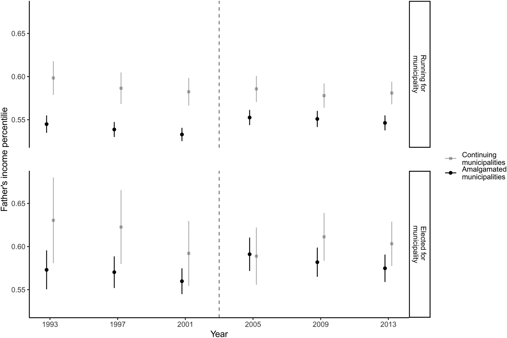
To see if the reform affected the economic diversity of the candidates/election winners, we look at the average position of fathers in the income distribution in 1985–1987. Specifically, we take as our dependent variable the income percentile, which the fathers belonged to when compared to all fathers living in the same municipality at that time and born in the same year. In Figure 8, we show the average income percentile for fathers of both candidates simply running for election and candidates winning election. The gray points are for the municipalities continuing after the reform, whereas the black points are for the amalgamated municipalities. An average of 0.5 implies that the average candidates or elected councilor is representative. Values above or below 0.5 mean that candidates or elected councilors are disproportionately from high- or low-income fathers. The average is always above 0.5, demonstrating that there is at least some consistent over-representation of better off fathers.
Average income percentile for fathers in 1985–1987. The figure shows the average income percentile that fathers belonged to in 1985–1987 relative to their municipality and birth year for candidates for city council and election winners for every election year in the data with 95 percent CIs. We average over three years to limit potential influence from fluctuations in one year. The plot is split by whether the municipality was affected by the reform (amalgamated) or not (continuing). The population average for fathers is 0.5, so values above 0.5 indicate that there is some selection on father's background. The dashed vertical line signifies when the reform was known.
From Figure 8 we also see that in every year, both candidates and city councilors in the continuing municipalities are less representative than in the municipalities affected by the reform. In Table 2, we focus on the DiD estimate for 2009 compared to 2001 to establish if the increased competition could have affected representation. We consider the amalgamation to be the treatment, and the average on the fathers’ income percentile is always above 0.5. Accordingly, a positive coefficient implies that amalgamated municipalities become less representative.
DiD result on selection on the income of fathers (1985–1987) in 2009 compared to 2001
Notes: The table includes the DiD estimates obtained when comparing the difference for selection based on the income of fathers in 1985–1987 between candidates/election winners in 2009 post-reform amalgamated municipalities to post-reform continuing municipalities vis-à-vis the differences in 2001 pre-reform municipalities. Standard errors clustered by the municipality in parenthesis.
We do not find any evidence that the reform decreased the representation based on economic background of the candidates that voters could choose from: the estimated effect is 0.014 with a 95 percent CI of [−0.017; 0.044]. As the outcome variable is the fathers’ position in the income distribution, the point estimate means the fathers of the candidates were placed 1.3 percentiles higher in the distribution in the merged municipalities following the reform. However, the CI is wide relative to the estimate. For becoming elected, we estimate the effect to be negative. The estimate is −0.033 with a 95 percent CI of [−0.099; 0.033]. As there are considerably fewer councilors than candidates, we estimate the effect on councilors with much less precision.
5.3 Does increased competition change the ability–background trade-off?
Winning a seat includes multiple steps. We can identify at least four here: (i) One has to be willing to stand for office. (ii) The party has to be willing to put one on the list. (iii) One should ideally get a good position on the list. Although the Danish system is mostly open list with a minority of parties running candidates on semi-open lists, the parties do prioritize the candidates, and those at the top of the list are far more likely to win a seat. (iv) One should win enough personal votes. Voters assign personal votes, which finally determines the faith of the parties and candidates. Our results so far suggest that the reform did not necessarily make the output of steps (i) and (ii) less inclusive nor more selective on ability, and neither did steps (iii) and (iv). Our best estimate is that the system did not become any less economically inclusive or selective on ability as a consequence of the reform.
One question still needs to be addressed: did the reform affect the trade-off between selection on ability and background? We revisit the two indices that we created for Figure 6 where we looked at the ability–background trade-off. This is to determine whether the slope of this trade-off changed as a result of the reform. If the reform induced an ability–background trade-off, we should see that the slope becomes more positive. To explore this, we estimate the DiD of the slopes before and after the reform for the continuing and amalgamated municipalities. Specifically, for municipalities, indexed by m, in 2001 and 2009 we run a model of the form:
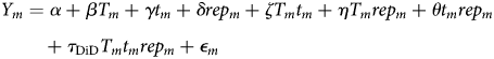
where Y m is the outcome of interest, T m is the treatment, i.e., being in a merged municipality, t m is a post-reform indicator, rep m is the representation index, and $\epsilon _{m}$ is an error term. τ DiD is the quantity of interest as it measures how much the slope for rep m changes post-reform in merged municipalities compared to the post-reform change in slope in continuing municipalities.
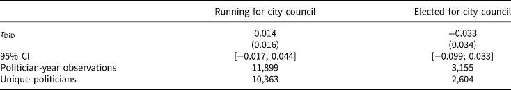
In Table 3, we present the DiD for the change in slopes between merged and continuing municipalities from 2001 to 2009.Footnote 14 We show the coefficients for both candidates and those elected for office. The coefficients for both groups are close to zero, both at 0.008 with 95 percent CIs of [−0.054; 0.069] and [−0.068; 0.085]. We also include the standardized coefficients, which may be easier to interpret. Our best estimate is that the reform meant the ability–background trade-off increased such that a 1σ increase in the representation index was associated with an additional 0.030σ ability–background trade-off in merged municipalities among candidates. Among councilors, our best estimate is that the reform meant the ability–background trade-off increased such that a 1σ increase in the representation index was associated with an additional 0.028σ ability–background trade-off in merged municipalities among candidates. Regardless of which of the two scales we interpret the coefficients on, the conclusion is the same: the reform did not substantially alter the ability–background trade-off.
DiD for ability–background trade-off in 2009 versus 2001
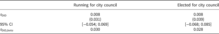
Notes: The table includes the DiD estimates for the slopes of the ability–background trade-off obtained when comparing the slope for the candidates/election winners in 2009 post-reform amalgamated municipalities to the slope of post-reform continuing municipalities vis-à-vis the differences in slopes in the 2001 pre-reform municipalities. τ DiD,beta is the standardized coefficient. Standard errors are in parenthesis.
6. Conclusion and discussion
In the beginning of the paper, we asked whether voters can have politicians who are both of high ability and from diverse backgrounds. In short, our answer is a conditional “yes,” at least in the Danish system. That is, conditional on our measures of ability and economic background: (i) Politicians are indeed positively selected both by their levels of education and by their income scores. While the average candidates have only slightly higher earning scores than the average of the voters, this difference is dwarfed by the difference between unelected and elected candidates. In other words, the relatively high level of selection among elected politicians is to a high degree a result of voters voting for the people in the pool of candidates with the highest earning scores and most education. (ii) The selection cannot be explained by background alone as politicians are selected when compared to their siblings with whom they share background. (iii) Candidates and elected politicians in our data come from all economic strata of Danish society. Although the distribution is not perfectly representative across strata, the distribution is arguably even enough to describe the political system as relatively inclusive. (iv) Our analyses suggest that there is no trade-off between selection on background and on ability. Finally, (v) a reform of the government architecture had no clear effect on the selection on ability, the selection on economic background, nor the trade-off between the two.
While we can learn a lot from these results, it is also important to be aware of some limitations. First, as we have emphasized throughout this paper, our measures of ability are far from perfect. Education and unexplained earning ability on the labor market clearly does not capture all relevant abilities or skills that may be useful as a politician. For one thing, voters may care about other aspects of politicians’ general valence, such as integrity or charisma, or performance in office (Dal Bó and Finan, Reference Dal Bó and Finan2018). Based on our data, we cannot say directly how these measures correlate with our measure of ability. The best we can do is to once again point to prior validations of the measure against policy success and test scores from military induction data on leadership ability and cognitive ability (Besley et al., Reference Besley, Folke, Persson and Rickne2017). Related to this point, it is important to note that while our analyses unequivocally shows that high-ability candidates are more likely to be elected, the electoral success of these candidates cannot necessarily be attributed to voters observing or even caring about the types of ability that we have focused on in this study. Levels of education and unexplained earning abilities may both be associated with other qualities important to the voters, and political parties may tend to promote candidates with high levels of education or earning ability in the elections campaign, thereby furthering their chances of being elected. Obvious directions for future research would be to investigate how robust the results are to other ways of measuring ability and the degree to which these measures of ability predict performance in office. For the latter question, some research seems to suggest a positive relationship between both measures of ability and performance in other contexts (Besley et al., Reference Besley, Montalvo and Reynal-Querol2011, Reference Besley, Folke, Persson and Rickne2017).
Second, it is important to emphasize that we have only studied one aspect of representation, namely economic background. While representation is relatively equal across different economic backgrounds in Denmark, the gender representation is, e.g., still far from parity, both at the national and at the local levels (Kjaer and Kosiara-Pedersen, Reference Kjaer and Kosiara-Pedersen2019). Here it is important to note that our measure of ability does take differences in labor market outcomes for men and women into account. Thus, in our analyses, the generally higher pay levels for men does not mean that men are assumed to have higher ability than women. Our study cannot tell whether a more or less equal representation of genders would affect the ability of elected politicians, but we note that a recent study finds that a more equal gender distribution may lead to increased ability among the politicians by squeezing out mediocre men (Besley et al., Reference Besley, Folke, Persson and Rickne2017). Future studies may want to incorporate other dimensions of descriptive representation, e.g., gender and ethnicity.
Finally, it is important to note that our study focuses on descriptive representation. While there is an argument that descriptive representation can also impact substantive representation, i.e., the extent to which voters’ political interests are represented (Mansbridge, Reference Mansbridge1999; Carnes, Reference Carnes2012), there are still other dimensions of representation that could be important to voters (Mansbridge, Reference Mansbridge2003; Wolkenstein and Wratil, Reference Wolkenstein and Wratil2021). In addition, it is not evident that our measure of parental background affects legislators’ behavior in office. While the link between descriptive and substantive representation is largely unexplored in the context of our study, one study from the USA questions the degree to which our measure of representation translates into substantive representation (Carnes and Sadin, Reference Carnes and Sadin2015). In sum, as was the case for our measures of ability, we only use one limited perspective to study representation.
While we acknowledge the limitation of both our measures of ability and representation, these closely follow previous research to ensure a close conceptual replication of the main results from the Swedish context.Footnote 15 We find, as in Sweden, positive selection on ability, relatively wide representation, and no ability–background trade-off. Dal Bó et al. (Reference Dal Bó, Finan, Folke, Persson and Rickne2017) label this an inclusive meritocracy. In addition to providing a conceptual replication of their descriptive results, we also show that the Danish system was robust to a reform that exogenously increased competition. The reform was applied without affecting the selection on ability, the diversity of politicians’ economic background, nor the ability–background trade-off. In conclusion, we can label Denmark a robust, inclusive meritocracy.
Given these findings, should we expect that other democracies are also inclusive meritocracies? On the one hand, our findings demonstrate that the results from Dal Bó et al. (Reference Dal Bó, Finan, Folke, Persson and Rickne2017) are not exclusive to Sweden. While Denmark and Sweden are similar in many ways, it is worth pointing out that their electoral systems do differ on some characteristics. Notably, while Swedish politicians are elected on semi-open lists, politicians in Denmark usually run on open lists, giving the voters more say in choosing which politicians are elected from a given party. This does suggest that an inclusive meritocracy does not depend entirely on parties choosing the right candidates, voters also seem to pick out the politicians with high abilities and diverse economic background (although, as previously noted, high-ability politicians may be promoted by their party even in open-list elections). Further, Denmark also differs from Sweden in having far less municipal politicians than Sweden, raising the bar for being elected as a politician. Here, the findings from Denmark suggest that more competition for political seats are not necessarily detrimental to descriptive representation.
On the other, Sweden and Denmark still share many characteristics. Both countries have, e.g., political systems with relatively strong member-based parties and proportional voting systems (Hansen and Kosiara-Pedersen, Reference Hansen and Kosiara-Pedersen2017). In addition, both countries are comparatively rich welfare states with publicly funded education at all levels and comprehensive social security systems (Kuhnle and Alestalo, Reference Kuhnle and Alestalo2017). All of these characteristics may very well play a role in the formation of inclusive meritocracies, and an important direction for future studies could be to replicate the finding from Dal Bó et al. (Reference Dal Bó, Finan, Folke, Persson and Rickne2017) and our study in countries without some of these characteristics.
Supplementary material
The supplementary material for this article can be found at https://doi.org/10.1017/psrm.2024.12. To obtain replication material for this article, https://doi.org/10.7910/DVN/H69OCL
Acknowledgments
We are grateful for comments and suggestions on earlier versions of this paper from Jon Fiva, Lene Holm Pedersen, participants, and discussants at the 2019 MPSA Conference, the 2019 EPSA Conference, the 2019 APSA Conference, the Danish Political Science Association's Yearly Meeting 2019 as well as participants at a presentations at the London School of Economics, University of Uppsala, University of Copenhagen, Copenhagen Business School, and The Danish Center for Social Science Research (VIVE). The data used in this study are stored on secure servers at Statistics Denmark, and all analyses were conducted on these servers. Due to security and privacy concerns, it is illegal to make these data publicly available. Danish research environments can be granted authorization to access the data, and foreign researchers can, under some circumstances, get access to data through an affiliation with a Danish authorized research environment.
Financial support
The authors have received support from the Danish Council for Independent Research — Social Sciences, Grant No. DFF—6109-00052.
Competing interests
None.


 Open access