4.1 The historical data

We obtained the hourly average wind speed at the Bergen station in the period of 2017–2021 from the German Weather Service.Footnote ² The Bergen station is located in Niedersachsen, the state in Germany with the highest number of turbines and installed wind power capacity. We compute the daily average wind speed by taking the mean of the hourly average wind speed on the same day. Missing values are present in the hourly wind speed dataset. If the hourly values are missing for the entire day, the daily average is imputed by the mean of the daily average values on the same day but in other years with data available.

Figure 1.

Left panel – time series plot of daily average wind speed at Bergen station in 2017–2021. Right panel – day-of-year average wind speed, with a red LOWESS smoother line.

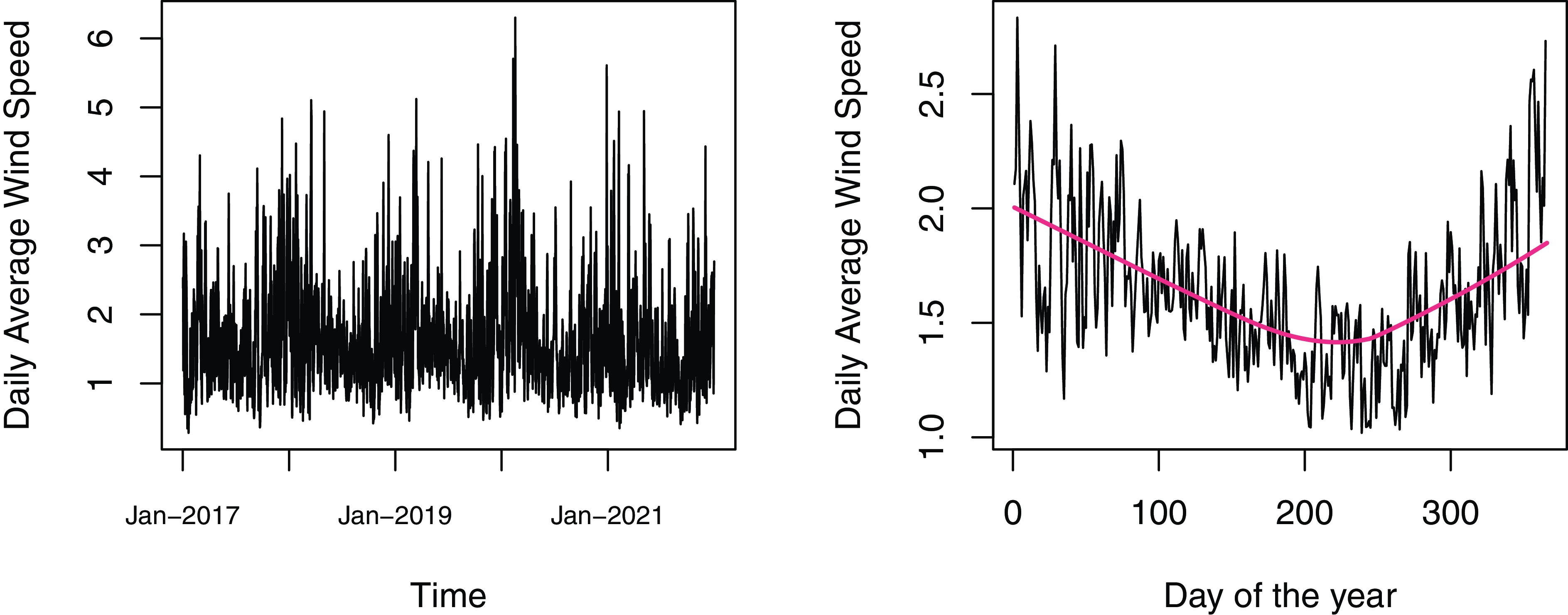
The left panel of Fig. 1 displays the time series plot of daily average wind speed at the Bergen station, with seasonal patterns clearly visible. The right panel shows the day-of-year average wind speed, calculated as the average wind speed values for the same day over the years 2017–2021, and the red line represents the corresponding LOWESS smoother. The right panel reveals higher daily average wind speed and variability in winter and lower values in summer. Table 1 provides descriptive statistics for the daily average wind speed. The notable skewness (1.39) and excess kurtosis (2.58) indicate a positively skewed and strongly non-normal wind speed distribution.

4.2 Wind speeds at turbine height

The wind speed data at the Bergen station are collected by weather transmitters located 10 m above the ground. Wind turbines, the height of which ranges from under 60 m to over 170 m, experience much stronger wind than weather transmitters. To estimate the wind speed at turbine height, we transform the wind speed obtained from weather stations using the wind profile power law, which is expressed as follows:

(3) \begin{align} W &= V \Big ( \frac{h}{s} \Big )^a, \end{align}

where $W$ is the wind speed at the turbine height $h$ , $V$ is the observed wind speed at the weather station height $s$ , and $a$ is the power law exponent. The power law exponent varies with atmospheric conditions and land features (Spera & Richards, Reference Spera and Richards1979). It is set at 1/7 in several studies (Burton et al., Reference Burton, Jenkins, Sharpe and Bossanyi2011). Burton et al. (Reference Burton, Jenkins, Sharpe and Bossanyi2011) suggest the following approximation for the power law exponent:

\begin{align*} a &= \frac{1}{\ln (h/z_0)}, \end{align*}

where $z_0$ is the roughness length representing the surface roughness. Typical roughness length for open farmland with few trees and buildings is $0.03$ m, while typical roughness length for an offshore wind farm is $0.001$ m. In the following analysis, we assume that $s=10$ , $h=90$ , and $z_0=0.03$ , which yield a power law exponent of $a=0.1249$ .

5.1 The s-AR-s-GARCH model

The pricing of wind speed derivatives requires a model that can adequately capture the features of wind speed and provide good wind speed predictions in the contract period. We capture the features of wind speed with the s-AR-s-GARCH model proposed by Gracianti et al. (Reference Gracianti, Zhou and Li2021). This model is expressed as follows:

(4) \begin{align} W_t&=\mu _t+y_t \end{align}

(5) \begin{align} y_t &= \sum _{p=1}^{P} a_p y_{t-p}+ \epsilon _t, \end{align}

(6) \begin{align} \epsilon _t &= \sigma _t z_t, \end{align}

(7) \begin{align} z_t & \sim i.i.d.(0,1), \end{align}

where $\mu _t$ is the unconditional mean of the wind speed on day $t$ , $y_t$ is the demeaned wind speed, $\epsilon _t$ is the error term, $P$ is the number of AR terms, $a_p$ is the AR coefficient, $\sigma _t$ is the volatility on day $t$ , and $z_t$ is a random variable following a distribution with zero mean and unit variance.

Table 1.

Statistics of the daily average wind speed at the Bergen station in 2017–2021

Seasonality in daily average wind speed and variance of daily average wind speed is incorporated into the model by including the Fourier series in the dynamics of $\mu _t$ and $\sigma _t$ . Volatility clustering is captured by a GARCH $(U,V)$ model for $\sigma _t$ . Mathematically, $\mu _t$ and $\sigma _t$ are further modeled as follows:

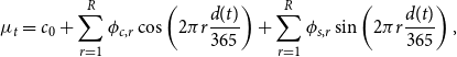(8) \begin{align} \mu _t &= c_0 + \sum _{r=1}^{R} \phi _{c,r} \cos \left (2\pi r\frac{d(t)}{365}\right )+ \sum _{r=1}^{R} \phi _{s,r} \sin \left (2\pi r\frac{d(t)}{365}\right ), \end{align}

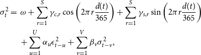(9) \begin{align} \nonumber \sigma _t^2 &= \; \omega +\sum _{r=1}^{S} \gamma _{c,r} \cos \left (2\pi r\frac{d(t)}{365}\right )+ \sum _{r=1}^{S} \gamma _{s,r} \sin \left (2\pi r\frac{d(t)}{365}\right ) \\ &\quad \,+\sum _{u=1}^U\alpha _u \epsilon _{t-u} ^2 + \sum _{v=1}^V\beta _v \sigma _{t-v}^2, \end{align}

where $R$ and $S$ represent the numbers of terms summed in the Fourier series, and $d(t)$ denotes the day of the year and cycles through $1,2,\ldots,365$ .

Gracianti et al. (Reference Gracianti, Zhou and Li2021) provide an in-depth discussion of the motivation of this model based on the study of the daily wind speed at various German weather stations. Similar models have also been considered in Taylor et al. (Reference Taylor, McSharry and Buizza2009). To avoid repetition, we summarize the key arguments for this model presented in Gracianti et al. (Reference Gracianti, Zhou and Li2021). As observed in Fig. 1, seasonality presents in both the mean and variance of wind speed. Therefore, the Fourier series is used in both mean and volatility models to capture seasonality. The AR structure is used to incorporate cyclical effects, and the suitability of an AR structure can be verified by examining the ACF and PACF plots of deseasonalized wind speeds. Volatility clustering is found to be significant upon checking the autocorrelation of squared residuals obtained from fitting an AR model to deseasonalized wind speeds. Overall, the s-AR-s-GARCH model demonstrates reasonable goodness of fit and out-of-sample forecasts.

The values of $P$ , $R$ , $S$ , $U$ , and $V$ are selected to minimize the Akaike information criterion (AIC). The considered value ranges are as follows: $P=1,\ldots,5$ , $R=1,2$ , $S=1,2$ , $U=1,2$ , and $V=1,2$ . Gracianti et al. (Reference Gracianti, Zhou and Li2021) examined the ACF and PACF plots for the wind speeds at various stations in Germany and found that a maximum of five AR lags is sufficient for most stations. Fourier series with one or two terms have been commonly employed to model seasonality in temperature and wind speed due to its parsimony (Campbell & Diebold, Reference Campbell and Diebold2005; Taylor et al., Reference Taylor, McSharry and Buizza2009; Espen & Jurate, Reference Espen and Jurate2012). They have been shown to be sufficient in removing seasonal fluctuations in their wind speed observations. Consequently, we allow the number of Fourier terms, $R$ and $S$ , to take values of 1 or 2. While the GARCH(1,1) model is often sufficient for capturing the volatility dynamics in wind speed data (Taylor et al., Reference Taylor, McSharry and Buizza2009; Gracianti et al., Reference Gracianti, Zhou and Li2021), some cases call for a more elaborate GARCH(2,2) structure (Tol, Reference Tol1997). As a result, ARCH and GARCH orders, $U$ and $V$ , are assumed to take a value of 1 or 2. We further discuss the model estimation and order selection in section 5.2.

5.2 Quasi-maximum likelihood estimation and order selection

Campbell & Diebold (Reference Campbell and Diebold2005) estimate a similar time series model for daily average temperature using the quasi-maximum likelihood (QML) estimation proposed by Bollerslev & Wooldridge (Reference Bollerslev and Wooldridge1992). The QML estimation assumes normal distribution and thus maximizes normal log-likelihood. Bollerslev & Wooldridge (Reference Bollerslev and Wooldridge1992) motivate the use of the QML estimation by showing that the estimators are not significantly biased when the true data follow a student’s $t$ distribution. Order selection and parameter estimation can be performed simultaneously. We use QML to estimate s-AR-s-GARCH models with different values of $P$ , $R$ , $S$ , $U$ , and $V$ , and we then select the model with the lowest AIC. The AIC is determined as follows:

\begin{align*} \begin{split} AIC &= -2 \ln (L) + 2N_p, \\ \end{split} \end{align*}

where $L$ is the maximized likelihood of the estimated model and $N_p$ is the number of parameters. Based on the maximized quasi-likelihood, the model with $P=2$ and $R=S=U=V=1$ is found to yield the lowest AIC.

The estimated parameters and corresponding standard errors for the selected model are presented in Table 2. All the estimated parameters are significant at 5% significance level, thereby verifying the presence of the identified wind speed features.

Table 2.

Estimated parameters and their standard errors for the s-AR-s-GARCH model using QML estimation

5.3 The generalized hyperbolic distribution

Bollerslev & Wooldridge (Reference Bollerslev and Wooldridge1992) suggest that the bias and variability of the QML estimator tend to increase with the degree of heteroskedasticity and leptokurtosis. Wind speed also exhibits skewness, the impact of which on the bias of the QML estimator is unclear. Therefore, it is necessary to consider both QML estimation and maximum likelihood (ML) estimation with other distributional assumptions and to investigate how the choice of distribution assumption affects parameter estimates. In addition, several researchers (Benth & Benth, Reference Benth and Benth2009; Alexandridis & Zapranis, Reference Alexandridis and Zapranis2013) assume normally distributed wind speed when pricing wind derivatives. The alternative distributional assumptions will aid us in assessing pricing errors that may arise from model misspecification.

To capture the skewness and leptokurtosis present in wind speed, we consider the generalized hyperbolic (GHYP) distribution and its two special cases – hyperbolic (HYP) distribution and normal inverse Gaussian (NIG) distribution for $z_t$ . The GHYP distribution is capable of modeling the leptokurtosis exhibited in daily stock returns as shown by Bibby & Sørensen (Reference Bibby and Sørensen2003) and Chen et al. (Reference Chen, Härdle and Jeong2008). It is a flexible distribution class that nests HYP, NIG, Student’s $t$ , variance-gamma, and normal distributions.

The probability density function (PDF) of a GHYP distribution can be expressed as follows:

(10) \begin{equation} f_{\text{GHYP}}(x;\; \lambda,\alpha,\beta,\delta,\mu ) = \frac{\gamma ^\lambda }{\sqrt{2\pi }\delta ^\lambda K_{\lambda }(\delta \gamma )} \cdot \frac{K_{\lambda -\frac{1}{2}}(\alpha \sqrt{\delta ^2 + (x-\mu )^2})}{(\sqrt{\delta ^2+(x-\mu )^2}/\alpha )^{\frac{1}{2}-\lambda }} \cdot e^{\beta (x-\mu )}, \;\; \, x \in \textbf{R}, \end{equation}

where $\alpha$ , $\beta$ , $\delta$ , and $\mu$ are the shape, skewness, scale, and location parameters, respectively, $\gamma ^2 = \alpha ^2 - \beta ^2$ , and $K_{\lambda }$ (.) is a modified Bessel function. The domain of the parameters are $\mu \in \textbf{R}$ and

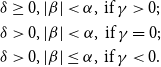\begin{align*} &\delta \geq 0, |\beta |\lt \alpha, \,\text{if}\, \gamma \gt 0;\\ &\delta \gt 0, |\beta |\lt \alpha, \,\text{if}\, \gamma =0;\\ &\delta \gt 0, |\beta |\leq \alpha, \,\text{if}\, \gamma \lt 0. \end{align*}

The moment-generating function of the GHYP distribution can be written as follows:

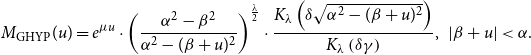(11) \begin{equation} M_{\text{GHYP}}(u) = e^{\mu u}\cdot \left ( \frac{\alpha ^2 - \beta ^2}{\alpha ^2 - (\beta + u)^2}\right )^{\frac{\lambda }{2}}\cdot \frac{K_{\lambda }\left (\delta \sqrt{\alpha ^2 - (\beta + u)^2}\right )}{K_{\lambda }\left (\delta \gamma \right )}, \;\; |\beta + u| \lt \alpha. \end{equation}

The expectation and variance of the GHYP distribution are shown below:

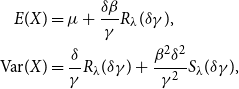\begin{align*} E(X)&=\mu + \frac{\delta \beta }{\gamma } R_{\lambda }(\delta \gamma ),\\ \text{Var}(X)&=\frac{\delta }{\gamma }R_{\lambda }(\delta \gamma ) + \frac{\beta ^2 \delta ^2}{\gamma ^2}S_{\lambda }(\delta \gamma ), \end{align*}

where $R_{\lambda }(.)$ and $S_{\lambda }(.)$ are functions defined as follows:

\begin{equation*} R_{\lambda }(u) = \frac {K_{\lambda +1}(u)}{K_{\lambda }(u)}\,\,\mbox {and}\,\, S_{\lambda }(u) = \frac {K_{\lambda +2}(u)K_{\lambda }(u)-K_{\lambda +1}^2(u)}{K_{\lambda }^2(u)}, \, \textrm{for}\, u \in \textbf {R}^+. \end{equation*}

Since $z_t$ follows a distribution with zero mean and unit variance, we impose the following constraints on $\alpha$ , $\beta$ , $\delta$ , and $\mu$ to standardize the GHYP distribution:

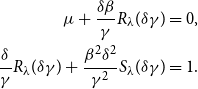\begin{align*} \mu + \frac{\delta \beta }{\gamma } R_{\lambda }(\delta \gamma ) &= 0,\\ \frac{\delta }{\gamma }R_{\lambda }(\delta \gamma ) + \frac{\beta ^2 \delta ^2}{\gamma ^2}S_{\lambda }(\delta \gamma ) &=1. \end{align*}

Therefore, only three parameters need to be estimated for the GHYP distribution.

The NIG distribution is a special case of the GHYP distribution with $\lambda =-\frac{1}{2}$ . Setting $\lambda$ to $-\frac{1}{2}$ in (10) yields the PDF of the NIG distribution:

\begin{equation*} f_{\text {NIG}}(x;\;\alpha,\beta,\delta,\mu ) = \frac {\gamma ^{-1/2}}{\sqrt {2\pi }\delta ^{-1/2} K_{{-1/2}}(\delta \gamma )} \cdot \frac {K_{-1}(\alpha \sqrt {\delta ^2 + (x-\mu )^2})}{(\sqrt {\delta ^2+(x-\mu )^2}/\alpha )} \cdot e^{\beta (x-\mu )}, \;\; \mbox {for}\, x \in \textbf{R}. \end{equation*}

The HYP distribution is a special case of the GHYP distribution with $\lambda =1$ . The PDF of the HYP distribution is given by

\begin{equation*} f_{\text {HYP}}(x;\;\alpha,\beta,\delta,\mu ) = \frac {\gamma }{\sqrt {2\pi }\delta K_{1}(\delta \gamma )} \cdot \frac {K_{\frac {1}{2}}(\alpha \sqrt {\delta ^2 + (x-\mu )^2})}{(\sqrt {\delta ^2+(x-\mu )^2}/\alpha )^{-\frac {1}{2}}} \cdot e^{\beta (x-\mu )}, \;\; \mbox {for} \, x \in \textbf {R}. \end{equation*}

5.4 Maximum likelihood estimation

We employ the maximum likelihood (ML) method to estimate s-AR-s-GARCH models with the NIG, HYP, and GHYP distributions, considering various values of $P$ , $R$ , $S$ , $U$ , and $V$ . Subsequently, we select the model yielding the lowest AIC under each distribution assumption. The parameters $\alpha$ and $\beta$ in the NIG, HYP, and GHYP distributions are not estimated directly. We estimate their transformations, $\rho =\beta/\alpha$ and $\zeta =\delta \sqrt{\alpha ^2-\beta ^2}$ , instead. We note that there is a potential identification problem in fitting the model with the GHYP distribution since a different combination of parameters $\lambda$ , $\zeta$ , and $\rho$ may lead to the same or close likelihood.

For all three distributions, the model with $P=3$ and $R=S=U=V=1$ leads to the lowest AIC. It is important to note that, under the assumption of a normal distribution, the optimal AR order $P$ is 2. This deviation in optimal AR order emphasizes how distribution assumptions can impact the model selection, which in turn affects future wind speed predictions, exemplifying model risk.

Table 3 presents the parameter estimates and their standard errors under four different distribution assumptions. The QML estimates are listed under the column “Normal” for comparative purposes. The models with the NIG, HYP, and GHYP distributions have very close parameter estimates since the NIG and HYP distributions are special cases of the GHYP distribution. All three distributions allow for skewness and excess kurtosis. Due to the different values of $\lambda$ used for the three distributions, the estimates for $\rho$ and $\xi$ change with the assumed distribution.

Table 3.

Parameter estimates for the s-AR-s-GARCH model assuming various distributions

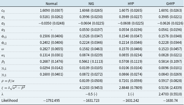
Let us compare the parameter estimates obtained under the normal and HYP assumptions. Despite differing AR orders under normal and HYP assumptions, parameter estimates remain comparable due to the utilization of the same model structure. Among the five common parameters – $c_0$ , $a_1$ , $a_2$ , $\phi _{s,1}$ , and $\phi _{c,1}$ – used for the conditional mean, only the AR coefficients $a_1$ and $a_2$ exhibit a significant difference under the two assumptions. In our model, the AR coefficients quantify how past shocks influence the current value, while the constant $c_0$ and the Fourier series coefficients $\phi _{s,1}$ and $\phi _{c,1}$ determine the long-term mean of wind speed. Since the estimated values for $c_0$ , $\phi _{s,1}$ , and $\phi _{c,1}$ do not display a significant difference under the two assumptions, we anticipate that the mean forecast of wind speed over the long term will not vary considerably. However, short-term forecasts may show significant differences.

The estimates for all five parameters – $\omega$ , $\alpha _1$ , $\beta _1$ , $\gamma _{s,1}$ , and $\gamma _{c,1}$ – in the conditional volatility display substantial differences under the two assumptions. Furthermore, the estimates for the shape and skewness parameters under the HYP distribution are significant, suggesting a considerable deviation from a normal distribution. Taking these observations into account, it is expected that the shapes of the distribution of future wind speeds under the two assumptions will differ significantly.

Therefore, the choice of distribution assumption impacts both the selected model and the estimates of model parameters, particularly those for volatility, indicating potentially significant model risk. We should be cautious about using the QML estimates in any study where volatility is an important consideration.

5.5 Model comparison

To compare the goodness of fit of the four estimated models, we compute their AIC values. A lower AIC indicates better goodness of fit. Table 4 summarizes the AIC values for the four estimated models. The normal distribution results in a much higher AIC than any other considered distribution, indicating that it is inadequate for the wind speed data. The HYP distribution leads to the lowest AIC, but it only outperforms the NIG and GHYP distributions marginally.

Table 4.

AIC values of the four models with different distribution assumptions

To further examine the suitability of the four distributions, we compare the kernel densities of the standardized residuals obtained from the four models in Fig. 2. All four density curves present a significant positive skewness. The kernel density curves obtained under the NIG, HYP, and GHYP distributions overlap with each other. Also, they are slightly more skewed than the density curve obtained under the normal distribution. The overall difference between the four density curves is small. Therefore, the choice of distribution assumption has little influence on the standardized residuals.

Figure 2

Kernel densities of the standardized residuals under various distribution assumptions.

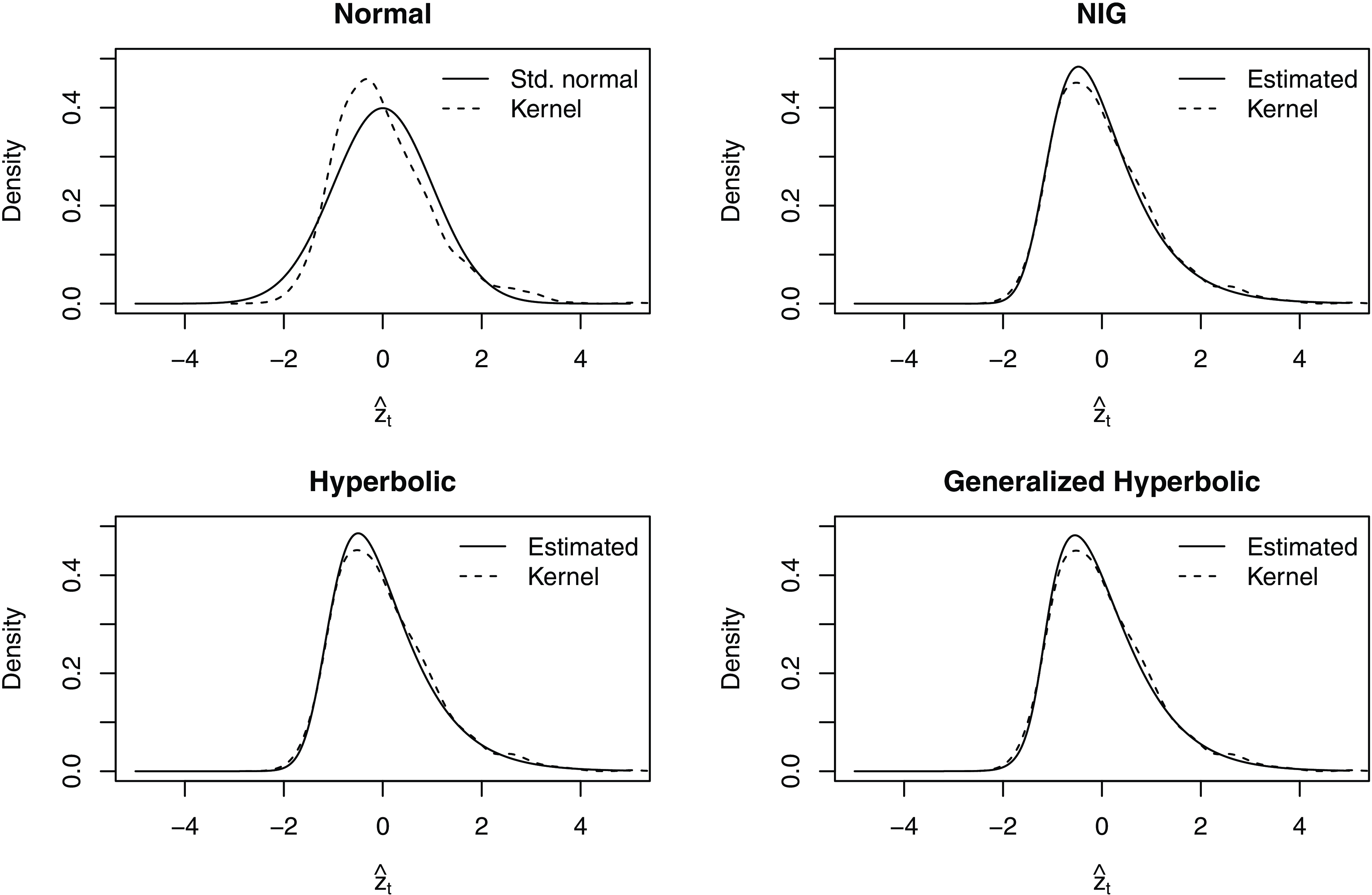
Under each distribution assumption, we also compare the theoretical or estimated density with the kernel density of the standardized residuals in Fig. 3. The solid line in the top left panel represents the theoretical density of the assumed standard normal distribution. In contrast, the dashed line represents the kernel density of the standardized residuals obtained under the normal assumption. The theoretical density is symmetric, while the kernel density is positively skewed. The kernel density also appears to have a heavier right tail and a lighter left tail than a normal distribution. The large discrepancy between the theoretical and empirical distributions of the standardized residuals indicates that the normal assumption is inappropriate. Under the NIG, HYP, and GHYP distributions, the estimated densities are calculated using the estimated distribution parameters: $\lambda$ (only estimated for the GHYP distribution), $\alpha$ , $\beta$ , $\mu$ , and $\delta$ . The differences between the estimated and kernel densities of the standardized residuals are relatively small, suggesting that the NIG, HYP, and GHYP distributions are appropriate for the wind speed data.

Figure 3

Theoretical/estimated densities and kernel densities of the standardized residuals under various distribution assumptions.

5.6 Simulating wind speed from the parametric models

Let us represent the last day in the historical wind speed data by $t=0$ . Given the choice of distribution and the corresponding estimated s-AR-s-GARCH model, we can simulate a path of future wind speed using the following procedures for $t=1,2,\ldots,t_1$ sequentially:

1. i. Calculate the conditional volatility $\sigma _t$ using (9).

2. ii. Simulate random values for $z_t$ from a standard normal distribution if normality is assumed or from the estimated distribution if one of NIG, HYP, and GHYP distributions is chosen.

3. iii. Determine the simulated wind speed value $W_t$ using (4)–(8).

4. iv. Convert the wind speed to turbine height using Equation (3).

5.7 Simulating wind speed from a semi-parametric model

The main reasons for using QML estimation are that the true distribution of the data is not required and that the normal assumption leads to an easy and efficient estimation. However, the normality assumption does not allow us to incorporate skewness and excess kurtosis in the simulation of future wind speed. Such features, which have been observed in Fig. 2, can potentially impact derivative prices significantly. To overcome this problem, we consider the semi-parametric model for wind speed proposed by Gracianti et al. (Reference Gracianti, Zhou and Li2021). A non-parametric distribution is used for $z_t$ in the semi-parametric approach, such that the skewness and leptokurtosis can be retained in the simulated wind speed.

Figure 4

Kernel densities of simulated wind speed at turbine height on 03/31/2022 under various distribution assumptions.

The standardized residuals are first obtained from the QML estimation. Sequential procedures similar to those described in section 5.6 are used for simulating future wind speed, but with the simulated normal random values replaced by the bootstrapped samples from the standardized residuals. The simulated values for volatility and wind speed are then calculated using the QML estimates. More specifically, the simulation procedures are summarized as follows:

1. i. Obtain the standardized residuals from the QML estimation of the s-AR-s-GARCH model.

2. ii. Draw a random sample from the standardized residuals and use it as the simulated values for  ${z}_t$ .

3. iii. Calculate the volatility $\sigma _t$ using Equation (9) and the QML estimates.

4. iv. Determine the simulated wind speed value $W_t$ using Equations (4)–(8) and the QML estimates.

5. v. Convert the wind speed to turbine height using Equation (3).

A similar semi-parametric approach is adopted by Badescu & Kulperger (Reference Badescu and Kulperger2008), who approximate the true distribution of stock returns with a non-parametric density estimator. They find that their proposed semi-parametric approach yields relatively accurate option prices. Although the semi-parametric approach retains the non-normality in the simulation of future wind speed, it still suffers from biased estimates due to the use of the QML estimator. We investigate the extent to which the semi-parametric model can alleviate the impact of model risk on wind derivative pricing.

5.8 Simulated future wind speed

Fig. 4 plots the kernel densities of the simulated wind speed on 03/31/2022 at the turbine height using models with different distribution assumptions. The vertical lines represent corresponding mean values. The density curves and mean values obtained under the NIG, HYP, and GHYP assumptions almost overlap in the right panel. This observation is not surprising since the three assumptions yield very similar parameter estimates. In the left panel, the density curves under the bootstrap, normal, and HYP assumptions have notably different spreads, with the largest spread under the normal assumption and the lowest spread under the HYP assumption. While similar tail shapes are observed under the bootstrap and HYP assumptions, the normal assumption leads to a lighter right tail and a heavier left tail than the other assumptions. The mean values under the normal and HYP assumptions are very close, while the mean value under the bootstrap method is slightly higher. These observations align with the findings from the comparison of estimated model parameters. The simulated wind speed for 03/31/2022 represents a 90-day-ahead prediction, thereby indicating a long-term projection. Based on the analysis of model estimates, it is anticipated that the mean forecasts for the long-term will be similar under the two distribution assumptions, while the shapes of the distributions exhibit substantial differences.

The observations from Fig. 4 suggest that if the wind derivative prices are largely determined by the mean values of future wind speed, the pricing error due to the normal assumption can be small and the semi-parametric approach may not provide much benefit. However, if the derivative prices are related to a specific portion of the density curve, such as the tails, the pricing error arising from an inappropriate distribution assumption can be large, and simulating from the semi-parametric model may reduce the error to some extent.

Since the NIG, HYP, and GHYP distributions result in very similar parameter estimates and simulated future wind speed, we only consider the HYP distribution, which leads to the lowest AIC in model fitting, in the following analysis.

6.1 Risk-neutral pricing and the Esscher transform

The wind speed dynamics described in section 5 are specified under the real-world measure. The derivative price can be calculated as the expected discounted derivative payoff under the real-world measure. Since investors demand risk premiums for bearing the uncertainty, the discount rate needs to be adjusted for individual risk preferences; these are difficult to quantify. Risk-neutral pricing adjusts the probabilities of future outcomes such that all assets have the same expected rate of return, the risk-free rate, under the new probability measure. Such a probability measure is called the risk-neutral measure. The price of a derivative is its expected discounted payoff in the risk-neutral world, with the discount rate set to the risk-free rate.

In a complete market where derivative payoffs can be replicated by a portfolio of existing assets, the risk-neutral measure is unique. However, the wind derivative market is incomplete partly because the wind speed is not directly tradable and partly because the sophisticated dynamics of wind speed imply market incompleteness. The incompleteness of the wind derivative market leads to infinite risk-neutral measures, each of which produces a risk-neutral price.

The Esscher transform is a technique used to obtain a risk-neutral measure. The use of the Esscher transform has been justified by several researchers. Gerber & Shiu (Reference Gerber and Shiu1994) show that Esscher transform maximizes the expected power utility function of a representative economic agent. Chan (Reference Chan1999) demonstrates that the minimum relative entropy measure can be constructed from the Esscher transform. Wang (Reference Wang2003) derives the Esscher transform from the Bühlmann’s equilibrium pricing model under some assumptions on the aggregate risk. Kijima (Reference Kijima2006) proves that multivariate Esscher and Wang transforms coincide when the underlying risks are normally distributed. Since the introduction of the Esscher transform by the seminal work of Gerber & Shiu (Reference Gerber and Shiu1994), the Esscher transform has been extensively applied in derivative pricing.

6.2 Conditional Esscher transform

There have been several applications of Esscher transform in pricing weather derivatives, including temperature derivatives (Ahčan, Reference Ahčan2012), rainfall futures (Cabrera et al., Reference Cabrera, Odening and Ritter2013), and wind power futures (Benth & Pircalabu, Reference Benth and Pircalabu2018). The Esscher transform is well-suited for applications that assume deterministic volatility in weather variables. However, our wind speed model incorporates a GARCH volatility structure, necessitating the use of the more versatile conditional Esscher transform. This was proposed by Bühlmann et al. (Reference Bühlmann, Delbaen, Embrechts and Shiryaev1996) as a generalization of the Esscher transform to accommodate a broader range of stochastic processes.

Consider a discrete-time economy with the time index $t = 0, 1,\ldots,T$ . Let $(\Omega,\mathcal{F},\mathcal{F}_t,P)$ be a filtered probability space, where $P$ is the real-world probability measure and the filtration $\mathcal{F}_t$ is a sequence of increasing $\sigma$ -fields of $\mathcal{F}$ representing all the market information up to time $t$ . We assume that $\mathcal{F}_0=\{0,\Omega \}$ and $\mathcal{F}_T=\mathcal{F}$ .

Let $(x_t)_{0\leq t\leq T}$ be a process adapted to the filtration $\mathcal{F}_t$ . The conditional moment-generating function of $x_t$ w.r.t. $\mathcal{F}_{t-1}$ is expressed as follows:

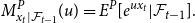\begin{equation*}M^P_{x_t|\mathcal {F}_{t-1}}(u) = E^P[e^{u x_t}|\mathcal {F}_{t-1}].\end{equation*}

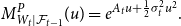
We assume that the $M^P_{x_t|\mathcal{F}_{t-1}}(u)$ exists for $0\leq t \leq T$ and $|u|\lt k$ , where $k$ is some positive real number.

Let the process $Z_t$ be defined by

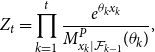\begin{equation*} Z_t = \prod _{k=1}^t \frac {e^{\theta _k x_k}}{M^P_{x_k|\mathcal {F}_{k-1}}(\theta _k)}, \end{equation*}

where $Z_0=1$ and $\theta _t$ is a $\mathcal{F}_{t-1}$ -measurable process. $\theta _t$ is also called the conditional Esscher parameter. It is easy to verify that the sequence $\{Z_t\}$ is a martingale. The conditional Esscher transform $Q$ w.r.t. $P$ of the process $x_t$ is defined as follows:

(12) \begin{equation} \frac{\text{d} Q}{\text{d}P}\Big |_{\mathcal{F}_t}= Z_t. \end{equation}

The conditional Esscher transform is very versatile and can be applied in the GARCH framework with any type of distribution as long as the moment-generating function exists.

The conditional moment-generating function of $x_t$ under $Q$ can be written as follows: (Siu et al., Reference Siu, Tong and Yang2004):

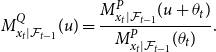(13) \begin{equation} M^{Q}_{x_t|\mathcal{F}_{t-1}}(u) = \frac{M^{P}_{x_t|\mathcal{F}_{t-1}}(u+\theta _t)}{M^{P}_{x_t|\mathcal{F}_{t-1}}(\theta _t)}. \end{equation}

Equation (13) will be used to derive the wind speed dynamics under the risk-neutral measure.

6.3 The conditional Esscher parameter

In the option pricing literature (Siu et al., Reference Siu, Tong and Yang2004; Badescu & Kulperger, Reference Badescu and Kulperger2008) where $x_t$ is the log stock return, $\theta _t$ is the unique solution to the following equation:

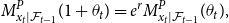\begin{equation*} M^{P}_{x_t|\mathcal {F}_{t-1}}(1+\theta _t)=e^{r}M^{P}_{x_t|\mathcal {F}_{t-1}}(\theta _t), \end{equation*}

where $r$ is the risk-free interest rate. This equation is equivalent to $E^{Q}[e^{x_t}|\mathcal{F}_{t-1}]=e^r$ , which ensures that the expected return of the stock under $Q$ is equal to the risk-free rate. However, we cannot impose this condition when $x_t$ represents wind speed since wind speed is not a tradable asset.

In this paper, we assume that the conditional Esscher parameters are time-invariant and $\theta _t=\theta$ . We examine the prices of wind speed derivatives assuming various values of $\theta$ . In future research, we plan to calibrate the conditional Esscher parameters using the observed wind power future prices and study how the parameters evolve over time.

The absolute value of $\theta _t$ can also be viewed as the market price of risk. The higher the absolute value, the more compensation investors demand for bearing the risk. The sign of $\theta _t$ is not necessarily positive. Let us consider a wind energy producer who trades wind speed derivatives to hedge the uncertainty in wind power production. To achieve an effective hedge, the producer should take a short position on the underlying wind speed index. Therefore, the producer should short the future or long the put option. Since the investors who are in long positions on the underlying index demand risk premiums, the conditional Esscher parameters should be negative such that the distribution of the wind speed index is shifted to the left with the change of measure from $P$ to $Q$ .

6.4 Wind speed dynamics under the risk-neutral measure

Under the real-world measure $P$ , the wind speed is assumed to follow the dynamics expressed in Equations (4)–(9). The mean and variance of the conditional variable $W_t|\mathcal{F}_{t-1}$ are $\mu _t+\sum _p a_p y_{t-p}$ and $\sigma _t^2$ respectively. Assuming that $z_t$ follows a parametric distribution, Normal, NIG, HYP, or GHYP, we derive the distribution of $W_t|\mathcal{F}_{t-1}$ under $Q$ and the corresponding risk-neutral wind speed dynamics.

Normal distribution

Assume that $z_t$ follows a standard normal distribution under $P$ . We have ${W}_t |\mathcal{F}_{t-1} \sim N(A_t,\sigma _t^2)$ , where $A_t=\mu _t+\sum _p a_p y_{t-p}$ . The moment-generating function of ${W}_t |\mathcal{F}_{t-1}$ under $P$ can be written as follows:

\begin{equation*}M_{{W}_t |\mathcal {F}_{t-1}}^P(u) =e^{A_t u+\frac {1}{2}\sigma _t^2 u^2}.\end{equation*}

Using Equation (13), the moment-generating function of ${W}_t |\mathcal{F}_{t-1}$ under $Q$ can be derived as follows:

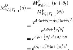\begin{align*} M^{Q}_{W_t|\mathcal{F}_{t-1}}(u) &= \frac{M^{P}_{W_t|\mathcal{F}_{t-1}}(u+\theta _t)}{M^{P}_{W_t|\mathcal{F}_{t-1}}(\theta _t)} \\ &=\frac{e^{A_t (u+\theta _t) + \frac{1}{2} \sigma _t^2 (u+\theta _t)^2}}{e^{A_t \theta _t + \frac{1}{2}\sigma _t^2 \theta _t^2}}\\ &= e^{A_t u + \frac{1}{2} \sigma _t^2 u^2 + \sigma _t^2 \theta _t u}\\ &= e^{(A_t + \sigma _t^2\theta _t )u + \frac{1}{2} \sigma _t^2 u^2}. \end{align*}

Therefore, the distribution of $W_t|\mathcal{F}_{t-1}$ under $Q$ is normal with mean $A_t + \sigma _t^2\theta _t$ and variance $\sigma _t^2$ .

Let $S_t=\sum _{r=1}^{S} \gamma _{c,r} \cos \left (2\pi \frac{d(t)}{365}\right )+ \sum _{r=1}^{S} \gamma _{s,r} \sin \left (2\pi \frac{d(t)}{365}\right )$ . The volatility dynamics under $P$ can be rewritten as follows:

\begin{equation*} \sigma _t^2 = \omega + S_t+ \alpha _1 \epsilon _{t-1} ^2 + \beta _1 \sigma _{t-1}^2. \end{equation*}

It is important to note that the distribution of $\epsilon _t|\mathcal{F}_{t-1}$ under $Q$ is normal with mean $\sigma _t^2 \theta _t$ and variance $\sigma _t^2$ . We define a new random variable $\xi _t=\epsilon _t-\sigma _t^2\theta _t$ . The distribution of $\xi _t|\mathcal{F}_{t-1}$ is normal with mean 0 and variance $\sigma _t^2$ under $Q$ . Replacing $\epsilon _t$ with $\xi _t+\sigma _t^2\theta _t$ , the dynamics of wind speed under $Q$ can be written as follows:

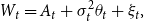(14) \begin{align} W_t&=A_t+ \sigma _t^2 \theta _t+\xi _t, \end{align}

(15) \begin{align} \sigma _t^2& = \omega +S_t+ \alpha _1 (\xi _t+ \sigma _t^2\theta _t) ^2 + \beta _1 \sigma _{t-1}^2, \end{align}

where $\xi _t|\mathcal{F}_{t-1}\sim N(0,\sigma _t^2)$ .

GHYP distribution

Assume that $z_t$ follows $\text{GHYP}(\lambda,{\alpha },{\beta },{\delta },{\mu })$ under $P$ . The conditional variable $W_t|\mathcal{F}_{t-1}$ also follows a GHYP distribution as shown below:

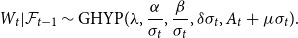\begin{equation*}W_t|\mathcal {F}_{t-1}\sim \text {GHYP}(\lambda,\frac {\alpha }{\sigma _t},\frac {\beta }{\sigma _t},{\delta }{\sigma _t},A_t+\mu \sigma _t).\end{equation*}

Using Equation (11), the moment-generating function of $W_t|\mathcal{F}_{t-1}$ under $P$ can be written as follows:

\begin{equation*}M^P_{W_t|\mathcal {F}_{t-1}}(u) = e^{(A_t+{\mu }\sigma _t) u} \cdot \Bigg ( \frac {{\alpha }^2 - {\beta }^2}{{\alpha }^2 - ({\beta } + u\sigma _t)^2}\Bigg )^{\frac {\lambda }{2}}\cdot \frac {K_{\lambda }({\delta } \sqrt {{\alpha }^2 - ({\beta } + u\sigma _t)^2})}{K_{\lambda }({\delta } \sqrt {{\alpha }^2 - {\beta }^2}) }, \;\; |{\beta } + u\sigma _t| \lt {\alpha }. \end{equation*}

Using Equation (13), the conditional moment-generating function under $Q$ can be derived as follows:

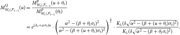\begin{align*} \begin{split} M^{Q}_{W_t|\mathcal{F}_{t-1}}(u) &= \frac{M^{P}_{W_t|\mathcal{F}_{t-1}}(u+\theta _t)}{ M^{P}_{W_t|\mathcal{F}_{t-1}}(\theta _t)} \\ &=e^{(A_t+\mu \sigma _t)u}\cdot \Bigg ( \frac{{\alpha }^2 - ({\beta } + \theta _t\sigma _t)^2}{{\alpha }^2 - ({\beta } + (u+\theta _t)\sigma _t)^2}\Bigg )^{\frac{\lambda }{2}} \cdot \frac{K_{\lambda }({\delta } \sqrt{{\alpha }^2 - ({\beta }+(u+\theta _t)\sigma _t)^2})}{K_{\lambda }({\delta } \sqrt{{\alpha }^2 - ({\beta } + \theta _t\sigma _t)^2})}. \end{split} \end{align*}

Therefore, under $Q$ , the conditional variable follows a GHYP distribution as shown below:

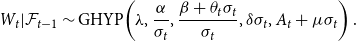\begin{equation*} W_t|\mathcal {F}_{t-1}\sim \text {GHYP}\!\left(\lambda,\frac {\alpha }{\sigma _t},\frac {{\beta }+\theta _t \sigma _t}{\sigma _t},{\delta }\sigma _t,A_t+{\mu }\sigma _t\right).\end{equation*}

We define a new random variable $\xi _t$ , which takes the following conditional distribution:

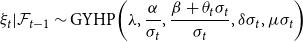\begin{equation*}\xi _t|\mathcal {F}_{t-1}\sim \text {GYHP}\!\left(\lambda,\frac {\alpha }{\sigma _t},\frac {{\beta }+\theta _t \sigma _t}{\sigma _t},{\delta }\sigma _t,{\mu }\sigma _t\right)\end{equation*}

under $Q$ . It is easy to see that $\epsilon _t|\mathcal{F}_{t-1}$ follows the same distribution with $\xi _t|\mathcal{F}_{t-1}$ under $Q$ . The dynamics of the wind speed under $Q$ can be written as follows:

(16) \begin{align} W_t&=A_t+ \xi _t, \end{align}

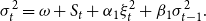(17) \begin{align} \sigma _t^2& = \omega +S_t+ \alpha _1 \xi _t ^2 + \beta _1 \sigma _{t-1}^2. \end{align}

NIG and HYP distributions

NIG and HYP are special cases of GHYP distribution. The dynamics of the wind speed under $Q$ are the same as those shown in Equations (16) and (17) with the GHYP parameter $\lambda$ set to $-1/2$ for the NIG distribution and 1 for the HYP distribution.

6.5 Pricing approaches

Under the risk-neutral measure, the price of a wind speed derivative is calculated as the expectation of derivative payoffs discounted at the risk-free rate. Therefore, the derivative price at time 0 can be written as $E^Q[e^{-rt_1}g(\text{CWSI}_{[t_0,t_1]})]$ . We consider two approaches for the expectation calculation, with one approach simulating future wind speed paths under the risk-neutral measure and the other approach under the real-world measure.

In the first approach, we simulate $N$ paths of future wind speed directly from the risk-neutral dynamics, which are defined in Equations (14) and (15) under the normal assumption and in Equations (16) and (17) under the NIG/HYP/GHYP assumption. The simulation procedures are the same as those described in section 5.6, but they use the risk-neutral wind speed dynamics. Let $\text{CWSI}^{Q}_{[t_0,t_1]}(i)$ denote the cumulative wind speed index determined under the $i$ th simulated risk-neutral path. The derivative price can be calculated as follows:

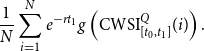(18) \begin{equation} \frac{1}{N}\sum _{i=1}^{N}e^{-rt_1} g\left (\text{CWSI}^Q_{[t_0,t_1]}(i)\right ). \end{equation}

This approach is efficient and convenient to use when the risk-neutral dynamics can be easily simulated. It is commonly used in stock option pricing (Siu et al., Reference Siu, Tong and Yang2004).

In the second approach, we simulate $N$ paths of future wind speeds from the real-world dynamics as defined in Equations (4)–(7). Let $\text{CWSI}^{P}_{[t_0,t_1]}(i)$ denote the cumulative wind speed index corresponding to the $i$ th simulated real-world path. The derivative price at time $t$ can be calculated as follows:

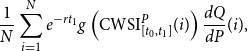(19) \begin{equation} \frac{1}{N} \sum _{i=1}^N e^{-rt_1}g\left (\text{CWSI}^P_{[t_0,t_1]}(i)\right ) \frac{dQ}{dP}(i), \end{equation}

where $\frac{dQ}{dP}(i)$ is the Radon-Nikodym derivative defined in Equation (12) with $t=t_1$ and evaluated under the $i$ th real-world path. This approach does not require the risk-neutral dynamics of $W_t$ . It is particularly useful when the risk-neutral dynamics follow a complex structure and thus cannot be simulated easily.

In section 5.7, we describe the simulation of future wind speed from a semi-parametric model, which aims to mitigate potential pricing errors arising from model misspecification. Due to the use of the bootstrap procedure, we cannot express the corresponding risk-neutral dynamics easily. Therefore, only the second pricing approach can be used with the semi-parametric model. After simulating each wind speed path under the real-world measure, we calculate the Radon-Nikodym derivative under this path. Equation (19) is used to calculate the derivative price after simulating all $N$ paths.

7.1 Simulated wind speed index values under $Q$

Benth & Pircalabu (Reference Benth and Pircalabu2018) calibrate the Esscher parameter $\theta$ by utilizing observed prices of wind power futures based on the NAREX WIDE index from 2016. Their findings reveal that the magnitude of the calibrated Esscher parameters ranges between 0 and 0.1 and decreases as the delivery period lengthens. For a three-month contract, the calibrated $\theta$ is approximately 0.6. Furthermore, Benth & Pircalabu (Reference Benth and Pircalabu2018) note that the closing price falls below the theoretical price when $\theta$ equals 0, signifying that the energy producer, who holds the short position, pays a positive risk premium. To account for this observation, the condition $\theta \leq 0$ is imposed in our pricing applications.

We select the three values for $\theta$ : 0, $-0.05$ , and $-0.1$ , to illustrate the pricing of wind speed derivatives. We simulate 10,000 wind speed paths for the period of 01/01/2022–03/31/2022 under the risk-neutral measure with $\theta$ set to 0, $-0.05$ , and $-0.1$ , respectively. We view 12/31/2021 as day 0 and assume that the derivatives are traded at $t=0$ . The wind speed index is accumulated over the period of $[t_0,t_1]$ with $t_0=1$ and $t_1=90$ .

Fig. 5 presents the density curves of the simulated $\text{CWSI}_{[t_0,t_1]}$ under various distribution assumptions and values of $\theta$ . The top panels compare the kernel densities of simulated $\text{CWSI}_{[t_0,t_1]}^{(1)}$ while the bottom panels compare those of simulated $\text{CWSI}_{[t_0,t_1]}^{(2)}$ . When $\theta =0$ , simulating under $Q$ is the same as simulating under $P$ . In the top left and bottom left panels where $\theta =0$ , we compare the density curves of three sets of index values simulated under $P$ using the normal, HYP, and non-parametric (bootstrap) distributions, respectively. The vertical lines represent the mean values corresponding to the densities. As $\theta$ becomes more negative, the density curves and their mean values shift further to the left, thereby resulting in lower future prices and higher put option prices.

Figure 5

The kernel densities of simulated $\text{CWSI}_{[t_0,t_1]}$ under various distribution assumptions and $\theta$ values, with the vertical lines representing corresponding mean values.

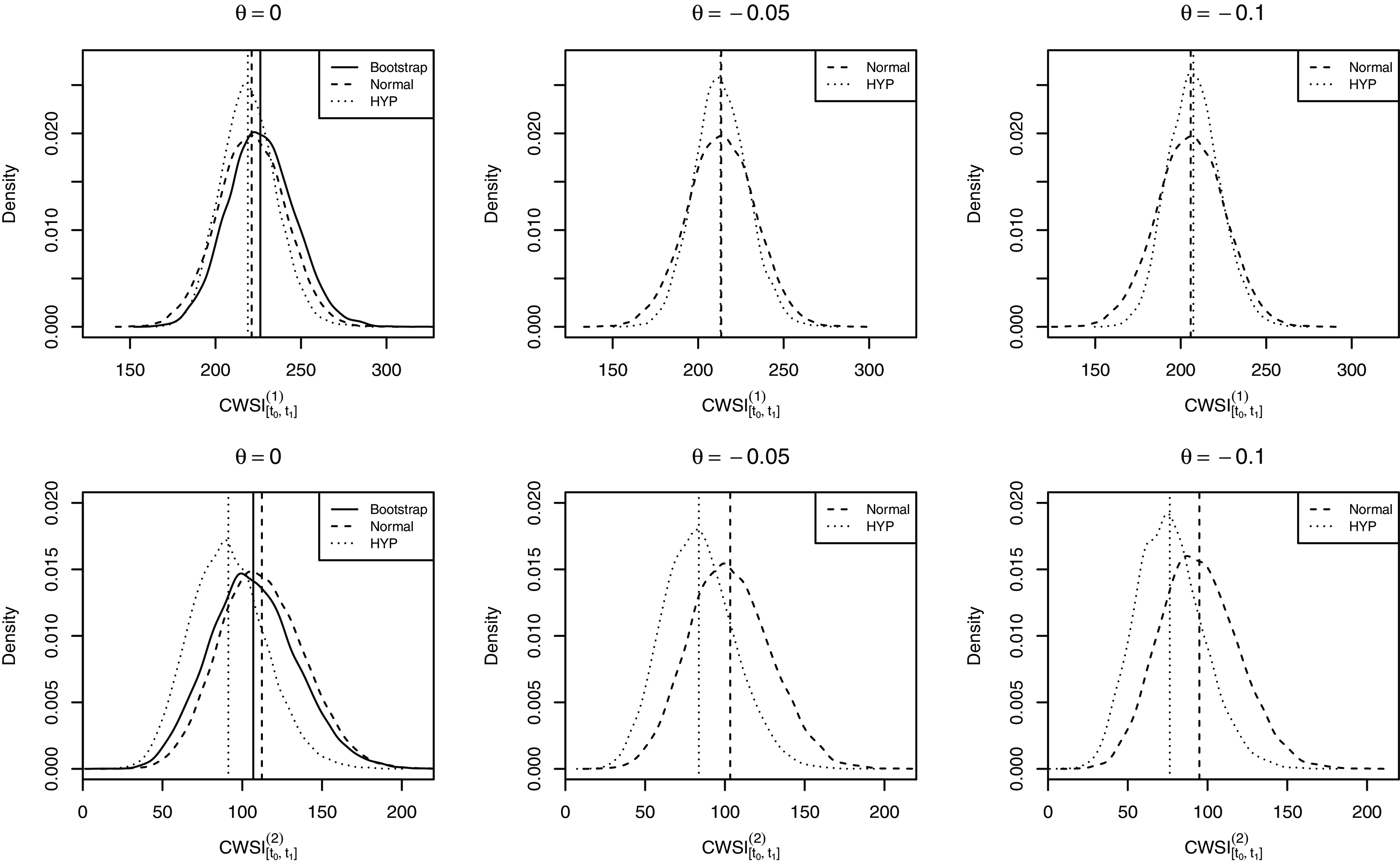
The spread of the density curve under the HYP distribution also changes with $\theta$ , while the spread under the normal distribution does not experience visible change. The change of measure in risk-neutral pricing shifts the skewness parameter of the HYP distribution by $\theta$ and subsequently changes the variance of the wind speed. As $\theta$ becomes more negative, the variance of wind speed under the HYP distribution is further decreased. On the other hand, the change of measure only shifts the mean but not the variance of the normal distribution.

The top panels show that the mean values of simulated $\text{CWSI}_{[t_0,t_1]}^{(1)}$ under the normal and HYP distributions are very close, although the variance under the HYP distribution is smaller. As shown in Fig. 4, we observed similar mean values of simulated wind speed under the normal and HYP distributions in the real world. Since $\text{CWSI}_{[t_0,t_1]}^{(1)}$ is simply the sum of wind speed values over the period of $[t_0,t_1]$ , the mean values of simulated $\text{CWSI}_{[t_0,t_1]}^{(1)}$ under the two distribution assumptions are expected to be close too. The density curve using the bootstrap approach has a similar shape to that using the normal distribution but a higher mean value. Based on these observations from the top panels, we expect the price of a future written on $\text{CWSI}_{[t_0,t_1]}^{(1)}$ not to differ significantly when the distribution is switched from normal to HYP. However, the price of an option with a certain strike price may experience a larger price difference since the tails of the density curves under the two distributions are significantly different. The semi-parametric model is not likely to reduce pricing errors arising from misspecified distribution for futures written on $\text{CWSI}_{[t_0,t_1]}^{(1)}$ .

The bottom panels demonstrate that the mean values of simulated $\text{CWSI}_{[t_0,t_1]}^{(2)}$ under the normal assumption are much higher than those under the HYP assumption. In Fig. 4, we observe that the normal distribution leads to higher densities for wind speed between 3 and 4.88 and slightly lower densities for wind speed above 4.88 in comparison to the HYP distribution. Since $\text{CWSI}_{[t_0,t_1]}^{(2)}$ only cumulates wind speed between 3 and 25 and the probability of wind speed above 4.88 is very low, the normal assumption results in significantly higher mean values for $\text{CWSI}_{[t_0,t_1]}^{(2)}$ . The density curve using the bootstrap approach has a shape similar to that using the normal distribution but a slightly lower mean value. Based on the observations made on the bottom panels, we expect large price differences for derivatives written on $\text{CWSI}_{[t_0,t_1]}^{(2)}$ under the normal and hyperbolic assumptions. The price difference between using the bootstrap and HYP assumption is expected to be smaller. Therefore, the semi-parametric model may reduce pricing errors arising from misspecified distribution by a small amount.

7.2 Pricing results

The tick size $D$ is set to 1 without loss of generality. The 25th, 50th, and 75th percentiles of the historical wind speed index values in 2012–2021 are used as the strike prices for put options. The risk-free interest rate $r$ is set at 4% per annum. Tables 5 and 6 present the prices of derivatives written on $\text{CWSI}_{[t_0,t_1]}^{(1)}$ and $\text{CWSI}_{[t_0,t_1]}^{(2)}$ respectively. In both tables, we show the prices obtained with the two proposed pricing approaches and under various choices of distributions and $\theta$ values. When $\theta =0$ , the two probability measures $P$ and $Q$ are the same, and thus the two pricing approaches yield exactly the same prices. When $\theta \lt 0$ , the two pricing approaches result in fairly small differences under the same distribution assumption, thereby validating the use of both approaches. As $\theta$ becomes more negative, the higher risk premiums demanded by investors lead to lower future prices and higher put option prices.

Table 5.

Prices of futures and options written on $\text{CWSI}_{[t_0,t_1]}^{(1)}$ under various choices of distributions and $\theta$ values

Table 6.

Prices of futures and options written on $\text{CWSI}_{[t_0,t_1]}^{(2)}$ under various choices of distributions and $\theta$ values

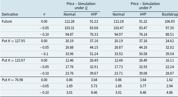
In Table 5, the differences of prices obtained under the normal and HYP assumptions are very small for the future contract and put options with $K=236.11$ and $K=229.62$ . The differences in prices obtained using the bootstrap approach and the HYP distribution are larger for these derivatives. This finding is consistent with the observation that the mean values of simulated $\text{CWSI}_{[t_0,t_1]}^{(1)}$ are very close under the two parametric distributions but higher using bootstrap from Fig. 5.

For the put options with $K=201.40$ , the HYP assumption and the bootstrap yield similar prices, with both being lower than the prices obtained under the normal assumption. In Fig. 5, we observe that the densities of simulated $\text{CWSI}_{[t_0,t_1]}^{(1)}$ for $\text{CWSI}_{[t_0,t_1]}^{(1)}\lt 201.40$ are generally higher under the normal assumption than they are under the HYP assumption. Therefore, the probability of non-zero option payoffs is also higher under the normal assumption, resulting in a higher option price. On the other hand, the left tails of the density curves under the HYP assumption and the bootstrap approach are close to each other, thereby explaining the close prices under the two assumptions. Therefore, the left tails of the density curves in Fig. 5 play a key role in the price of this option.

Table 5 indicates that the pricing error arising from misspecified distribution (normal) is small for futures and put options with relatively high strikes written on $\text{CWSI}_{[t_0,t_1]}^{(1)}$ . The semi-parametric model can only reduce the pricing error for options with low strikes.

In Table 6, the normal and HYP assumptions lead to very large price differences for all the derivatives written on $\text{CWSI}_{[t_0,t_1]}^{(2)}$ . Fig. 5 shows that the mean values of simulated $\text{CWSI}_{[t_0,t_1]}^{(2)}$ under the normal assumption are much higher than those under the HYP distribution. As a result, the normal assumption leads to higher prices for futures and lower prices for put options. The differences in prices obtained under the HYP assumption and the bootstrap approach are smaller than those obtained under the normal and HYP distributions. Therefore, the pricing error arising from misspecified distribution is very high for derivatives written on $\text{CWSI}_{[t_0,t_1]}^{(2)}$ . The semi-parametric model can partially reduce the pricing error.