Unit of analysis

The unit of analysis for this study is locality-year. The localities are metropolitan statistical areas (MSAs), which are socio-economic entities, not political jurisdictions. They are defined by the Office of Management and Budget as major urban centers plus the surrounding counties from which they draw their labor force.

MSAs are the appropriate unit because their average pollution levels reflect what the average person experiences on a daily basis at home and at work. Furthermore, because most air pollution at a given location is from nearby socio-economic activities, the policy efforts most relevant for influencing a person’s pollution exposure are those carried out within the same MSA.

Public opinion

I measure public opinion with the Google Trends internet search index, which indicates the annual proportion of air pollution-related searches in each locality. For the primary models presented below, the search index values are for the following combination of terms: smog + no2 + air pollution + ozone + pm2.5 + AQI. In Appendix B in the Supplementary material, I show results that exclude the term AQI to demonstrate robustness.

Fundamentally, search indexes like Google Trends reflect an issue’s salience – when people perceive an issue to be an urgent problem, they spend more time looking it up online (Reilly et al. Reference Reilly, Richey and Taylor2012; Mellon Reference Mellon2013). Salience is distinct from preferences, which refer to how much the public wants the government to do about an issue. Salience and preferences are not necessarily correlated; there can simultaneously be both broad agreement that an issue is an urgent problem and sharply divergent views about how much the government should do about it.

The air pollution issue domain is a special case in which salience and preferences closely correspond. In their 2017 study, Oehl, Schaffer, and Bernauer compare Google Trends data to survey measures of policy preferences. They establish that the public’s attention to an issue and the degree to which it wants the government to do more about it are highly correlated in domains related to air pollution emissions. Thus, in the context of this study, the search index reflects both salience and preferences. Hereafter, I use the term public concern to refer to this special case of public opinion.

The public concern variable is based on Google Trends data for designated market areas (DMAs). ^{Footnote 8} DMAs are the smallest geographic unit for which Google Trends data are available nationwide. There are 210 DMAs, which cover the entire US. Most are centered on metropolitan hubs, meaning their boundaries tend to roughly correspond with those of large- and mid-sized MSAs. Ohio’s Cleveland–Akron–Canton area, for instance, is both an MSA and a DMA. Many smaller MSAs straddle the boundaries between two or more DMAs. For these MSAs, public concern is calculated as the mean Google Trends value for the DMAs the MSA overlaps. Measurement error is almost certainly higher for the smaller MSAs that straddle multiple DMAs, which increases the noisiness of statistical estimates and biases them away from significance. Fortunately, the size of this measurement error appears to be modest; dropping smaller MSAs from the sample yields statistical estimates that are comparable to those shown in the analysis section.

Because DMAs cover the entire US, they include rural areas that are not part of any MSA. The Google Trends values for most MSAs therefore include internet traffic in adjacent rural areas. Due to their relatively small populations and low rates of internet connectivity, searches in rural areas are unlikely to meaningfully affect the Google Trends measure. This is especially true for searches related to air pollution, which tends to be more salient in urban areas. To the extent internet traffic in adjacent rural areas introduces measurement error, it should bias the analysis against finding significant relationships.

Policy

Policy is measured by aggregating all enforcement actions of the Clean Air Act (CAA) that take place in states and localities each year. The enforcement actions consist of ongoing federally reportable violations (FRVs), ongoing high-priority violations (HPVs), formal disciplinary actions (e.g. issuing fines), and informal disciplinary actions (e.g. issuing notices of noncompliance). These actions are undertaken by authorities at all levels of the political system. ^{Footnote 9}

I aggregate all actions that take place within the states and localities, regardless of which levels of the political system execute them. This is appropriate because the policy efforts relevant to air pollution levels in an area are not specific to any one level of government.

Outcomes

I measure ground-level air pollution outcomes with two ubiquitous pollutants – nitrogen dioxide ( ${\rm{N}}{{\rm{O}}_2}$ ) and fine particulate matter ( ${\rm{P}}{{\rm{M}}_{2.5}}$ ) – which are indicative of a locality’s overall air pollution level. ${\rm{N}}{{\rm{O}}_2}$ and ${\rm{P}}{{\rm{M}}_{2.5}}$ typically have correlations of over 0.7 with other major air pollutants, including course particulate matter (PM $_{10}$ ), carbon monoxide (CO), and sulfur dioxide (SO $_2$ ) (Guo et al. Reference Guo, Wang and Zhang2017). ^{Footnote 10}

${\rm{N}}{{\rm{O}}_2}$ is the primary pollution measure for this analysis because it closely reflects local emissions, while ${\rm{P}}{{\rm{M}}_{2.5}}$ is more sensitive to emissions region-wide. ${\rm{N}}{{\rm{O}}_2}$ has a short lifespan, which is comparable to other non-particulate air pollutants. It persists in the lower atmosphere for around one to two days before breaking down, so most ${\rm{N}}{{\rm{O}}_2}$ does not travel beyond the local area of its emission source. ${\rm{P}}{{\rm{M}}_{2.5}}$ , on the other hand, is an exceptionally long-lived air pollutant. It persists for days or weeks and can travel many hundreds of kilometers before falling out of the lower atmosphere (Jeong et al. Reference Jeong, Kim, Lee and Lee2017).

I leverage the different lifespans of these two pollutants in the empirical analysis. Comparing them makes it possible to infer the degree to which pollution changes are driven by local factors as opposed to regional or national influences.

${\rm{N}}{{\rm{O}}_2}$ and ${\rm{P}}{{\rm{M}}_{2.5}}$ concentrations are calculated with daily satellite overpass data. The ${\rm{N}}{{\rm{O}}_2}$ data are from the DOMINO (version 2) and TM4NO2A (version 2.3) datasets provided by the European Space Agency (ESA). The ${\rm{P}}{{\rm{M}}_{2.5}}$ data are from the Global Annual PM $_{2.5}$ Grids provided by NASA’s Socioeconomic Data and Applications Center. I discuss the details of how I process the data in Appendix F in the Supplementary material.

Measurement validity

While these measures are somewhat unconventional in political science, they are nevertheless exceptionally well suited for this study because they are direct, independent measures of the concepts of interest. The Google Trends measure reflects actual human behavior associated with concern (Swearingen and Ripberger Reference Swearingen and Ripberger2014). This sidesteps a major limitation of survey responses, which do not necessarily reflect people’s actual perceptions (see Bullock et al. Reference Bullock, Gerber, Hill and Huber2015). Google Trends also has higher spatial and temporal resolution than is feasible with surveys.

The CAA enforcement measure is a better measure of policy variation than more conventional measures, as implementation efforts vary considerably even without statutory changes (Wood and Waterman Reference Wood and Waterman1993). ^{Footnote 11}

${\rm{N}}{{\rm{O}}_2}$ and ${\rm{P}}{{\rm{M}}_{2.5}}$ concentrations are objective measurements of policy outcomes. They are validated by ESA and NASA and are entirely independent of the other concepts of interest. They do not depend on ground sensors, the distribution of which is influenced by pollution severity, policy efforts, and public opinion.

Partisanship

Partisanship can affect citizens’ environmental concerns and how they process information. Those affiliated with the Democratic Party are more inclined to becoming concerned with environmental issues when they observe deteriorating conditions (Egan and Mullin Reference Egan and Mullin2012). I therefore control for local partisanship in models with public concern as the DV. I measure partisanship as each locality’s average Democratic presidential candidate vote share for the time period of this study.

Economic output

Economic output must be controlled for in models with air pollution as the DV. This is because nearby economic activity is the primary driver of local air pollution in general and non-particulate pollutants like ${\rm{N}}{{\rm{O}}_2}$ in particular (Chan and Yao Reference Chan and Yao2008; Jiang et al. Reference Jiang, Lin and Lin2014; Jeong et al. Reference Jeong, Kim, Lee and Lee2017). Local economic output (i.e. gross regional product – GRP) values are from the Bureau of Economic Analysis and inflation adjusted.

Pollution spillover

Spillover is not a serious concern for ${\rm{N}}{{\rm{O}}_2}$ because it breaks down quickly in the atmosphere. The models presented below therefore simply ignore it. As a robustness check, I account for statewide ${\rm{N}}{{\rm{O}}_2}$ levels and find consistent results (see Appendix D in the Supplementary material). ^{Footnote 12} Nonlocal emissions are a major contributor to local ${\rm{P}}{{\rm{M}}_{2.5}}$ . This makes ${\rm{P}}{{\rm{M}}_{2.5}}$ levels less sensitive to local events, but there is no reason that spillover would bias measurement of ${\rm{P}}{{\rm{M}}_{2.5}}$ itself or its estimated relationships with other variables of interest.

Unmeasured determinants of public concern and air pollution

There are, of course, variables beyond those listed above that influence public concern and air pollution. Most notably, demographic characteristics like race and education are associated with environmental attitudes (Egan and Mullin Reference Egan and Mullin2012), and geography and climate are major determinants of air pollution levels (Chan and Yao Reference Chan and Yao2008; Jiang et al. Reference Jiang, Lin and Lin2014; Jeong et al. Reference Jeong, Kim, Lee and Lee2017).

I use lagged dependent variables (LDVs) to control for unmeasured factors like these. An LDV reflects all determinants of the DV’s value in the previous year, so it controls for any unmeasured EVs that do not change substantially from 1 year to the next. As an additional precaution, I use state fixed effects to control for any unmeasured regional factors that are not accounted for by the locality-specific LDVs.

Unmeasured policy

CAA enforcement actions are a good measure of policy efforts that explicitly target air pollution. However, many of the policy tools state and local authorities use to address air pollution do not explicitly target emissions. Examples of these tools include zoning rules, building permits, and other regulations and incentives that influence the locations of pollution sources.

Information about non-explicit policy is unlikely to be a significant factor driving public concern. Due to its obscure nature, the public almost certainly uses far less information about non-explicit policy than about explicit policy and visible outcomes.

Although the efforts themselves are difficult to observe, the aggregate impact of non-explicit policy on air pollution is significant (Monogan et al. Reference Monogan, Konisky and Woods2016). Studies that infer non-explicit policy variation through air pollution outcomes suggest that non-explicit policy efforts are highly responsive to local public opinion (Pargal et al. Reference Pargal, Hettige, Singh and Wheeler1997; Pinault et al. Reference Pinault, Crouse, Jerrett, Brauer and Tjepkema2016; Huang et al. Reference Huang, Santibanez-Gonzalez and Song2018).

Naive models

The system of relationships can be expressed as a trio of independent linear models and estimated with ordinary least squares (OLS). In Equations 1, 2, and 3, Search is the Google Trends search index that measures public concern. Enforce is CAA enforcement actions, which measure policy. NO2 is the concentration of the nitrogen dioxide air pollutant, which measures outcomes. Models that measure outcomes with ${\rm{P}}{{\rm{M}}_{2.5}}$ replace each instance of ${\rm{N}}{{\rm{O}}_2}$ with ${\rm{P}}{{\rm{M}}_{2.5}}$ and are otherwise identical (see Appendix E in the Supplementary material). GRP is gross regional product, which refers to local economic output. The $\Delta $ ’s signify year-on-year change. The $\alpha $ ’s are intercepts, the $\beta $ ’s are coefficient estimates, the e’s are error terms, and the $\hat \gamma $ ’s are vectors of control variables. The i and t subscripts refer to the locality and year of each observation, respectively. Note that each coefficient, vector, intercept, and error term has one or two subscript numbers. These indicate that the values are unique (e.g. the first $\beta $ in Equation 1 is different from the other $\beta $ ’s in the same equation and the first $\beta $ ’s in Equations 2 and 3):

(1) $${\eqalign{ Searc{h_{i,t}} = {\alpha _{1,0}} + {\beta _{1,1}}Searc{h_{i,t - 1}} + {\beta _{1,2}}\Delta NO{2_{i,t}} + {\beta _{1,3}}\Delta Enforc{e_{i,t}} \cr + {\beta _{1,4}}\Delta Statewide\;NO{2_{i,t}} + {\beta _{1,5}}\Delta Statewide\;Enforc{e_{i,t}} + {{\hat \gamma }_{1,i}} + {e_{1,i,t}} \cr}} $$

(2) $${\eqalign{ Enforc{e_{i,t}} = {\alpha _{2,0}} + {\beta _{2,1}}Enforc{e_{i,t - 1}} + {\beta _{2,2}}\Delta Searc{h_{i,t - 1}} + {\beta _{2,3}}\Delta NO{2_{i,t - 1}} \cr + {\beta _{2,4}}\Delta Statewide\;Searc{h_{i,t - 1}} + {\beta _{2,5}}\Delta Statewide\;NO{2_{i,t - 1}} + {{\hat \gamma }_{2,i}} + {e_{2,i,t}} \cr}} $$

(3) $${\eqalign{ NO{2_{i,t}} = {\alpha _{3,0}} + {\beta _{3,1}}NO{2_{i,t - 1}} + {\beta _{3,2}}\Delta GR{P_{i,t}} + {\beta _{3,3}}\Delta Searc{h_{i,t - 1}} + {\beta _{3,4}}\Delta Enforc{e_{i,t - 1}} \cr + {\beta _{3,5}}\Delta Statewide\;Searc{h_{i,t - 1}} + {\beta _{3,6}}\Delta Statewide\;Enforc{e_{i,t - 1}} + {{\hat \gamma }_{3,i}} + {e_{3,i,t}} \cr}} $$

Structural equation models

The equations above are estimated as three independent models. If the theory underlying these equations is correct, however, the relationships they depict form a dynamic system in which some combination of policy and outcomes affects public concern, which then goes on to affect policy and outcomes. The naive estimates shown in Figure 1 (and Table 1) in the next section suggest a robust dynamic between the search index and ${\rm{N}}{{\rm{O}}_2}$ – the search index has a strong effect on ${\rm{N}}{{\rm{O}}_2}$ , and ${\rm{N}}{{\rm{O}}_2}$ has a strong effect on the search index. If this pair of relationships does indeed reflect a process feeding back on itself, the search index and ${\rm{N}}{{\rm{O}}_2}$ should have correlated errors and biased estimates. The magnitude of bias from feedback is typically quite modest and can generally be ignored during estimation (see Hermida Reference Hermida2015). Nevertheless, the presence (or absence) of this bias provides additional evidence for (or against) the existence of a dynamic process.

Figure 1. Results summary

Note: The arrows represent causal relationships. The dashed arrows indicate effects that are predicted to be weak relative to the other effects on the search index. The coefficients correspond to those of Model 3 in Tables 1 and C.1 in the Supplementary material. $^\dagger p \lt $ 0.1; $^*p \lt $ 0.05; $^{**}p \lt $ 0.01; $^{***}p \lt $ 0.001.

Table 1. Regressions with NO₂

Note: All models include state fixed effects. The models in subtable a control for each locality’s Democratic vote share in presidential elections. $^\dagger p \lt 0.1$ ; $^*p \lt $ 0.05; $^{**}p \lt $ 0.01; $^{***}p \lt $ 0.001.

If the theorized dynamic exists, the naive estimates for ${\rm{N}}{{\rm{O}}_2}$ ’s effect on the search index and the search index’s effect on ${\rm{N}}{{\rm{O}}_2}$ should be biased towards zero because the two relationships have opposite signs (i.e. the search index’s effect on ${\rm{N}}{{\rm{O}}_2}$ has the opposite sign of ${\rm{N}}{{\rm{O}}_2}$ ’s effect on the search index). ^{Footnote 13} This bias is introduced by unmeasured shocks to public concern and air pollution that persist over time. A shock that increases public concern – new high-profile medical research on pollution’s health consequences, for instance – would cause ${\rm{N}}{{\rm{O}}_2}$ to decrease the following year via responsive policy. If the shock dissipated quickly, it would be like any other source of random error; it would inflate the unexplained variation of the search index but would not introduce bias. If, however, the shock’s effect on concern persisted for multiple years, the search index would remain high even as contemporary ${\rm{N}}{{\rm{O}}_2}$ levels continued to decrease. This would bias pollution severity’s estimated effect on the search index in the negative direction (i.e. towards zero). Similarly, a shock to air pollution that persisted would bias the search index’s estimated effect on it in the positive direction. If an exogenous event like natural gas prices falling relative to coal caused a multi-year decrease in pollution levels, those lower levels would decrease public concern as measured by the search index. If, as the search index decreased, the shock continued to reduce pollution levels, the search index’s estimated effect on ${\rm{N}}{{\rm{O}}_2}$ would be biased in the positive direction (i.e. towards zero).

I use structural equation models (SEMs) to test for the error correlation and bias the theorized dynamic should create. An SEM can specify error correlation between specific variables, which is accounted for when the model is estimated. I compare the performance of an SEM that specifies error correlation between the search index and ${\rm{N}}{{\rm{O}}_2}$ to an otherwise identical SEM that does not. If the dynamic exists, then the effects of Search and NO2 on one another should be (modestly) larger – and the relative fit better – for the SEM that specifies the expected error correlation:

(4) $$\eqalign{ Searc{h_{i,t - 1}} = {\alpha _{4,0}} + {\beta _{4,1}}Searc{h_{i,t - 2}} + {\beta _{4,2}}\Delta NO{2_{i,t - 1}} + {\beta _{4,3}}NO{2_{i,t - 1}} \cr + {\beta _{4,4}}\Delta Enforc{e_{i,t - 1}} + {\beta _{4,5}}Enforc{e_{i,t - 1}} + {{\hat \gamma }_{4,i}} + {e_{4,i,t - 1}} \cr} $$

(5) $$\eqalign{ Enforc{e_{i,t}} = {\alpha _{5,0}} + {\beta _{5,1}}Enforc{e_{i,t - 1}} + {\beta _{5,2}}Searc{h_{i,t - 1}} \cr + {\beta _{5,3}}\Delta NO{2_{i,t - 1}} + {\beta _{5,4}}NO{2_{i,t - 1}} + {{\hat \gamma }_{5,i}} + {e_{5,i,t}} \cr} $$

(6) $$\eqalign{ NO{2_{i,t}} = {\alpha _{6,0}} + {\beta _{6,1}}NO{2_{i,t - 1}} + {\beta _{6,2}}\Delta GR{P_{i,t}} + {\beta _{6,3}}Searc{h_{i,t - 1}} \cr + {\beta _{6,4}}Enforc{e_{i,t - 1}} + {\beta _{6,5}}\Delta Enforc{e_{i,t - 1}} + {{\hat \gamma }_{6,i}} + {e_{6,i,t}} \cr} $$

Note that Search, Enforce, and NO2 are included as EVs in the SEM equations, and that the Search DV is lagged by 1 year (with its EVs lagged accordingly) so that it matches the lag of the Search EV in the NO2 equation. This is necessary for estimating error correlation between the search index and ${\rm{N}}{{\rm{O}}_2}$ .

Public opinion’s responsiveness to information

The four variables’ effects on the search index shown in Figure 1(a) and (b) reflect the degree to which the public uses information about each to update its concerns. Local ${\rm{N}}{{\rm{O}}_2}$ and statewide enforcement’s highly significant effects indicate that the public uses information about local air pollution outcomes and statewide policy. Local ${\rm{N}}{{\rm{O}}_2}$ ’s positive sign shows that the public becomes more concerned with air pollution as the problem becomes worse in daily life. Statewide enforcement’s negative sign shows that the public becomes less concerned with air pollution as governmental authorities do more to mitigate the problem statewide. The magnitudes of local ${\rm{N}}{{\rm{O}}_2}$ and statewide policy’s effects are substantively meaningful, with local ${\rm{N}}{{\rm{O}}_2}$ ’s effect being the larger of the two. A one standard deviation increase of local ${\rm{N}}{{\rm{O}}_2}$ would increase the search index by 0.13 standard deviations, a 9% change for the average observation. A one standard deviation increase of statewide enforcement would decrease the search index by 0.10 standard deviations, a 7% change for the average observation. ^{Footnote 15}

Local enforcement and statewide ${\rm{N}}{{\rm{O}}_2}$ ’s effects on the search index are statistically and substantively weak, which suggests the public uses relatively little information about local policy and statewide outcomes to update its concerns. Statistically, local enforcement’s effect straddles the conventional significance threshold; its p-value is slightly below the 0.05 threshold in the model as shown in Figure 1 (p = 0.04) and above it in the alternate model as shown in Table 1 (p = 0.37). Substantively, a one standard deviation increase in local enforcement would increase the search index by 0.03 standard deviations, a 2% change for the average observation. Statewide ${\rm{N}}{{\rm{O}}_2}$ ’s effect on the search index is practically nonexistent; its magnitude is negligible and is nowhere near statistical significance (p $ \gt $ 0.9).

The relative sizes of these four effects are consistent with my central argument. While all the policy and outcomes information measured in this study is available to anyone who wants it, public concern is consistently more responsive to the information that is more readily accessible. This suggests that the public’s responsiveness to information is conditioned by the information’s accessibility. There are no clear alternative explanations that can account for the dominant effects of both local outcomes and statewide policy on public concern. Together, these effects rule out the possibility that the public’s use of available information is driven by a strong preference for policy information over outcomes information (or vice versa), or local information over statewide information (or vice versa).

Policy outcomes’ responsiveness to public opinion

The search index’s effect on air pollution reflects the outcomes of policy prompted by public concern. It is possible to infer policy outcomes’ responsiveness to the public with this relationship because policy is the only mechanism through which public sentiment can significantly affect air pollution within the time span of this analysis. Popular concern can prompt individual-level behaviors that meaningfully affect air pollution without governmental action, but only on timescales dramatically shorter or longer than this analysis. For example, while severe smog often leads people to delay travel plans for days or weeks (Barwick et al. Reference Barwick, Li, Liguo and Zou2019), such behavioral changes have no net impact on pollution emissions over the course of an entire year (Welch et al. Reference Welch, Gu and Kramer2005). Without policy intervention, public concern only leads to durable changes in individual-level pollution-generating activities (e.g. driving habits) on timescales of a decade or longer (see Tribby et al. Reference Tribby, Miller, Song and Smith2013). ^{Footnote 16}

It is necessary to infer responsiveness from the search index’s “direct” effect on air pollution because the enforcement variable is only a partial measure of total policy effort in a given geographic area. As discussed above, CAA enforcement actions do not reflect non-explicit policy efforts like the strategic use of zoning rules and building permits to influence the placement of emission sources. There is ample evidence that state and local officials regularly use non-explicit policy tools to address air pollution problems in their jurisdictions, and that their use of these policy tools is sensitive to public opinion (Pargal et al. Reference Pargal, Hettige, Singh and Wheeler1997; Monogan et al. Reference Monogan, Konisky and Woods2016; Pinault et al. Reference Pinault, Crouse, Jerrett, Brauer and Tjepkema2016; Huang et al. Reference Huang, Santibanez-Gonzalez and Song2018).

The search index’s estimated effect on air pollution strongly suggests that unmeasured policy is responsive to local public concern. If unmeasured policy efforts are prompted by local shifts in public concern, a robust negative effect of the search index on local air pollution is what we should see. Local-level policy responsiveness is further evidenced by the relative sizes of the search index’s effects on ${\rm{N}}{{\rm{O}}_2}$ and ${\rm{P}}{{\rm{M}}_{2.5}}$ , as searches’ negative effect on ${\rm{N}}{{\rm{O}}_2}$ is significantly stronger than it is on ${\rm{P}}{{\rm{M}}_{2.5}}$ (see Appendix E in the Supplementary material). Given that a higher proportion of the former is from local sources, the search index’s larger effect on ${\rm{N}}{{\rm{O}}_2}$ implies the phenomenon that accounts for these effects is, to a significant degree, local.

The relative sizes of the effects on ${\rm{N}}{{\rm{O}}_2}$ and ${\rm{P}}{{\rm{M}}_{2.5}}$ are also evidence against a major unmeasured exogenous event causing a spurious relationship between searches and air pollution. If, for instance, the relationship were due to a dramatic environmental catastrophe that shocked government officials into action and drew public attention nationwide, the search index’s estimated effect on ${\rm{N}}{{\rm{O}}_2}$ would likely be smaller (or, at the very least, not significantly bigger) than its effect on ${\rm{P}}{{\rm{M}}_{2.5}}$ .

The weakness of the search index’s effect on the enforcement variable indicates that measured policy is not immediately responsive to local public concern. If it were, the search index’s effect would be significantly positive. CAA enforcement actions are carried out by specialized regulatory entities, which tend to be less sensitive to public concern – and more sensitive to objective problem severity – than other governmental bodies (Mullin Reference Mullin2008). Thus, it is unsurprising that measured policy is not immediately responsive to public concern. That said, this analysis only assesses policy’s responsiveness to year-on-year changes in public concern; it does not rule out the possibility that CAA enforcement actions are responsive to public concern changes on larger timescales.

Further evidence of a dynamic process

In Table 2, the second model is an SEM that specifies error correlation between the search index and ${\rm{N}}{{\rm{O}}_2}$ . The first model is an SEM that assumes the two variables are independent but is otherwise identical to Model 2. As discussed previously, any error correlation from the theorized dynamic should bias the relationships of interest towards zero. Thus – if the dynamic exists – ignoring it should lead to smaller estimates for $\Delta {\rm{N}}{{\rm{O}}_2}$ ’s effect on the search index and the search index’s effect on ${\rm{N}}{{\rm{O}}_2}$ . This is exactly what we see. Moreover, Model 2’s smaller AIC and SABIC values indicate that it has better overall fit than Model 1. ^{Footnote 20}

Table 2. SEM results

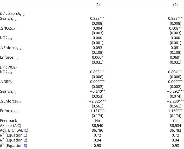
Note: N = 4,679. Estimator: ML. The search equation has year fixed effects. The NO2 equation has state fixed effects. Estimated using “lavaan” v0.6–2 in R Open 3.5.1. $^\dagger p \lt 0.1$ ; $^{*}p \lt $ 0.05; $^{**}p \lt $ 0.01; $^{***}p \lt $ 0.001.