


1. Introduction
During the first half of the 20th century, astronomers developed several empirical functions to describe the observed, that is, projected on the plane of the sky, radial distribution of light in external galaxies. These functions provided physical measurements which enabled astronomers to better answer simple questions such as, How big is it, and, How bright is it? This helped to place extragalactic astronomy on a more scientific footing, elevating some sky surveys above the somewhat derogatory status of ‘stamp collecting’.
For both early-type galaxies (ETGs) and late-type galaxies (LTGs), these mathematical functions had two parameters: one stretched the model light profile along the horizontal (radial) axis and the other stretched it along the vertical (intensity) axis. One could arbitrarily set the scale radius to be where the intensity had dropped by some fixed factor from the central intensity, or it could be set as the radius effectively enclosing some fixed fraction of the total light, such as 50% or 90%. Due to the homologous nature of these two-parameter models, defining the scale radius or the scale intensity in a different way would shift all galaxies equally in diagrams involving the logarithm of these model-determined quantities. As such, trends and patterns in such diagrams were not dependent on how these scale parameters were set. However, if galaxies are not adequately described by these two-parameter functions, then the galaxies’ distribution in the scaling diagrams can become a function of the arbitrarily defined scale radius and scale intensity.
The above fact, and the implications of the above fact, has not been adequately realised in the literature, and countless papers have drawn questionable scientific conclusions based upon the distribution of galaxies in diagrams involving a galaxies’ arbitrary 50% radius and the intensity associated with this radius. Given that this has gone on for decades, this paper goes to some length to try and carefully explain the curved distribution of ETGs in diagrams involving effective half-light parameters. These curved distributions have been used many times in the literature to argue for a distinct divide among the ETG population into dwarf and giantFootnote a ETGs separated at the bend midpoint:
 $\mathfrak{M}_B
\approx -18$
mag (e.g. Kormendy et al., Reference Kormendy, Fisher, Cornell and Bender2009, hereafter K09; Kormendy & Bender, Reference Kormendy and Bender2012; Kormendy, Reference Kormendy, Laurikainen, Peletier and Gadotti2016; Tolstoy, Hill, & Tosi, Reference Tolstoy, Hill and Tosi2009; Somerville & Davé, Reference Somerville and Davé2015). In order to help better appreciate this issue and more fully understand galaxy structure, the curved distributions of ETGs in diagrams involving radii that enclose different percentages of the total light are presented, and it is revealed how the absolute magnitude associated with the midpoint of the bend changes considerably.
$\mathfrak{M}_B
\approx -18$
mag (e.g. Kormendy et al., Reference Kormendy, Fisher, Cornell and Bender2009, hereafter K09; Kormendy & Bender, Reference Kormendy and Bender2012; Kormendy, Reference Kormendy, Laurikainen, Peletier and Gadotti2016; Tolstoy, Hill, & Tosi, Reference Tolstoy, Hill and Tosi2009; Somerville & Davé, Reference Somerville and Davé2015). In order to help better appreciate this issue and more fully understand galaxy structure, the curved distributions of ETGs in diagrams involving radii that enclose different percentages of the total light are presented, and it is revealed how the absolute magnitude associated with the midpoint of the bend changes considerably.
Advocates for an ETG dichotomy have alleged that the formation physics must be dramatically different for ETGs fainter and brighter than
 $\mathfrak{M}_B
\approx -18$
mag, because the slope of certain scaling relations is different at magnitudes fainter and brighter than this. For example, Kormendy & Djorgovski (Reference Kormendy and Djorgovski1989; see their Section 8) wrote, ‘A fundamental application of parameter correlations has been the demonstration that diffuse dwarf spheroidalFootnote b galaxies are a family of objects unrelated to ellipticals’. This claim was, however, at odds with other research that did not use effective half-light parameters and instead advocated for a continuity among the ETG population at
$\mathfrak{M}_B
\approx -18$
mag, because the slope of certain scaling relations is different at magnitudes fainter and brighter than this. For example, Kormendy & Djorgovski (Reference Kormendy and Djorgovski1989; see their Section 8) wrote, ‘A fundamental application of parameter correlations has been the demonstration that diffuse dwarf spheroidalFootnote b galaxies are a family of objects unrelated to ellipticals’. This claim was, however, at odds with other research that did not use effective half-light parameters and instead advocated for a continuity among the ETG population at $\mathfrak{M}_B \approx -18$
mag (e.g. Caldwell, 1983a, see his Figure 6; Binggeli, Sandage, Tarenghi, Reference Binggeli, Sandage and Tarenghi1984; Sandage et al. Reference Sandage, Binggeli and Tammann1985; Binggeli, Sandage, & Tammann Reference Binggeli, Sandage and Tammann1985; Bothun et al., Reference Bothun, Mould, Caldwell and MacGillivray1986, see their Figure 7; Caldwell & Bothun, Reference Caldwell and Bothun1987).
$\mathfrak{M}_B \approx -18$
mag (e.g. Caldwell, 1983a, see his Figure 6; Binggeli, Sandage, Tarenghi, Reference Binggeli, Sandage and Tarenghi1984; Sandage et al. Reference Sandage, Binggeli and Tammann1985; Binggeli, Sandage, & Tammann Reference Binggeli, Sandage and Tammann1985; Bothun et al., Reference Bothun, Mould, Caldwell and MacGillivray1986, see their Figure 7; Caldwell & Bothun, Reference Caldwell and Bothun1987).
As noted by James (Reference James1994), the shape of ETG light profiles had also been considered one of the principal differences separating dwarf and ordinary ETGs — with ‘dwarf’ ETGs having exponential light profiles (similar to the discs of LTGs) and ‘ordinary’ ETGs having $R^{1/4}$
profiles — emboldening those interpreting transitions in certain scaling diagrams as evidence of different formation physics at magnitudes fainter and brighter than
$R^{1/4}$
profiles — emboldening those interpreting transitions in certain scaling diagrams as evidence of different formation physics at magnitudes fainter and brighter than $\mathfrak{M}_B \approx -18$
mag. However, as we shall see, the systematically changing (with absolute magnitude) shape of the ETG light profile, that is, structural non-homology, is key to understanding the unification of dwarf and ordinary ETGs.
$\mathfrak{M}_B \approx -18$
mag. However, as we shall see, the systematically changing (with absolute magnitude) shape of the ETG light profile, that is, structural non-homology, is key to understanding the unification of dwarf and ordinary ETGs.
To understand the mechanics of the structural parameter scaling diagrams, Section 2 of this paper provides a context-setting background using de Vaucouleurs’ $R^{1/4}$
model and Sérsic’s
$R^{1/4}$
model and Sérsic’s $R^{1/n}$
model, and provides a familiarity with the model parameters
$R^{1/n}$
model, and provides a familiarity with the model parameters $R_{\rm e}$
and both the surface brightness at
$R_{\rm e}$
and both the surface brightness at $R_{\rm e}$
, denoted by
$R_{\rm e}$
, denoted by $\mu_{\rm e}$
, and the average surface brightness within
$\mu_{\rm e}$
, and the average surface brightness within $R_{\rm e}$
, denoted by
$R_{\rm e}$
, denoted by $\langle\mu\rangle_{\rm e}$
. Section 3 then presents two key empirical relations, providing the foundation for the insight which follows.
$\langle\mu\rangle_{\rm e}$
. Section 3 then presents two key empirical relations, providing the foundation for the insight which follows.
Equipped with the above background knowledge, Section 4 presents an array of scaling relations based on radii and surface brightnesses which effectively enclose different fixed percentages of the galaxy light. It soon becomes apparent why the $\mu_{\rm e}$
–
$\mu_{\rm e}$
– $R_{\rm e}$
relation is itself quite tight for bright ETGs but not for faint ETGs. 4.2 then goes on to explore a range of alternative radii and surface brightnesses. In particular, radii where the intensity has dropped by a fixed percentage are introduced, and the use of isophotal radii is revisited in 4.3. Section 5 expands on the analysis using internal radii that define spheres that effectively enclose a fixed percentage of the galaxy light. These internal radii include ‘effective’ radii plus the new radii where the internal density has declined by a fixed amount, isodensity radii, virial radii, and new Petrosian-like radii. The changing location of the bend midpoint in various scaling relations reveals that it has nothing to do with changing physical processes but is instead merely a result of the arbitrary definition used to quantify the sizes of ETGs.
$R_{\rm e}$
relation is itself quite tight for bright ETGs but not for faint ETGs. 4.2 then goes on to explore a range of alternative radii and surface brightnesses. In particular, radii where the intensity has dropped by a fixed percentage are introduced, and the use of isophotal radii is revisited in 4.3. Section 5 expands on the analysis using internal radii that define spheres that effectively enclose a fixed percentage of the galaxy light. These internal radii include ‘effective’ radii plus the new radii where the internal density has declined by a fixed amount, isodensity radii, virial radii, and new Petrosian-like radii. The changing location of the bend midpoint in various scaling relations reveals that it has nothing to do with changing physical processes but is instead merely a result of the arbitrary definition used to quantify the sizes of ETGs.
Section 6 presents ETG data from Ferrarese et al. (Reference Ferrarese, Côté and Jordán2006) and K09, and resolves the different interpretations given in those papers. Finally, a discussion in Section 7 broaches some of the literature which has advocated for a dichotomy of the ETG population at $\mathfrak{M}_B \approx -18$
mag. Considerable historical context is included to aid the reader in understanding how the topic evolved. This is also partly necessary because support for interpreting these curved relations, in terms of different formation processes at magnitudes brighter and fainter than the bend midpoint at
$\mathfrak{M}_B \approx -18$
mag. Considerable historical context is included to aid the reader in understanding how the topic evolved. This is also partly necessary because support for interpreting these curved relations, in terms of different formation processes at magnitudes brighter and fainter than the bend midpoint at $\mathfrak{M}_B \approx -18$
mag, attracted a range of bright ideas over the years and many of these are sometimes heralded without adequate qualification. Some of the literature surrounding the similar separation of bulges into ‘classical’ or ‘pseudobulge’ is also discussed. Bulge scaling relations, as distinct from ETG scaling relations, are also discussed in the context of high-z compact massive systems, which by all accounts appear to be the bulges of massive local galaxies. In addition, Subsection 7.5 reveals why the ‘Fundamental Plane’, involving the velocity dispersion
$\mathfrak{M}_B \approx -18$
mag, attracted a range of bright ideas over the years and many of these are sometimes heralded without adequate qualification. Some of the literature surrounding the similar separation of bulges into ‘classical’ or ‘pseudobulge’ is also discussed. Bulge scaling relations, as distinct from ETG scaling relations, are also discussed in the context of high-z compact massive systems, which by all accounts appear to be the bulges of massive local galaxies. In addition, Subsection 7.5 reveals why the ‘Fundamental Plane’, involving the velocity dispersion $\sigma$
(Djorgovski and Davis, Reference Djorgovski and Davis1987; see also Fish, Reference Fish1963), is tighter than the
$\sigma$
(Djorgovski and Davis, Reference Djorgovski and Davis1987; see also Fish, Reference Fish1963), is tighter than the $\mu_{\rm e}$
–
$\mu_{\rm e}$
– $R_{\rm e}$
relation for ordinary ETGs, and a warning about fitting and interpreting 2D planes to curved distributions involving supermassive black hole mass and ‘effective’ parameters is also issued.
$R_{\rm e}$
relation for ordinary ETGs, and a warning about fitting and interpreting 2D planes to curved distributions involving supermassive black hole mass and ‘effective’ parameters is also issued.
2. Mathematical background
2.1. de Vaucouleurs’ $R^{1/4}$
model
$R^{1/4}$
model

First in French (de Vaucouleurs, Reference de Vaucouleurs1948) then in English, de Vaucouleurs (Reference de Vaucouleurs1953) presented an empirical function that was to become known as the $R^{1/4}$
model due to how the projected (on the plane of the sky) intensity profile I(R) depends on the projected radius R raised to the 1/4 power. This mathematical model can be expressed as
$R^{1/4}$
model due to how the projected (on the plane of the sky) intensity profile I(R) depends on the projected radius R raised to the 1/4 power. This mathematical model can be expressed as
 \begin{equation}
I(R)=I_0\exp\left[ -b\left(\frac{R}{R_{\rm s}}\right) ^{1/4}\right] = \frac{I_0}{\left( {\rm e}^{b}\right)^{\left(R/R_{\rm s} \right)^{1/4}}},
\end{equation}
\begin{equation}
I(R)=I_0\exp\left[ -b\left(\frac{R}{R_{\rm s}}\right) ^{1/4}\right] = \frac{I_0}{\left( {\rm e}^{b}\right)^{\left(R/R_{\rm s} \right)^{1/4}}},
\end{equation}
where $R_{\rm s}$
is a scale radius,
$R_{\rm s}$
is a scale radius, $I_0$
is a scale intensity at
$I_0$
is a scale intensity at $R=0$
, and b is a constant that shall be explained below. Given that the galaxies do not have clear edges — and in the middle of the 20th century it was not known how their radial profiles behaved at large radii — the practice was to extrapolate one’s adopted model to infinity in order to determine a galaxy’s total luminosity.
$R=0$
, and b is a constant that shall be explained below. Given that the galaxies do not have clear edges — and in the middle of the 20th century it was not known how their radial profiles behaved at large radii — the practice was to extrapolate one’s adopted model to infinity in order to determine a galaxy’s total luminosity.
The projected luminosity (from three dimensions to two dimensions onto the plane of the sky) interior to a circle of radius R is determined by integrating the intensity over the enclosed area, such that
 \begin{equation}
L({\lt}R) = \int_0^R I(R^{\prime})2\pi R^{\prime} {\rm d}R^{\prime}.
\end{equation}
\begin{equation}
L({\lt}R) = \int_0^R I(R^{\prime})2\pi R^{\prime} {\rm d}R^{\prime}.
\end{equation}
Using the substitution $x=b(R/R_{\rm s})^{1/4}$
in equation (1), the above integral reduces to
$x=b(R/R_{\rm s})^{1/4}$
in equation (1), the above integral reduces to
 \begin{equation}
L({\lt}R)=\frac{I_0 R_{\rm s}^{2}8\pi}{b^8}\gamma (8,x),
\end{equation}
\begin{equation}
L({\lt}R)=\frac{I_0 R_{\rm s}^{2}8\pi}{b^8}\gamma (8,x),
\end{equation}
where $\gamma $
(8,x) is the incomplete gamma function defined by
$\gamma $
(8,x) is the incomplete gamma function defined by
 \begin{equation}
\gamma (8,x)=\int ^{x}_{0} {\rm e}^{-t}t^{8-1}{\rm d}t.
\label{eqn4}
\end{equation}
\begin{equation}
\gamma (8,x)=\int ^{x}_{0} {\rm e}^{-t}t^{8-1}{\rm d}t.
\label{eqn4}
\end{equation}
As noted, the total luminosity is obtained by integrating to infinity, in which case $\gamma (8,x)$
is replaced with the complete gamma function,
$\gamma (8,x)$
is replaced with the complete gamma function, $\Gamma (8)$
, and one has that
$\Gamma (8)$
, and one has that
 \begin{equation}
L_{\rm tot} = \frac{I_0 R_{\rm s}^{2}8\pi}{b^8}\Gamma (8).
\label{eqn5}
\end{equation}
\begin{equation}
L_{\rm tot} = \frac{I_0 R_{\rm s}^{2}8\pi}{b^8}\Gamma (8).
\label{eqn5}
\end{equation}
Now, here is where things can, and did, become arbitrary. Gerard de Vaucouleurs elected to define the radius $R_{\rm s}$
such that it enclosed 50% of the total light
$R_{\rm s}$
such that it enclosed 50% of the total light $L_{\rm tot}$
. He did this by determining the value of b required to balance the equation
$L_{\rm tot}$
. He did this by determining the value of b required to balance the equation
 \begin{equation}
\gamma (8,b) = 0.5\,\Gamma (8).
\label{eqn6}
\end{equation}
\begin{equation}
\gamma (8,b) = 0.5\,\Gamma (8).
\label{eqn6}
\end{equation}
With $b=-7.669$
, the projected radius
$b=-7.669$
, the projected radius $R_{\rm s}$
effectively encloses half of the model’s total light, and it was subsequently denoted
$R_{\rm s}$
effectively encloses half of the model’s total light, and it was subsequently denoted $R_{\rm e}$
and referred to as the ‘effective half light radius’. The
$R_{\rm e}$
and referred to as the ‘effective half light radius’. The $R^{1/4}$
model’s central surface brightness,
$R^{1/4}$
model’s central surface brightness, $\mu_0$
, is given by
$\mu_0$
, is given by $-2.5\log I_0$
, and the projected intensity at
$-2.5\log I_0$
, and the projected intensity at $R=R_s \equiv R_{\rm e}$
is given by
$R=R_s \equiv R_{\rm e}$
is given by
 \begin{equation}
I_{\rm e}=I_0{\rm e}^{-b} = I_0/2141.
\label{eqn7}
\end{equation}
\begin{equation}
I_{\rm e}=I_0{\rm e}^{-b} = I_0/2141.
\label{eqn7}
\end{equation}
The average intensity $\langle I \rangle_{\rm e}$
within
$\langle I \rangle_{\rm e}$
within $R_{\rm e}$
is such that
$R_{\rm e}$
is such that
 \begin{equation}
0.5\,L_{\rm tot} = \pi R_{\rm e}^2 \langle I \rangle_{\rm e},
\label{eqn8}
\end{equation}
\begin{equation}
0.5\,L_{\rm tot} = \pi R_{\rm e}^2 \langle I \rangle_{\rm e},
\label{eqn8}
\end{equation}
and it can be shown that
 \begin{equation}
\langle I \rangle_{\rm e} = 3.61 I_{\rm e} = I_0/594
\label{eqn9}
\end{equation}
\begin{equation}
\langle I \rangle_{\rm e} = 3.61 I_{\rm e} = I_0/594
\label{eqn9}
\end{equation}
(Graham & Driver, Reference Graham and Driver2005, see their equations 7 and 9).
As alluded to above, de Vaucouleurs could have chosen a radius enclosing any fraction of the light, and his two-parameter model would still have the same functional form (equation (1)). That is, one could use a radius $R_X$
containing any percentage of the total light, and one could use an intensity
$R_X$
containing any percentage of the total light, and one could use an intensity $I_Y$
taken from any (similar or different) fixed radius (in units of
$I_Y$
taken from any (similar or different) fixed radius (in units of $R_{\rm e}$
). The homology of the
$R_{\rm e}$
). The homology of the $R^{1/4}$
model is such that
$R^{1/4}$
model is such that $R_X = C_1 R_{\rm e}$
,
$R_X = C_1 R_{\rm e}$
, $I_Y = C_2 I_{\rm e}$
, and
$I_Y = C_2 I_{\rm e}$
, and $\langle I \rangle _Y = C_3 \langle I \rangle_{\rm e}$
, where
$\langle I \rangle _Y = C_3 \langle I \rangle_{\rm e}$
, where $C_1$
,
$C_1$
, $C_2,$
and
$C_2,$
and $C_3$
are constants. In trying to understand the behaviour of, and connections between, galaxies, astronomers could plot
$C_3$
are constants. In trying to understand the behaviour of, and connections between, galaxies, astronomers could plot $\log R_X$
versus
$\log R_X$
versus $-2.5\log I_Y$
, and versus
$-2.5\log I_Y$
, and versus $-2.5\log \langle I \rangle _Y$
, and the trends would be the same as obtained when using
$-2.5\log \langle I \rangle _Y$
, and the trends would be the same as obtained when using $R_{\rm e}$
,
$R_{\rm e}$
, $I_{\rm e,}$
and
$I_{\rm e,}$
and $\langle I \rangle_{\rm e}$
, just shifted vertically or horizontally in one’s diagram. As such, the arbitrary selection of 50% by de Vaucouleurs did not appear to matter. To give a more concrete example, de Vaucouleurs could have set the scale radius
$\langle I \rangle_{\rm e}$
, just shifted vertically or horizontally in one’s diagram. As such, the arbitrary selection of 50% by de Vaucouleurs did not appear to matter. To give a more concrete example, de Vaucouleurs could have set the scale radius
 $R_s
= R_{10}$
, that is, enclosing 10% of the total light (e.g. Farouki, Shapiro, & Duncan, Reference Farouki, Shapiro and Duncan1983). The mean intensity
$R_s
= R_{10}$
, that is, enclosing 10% of the total light (e.g. Farouki, Shapiro, & Duncan, Reference Farouki, Shapiro and Duncan1983). The mean intensity $\langle I \rangle_{10}$
within this radius is related by the expression
$\langle I \rangle_{10}$
within this radius is related by the expression
 \begin{equation}
0.1\,L_{\rm tot} = \pi R_{10}^2 \langle I \rangle_{10},
\label{eqn10}
\end{equation}
\begin{equation}
0.1\,L_{\rm tot} = \pi R_{10}^2 \langle I \rangle_{10},
\label{eqn10}
\end{equation}
and the associated value of b is obtained by solving the equation
 \begin{equation}
\gamma (8,b) = \Gamma (8)/10,
\label{eqn11}
\end{equation}
\begin{equation}
\gamma (8,b) = \Gamma (8)/10,
\label{eqn11}
\end{equation}
to give $b=4.656$
and
$b=4.656$
and $I_{10}=I_0{\rm e}^{-b} = I_0/105.2$
(cf. equation (7)). In this example, de Vaucouleurs’ model would then read
$I_{10}=I_0{\rm e}^{-b} = I_0/105.2$
(cf. equation (7)). In this example, de Vaucouleurs’ model would then read
 \begin{equation}
I(R)=I_0\exp\left[ \frac{-4.656}{R_{10}^{1/4}} R^{1/4}\right],
\label{eqn12}
\end{equation}
\begin{equation}
I(R)=I_0\exp\left[ \frac{-4.656}{R_{10}^{1/4}} R^{1/4}\right],
\label{eqn12}
\end{equation}
where $R_{10} = (4.656/7.669)^4\, R_{\rm e} = R_{\rm e}/7.361$
, and
$R_{10} = (4.656/7.669)^4\, R_{\rm e} = R_{\rm e}/7.361$
, and $\langle I \rangle_{10}=I_0/54.77$
.
$\langle I \rangle_{10}=I_0/54.77$
.
However, and this is the crux of the matter: ETGs, and also the bulges of spiral galaxies, do not follow the $R^{1/4}$
model, that is, there is not structural homology. This has important consequences when using radii enclosing a fixed percentage of the total light, and when using the associated surface brightness terms.
$R^{1/4}$
model, that is, there is not structural homology. This has important consequences when using radii enclosing a fixed percentage of the total light, and when using the associated surface brightness terms.
It is noted that the $R^{1/4}$
model had become so entrenched during the second half of the 20th century that it was invariably referred to as the
$R^{1/4}$
model had become so entrenched during the second half of the 20th century that it was invariably referred to as the $R^{1/4}$
law. That is, this empirical model was effectively elevated to the status of a physical law because it was thought that all ETGs did have
$R^{1/4}$
law. That is, this empirical model was effectively elevated to the status of a physical law because it was thought that all ETGs did have $R^{1/4}$
light profiles. Indeed, it was not uncommon for astronomers to vary the sky-background in order to make their light profiles more
$R^{1/4}$
light profiles. Indeed, it was not uncommon for astronomers to vary the sky-background in order to make their light profiles more $R^{1/4}$
-like (e.g. Tonry et al., Reference Tonry, Blakeslee, Ajhar and Dressler1997; see also the ‘Seven Samurai’ team data from Burstein et al., Reference Burstein, Davies and Dressler1987 as presented in D’Onofrio, Capaccioli, & Caon Reference D’Onofrio, Capaccioli and Caon1994, their Figure 4). This belief was in part because of de Vaucouleurs (Reference de Vaucouleurs and Flügge1959) study that had shown that the
$R^{1/4}$
-like (e.g. Tonry et al., Reference Tonry, Blakeslee, Ajhar and Dressler1997; see also the ‘Seven Samurai’ team data from Burstein et al., Reference Burstein, Davies and Dressler1987 as presented in D’Onofrio, Capaccioli, & Caon Reference D’Onofrio, Capaccioli and Caon1994, their Figure 4). This belief was in part because of de Vaucouleurs (Reference de Vaucouleurs and Flügge1959) study that had shown that the $R^{1/4}$
model fit better than the popular Reynolds’ (Reference Reynolds1913) modelFootnote c, and because of de Vaucouleurs & Capaccioli’s (Reference de Vaucouleurs and Capaccioli1979) study of NGC 3379 which revealed that its light profile is remarkably well fit by the
$R^{1/4}$
model fit better than the popular Reynolds’ (Reference Reynolds1913) modelFootnote c, and because of de Vaucouleurs & Capaccioli’s (Reference de Vaucouleurs and Capaccioli1979) study of NGC 3379 which revealed that its light profile is remarkably well fit by the $R^{1/4}$
model over an extensive range in surface brightness (see also Fish, Reference Fish1964 in the case of M87 and M105). However, Caon, Capaccioli, & D’Onofrio (Reference Caon, Capaccioli and D’Onofrio1993, Reference Caon, Capaccioli and D’Onofrio1994, 1990) and D’Onofrio et al. (Reference D’Onofrio, Capaccioli and Caon1994), subsequently revealed that other ETGs, with different absolute magnitudes, are equally well fit down to B-band surface brightnesses of
$R^{1/4}$
model over an extensive range in surface brightness (see also Fish, Reference Fish1964 in the case of M87 and M105). However, Caon, Capaccioli, & D’Onofrio (Reference Caon, Capaccioli and D’Onofrio1993, Reference Caon, Capaccioli and D’Onofrio1994, 1990) and D’Onofrio et al. (Reference D’Onofrio, Capaccioli and Caon1994), subsequently revealed that other ETGs, with different absolute magnitudes, are equally well fit down to B-band surface brightnesses of $\sim$
28 mag arcsec-2 when using exponents in the light profile model that are different to the value of 1/4.
$\sim$
28 mag arcsec-2 when using exponents in the light profile model that are different to the value of 1/4.
2.2 Sérsic’s
$R^{1/n}$
model

Today, it is widely recognisedFootnote d that ETGs — and the bulges of spiral galaxies — display a range of light profile shapes that are better represented by a generalised version of the $R^{1/4}$
model, referred to as the Sérsic (Reference Sérsic1963)
$R^{1/4}$
model, referred to as the Sérsic (Reference Sérsic1963) $R^{1/n}$
model, in which the exponent
$R^{1/n}$
model, in which the exponent $1/n$
can take on a range of values other than just 1/4. This realisation applies to not just the ordinary ETGs (e.g. Caon et al., Reference Caon, Capaccioli and D’Onofrio1993; D’Onofrio et al., Reference D’Onofrio, Capaccioli and Caon1994) but also the dwarf ETGs (e.g. Davies et al., Reference Davies, Phillipps, Cawson, Disney and Kibblewhite1988; Cellone, Forte & Geisler, 1994; James, Reference James1994; Vennik & Richter, Reference Vennik and Richter1994; Young & Currie, Reference Young and Currie1994, Reference Young and Currie1995) which had previously been fit with an exponential model (e.g. Faber & Lin, Reference Faber and Lin1983; Binggeli et al., Reference Binggeli, Sandage and Tarenghi1984). Despite this, the early assumption of structural homology for dwarf ETGs versus a different structural homology for giant ETGs had been sown into the astronomical literature and psyche. Moreover, the implications of a varying exponent upon the use of the arbitrary 50% half-light radius, and the associated surface brightness terms, remained poorly recognised.
$1/n$
can take on a range of values other than just 1/4. This realisation applies to not just the ordinary ETGs (e.g. Caon et al., Reference Caon, Capaccioli and D’Onofrio1993; D’Onofrio et al., Reference D’Onofrio, Capaccioli and Caon1994) but also the dwarf ETGs (e.g. Davies et al., Reference Davies, Phillipps, Cawson, Disney and Kibblewhite1988; Cellone, Forte & Geisler, 1994; James, Reference James1994; Vennik & Richter, Reference Vennik and Richter1994; Young & Currie, Reference Young and Currie1994, Reference Young and Currie1995) which had previously been fit with an exponential model (e.g. Faber & Lin, Reference Faber and Lin1983; Binggeli et al., Reference Binggeli, Sandage and Tarenghi1984). Despite this, the early assumption of structural homology for dwarf ETGs versus a different structural homology for giant ETGs had been sown into the astronomical literature and psyche. Moreover, the implications of a varying exponent upon the use of the arbitrary 50% half-light radius, and the associated surface brightness terms, remained poorly recognised.
José Sérsic’s (Reference Sérsic1963, Reference Sérsic1968a) $R^{1/n}$
model, which was introduced in Spanish, is a generalisation of de Vaucouleurs’
$R^{1/n}$
model, which was introduced in Spanish, is a generalisation of de Vaucouleurs’ $R^{1/4}$
model such that
$R^{1/4}$
model such that
 \begin{eqnarray}
I(R) & = &
I_0\exp\left[ -b_n\left(\frac{R}{R_{\rm e}}\right) ^{1/n}\right] = \frac{I_0}{\left( {\rm e}^{b_n}\right)^{\left(R/R_{\rm e} \right)^{1/n}}}
\nonumber
\\ & = & I_{\rm e}\exp\left\{ -b_n\left[\left( \frac{R}{R_{\rm e}}\right) ^{1/n} -1\right]\right\}.
\label{eqn13}\end{eqnarray}
\begin{eqnarray}
I(R) & = &
I_0\exp\left[ -b_n\left(\frac{R}{R_{\rm e}}\right) ^{1/n}\right] = \frac{I_0}{\left( {\rm e}^{b_n}\right)^{\left(R/R_{\rm e} \right)^{1/n}}}
\nonumber
\\ & = & I_{\rm e}\exp\left\{ -b_n\left[\left( \frac{R}{R_{\rm e}}\right) ^{1/n} -1\right]\right\}.
\label{eqn13}\end{eqnarray}
The exponent $1/n,$
or its inverse n, describes the curvature of the light profile. Within
$1/n,$
or its inverse n, describes the curvature of the light profile. Within $\approx 1 R_{\rm e}$
, a larger value of n results in a more centrally concentrated distribution of light, while beyond
$\approx 1 R_{\rm e}$
, a larger value of n results in a more centrally concentrated distribution of light, while beyond $\approx 1 R_{\rm e}$
, a larger value of n results in a less steeply declining light profile. The quantity
$\approx 1 R_{\rm e}$
, a larger value of n results in a less steeply declining light profile. The quantity $b_n$
was defined such that
$b_n$
was defined such that $I_{\rm e}$
is, again, the intensity at the ‘effective half light’ radius
$I_{\rm e}$
is, again, the intensity at the ‘effective half light’ radius $R_{\rm e}$
that encloses half of the total light (Capaccioli, Reference Capaccioli, Corwin and Bottinelli1989; Ciotti, Reference Ciotti1991; Caon et al., Reference Caon, Capaccioli and D’Onofrio1993). The value of
$R_{\rm e}$
that encloses half of the total light (Capaccioli, Reference Capaccioli, Corwin and Bottinelli1989; Ciotti, Reference Ciotti1991; Caon et al., Reference Caon, Capaccioli and D’Onofrio1993). The value of $b_n$
is solved via the equation
$b_n$
is solved via the equation
 \begin{equation}
\gamma(2n,b_n) = 0.5\,\Gamma(2n)
\label{eqn14}
\end{equation}
\begin{equation}
\gamma(2n,b_n) = 0.5\,\Gamma(2n)
\label{eqn14}
\end{equation}
(cf. equation (6)), and the total luminosity, giving the total magnitude, is given by
 \begin{equation}
L_{\rm tot} = \frac{I_0 R_{\rm e}^{2}2n\pi}{(b_n)^{2n}}\Gamma (2n)
\label{eqn15}
\end{equation}
\begin{equation}
L_{\rm tot} = \frac{I_0 R_{\rm e}^{2}2n\pi}{(b_n)^{2n}}\Gamma (2n)
\label{eqn15}
\end{equation}
(cf. equation (5)). For $0.5 \lt n \lt 10$
,
$0.5 \lt n \lt 10$
, $b_n \approx 1.9992n-0.3271$
(Capaccioli, Reference Capaccioli, Corwin and Bottinelli1989).
$b_n \approx 1.9992n-0.3271$
(Capaccioli, Reference Capaccioli, Corwin and Bottinelli1989).
However, what was initially (for the $R^{1/4}$
model) an inconsequential selection of an arbitrary scale radius enclosing 50% of the light now has considerable consequences given that galaxies do not all have the same light profile shape, that is, the same value of n. Crucially, the ratio between radii containing different fixed percentages of the projected galaxy light is no longer a constant value — as we just saw it was for the
$R^{1/4}$
model) an inconsequential selection of an arbitrary scale radius enclosing 50% of the light now has considerable consequences given that galaxies do not all have the same light profile shape, that is, the same value of n. Crucially, the ratio between radii containing different fixed percentages of the projected galaxy light is no longer a constant value — as we just saw it was for the $R^{1/4}$
model — but rather changes with the Sérsic index n. Given that ETGs and bulges possess a range of light profile shapes that are described well by the
$R^{1/4}$
model — but rather changes with the Sérsic index n. Given that ETGs and bulges possess a range of light profile shapes that are described well by the $R^{1/n}$
model (e.g. Caon et al., Reference Caon, Capaccioli and D’Onofrio1993; D’Onofrio et al., Reference D’Onofrio, Capaccioli and Caon1994), this remark about the changing ratio of radii holds even if one does not fit an
$R^{1/n}$
model (e.g. Caon et al., Reference Caon, Capaccioli and D’Onofrio1993; D’Onofrio et al., Reference D’Onofrio, Capaccioli and Caon1994), this remark about the changing ratio of radii holds even if one does not fit an $R^{1/n}$
model but instead measures the radii independently of any light profile model.
$R^{1/n}$
model but instead measures the radii independently of any light profile model.
What this means is that the distribution of points in scaling diagrams involving the logarithm of scale radii and scale intensities will look different depending on what scale radius is used. That is, the arbitrary choice of radius, which to date has been the 50% radius, produces a somewhat arbitrary pattern in diagrams using $\log R_{\rm e}$
,
$\log R_{\rm e}$
, $\mu_{\rm e,}$
and
$\mu_{\rm e,}$
and $\langle \mu \rangle_{\rm e}$
. Also apparent, from equation (13), is that the scale radius no longer occurs where the intensity has declined by the same fixed amount but rather by different amounts depending on the value of
$\langle \mu \rangle_{\rm e}$
. Also apparent, from equation (13), is that the scale radius no longer occurs where the intensity has declined by the same fixed amount but rather by different amounts depending on the value of ${\rm e}^{b_n}$
and thus on the value of n. To quantify this, 4.1 will explore scaling diagrams using projected radii containing fixed percentages of the total light, including 50%, revealing how the bend in scaling relations using ‘effective’ parameters changes. 4.2 will explore the use of scale radii where the intensity has dropped by the same amount, yielding monotonic size–luminosity relations without the strong bends seen in 4.1.
${\rm e}^{b_n}$
and thus on the value of n. To quantify this, 4.1 will explore scaling diagrams using projected radii containing fixed percentages of the total light, including 50%, revealing how the bend in scaling relations using ‘effective’ parameters changes. 4.2 will explore the use of scale radii where the intensity has dropped by the same amount, yielding monotonic size–luminosity relations without the strong bends seen in 4.1.
3. Two key empirical relations:
$\mathfrak{M}$
-log n and
$\mathfrak{M}$
–𝛍 0
Two key linear scaling relations describe the structural properties of ETGs. These have been known for decades and were common in the 1960s, 1970s, and early 1980s before somewhat falling from favour as the ‘effective’ parameters from the $R^{1/4}$
model started to dominate the landscape.
$R^{1/4}$
model started to dominate the landscape.
The first relation relates to the central concentration of the galaxy light.Footnote e This was the primary criteria of the concentration classes in the Yerkes system (e.g. Morgan, Reference Morgan1958, Reference Morgan1959, Reference Morgan1962) although introduced to match the changing spectra along the Aitken–Jeans–Lundmark–HubbleFootnote f sequence (Graham Reference Graham2019) as observed by Morgan & Mayall (Reference Morgan and Mayall1957). Fraser (Reference Fraser1972) subsequently quantified the concentration using $C_{21}$
, the ratio of radii containing 50 and 25% of the total light, and
$C_{21}$
, the ratio of radii containing 50 and 25% of the total light, and $C_{32}$
, the ratio of radii containing 75 and 50% of the total lightFootnote g. Subsequently, de Vaucouleurs (1977) extended this to the use of
$C_{32}$
, the ratio of radii containing 75 and 50% of the total lightFootnote g. Subsequently, de Vaucouleurs (1977) extended this to the use of $C_{31}$
(e.g. Kent, Reference Kent1985). The linear concentration–magnitude relation for dwarf and ordinary ETGs has been known since at least Binggeli et al. (Reference Binggeli, Sandage and Tarenghi1984, see their Figure 10) and Ichikawa, Wakamatsu, & Okamura (Reference Ichikawa, Wakamatsu and Okamura1986, see their Figure 11). Using the B-band absolute magnitude
$C_{31}$
(e.g. Kent, Reference Kent1985). The linear concentration–magnitude relation for dwarf and ordinary ETGs has been known since at least Binggeli et al. (Reference Binggeli, Sandage and Tarenghi1984, see their Figure 10) and Ichikawa, Wakamatsu, & Okamura (Reference Ichikawa, Wakamatsu and Okamura1986, see their Figure 11). Using the B-band absolute magnitude $\mathfrak{M}_B$
, the left panel of Figure 1 shows the
$\mathfrak{M}_B$
, the left panel of Figure 1 shows the $\mathfrak{M}_B$
–
$\mathfrak{M}_B$
– $\log n$
(hereafter
$\log n$
(hereafter $\mathfrak{M}_B$
–n for brevity) diagram, taken from Graham & Guzmán (Reference Graham and Guzmán2003, see their Figure 10). The Sérsic index is a measure of the radial concentration of galaxy light (King, Reference King1966, see the end of his Section IV; Trujillo, Graham, & Caon Reference Trujillo, Graham and Caon2001, see their Section 3). Other examples of the
$\mathfrak{M}_B$
–n for brevity) diagram, taken from Graham & Guzmán (Reference Graham and Guzmán2003, see their Figure 10). The Sérsic index is a measure of the radial concentration of galaxy light (King, Reference King1966, see the end of his Section IV; Trujillo, Graham, & Caon Reference Trujillo, Graham and Caon2001, see their Section 3). Other examples of the $\mathfrak{M}_B$
–n diagram can be seen in Caon et al. (Reference Caon, Capaccioli and D’Onofrio1993), James (Reference James1994), Young & Currie (Reference Young and Currie1994, Reference Young and Currie1995), Graham et al. (Reference Graham, Lauer, Colless and Postman1996), Jerjen, Binggeli, & Freeman (Reference Jerjen, Binggeli and Freeman2000, see their Figure 6), Ferrarese et al. (Reference Ferrarese, Côté and Jordán2006), and K09.
$\mathfrak{M}_B$
–n diagram can be seen in Caon et al. (Reference Caon, Capaccioli and D’Onofrio1993), James (Reference James1994), Young & Currie (Reference Young and Currie1994, Reference Young and Currie1995), Graham et al. (Reference Graham, Lauer, Colless and Postman1996), Jerjen, Binggeli, & Freeman (Reference Jerjen, Binggeli and Freeman2000, see their Figure 6), Ferrarese et al. (Reference Ferrarese, Côté and Jordán2006), and K09.
Left panel: Absolute B-band magnitude (Vega) versus the logarithm of the B-band Sérsic index n for ETGs. Right panel: Absolute magnitude versus the B-band central surface brightness $\mu_{0,B}$
. Figure adapted from Graham (Reference Graham, Oswalt and Keel2013), with data from Binggeli & Jerjen (Reference Binggeli and Jerjen1998), Stiavelli et al. (Reference Stiavelli, Miller and Ferguson2001), Graham & Guzmán (Reference Graham and Guzmán2003), Caon et al. (Reference Caon, Capaccioli and D’Onofrio1993), D’Onofrio et al. (Reference D’Onofrio, Capaccioli and Caon1994), and Faber et al. (Reference Faber, Tremaine and Ajhar1997, with stars representing their ‘core-Sérsic’ galaxies). The core-Sérsic galaxies have partially depleted cores with fainter central surface brightnesses than the relation shown (Equation (17)). However, the inward extrapolation of these galaxies’ outer Sérsic profile yields
$\mu_{0,B}$
. Figure adapted from Graham (Reference Graham, Oswalt and Keel2013), with data from Binggeli & Jerjen (Reference Binggeli and Jerjen1998), Stiavelli et al. (Reference Stiavelli, Miller and Ferguson2001), Graham & Guzmán (Reference Graham and Guzmán2003), Caon et al. (Reference Caon, Capaccioli and D’Onofrio1993), D’Onofrio et al. (Reference D’Onofrio, Capaccioli and Caon1994), and Faber et al. (Reference Faber, Tremaine and Ajhar1997, with stars representing their ‘core-Sérsic’ galaxies). The core-Sérsic galaxies have partially depleted cores with fainter central surface brightnesses than the relation shown (Equation (17)). However, the inward extrapolation of these galaxies’ outer Sérsic profile yields $\mu_{0,B}$
values which follow the relation, as noted by Jerjen and Binggeli (Reference Jerjen and Binggeli1997).
$\mu_{0,B}$
values which follow the relation, as noted by Jerjen and Binggeli (Reference Jerjen and Binggeli1997).
The right panel of Figure 1 reproduces the $\mathfrak{M}_B$
–(central surface brightness,
$\mathfrak{M}_B$
–(central surface brightness, $\mu_{0,B}$
) diagram from Graham & Guzmán (Reference Graham and Guzmán2003, see their Figure 9). The two relations in Figure 1 are such that
$\mu_{0,B}$
) diagram from Graham & Guzmán (Reference Graham and Guzmán2003, see their Figure 9). The two relations in Figure 1 are such that
 \begin{eqnarray}
\mathfrak{M}_B &=& -9.4\log(n) - 14.3, {\rm and} \label{eqn16}\end{eqnarray}
\begin{eqnarray}
\mathfrak{M}_B &=& -9.4\log(n) - 14.3, {\rm and} \label{eqn16}\end{eqnarray}
 \begin{eqnarray}
\mathfrak{M}_B &=& (2/3)\mu_{0,B} - 29.5.
\label{eqn17}\end{eqnarray}
\begin{eqnarray}
\mathfrak{M}_B &=& (2/3)\mu_{0,B} - 29.5.
\label{eqn17}\end{eqnarray}
All parameters are measured in the B-band on the Vega magnitude system. To avoid confusion, no subscript B is assigned to the Sérsic index n — nor will such a subscript be assigned to any scale radii in this paper — although these parameters are slightly dependent on the filter used (e.g. Kelvin et al., Reference Kelvin, Driver and Robotham2012; Häußler et al., 2013; Kennedy et al. Reference Kennedy, Bamford and Häußler2016a; Kennedy et al., Reference Kennedy, Bamford and Häußler2016a,b).
There is no bend at $\mathfrak{M}_B \approx -18$
mag in either of the above two relations (equations 16 and 17), with the exception that luminous (
$\mathfrak{M}_B \approx -18$
mag in either of the above two relations (equations 16 and 17), with the exception that luminous ( ${\mathfrak{M}_B} \mathbin{\lower.3ex\hbox{$\buildrel\lt\over
{\smash{\scriptstyle\sim}\vphantom{_x}}$}} - 20.5$
mag) galaxies, with cores that are depleted of stars, have central surface brightnesses that deviate from the
${\mathfrak{M}_B} \mathbin{\lower.3ex\hbox{$\buildrel\lt\over
{\smash{\scriptstyle\sim}\vphantom{_x}}$}} - 20.5$
mag) galaxies, with cores that are depleted of stars, have central surface brightnesses that deviate from the $\mathfrak{M}_B$
–
$\mathfrak{M}_B$
– $\mu_0$
relation. Such galaxies were discussed half a century ago by King & Minkowski (Reference King and Minkowski1966, Reference King and Minkowski1972) and King (Reference King1978), and were known to produce a departure from the otherwise linear
$\mu_0$
relation. Such galaxies were discussed half a century ago by King & Minkowski (Reference King and Minkowski1966, Reference King and Minkowski1972) and King (Reference King1978), and were known to produce a departure from the otherwise linear $\mathfrak{M}_B$
–
$\mathfrak{M}_B$
– $\mu_0$
relation (e.g. Gudehus, Reference Gudehus1973, see his Figure 6; see Oemler, 1973 for further discussion). The cores of these ‘core-Sérsic’ galaxies are nowadays thought to be depleted by the coalescence of massive black holes (Begelman, Blandford, & Rees, Reference Begelman, Blandford and Rees1980; Thomas et al., Reference Thomas, Saglia, Bender, Erwin and Fabricius2014), which kick (up to a few percent of) the galaxy’s inner stars to higher orbits, even ejecting some as hypervelocity stars from the galaxy (Hills, Reference Hills1988). Binggeli et al. (Reference Binggeli, Sandage and Tarenghi1984, see their Figure 11; see also Binggeli, & Cameron, Reference Binggeli and Cameron1991, their Figures 9 and 18) showed that if they used the central surface brightness coming from the inward extrapolation of King models, fit outside of the depleted core region, then they recovered a near linear
$\mu_0$
relation (e.g. Gudehus, Reference Gudehus1973, see his Figure 6; see Oemler, 1973 for further discussion). The cores of these ‘core-Sérsic’ galaxies are nowadays thought to be depleted by the coalescence of massive black holes (Begelman, Blandford, & Rees, Reference Begelman, Blandford and Rees1980; Thomas et al., Reference Thomas, Saglia, Bender, Erwin and Fabricius2014), which kick (up to a few percent of) the galaxy’s inner stars to higher orbits, even ejecting some as hypervelocity stars from the galaxy (Hills, Reference Hills1988). Binggeli et al. (Reference Binggeli, Sandage and Tarenghi1984, see their Figure 11; see also Binggeli, & Cameron, Reference Binggeli and Cameron1991, their Figures 9 and 18) showed that if they used the central surface brightness coming from the inward extrapolation of King models, fit outside of the depleted core region, then they recovered a near linear $\mathfrak{M}_B$
–
$\mathfrak{M}_B$
– $\mu_0$
relation. Jerjen and Binggeli (Reference Jerjen and Binggeli1997) and Jerjen, Binggeli, & Freeman (Reference Jerjen, Binggeli and Freeman2000, see their Figure 5) subsequently noted that bright elliptical galaxies with depleted cores follow a linear
$\mu_0$
relation. Jerjen and Binggeli (Reference Jerjen and Binggeli1997) and Jerjen, Binggeli, & Freeman (Reference Jerjen, Binggeli and Freeman2000, see their Figure 5) subsequently noted that bright elliptical galaxies with depleted cores follow a linear $\mathfrak{M}_B$
–
$\mathfrak{M}_B$
– $\mu_0$
relation if one uses the central surface brightness of the best-fitting Sérsic model fit outside of the core region. The continuity between the ‘dwarf’ and ‘ordinary’ ETGs that Binggeli had repeatedly demonstrated supported a single population of ETGs, from faint to bright, until the modification of galaxy cores at
$\mu_0$
relation if one uses the central surface brightness of the best-fitting Sérsic model fit outside of the core region. The continuity between the ‘dwarf’ and ‘ordinary’ ETGs that Binggeli had repeatedly demonstrated supported a single population of ETGs, from faint to bright, until the modification of galaxy cores at
 $\mathfrak{M}_B \approx
-20.5$
mag (see also Graham & Guzmán, Reference Graham and Guzmán2003 and Ferrarese et al., Reference Ferrarese, Côté and Jordán2006, their Figure 116).
$\mathfrak{M}_B \approx
-20.5$
mag (see also Graham & Guzmán, Reference Graham and Guzmán2003 and Ferrarese et al., Reference Ferrarese, Côté and Jordán2006, their Figure 116).
There are many computer simulations attempting to mimic, and thereby provide insight into, the evolution of real galaxies in the Universe, such as the Illustris simulation (e.g. Genel et al., Reference Genel, Vogelsberger and Springel2014; Vogelsberger et al., Reference Vogelsberger, Genel and Springel2014; Mutlu-Pakdil et al., Reference Mutlu-Pakdil, Seigar and Hewitt2018), IllustrisTNG (Weinberger et al., Reference Weinberger, Springel and Pakmor2018; Wang 2019), the EAGLE simulation (Schaye et al., Reference Schaye, Crain and Bower2015; Trayford & Schaye, Reference Trayford and Schaye2018), the Magneticum simulation (Remus et al., Reference Remus, Dolag and Bachmann2015; Schulze et al., Reference Schulze, Remus and Dolag2018), plus others (e.g. Ragone-Figueroa et al., Reference Ragone-Figueroa, Granato, Murante, Borgani and Cui2013; Barai et al., Reference Barai, Viel, Murante, Gaspari and Borgani2014; Gabor & Bournaud, Reference Gabor and Bournaud2014; Taylor & Kobayashi, Reference Taylor and Kobayashi2014; Steinborn et al., Reference Steinborn, Dolag, Hirschmann, Prieto and Remus2015; Anglés-Alcázar et al., Reference Anglés-Alcázar, Davé, Faucher-Giguère, Özel and Hopkins2017; Taylor, Federrath, & Kobayashi, Reference Taylor, Federrath and Kobayashi2017). In order to check if they are realistic, they must be able to reproduce the $\mathfrak{M}_B$
–n and
$\mathfrak{M}_B$
–n and $\mathfrak{M}_B$
–
$\mathfrak{M}_B$
– $\mu_0$
relations for ETGs. As we will see, these two relations additionally define the
$\mu_0$
relations for ETGs. As we will see, these two relations additionally define the $\mathfrak{M}_B$
–
$\mathfrak{M}_B$
– $R_{\rm e}$
luminosity–size relation (which is used to calibrate some of the simulations, such as the EAGLE project) plus the
$R_{\rm e}$
luminosity–size relation (which is used to calibrate some of the simulations, such as the EAGLE project) plus the $\mathfrak{M}_B$
–
$\mathfrak{M}_B$
– $\mu_{\rm e}$
relation and the
$\mu_{\rm e}$
relation and the $R_{\rm e}$
–
$R_{\rm e}$
– $\mu_{\rm e}$
relation. It is recognised that constraints on the spatial resolution of simulations may inhibit the direct observation of
$\mu_{\rm e}$
relation. It is recognised that constraints on the spatial resolution of simulations may inhibit the direct observation of $\mu_0$
, but it should be recoverable by fitting
$\mu_0$
, but it should be recoverable by fitting $R^{1/n}$
models to their light distributions.
$R^{1/n}$
models to their light distributions.
3.1. A representative set of ETG light profiles
Given the Sérsic function and luminosity (equations 13 and 15), and armed with the two empirical equations 16 and 17, one can readily determine not only the typical Sérsic index and central surface brightness for a given (B-band) absolute magnitude but also the typical effective surface brightness at $R_{\rm e}$
, the mean effective surface brightness within
$R_{\rm e}$
, the mean effective surface brightness within $R_{\rm e}$
, and the effective half-light radius in kpc. This information has been used here to construct a representative set of surface brightness profiles for ETGs having five different absolute magnitudes, or rather, five different Sérsic indices (Figure 2, upper panel). The associated set of mean surface brightness profiles, which display the average surface brightness enclosed within the radius R, are also shown in the lower panel of Figure 2,
$R_{\rm e}$
, and the effective half-light radius in kpc. This information has been used here to construct a representative set of surface brightness profiles for ETGs having five different absolute magnitudes, or rather, five different Sérsic indices (Figure 2, upper panel). The associated set of mean surface brightness profiles, which display the average surface brightness enclosed within the radius R, are also shown in the lower panel of Figure 2,


4. Projected parameters
4.1. Relations involving effective surface brightnesses and effective radii
This section reveals how the absolute magnitude associated with the bend in diagrams using effective radii, and effective surface brightnesses, changes depending on the percentage of light that these radii enclose. That is, it shows that the absolute magnitude associated with the bend does not relate to different formation processes but rather relates to the arbitrary definition of galaxy size.
4.1.1. Luminosity-(effective surface brightness) diagram
As was noted, given the absolute magnitude of an ETG, equations 16 and 17 inform one of the typical Sérsic index and central surface brightness $\mu_0$
associated with this magnitude. This is enough information to determine the surface brightness
$\mu_0$
associated with this magnitude. This is enough information to determine the surface brightness $\mu_z$
, at a radius
$\mu_z$
, at a radius $R_z$
, containing any fraction z (between 0 and 1, or percentage Z) of the ETG’s total light. Using
$R_z$
, containing any fraction z (between 0 and 1, or percentage Z) of the ETG’s total light. Using $\mu(R)=-2.5\log I(R)$
, at
$\mu(R)=-2.5\log I(R)$
, at $R=R_z$
, the Sérsic model ((equation (13)) gives
$R=R_z$
, the Sérsic model ((equation (13)) gives
 \begin{equation}
\mu_z = \mu_0 + 2.5b_{n,z}/\ln(10),
\label{eqn18}
\end{equation}
\begin{equation}
\mu_z = \mu_0 + 2.5b_{n,z}/\ln(10),
\label{eqn18}
\end{equation}
and it can be shown that the mean surface brightness is such that
 \begin{equation}
\langle \mu \rangle_z = \mu_z - 2.5 \log[f(n)],
\label{eqn19}
\end{equation}
\begin{equation}
\langle \mu \rangle_z = \mu_z - 2.5 \log[f(n)],
\label{eqn19}
\end{equation}
where
 \begin{equation}
f(n)=\frac{z\,2n {\rm e}^{b_{n,z}}}{(b_{n,z})^{2n}}\Gamma(2n).
\label{eqn20}
\end{equation}
\begin{equation}
f(n)=\frac{z\,2n {\rm e}^{b_{n,z}}}{(b_{n,z})^{2n}}\Gamma(2n).
\label{eqn20}
\end{equation}
To date, z has invariably been set equal to 0.5, giving $R_{\rm e}$
,
$R_{\rm e}$
, $\mu_{\rm e}$
, and
$\mu_{\rm e}$
, and $\langle \mu \rangle_{\rm e}$
. The quantity
$\langle \mu \rangle_{\rm e}$
. The quantity $b_{n,z}$
seen above is a function of both the Sérsic index n and z, and is obtained by solving
$b_{n,z}$
seen above is a function of both the Sérsic index n and z, and is obtained by solving
 \begin{equation}
\gamma(2n,b_{n,z})= z\, \Gamma(2n)
\label{eqn21}
\end{equation}
\begin{equation}
\gamma(2n,b_{n,z})= z\, \Gamma(2n)
\label{eqn21}
\end{equation}
(cf. equation (14)). Knowing $b_{n,z}$
, one can additionally calculate the radius
$b_{n,z}$
, one can additionally calculate the radius $R_z$
containing Z percent of the total light, in terms of the effective half-light radius
$R_z$
containing Z percent of the total light, in terms of the effective half-light radius $R_{\rm e}$
, containing 50% of the total light:
$R_{\rm e}$
, containing 50% of the total light:
 \begin{equation}
R_z = \left( \frac{b_{n,z}}{b_n} \right)^n R_{\rm e},
\label{eqn22}
\end{equation}
\begin{equation}
R_z = \left( \frac{b_{n,z}}{b_n} \right)^n R_{\rm e},
\label{eqn22}
\end{equation}
where $b_n$
is given by equation (14).
$b_n$
is given by equation (14).
Figure 3 reveals the difference between the central surface brightness, $\mu_0$
, and both the surface brightness
$\mu_0$
, and both the surface brightness $\mu_z$
at the scale radius
$\mu_z$
at the scale radius $R_z$
(left panel) and the mean surface brightness
$R_z$
(left panel) and the mean surface brightness $\langle \mu \rangle_z$
within this radius (right panel). The orthogonal behaviour (at faint and bright magnitudes) seen here for any z is a consequence of the Sérsic index changing systematically and monotonically with absolute magnitude, that is, ‘structural non-homology’.
$\langle \mu \rangle_z$
within this radius (right panel). The orthogonal behaviour (at faint and bright magnitudes) seen here for any z is a consequence of the Sérsic index changing systematically and monotonically with absolute magnitude, that is, ‘structural non-homology’.
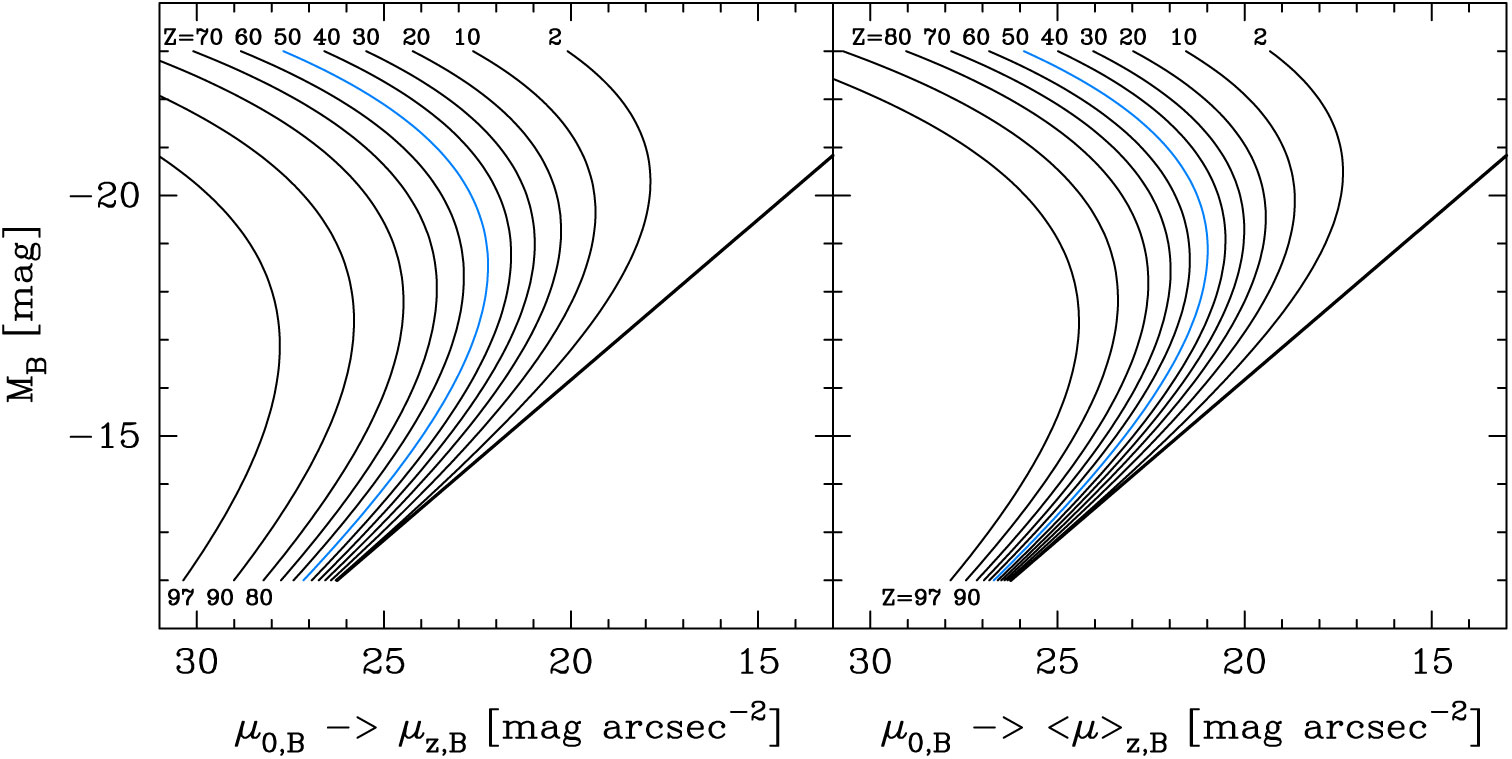
ETG scaling relations between absolute B-band magnitude and the B-band surface brightness at projected radii containing different percentages ( $Z=$
2, 10, 20… 80, 90, 97) of the total light (left panel) and the mean surface brightness within these radii (right panel). The thick straight line is the relation from Figure 1 involving the central surface brightness
$Z=$
2, 10, 20… 80, 90, 97) of the total light (left panel) and the mean surface brightness within these radii (right panel). The thick straight line is the relation from Figure 1 involving the central surface brightness $\mu_{0,B}$
. The curved lines corresponding to
$\mu_{0,B}$
. The curved lines corresponding to $R_{\rm e}$
, that is, the radius enclosing 50% (
$R_{\rm e}$
, that is, the radius enclosing 50% ( $Z=50$
,
$Z=50$
, $z=0.5$
) of the total light, show the behaviour of both the effective surface brightness
$z=0.5$
) of the total light, show the behaviour of both the effective surface brightness $\mu_{\rm e}$
and the mean effective surface brightness
$\mu_{\rm e}$
and the mean effective surface brightness $\langle \mu \rangle_{\rm e}$
. As revealed in Graham (Reference Graham, Oswalt and Keel2013, see his Figures 2–8), the ETGs in Figure 1 follow the
$\langle \mu \rangle_{\rm e}$
. As revealed in Graham (Reference Graham, Oswalt and Keel2013, see his Figures 2–8), the ETGs in Figure 1 follow the $Z=50$
curves shown here. The different absolute magnitude associated with the apparent midpoint or bend in the curves with different values of Z is not due to different formation physics at brighter or fainter magnitudes.
$Z=50$
curves shown here. The different absolute magnitude associated with the apparent midpoint or bend in the curves with different values of Z is not due to different formation physics at brighter or fainter magnitudes.
While the ETG population are unified by the linear $\mathfrak{M}$
–
$\mathfrak{M}$
– $\mu_0$
and
$\mu_0$
and $\mathfrak{M}$
–
$\mathfrak{M}$
– $\log(n)$
relations — with no evidence for a divide at
$\log(n)$
relations — with no evidence for a divide at $\mathfrak{M}_B \approx -18$
mag — the peak in the bend of the (
$\mathfrak{M}_B \approx -18$
mag — the peak in the bend of the ( $z=0.5$
)
$z=0.5$
) $\mathfrak{M}$
–
$\mathfrak{M}$
– $\mu_{\rm e}$
and
$\mu_{\rm e}$
and $\mathfrak{M}$
–
$\mathfrak{M}$
– $\langle \mu \rangle_{\rm e}$
distribution occurs at
$\langle \mu \rangle_{\rm e}$
distribution occurs at $\mathfrak{M}_B \approx -18$
mag. This has contributed to decades of belief that different physical processes have shaped the ETGs brighter and fainter than
$\mathfrak{M}_B \approx -18$
mag. This has contributed to decades of belief that different physical processes have shaped the ETGs brighter and fainter than $\mathfrak{M}_B \approx -18$
mag. However, Figure 3 reveals that had de Vaucouleurs used a radius containing 97% of the total light, then some might today be claiming that the divide between dwarf and ordinary ETGs occurs at
$\mathfrak{M}_B \approx -18$
mag. However, Figure 3 reveals that had de Vaucouleurs used a radius containing 97% of the total light, then some might today be claiming that the divide between dwarf and ordinary ETGs occurs at $\mathfrak{M}_B=-17$
mag; or had de Vaucouleurs used a radius containing 2% of the galaxy’s total light, then they might be advocating for a divide at
$\mathfrak{M}_B=-17$
mag; or had de Vaucouleurs used a radius containing 2% of the galaxy’s total light, then they might be advocating for a divide at $\mathfrak{M}_B=-20.5$
mag.
$\mathfrak{M}_B=-20.5$
mag.
The crucial point is that one should not assign a physical interpretation to the bend. Graham & Guzmán (Reference Graham and Guzmán2003), and Graham (Reference Graham, Oswalt and Keel2013), tried to make this point using only the $Z=50$
curves in Figure 3 and explaining that the bend is due to the light profile shape changing smoothly as the absolute magnitude changes. That is, it is not due to different physical processes operating at absolute magnitudes fainter and brighter than
$Z=50$
curves in Figure 3 and explaining that the bend is due to the light profile shape changing smoothly as the absolute magnitude changes. That is, it is not due to different physical processes operating at absolute magnitudes fainter and brighter than $-18$
mag (or
$-18$
mag (or $-17$
mag or
$-17$
mag or $-20.5$
mag).
$-20.5$
mag).
Despite the above, there has been a remarkable number of claims of supporting evidence for the false divide at $\mathfrak{M}_B \approx -18$
mag. This often pertains to observations that some quantity (e.g. Sérsic index or colour or dynamical mass-to-light ratio) is, on average, different between ETGs brighter and fainter than
$\mathfrak{M}_B \approx -18$
mag. This often pertains to observations that some quantity (e.g. Sérsic index or colour or dynamical mass-to-light ratio) is, on average, different between ETGs brighter and fainter than $\mathfrak{M}_B \approx -18$
mag. This paper has endeavoured to more fully explain the nature of ETGs by including the additional curves in Figure 3 and by revealing in the coming sections what the distribution of ETGs looks like in related diagrams involving effective radii and other measures of radii. There is much that needs addressing given the decades of literature on this subject, the engrained nature of assigning a divide between dwarf and ordinary ETGs at
$\mathfrak{M}_B \approx -18$
mag. This paper has endeavoured to more fully explain the nature of ETGs by including the additional curves in Figure 3 and by revealing in the coming sections what the distribution of ETGs looks like in related diagrams involving effective radii and other measures of radii. There is much that needs addressing given the decades of literature on this subject, the engrained nature of assigning a divide between dwarf and ordinary ETGs at $\mathfrak{M}_B = -18$
mag, and the many (yet to be widely recognised and utilised) insights from understanding these curved scaling relations.
$\mathfrak{M}_B = -18$
mag, and the many (yet to be widely recognised and utilised) insights from understanding these curved scaling relations.
4.1.2. Luminosity-(effective radius) diagram
Due to how the light profile smoothly and systematically changes shape with absolute magnitude (e.g. Fisher & Drory, Reference Fisher and Drory2010, see their Figure 13), when using effective half-light radii ( $z=0.5$
), it results in a distribution of ETGs — and bulges — which is curved (e.g. Lange et al., Reference Lange, Driver and Robotham2015, and references therein). Here, Graham et al. (Reference Graham, Merritt, Moore, Diemand and Terzić2006, see their Figure 1) and Graham & Worley (Reference Graham and Worley2008, see their Figure 11) are expanded upon by additionally showing what the size–luminosity relation looks like when using scale radii that effectively enclose different fractions of the total galaxy light. This also reveals how the absolute magnitude associated with the alleged dichotomy between dwarf (
$z=0.5$
), it results in a distribution of ETGs — and bulges — which is curved (e.g. Lange et al., Reference Lange, Driver and Robotham2015, and references therein). Here, Graham et al. (Reference Graham, Merritt, Moore, Diemand and Terzić2006, see their Figure 1) and Graham & Worley (Reference Graham and Worley2008, see their Figure 11) are expanded upon by additionally showing what the size–luminosity relation looks like when using scale radii that effectively enclose different fractions of the total galaxy light. This also reveals how the absolute magnitude associated with the alleged dichotomy between dwarf ( $\mathfrak{M}_B > -18$
mag) and ordinary (
$\mathfrak{M}_B > -18$
mag) and ordinary ( $\mathfrak{M}_B \lt -18$
mag) ETGs is fictitious, purely dependent on the arbitrary fraction z rather than different physical formation processes.
$\mathfrak{M}_B \lt -18$
mag) ETGs is fictitious, purely dependent on the arbitrary fraction z rather than different physical formation processes.
Building upon equation 12 from Graham & Driver (Reference Graham and Driver2005), which used $R_{\rm e}$
and thus
$R_{\rm e}$
and thus $z=0.5$
, the generalised expression for the total absolute magnitude, in terms of the radius
$z=0.5$
, the generalised expression for the total absolute magnitude, in terms of the radius $R_z$
containing the fraction z of the total light, is given by
$R_z$
containing the fraction z of the total light, is given by
 \begin{equation}
\mathfrak{M}_{\rm tot,B} = \langle\mu\rangle_{\rm z,B} - 2.5\log(\pi R_{\rm z,kpc}^2/z)
- 36.57,
\label{eqn23}
\end{equation}
\begin{equation}
\mathfrak{M}_{\rm tot,B} = \langle\mu\rangle_{\rm z,B} - 2.5\log(\pi R_{\rm z,kpc}^2/z)
- 36.57,
\label{eqn23}
\end{equation}
where $\langle\mu\rangle_{\rm z,B}$
is the mean surface brightness within
$\langle\mu\rangle_{\rm z,B}$
is the mean surface brightness within $R_z$
. This can be rearranged to give the expression
$R_z$
. This can be rearranged to give the expression
 \begin{eqnarray}
\log R_{\rm z,kpc} &=& \frac{\mu_0 - \mathfrak{M}_{\rm tot}}{5} + \frac{\log z - \log[f(n)]}{2}
\nonumber \\ &+& \frac{b_{n,z}}{2\ln(10)} - 7.065,
\label{eqn24}\end{eqnarray}
\begin{eqnarray}
\log R_{\rm z,kpc} &=& \frac{\mu_0 - \mathfrak{M}_{\rm tot}}{5} + \frac{\log z - \log[f(n)]}{2}
\nonumber \\ &+& \frac{b_{n,z}}{2\ln(10)} - 7.065,
\label{eqn24}\end{eqnarray}
where f(n) is given in equation (20). Using equation (17) to replace $\mu_0$
with
$\mu_0$
with $\mathfrak{M}_{\rm tot}$
, this expression becomes
$\mathfrak{M}_{\rm tot}$
, this expression becomes
 \begin{eqnarray}
\log R_{\rm z,kpc} &=& \frac{\mathfrak{M}_{\rm tot}}{10} + \frac{\log z - \log[f(n)]}{2}
\nonumber \\
&+& 0.217b_{n,z} + 1.2874.
\label{eqn25}\end{eqnarray}
\begin{eqnarray}
\log R_{\rm z,kpc} &=& \frac{\mathfrak{M}_{\rm tot}}{10} + \frac{\log z - \log[f(n)]}{2}
\nonumber \\
&+& 0.217b_{n,z} + 1.2874.
\label{eqn25}\end{eqnarray}
The latter term in equation (25), involving z, cancels with the same term in f(n), and thus the dependence of $R_z$
on z occurs via the
$R_z$
on z occurs via the $b_{n,z}$
term (equation (21)).
$b_{n,z}$
term (equation (21)).
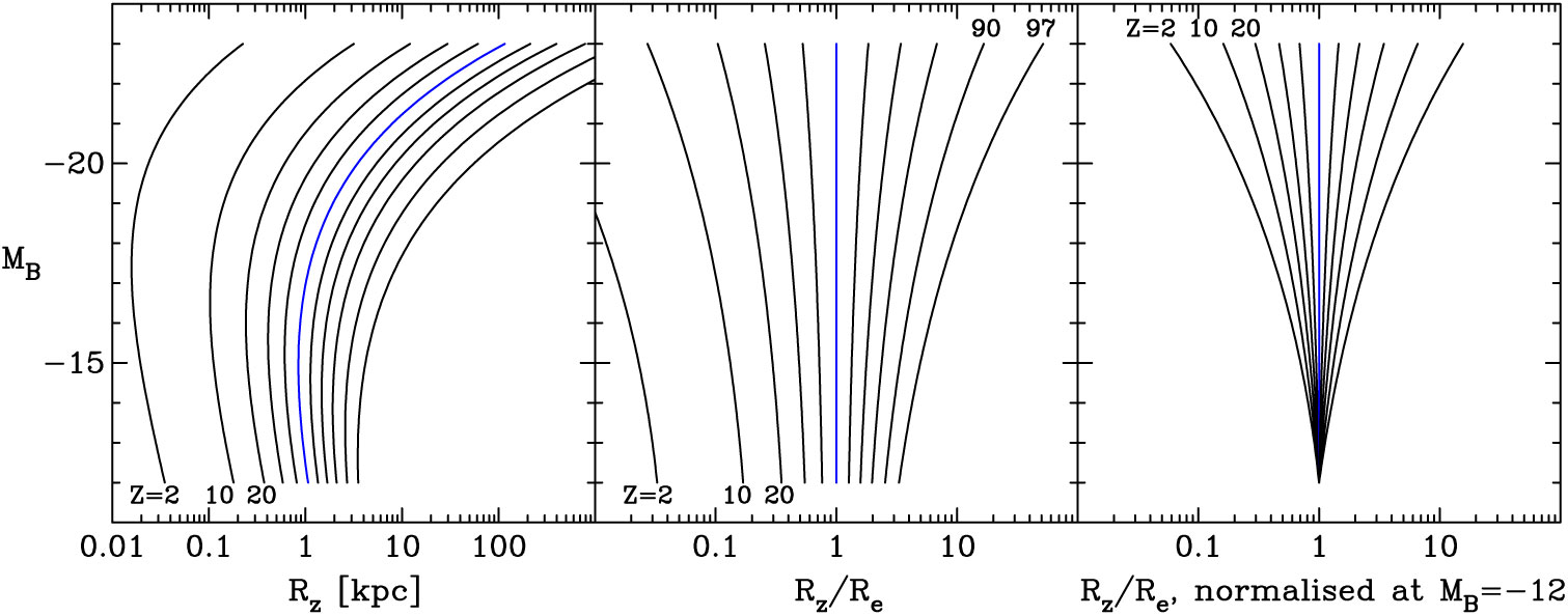
Figure 4 presents the ETG luminosity–size relations for a range of fractions z, expressed there as a percentage Z. The curved behaviour is, once again, due to the ETG population smoothly changing its light profile shape — as quantified by the Sérsic index — with absolute magnitude. It can readily be appreciated that adopting some fixed fraction z, such as 0.5, and then claiming that different physical processes have shaped the luminosity–size relation on either side of the apparent bend-point would be a misleading endeavour (e.g. Fisher & Drory, Reference Fisher and Drory2010, 2016.
As can be seen in the left-hand panel of Figure 4, the bright arm of the curved $\mathfrak{M}_B$
–
$\mathfrak{M}_B$
– $\log R_{\rm e}$
relation for ETGs is approximately linear. This was noted by Fish (Reference Fish1963), who reported
$\log R_{\rm e}$
relation for ETGs is approximately linear. This was noted by Fish (Reference Fish1963), who reported
 $\log L
\propto (1\,{\rm to}\,1.5)\log R_{\rm e}$
or equivalently
$\log L
\propto (1\,{\rm to}\,1.5)\log R_{\rm e}$
or equivalently
 $\mathfrak{M}_p \propto
-(2.5\,{\rm to}\,3.75)\log R_{\rm e}$
, and can be seen in Figure 1 of Sérsic (Reference Sérsic1968b, using the data from Fish, Reference Fish1964; see also Brookes and Rood, Reference Brookes and Rood1971; Gudehus & Hegyi, Reference Gudehus and Hegyi1991; Shen et al., Reference Shen, Mo and White2003; Graham & Worley, Reference Graham and Worley2008; Lange et al., Reference Lange, Driver and Robotham2015)Footnote hFootnote i. Sérsic (Reference Sérsic1968b) was perhaps the first to remark upon the offset nature of the faint ETGs from the bright ETGs in the
$\mathfrak{M}_p \propto
-(2.5\,{\rm to}\,3.75)\log R_{\rm e}$
, and can be seen in Figure 1 of Sérsic (Reference Sérsic1968b, using the data from Fish, Reference Fish1964; see also Brookes and Rood, Reference Brookes and Rood1971; Gudehus & Hegyi, Reference Gudehus and Hegyi1991; Shen et al., Reference Shen, Mo and White2003; Graham & Worley, Reference Graham and Worley2008; Lange et al., Reference Lange, Driver and Robotham2015)Footnote hFootnote i. Sérsic (Reference Sérsic1968b) was perhaps the first to remark upon the offset nature of the faint ETGs from the bright ETGs in the $\mathfrak{M}_B$
–
$\mathfrak{M}_B$
– $\log R_{\rm e}$
diagram. Not understanding the bend in this diagram — referred to as the ‘transition region’ by Sérsic (Reference Sérsic1968b) — coupled with the inclusion of three unusually small galaxies, Sérsic attributed the bend to two populations of (dwarf and giant) elliptical galaxies, rather than one population with smoothly varying properties.
$\log R_{\rm e}$
diagram. Not understanding the bend in this diagram — referred to as the ‘transition region’ by Sérsic (Reference Sérsic1968b) — coupled with the inclusion of three unusually small galaxies, Sérsic attributed the bend to two populations of (dwarf and giant) elliptical galaxies, rather than one population with smoothly varying properties.
Left panel: relations describing the distribution of ETG B-band absolute magnitude versus the projected radii enclosing various percentages ( $Z=$
2, 10, 20… 80, 90, 97) of their total flux (equation (25)). The relation involving the effective half-light radius corresponds to the
$Z=$
2, 10, 20… 80, 90, 97) of their total flux (equation (25)). The relation involving the effective half-light radius corresponds to the $Z=50$
curve. Middle and right panels: It can be seen how much the scale radii vary depending on the arbitrary percentage of light used to define them.
$Z=50$
curve. Middle and right panels: It can be seen how much the scale radii vary depending on the arbitrary percentage of light used to define them.
Confounding the situation further, Sérsic added LTGs into his $\mathfrak{M}_p$
–
$\mathfrak{M}_p$
– $\log R_{\rm e}$
diagram (see his Figure 2; cf. Figures 9 and 14 from Cappellari et al., Reference Cappellari, McDermid and Alatalo2013b). Involving
$\log R_{\rm e}$
diagram (see his Figure 2; cf. Figures 9 and 14 from Cappellari et al., Reference Cappellari, McDermid and Alatalo2013b). Involving $R_{\rm e}$
measures from both two-dimensional spirals and three-dimensional ellipticals, Sérsic (Reference Sérsic1968b) observed a slight overlap and wrote that ‘it seems difficult to deny the existence of the sequence of irregulars and spirals joining that of the ellipticals in the transition region’. Kormendy (Reference Kormendy1985) adopted this same practice.
$R_{\rm e}$
measures from both two-dimensional spirals and three-dimensional ellipticals, Sérsic (Reference Sérsic1968b) observed a slight overlap and wrote that ‘it seems difficult to deny the existence of the sequence of irregulars and spirals joining that of the ellipticals in the transition region’. Kormendy (Reference Kormendy1985) adopted this same practice.
For $R_{\rm e} \mathbin{\lower.3ex\hbox{$\buildrel\gt\over
{\smash{\scriptstyle\sim}\vphantom{_x}}$}} $
1–2 kpc and a photographic absolute magnitude
$R_{\rm e} \mathbin{\lower.3ex\hbox{$\buildrel\gt\over
{\smash{\scriptstyle\sim}\vphantom{_x}}$}} $
1–2 kpc and a photographic absolute magnitude $\mathfrak{M}_p$
brighter than
$\mathfrak{M}_p$
brighter than $-19.5$
magFootnote j, Sérsic (Reference Sérsic1968b) fit a line with a slope of unity to the distribution of giant elliptical galaxies in his (
$-19.5$
magFootnote j, Sérsic (Reference Sérsic1968b) fit a line with a slope of unity to the distribution of giant elliptical galaxies in his ( $\log {\rm Mass}$
)–(
$\log {\rm Mass}$
)–( $\log R_{\rm e}$
) diagram. This distribution resembled that in his
$\log R_{\rm e}$
) diagram. This distribution resembled that in his $\mathfrak{M}$
–
$\mathfrak{M}$
– $\log R_{\rm e}$
diagram because he claims to have used a constant mass-to-light ratio of 30. As such, Sérsic (Reference Sérsic1968b) reported a distribution in which the absolute magnitude scaled as
$\log R_{\rm e}$
diagram because he claims to have used a constant mass-to-light ratio of 30. As such, Sérsic (Reference Sérsic1968b) reported a distribution in which the absolute magnitude scaled as $-2.5\log R_{\rm e}$
. Given that the magnitude of a galaxy is proportional to
$-2.5\log R_{\rm e}$
. Given that the magnitude of a galaxy is proportional to $\langle \mu \rangle_{\rm e} - 5\log R_{\rm e}$
(e.g. de Vaucouleurs & Page, Reference de Vaucouleurs and Page1962, see their equation 6), one immediately has the relation
$\langle \mu \rangle_{\rm e} - 5\log R_{\rm e}$
(e.g. de Vaucouleurs & Page, Reference de Vaucouleurs and Page1962, see their equation 6), one immediately has the relation $\langle \mu \rangle_{\rm e} \propto 2.5\log R_{\rm e}$
for the distribution of giant elliptical galaxies. Furthermore, given that
$\langle \mu \rangle_{\rm e} \propto 2.5\log R_{\rm e}$
for the distribution of giant elliptical galaxies. Furthermore, given that $\mu_{\rm e} - \langle \mu \rangle_{\rm e} = 1.393$
for the
$\mu_{\rm e} - \langle \mu \rangle_{\rm e} = 1.393$
for the $R^{1/4}$
model that Sérsic (Reference Sérsic1968b) was using, one also immediately has that
$R^{1/4}$
model that Sérsic (Reference Sérsic1968b) was using, one also immediately has that $\mu_{\rm e} \propto 2.5\log R_{\rm e}$
. This can be compared with Kormendy (Reference Kormendy1977)Footnote k who reported
$\mu_{\rm e} \propto 2.5\log R_{\rm e}$
. This can be compared with Kormendy (Reference Kormendy1977)Footnote k who reported
 $\mu_{\rm e} \propto
3.02\log R_{\rm e}$
.
$\mu_{\rm e} \propto
3.02\log R_{\rm e}$
.
Somerville & Davé (Reference Somerville and Davé2015, see their Section 1.1.4) refer to the ( $\log {\rm Mass}$
)–(
$\log {\rm Mass}$
)–( $\log R_{\rm e}$
) relation as the Kormendy relation (see also Cappellari, Reference Cappellari2016, his Section 4.1.1), but it would be more appropriate if that title was assigned to the linear relation which Kormendy fit to the bright arm of what we now know is the curved
$\log R_{\rm e}$
) relation as the Kormendy relation (see also Cappellari, Reference Cappellari2016, his Section 4.1.1), but it would be more appropriate if that title was assigned to the linear relation which Kormendy fit to the bright arm of what we now know is the curved $\mu_{\rm e}$
–
$\mu_{\rm e}$
– $\log R_{\rm e}$
relation, and to instead refer to the linear (
$\log R_{\rm e}$
relation, and to instead refer to the linear ( $\log {\rm Mass}$
)–(
$\log {\rm Mass}$
)–( $\log R_{\rm e}$
) and
$\log R_{\rm e}$
) and $\mathfrak{M}$
–(
$\mathfrak{M}$
–( $\log R_{\rm e}$
) relations used to describe the distribution of bright elliptical galaxies as the FishFootnote l or Fish–Sérsic relation. The curved
$\log R_{\rm e}$
) relations used to describe the distribution of bright elliptical galaxies as the FishFootnote l or Fish–Sérsic relation. The curved $\mu_{\rm e}$
–
$\mu_{\rm e}$
– $\log R_{\rm e}$
relation is explored in 4.1.3.
$\log R_{\rm e}$
relation is explored in 4.1.3.
Three additional insights from Figure 4 can readily be made. The first has implications for dark matter (Kent, Reference Kent1990, and references therein) if using $\sigma^2R_{\rm e}$
(e.g. Poincare & Vergne, Reference Poincare and Vergne1911; Poveda, Reference Poveda1958, Reference Poveda1961) as a proxy for massFootnote m in a population of ETGs with a range of absolute magnitudes and thus a range of light profile shapes. Considering how the ratio of radii (
$\sigma^2R_{\rm e}$
(e.g. Poincare & Vergne, Reference Poincare and Vergne1911; Poveda, Reference Poveda1958, Reference Poveda1961) as a proxy for massFootnote m in a population of ETGs with a range of absolute magnitudes and thus a range of light profile shapes. Considering how the ratio of radii ( $R_{z_1}/R_{z_2}$
) at fixed absolute magnitude changes, for different values of
$R_{z_1}/R_{z_2}$
) at fixed absolute magnitude changes, for different values of $z_1$
and
$z_1$
and $z_2$
in Figure 4, one should pause for thought when using effective half-light radii (
$z_2$
in Figure 4, one should pause for thought when using effective half-light radii ( $z=0.5$
) to measure dynamical (stellar plus dark matter) masses via the proportionality
$z=0.5$
) to measure dynamical (stellar plus dark matter) masses via the proportionality $\sigma^2 R_{\rm e}$
(e.g. Drory, Bender, & Hopp Reference Drory, Bender and Hopp2004, see their Figure 3; Cappellari et al., Reference Cappellari, Bacon and Bureau2006 who use the luminosity-weighted
$\sigma^2 R_{\rm e}$
(e.g. Drory, Bender, & Hopp Reference Drory, Bender and Hopp2004, see their Figure 3; Cappellari et al., Reference Cappellari, Bacon and Bureau2006 who use the luminosity-weighted $\sigma$
values within half-light radii determined from
$\sigma$
values within half-light radii determined from $R^{1/4}$
models; Cappellari et al., Reference Cappellari, Scott and Alatalo2013a). Using
$R^{1/4}$
models; Cappellari et al., Reference Cappellari, Scott and Alatalo2013a). Using $\sigma^2R_z$
, with
$\sigma^2R_z$
, with $z\ne0.5$
, will produce a different trend because the ratio
$z\ne0.5$
, will produce a different trend because the ratio $R_{\rm e}/R_z$
is not constant for different
$R_{\rm e}/R_z$
is not constant for different $\mathfrak{M}_B$
(see also the telling merger simulations by Farouki et al., Reference Farouki, Shapiro and Duncan1983 revealing how
$\mathfrak{M}_B$
(see also the telling merger simulations by Farouki et al., Reference Farouki, Shapiro and Duncan1983 revealing how $R_{10}/R_{\rm e}$
changes with mass, and the work by Campbell et al., Reference Campbell, Frenk and Jenkins2017 and Lyskova et al., Reference Lyskova, Thomas, Churazov, Tremaine and Naab2015). Therefore, it may not be appropriate to solely invoke varying fractions of dark matter to explain the systematic differences, as a function of varying absolute magnitude, between (i) this dynamical mass estimate (based on the arbitrary radius
$R_{10}/R_{\rm e}$
changes with mass, and the work by Campbell et al., Reference Campbell, Frenk and Jenkins2017 and Lyskova et al., Reference Lyskova, Thomas, Churazov, Tremaine and Naab2015). Therefore, it may not be appropriate to solely invoke varying fractions of dark matter to explain the systematic differences, as a function of varying absolute magnitude, between (i) this dynamical mass estimate (based on the arbitrary radius $R_{\rm e}$
) and (ii) the stellar mass estimate (obtained from the absolute magnitude). This will be broached in a subsequent study, covering the ‘Fundamental Plane’ (Djorgovski and Davis, Reference Djorgovski and Davis1987), improved planes, and implications for both dark matter estimates (e.g. Graves & Faber, Reference Graves and Faber2010) and ETG formation (see Cappellari, Reference Cappellari2016, his Section 4, for an overview).
$R_{\rm e}$
) and (ii) the stellar mass estimate (obtained from the absolute magnitude). This will be broached in a subsequent study, covering the ‘Fundamental Plane’ (Djorgovski and Davis, Reference Djorgovski and Davis1987), improved planes, and implications for both dark matter estimates (e.g. Graves & Faber, Reference Graves and Faber2010) and ETG formation (see Cappellari, Reference Cappellari2016, his Section 4, for an overview).
Second, it is noted that the acceleration at some radius R, inside a symmetrical pressure supported system with velocity dispersion $\sigma$
, is proportional to
$\sigma$
, is proportional to $GM/R^2$
or
$GM/R^2$
or $\sigma^2/R$
. Due to the structural non-homology of ETGs, this ratio will vary with M in different ways depending on what fraction z has been used to measure R. This has relevance to the critical acceleration parameter
$\sigma^2/R$
. Due to the structural non-homology of ETGs, this ratio will vary with M in different ways depending on what fraction z has been used to measure R. This has relevance to the critical acceleration parameter $a_0$
, or characteristic surface density
$a_0$
, or characteristic surface density $M/R^2$
, in modified Newtonian dynamics (Milgrom, Reference Milgrom1983; Sanders & McGaugh, Reference Sanders and McGaugh2002, see their Figure 7; Milgrom & Sanders, Reference Milgrom and Sanders2003; Kroupa et al., Reference Kroupa, Famaey and de Boer2010, their Figure 7; Misgeld & Hilker, Reference Misgeld and Hilker2011, their Figure 7; Famaey & McGaugh, Reference Famaey and McGaugh2012).
$M/R^2$
, in modified Newtonian dynamics (Milgrom, Reference Milgrom1983; Sanders & McGaugh, Reference Sanders and McGaugh2002, see their Figure 7; Milgrom & Sanders, Reference Milgrom and Sanders2003; Kroupa et al., Reference Kroupa, Famaey and de Boer2010, their Figure 7; Misgeld & Hilker, Reference Misgeld and Hilker2011, their Figure 7; Famaey & McGaugh, Reference Famaey and McGaugh2012).
Third, it may also be insightful to explore the near-constant $R_{\rm e,bulge}/h_{\rm disc}$
ratio of
$R_{\rm e,bulge}/h_{\rm disc}$
ratio of $\sim$
0.2 observed in spiral galaxies (e.g. Courteau et al., Reference Courteau, de Jong and Broeils1996; Graham & Worley, Reference Graham and Worley2008, and references therein), which appears irrespective of whether the bulge is considered to be a ‘classical’ bulge or a ‘pseudobulge’. For instance, the use of
$\sim$
0.2 observed in spiral galaxies (e.g. Courteau et al., Reference Courteau, de Jong and Broeils1996; Graham & Worley, Reference Graham and Worley2008, and references therein), which appears irrespective of whether the bulge is considered to be a ‘classical’ bulge or a ‘pseudobulge’. For instance, the use of $z=0.1$
or
$z=0.1$
or $z=0.9$
, rather than
$z=0.9$
, rather than $z=0.5$
, is expected to result in this ratio systematically changing, with magnitude, by a factor of
$z=0.5$
, is expected to result in this ratio systematically changing, with magnitude, by a factor of $\sim$
3 for spiral galaxies.
$\sim$
3 for spiral galaxies.
4.1.3. (Effective radius)-(effective surface brightness) diagram
In addition to the $R_{\rm e}$
–
$R_{\rm e}$
– $\mu_{\rm e}$
and
$\mu_{\rm e}$
and $R_{\rm e}$
–
$R_{\rm e}$
–
 $\langle \mu
\rangle_{\rm e}$
distributions (derived using
$\langle \mu
\rangle_{\rm e}$
distributions (derived using $z=0.5$
), it is instructive to show the size-(surface brightness) distributions
$z=0.5$
), it is instructive to show the size-(surface brightness) distributions $R_z$
–
$R_z$
– $\mu_z$
and
$\mu_z$
and $R_z$
–
$R_z$
– $\langle \mu \rangle_z$
that one would obtain for different values of z, corresponding to the fraction of light contained within
$\langle \mu \rangle_z$
that one would obtain for different values of z, corresponding to the fraction of light contained within $R_z$
. Figure 5 reveals a number of things, three of which are worth explicitly pointing out here, while many other important but less-recognised aspects will be saved for a follow-up paper pertaining to both understanding the ‘Fundamental Plane’ and constructing an improved plane/surface.
$R_z$
. Figure 5 reveals a number of things, three of which are worth explicitly pointing out here, while many other important but less-recognised aspects will be saved for a follow-up paper pertaining to both understanding the ‘Fundamental Plane’ and constructing an improved plane/surface.
Size–(surface brightness) relations — describing the distribution of galaxies having a range of B-band absolute magnitudes (from $-12$
to
$-12$
to $-23$
mag) — based on projected radii,
$-23$
mag) — based on projected radii, $R_z$
, enclosing different percentages (
$R_z$
, enclosing different percentages ( $Z=$
5, 10, 20… 80, 90, 95) of the galaxy light. The innermost curve is associated with the 50% radius, known as the effective half-light radius
$Z=$
5, 10, 20… 80, 90, 95) of the galaxy light. The innermost curve is associated with the 50% radius, known as the effective half-light radius $R_{\rm e}$
, the effective surface brightness
$R_{\rm e}$
, the effective surface brightness $\mu_{\rm e}$
at this radius (left panel), and the average surface brightness
$\mu_{\rm e}$
at this radius (left panel), and the average surface brightness $\langle \mu \rangle_{\rm e}$
within this radius (right panel). The upper envelope in the left-hand panel has a slope of
$\langle \mu \rangle_{\rm e}$
within this radius (right panel). The upper envelope in the left-hand panel has a slope of $\sim$
3.5, while the upper envelope in the right-hand panel has a slope of
$\sim$
3.5, while the upper envelope in the right-hand panel has a slope of $\sim$
2.8.
$\sim$
2.8.
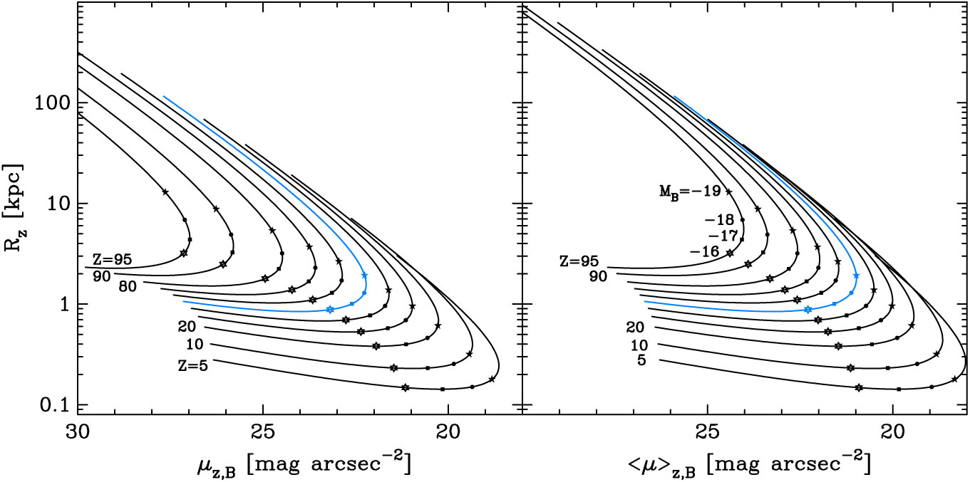
First, had the community been using radii enclosing 95% or 5% of the total light, then those interpreting the bend in the corresponding size-(surface brightness) diagram may likely be claiming evidence of distinctly different formation physics for galaxies brighter and fainter than $\sim -16.5$
mag or
$\sim -16.5$
mag or $\sim -19.5$
mag, respectively.
$\sim -19.5$
mag, respectively.
Second, the bunching up of tracks in the top right of Figure 5 reveals why the $R_{\rm e}$
–
$R_{\rm e}$
– $\mu_{\rm e}$
and
$\mu_{\rm e}$
and $R_{\rm e}$
–
$R_{\rm e}$
–
 $\langle \mu
\rangle_{\rm e}$
relations have a low level of scatter for ETGs with B-band absolute magnitudes brighter than
$\langle \mu
\rangle_{\rm e}$
relations have a low level of scatter for ETGs with B-band absolute magnitudes brighter than $\approx -19$
mag. If one mis-measures the half-light radius and instead captures the radius enclosing 20, 30, 40, 60, 70, or 80% of the total light, the surface brightness terms associated with these radii are such that the galaxy’s location in the
$\approx -19$
mag. If one mis-measures the half-light radius and instead captures the radius enclosing 20, 30, 40, 60, 70, or 80% of the total light, the surface brightness terms associated with these radii are such that the galaxy’s location in the $R_{\rm e}$
–
$R_{\rm e}$
– $\mu_{\rm e}$
diagram moves along the upper envelope seen in Figure 5 and thereby maintains a tight
$\mu_{\rm e}$
diagram moves along the upper envelope seen in Figure 5 and thereby maintains a tight $R_{\rm e}$
–
$R_{\rm e}$
– $\mu_{\rm e}$
relation.
$\mu_{\rm e}$
relation.
Third, the inclusion of ETGs fainter than $\mathfrak{M}_B \approx -19$
mag results in a thickening of the distribution in the
$\mathfrak{M}_B \approx -19$
mag results in a thickening of the distribution in the $R_{\rm e}$
–
$R_{\rm e}$
– $\mu_{\rm e}$
diagram (e.g. Kodaira, Okamura, & Watanabe, Reference Kodaira, Okamura and Watanabe1983; Capaccioli, Caon, & D’Onofrio, Reference Capaccioli, Caon and D’Onofrio1994) as mis-measures of the half-light radius will shift galaxies perpendicular to the curved
$\mu_{\rm e}$
diagram (e.g. Kodaira, Okamura, & Watanabe, Reference Kodaira, Okamura and Watanabe1983; Capaccioli, Caon, & D’Onofrio, Reference Capaccioli, Caon and D’Onofrio1994) as mis-measures of the half-light radius will shift galaxies perpendicular to the curved $z=0.5$
relation at faint absolute magnitudes.
$z=0.5$
relation at faint absolute magnitudes.
Bildfell et al. (Reference Bildfell, Hoekstra, Babul and Mahdavi2008) report that ‘The Kormendy relation of our BCGs is steeper than that of the [less luminous] local ellipticals, suggesting differences in the assembly history of these types of systems’. Although the literature is full of similar claims, such interpretations are not appropriate given the curved $R_{\rm e}$
–
$R_{\rm e}$
– $\mu_{\rm e}$
relation’s dependence on the arbitrary value
$\mu_{\rm e}$
relation’s dependence on the arbitrary value $z=0.5$
. Countless studies which have attached a physical significance to slopes and bends in scaling diagrams involving the logarithm of
$z=0.5$
. Countless studies which have attached a physical significance to slopes and bends in scaling diagrams involving the logarithm of $R_{\rm e}$
,
$R_{\rm e}$
, $\mu_{\rm e}$
, and/or
$\mu_{\rm e}$
, and/or $\langle \mu \rangle _{\rm e}$
should be questioned. As already noted in Graham & Guzman (2004) and Graham (2005), this remark extends to studies of the ‘Fundamental Plane’ (Guzmán et al. 2019, in preparation).
$\langle \mu \rangle _{\rm e}$
should be questioned. As already noted in Graham & Guzman (2004) and Graham (2005), this remark extends to studies of the ‘Fundamental Plane’ (Guzmán et al. 2019, in preparation).
A range of other measures for galaxy size is explored in the remainder of this section.
4.2. An alternative scheme for defining projected radii
The previous text focused on projected radii that enclosed an arbitrary fraction of light relative to the light enclosed within a radius of infinity, that is, the total light. One can, alternatively, define a radius where the intensity is an arbitrary fraction of the intensity at $R=0$
. In the case of the exponential galaxy light profile model, the parameter h denotes the scale length where the intensity has dropped by a factor of
$R=0$
. In the case of the exponential galaxy light profile model, the parameter h denotes the scale length where the intensity has dropped by a factor of ${\rm e}\approx2.718$
. This subsection explores radii where the intensity of the
${\rm e}\approx2.718$
. This subsection explores radii where the intensity of the $R^{1/n}$
model has dropped by fixed amounts, effectively replacing the variable
$R^{1/n}$
model has dropped by fixed amounts, effectively replacing the variable ${\rm e}^{b_n}$
term in equation (13) with a constant.
${\rm e}^{b_n}$
term in equation (13) with a constant.
For de Vaucouleurs’ $R^{1/4}$
model (equation (1)), it was noted that the intensity at
$R^{1/4}$
model (equation (1)), it was noted that the intensity at $R_{\rm e}$
is e
$R_{\rm e}$
is e $^{7.669} \approx 2141$
times fainter than the intensity at
$^{7.669} \approx 2141$
times fainter than the intensity at $R=0$
. This corresponds to a surface brightness which is 8.327 mag arcsec-2 fainter than the central surface brightness. It is informative to explore what the size–luminosity diagram looks like when using this alternative, but equally valid, measure of ETG size, that is, the radius where the surface brightness has dropped by a constant 8.327 mag arcsec-2. This is done in Figure 6, where a few other constant values are also used.
$R=0$
. This corresponds to a surface brightness which is 8.327 mag arcsec-2 fainter than the central surface brightness. It is informative to explore what the size–luminosity diagram looks like when using this alternative, but equally valid, measure of ETG size, that is, the radius where the surface brightness has dropped by a constant 8.327 mag arcsec-2. This is done in Figure 6, where a few other constant values are also used.
Left panel: Relations between the absolute B-band magnitude, $\mathfrak{M}_B$
, and the radius where the associated light profile’s surface brightness has dropped by a fixed amount from the central
$\mathfrak{M}_B$
, and the radius where the associated light profile’s surface brightness has dropped by a fixed amount from the central $R=0$
value
$R=0$
value $\mu_0$
(equation (17)).of the Sérsic model having a Sérsic index n dictated by the value of
$\mu_0$
(equation (17)).of the Sérsic model having a Sérsic index n dictated by the value of $\mathfrak{M}_B$
(equation (16)). The leftmost curve in each panel shows the result when using
$\mathfrak{M}_B$
(equation (16)). The leftmost curve in each panel shows the result when using $\Delta\mu=8.327$
mag arcsec-2, which is the difference in surface brightness between
$\Delta\mu=8.327$
mag arcsec-2, which is the difference in surface brightness between $\mu_0$
and
$\mu_0$
and $\mu_{\rm e}$
of de Vaucouleurs’
$\mu_{\rm e}$
of de Vaucouleurs’ $R^{1/4}$
model. Middle panel: Similar, except that the radii shown here denote where the surface brightness profile has dropped by the same set of constant values used in the left panel, but now starting from
$R^{1/4}$
model. Middle panel: Similar, except that the radii shown here denote where the surface brightness profile has dropped by the same set of constant values used in the left panel, but now starting from $R=0.01$
kpc rather than from
$R=0.01$
kpc rather than from $R=0$
. This helps to bypass the rapidly rising inner light profile of systems with high values of n, but which typically contain depleted cores. Right panel: Similar to the middle panel but starting from
$R=0$
. This helps to bypass the rapidly rising inner light profile of systems with high values of n, but which typically contain depleted cores. Right panel: Similar to the middle panel but starting from $R=0.1$
kpc.
$R=0.1$
kpc.
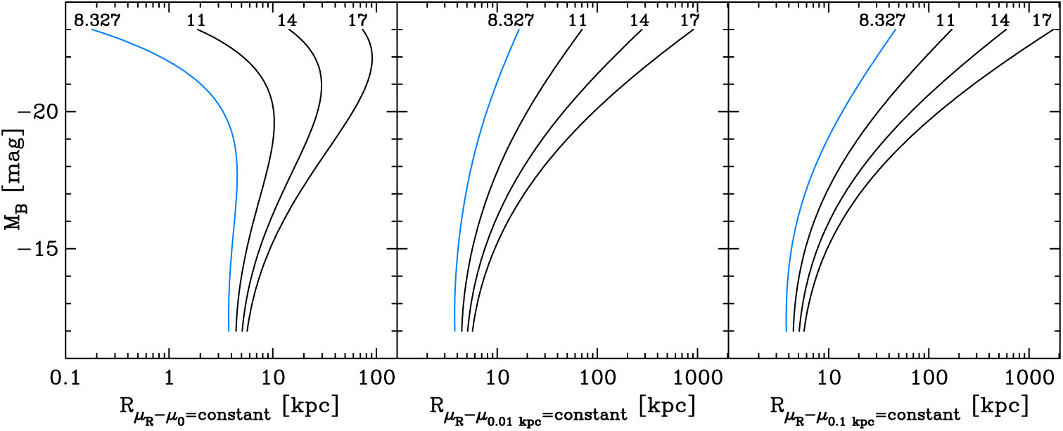
The left panel of Figure 6 reveals little evidence for a divide at $\mathfrak{M}_B \approx -18$
mag between the so-called dwarf and ordinary ETGs. Had astronomers used the above system of radii, calibrated to the Sérsic model’s central surface brightness (at
$\mathfrak{M}_B \approx -18$
mag between the so-called dwarf and ordinary ETGs. Had astronomers used the above system of radii, calibrated to the Sérsic model’s central surface brightness (at $R=0$
), rather than calibrated to the Sérsic model’s total luminosity (at
$R=0$
), rather than calibrated to the Sérsic model’s total luminosity (at $R=\infty$
), then they might well have concluded that there is a dichotomy between bright and faint ETGs at
$R=\infty$
), then they might well have concluded that there is a dichotomy between bright and faint ETGs at
 $\mathfrak{M}_B \approx
-20$
mag and speculated that different physical processes must be responsible for the formation of ETGs fainter and brighter than this absolute magnitude. Some astronomers may have even heralded the observation of partially depleted cores in ETGs more luminous than
$\mathfrak{M}_B \approx
-20$
mag and speculated that different physical processes must be responsible for the formation of ETGs fainter and brighter than this absolute magnitude. Some astronomers may have even heralded the observation of partially depleted cores in ETGs more luminous than $\mathfrak{M}_B \sim -20.5\pm1$
mag — thought to have formed their spheroids from major dry merger events — as the explanation for the bend seen in this alternative luminosity–size diagram.
$\mathfrak{M}_B \sim -20.5\pm1$
mag — thought to have formed their spheroids from major dry merger events — as the explanation for the bend seen in this alternative luminosity–size diagram.
In case some readers might be entertaining the $\Delta\mu=8.327$
mag arcsec-2 curve in the left-hand panel of Figure 6 as evidence for a division at
$\Delta\mu=8.327$
mag arcsec-2 curve in the left-hand panel of Figure 6 as evidence for a division at $\mathfrak{M}_B \approx -20$
mag, additional measures of radii based on larger differences in surface brightness from the central surface brightness have been included. One can see that the location of the bend in the scaling relations shifts from a B-band magnitude of roughly
$\mathfrak{M}_B \approx -20$
mag, additional measures of radii based on larger differences in surface brightness from the central surface brightness have been included. One can see that the location of the bend in the scaling relations shifts from a B-band magnitude of roughly $-20$
to
$-20$
to $-22$
mag as one samples more of the galaxy light. Once again, this demonstrates that these bends are not revealing the existence of different physical processes operating at magnitudes brighter and fainter than the location of the bend. The whip around to smaller radii seen at bright magnitudes in the left-hand panel of Figure 6 is due to the rapidly rising (with decreasing radii), inner light profile of systems with high Sérsic indices. One can devise schemes to circumvent this (see the middle and right-hand panels), which may be desirable given the partially depleted cores in these galaxies which prevent such bright
$-22$
mag as one samples more of the galaxy light. Once again, this demonstrates that these bends are not revealing the existence of different physical processes operating at magnitudes brighter and fainter than the location of the bend. The whip around to smaller radii seen at bright magnitudes in the left-hand panel of Figure 6 is due to the rapidly rising (with decreasing radii), inner light profile of systems with high Sérsic indices. One can devise schemes to circumvent this (see the middle and right-hand panels), which may be desirable given the partially depleted cores in these galaxies which prevent such bright $\mu_0$
values actually being realised. The monotonic size–luminosity relations in Figure 6, which do not use radii where the intensity has dropped by systematically different amounts as a function of luminosity (as occurs with
$\mu_0$
values actually being realised. The monotonic size–luminosity relations in Figure 6, which do not use radii where the intensity has dropped by systematically different amounts as a function of luminosity (as occurs with $R_{\rm e}$
and
$R_{\rm e}$
and $R_z$
) reveal no grounds for segregating dwarf and giant ETGs at
$R_z$
) reveal no grounds for segregating dwarf and giant ETGs at $\mathfrak{M}_B \approx -18$
mag.
$\mathfrak{M}_B \approx -18$
mag.
The middle and right-hand panels of Figure 6 show the distribution of ETG sizes where their surface brightness profiles have dropped by the same values as those used in the left-hand panel, but starting the drop from a radius of 0.01 and 0.1 kpc, rather than from the central value.
4.3. Isophotal radii
Based on isophotal radii, the luminosity–size relation for ETGs was initially considered to be log-linear, that is, linear in log space, unifying dwarf and giant ETGs (e.g. Heidmann, Reference Heidmann1967, Reference Heidmann1969; Holmberg, Reference Holmberg1969; Oemler, Reference Oemler1976; Strom & Strom, Reference Strom and Strom1978), and it largely still is (e.g. Forbes et al., Reference Forbes, Lasky, Graham and Spitler2008, see their Figure 3; van den Bergh, Reference van den Bergh2008; Nair, van den Bergh, & Abraham, Reference Nair, van den Bergh and Abraham2011). This section would therefore be somewhat incomplete if it did not include isophotal radii.
Using a photographic (Pg, i.e. blue filter, Vega mag system) surface brightness of 26.5 mag arcsec-2 to define galaxy diameters, Holmberg (Holmberg, Reference Holmberg1969, see his Figure 9) reported a linear relation, with a slope of $-6$
, between the absolute magnitude and the logarithm of the isophotal major axis diameterFootnote n. Using the major axis diameter of the isophote corresponding to a photographic surface brightness of 25 (Vega) mag arcsec-2, Heidmann, (Reference Heidmann1967, Reference Heidmann1969: see also Fraser, Reference Fraser1977 and Bigay & Paturel, Reference Bigay and Paturel1980) obtained a less steep slope of
$-6$
, between the absolute magnitude and the logarithm of the isophotal major axis diameterFootnote n. Using the major axis diameter of the isophote corresponding to a photographic surface brightness of 25 (Vega) mag arcsec-2, Heidmann, (Reference Heidmann1967, Reference Heidmann1969: see also Fraser, Reference Fraser1977 and Bigay & Paturel, Reference Bigay and Paturel1980) obtained a less steep slope of $-4.75$
for ETGsFootnote o in the
$-4.75$
for ETGsFootnote o in the $\mathfrak{M}$
–(
$\mathfrak{M}$
–( $\log R_{\rm iso}$
) diagram, which he reported as a slope of 1.9 in the
$\log R_{\rm iso}$
) diagram, which he reported as a slope of 1.9 in the $\log L$
–
$\log L$
– $\log R_{\rm iso}$
diagram.
$\log R_{\rm iso}$
diagram.
Some half a century later, using the semimajor axis radius of the 3.6 $\mu$
m isophote whose surface brightness equals 25.5 (AB) mag arcsec-2, Muñoz-Mateos et al. (Reference Muñoz-Mateos, Sheth and Regan2015, see their Figure 14) presented a log-linear radius–(stellar mass) relation for different morphological types. The bright ETGs have the same slope as reported by Heidmann, with
$\mu$
m isophote whose surface brightness equals 25.5 (AB) mag arcsec-2, Muñoz-Mateos et al. (Reference Muñoz-Mateos, Sheth and Regan2015, see their Figure 14) presented a log-linear radius–(stellar mass) relation for different morphological types. The bright ETGs have the same slope as reported by Heidmann, with
 $\log M \propto
(1.9\pm0.1)\log R_{3.6\mu {\rm m}=25.5}$
. Approximating the low-luminosity end of the moderately curved L–
$\log M \propto
(1.9\pm0.1)\log R_{3.6\mu {\rm m}=25.5}$
. Approximating the low-luminosity end of the moderately curved L– $R_{\rm iso}$
relation with a power-law, the faint ETGs in Muñoz-Mateos et al. roughly follow a relation with a slope of
$R_{\rm iso}$
relation with a power-law, the faint ETGs in Muñoz-Mateos et al. roughly follow a relation with a slope of $2.7\pm0.2$
. Muñoz-Mateos et al. additionally show, in their Figure 15, that the use of
$2.7\pm0.2$
. Muñoz-Mateos et al. additionally show, in their Figure 15, that the use of $R_{\rm e}$
, rather than isophotal radii, results in the strongly curved size–luminosity relation seen in Figure 4.
$R_{\rm e}$
, rather than isophotal radii, results in the strongly curved size–luminosity relation seen in Figure 4.
Figure 7 reveals what the size–luminosity relation for ETGs looks like when using six different isophotal radii (specifically, those radii where the B-band surface brightness equals 25, 26, … 30 mag arcsec-2) and using the total B-band absolute magnitude $\mathfrak{M}_B$
within a radius of infinite aperture. The smoothly changing slope is consistent with the slight curve observed for 50 years in magnitude-(isophotal radii) diagrams. For example, as noted above, a moderate change in slope is seen among the ETGs in the
$\mathfrak{M}_B$
within a radius of infinite aperture. The smoothly changing slope is consistent with the slight curve observed for 50 years in magnitude-(isophotal radii) diagrams. For example, as noted above, a moderate change in slope is seen among the ETGs in the $\log \mathfrak{M}$
–
$\log \mathfrak{M}$
– $\log R_{3.6\mu {\rm m}=25.5}$
diagram of Muñoz-Mateos et al. (Reference Muñoz-Mateos, Sheth and Regan2015) at 4–6 kpc. This can be understood in terms of the Sérsic index varying with absolute magnitude, which gives rise to the curves in Figure 7. Although it should be noted that the mapping between Figure 14 in Muñoz-Mateos et al. (Reference Muñoz-Mateos, Sheth and Regan2015) and Figure 7 shown here is not linear because of the colour–magnitude relation for ETGs (e.g. Ferrarese et al., Reference Ferrarese, Côté and Jordán2006, see their Figure 123), in which fainter ETGs are bluer than luminous ETGs. To help anyone who may wish to explore this further, it is quickly noted that given that luminous ETGs have a (
$\log R_{3.6\mu {\rm m}=25.5}$
diagram of Muñoz-Mateos et al. (Reference Muñoz-Mateos, Sheth and Regan2015) at 4–6 kpc. This can be understood in terms of the Sérsic index varying with absolute magnitude, which gives rise to the curves in Figure 7. Although it should be noted that the mapping between Figure 14 in Muñoz-Mateos et al. (Reference Muñoz-Mateos, Sheth and Regan2015) and Figure 7 shown here is not linear because of the colour–magnitude relation for ETGs (e.g. Ferrarese et al., Reference Ferrarese, Côté and Jordán2006, see their Figure 123), in which fainter ETGs are bluer than luminous ETGs. To help anyone who may wish to explore this further, it is quickly noted that given that luminous ETGs have a ( $B-3.6$
) colour of 4 to 5, the radius where the 3.6
$B-3.6$
) colour of 4 to 5, the radius where the 3.6 $\mu$
m surface brightness equals 25.5 mag arcsec-2 will roughly correspond to the
$\mu$
m surface brightness equals 25.5 mag arcsec-2 will roughly correspond to the $R_{B=30}$
isophotal radii seen in Figure 7, while ETGs with
$R_{B=30}$
isophotal radii seen in Figure 7, while ETGs with $\mathfrak{M}_B=-16$
mag have a (
$\mathfrak{M}_B=-16$
mag have a ( $B-3.6$
) colour of
$B-3.6$
) colour of $\approx$
2.5.
$\approx$
2.5.

Past studies which did not include ETGs fainter than
 $\mathfrak{M}_B\approx
-16$
mag could have missed the slight curvature in the L–
$\mathfrak{M}_B\approx
-16$
mag could have missed the slight curvature in the L– $R_{\rm iso}$
diagram. The horizontal flattening of the curves associated with the brighter isophotal levels, seen at small radii in Figure 7, reflects that the central surface brightnesses in galaxies with these low absolute magnitudes is close to the isophotal value. Given that the ETGs in Figure 1 have
$R_{\rm iso}$
diagram. The horizontal flattening of the curves associated with the brighter isophotal levels, seen at small radii in Figure 7, reflects that the central surface brightnesses in galaxies with these low absolute magnitudes is close to the isophotal value. Given that the ETGs in Figure 1 have $\mathfrak{M}_B \lt -13$
mag, the curves seen in Figure 7, and elsewhere, may not be reliable at
$\mathfrak{M}_B \lt -13$
mag, the curves seen in Figure 7, and elsewhere, may not be reliable at $\mathfrak{M}_B > -13$
mag. At these low magnitudes, one encounters galaxies which may be a different, more heterogeneous class of galaxy with a broad range of colours (e.g. Jerjen et al. Reference Jerjen, Binggeli and Freeman2000; Hilker, Mieske, & Infante, Reference Hilker, Mieske and Infante2003; Penny & Conselice, Reference Penny and Conselice2008).
$\mathfrak{M}_B > -13$
mag. At these low magnitudes, one encounters galaxies which may be a different, more heterogeneous class of galaxy with a broad range of colours (e.g. Jerjen et al. Reference Jerjen, Binggeli and Freeman2000; Hilker, Mieske, & Infante, Reference Hilker, Mieske and Infante2003; Penny & Conselice, Reference Penny and Conselice2008).
5. Internal parameters
Projected quantities, such as those seen in the previous section, pertain to the line-of-sight column densities through a galaxy. To stave off criticisms that the analysis presented thus far needs to be performed using internal quantities, rather than projected fluxes and densities, this is now done.
The internal luminosity density profile, $\nu (r)$
, can be computed from the observed, that is, the projected, intensity profile I(R). Under the assumption of sphericityFootnote p
$\nu (r)$
, can be computed from the observed, that is, the projected, intensity profile I(R). Under the assumption of sphericityFootnote p $\nu (r)$
can be obtained by solving the following Abel integral (e.g. Binney & Tremaine, Reference Binney and Tremaine1987):
$\nu (r)$
can be obtained by solving the following Abel integral (e.g. Binney & Tremaine, Reference Binney and Tremaine1987):
 \begin{equation}
\nu (r)=\frac{-1}{\pi}\int
_{r}^{\infty}\frac{dI(R)}{dR}\frac{dR}{\sqrt{R^{2}-r^{2}}}.
\label{eqn26}
\end{equation}
\begin{equation}
\nu (r)=\frac{-1}{\pi}\int
_{r}^{\infty}\frac{dI(R)}{dR}\frac{dR}{\sqrt{R^{2}-r^{2}}}.
\label{eqn26}
\end{equation}
For the Sérsic $R^{1/n}$
profile, I(R), one has that
$R^{1/n}$
profile, I(R), one has that
 \begin{equation}
\nu (s) = \frac{I_{\rm e}{\rm e}^{b}}{R_{\rm e}} \frac{b^{n}x^{1-n}}{\pi }\int
_{0}^{1}\frac{1}{t^{2}}\frac{\exp(-x/t)}{\sqrt{t^{-2n}-1}}dt,
\label{eqn27}
\end{equation}
\begin{equation}
\nu (s) = \frac{I_{\rm e}{\rm e}^{b}}{R_{\rm e}} \frac{b^{n}x^{1-n}}{\pi }\int
_{0}^{1}\frac{1}{t^{2}}\frac{\exp(-x/t)}{\sqrt{t^{-2n}-1}}dt,
\label{eqn27}
\end{equation}
where $s=r/R_{\rm e}$
,
$s=r/R_{\rm e}$
, $x=bs^{1/n}$
, and t is the dummy variable (Ciotti, Reference Ciotti1991; Graham & Colless, Reference Graham and Colless1997). In passing, it is noted that Prugniel & Simien (Reference Prugniel and Simien1997) provide a useful parameterised model which approximates this, while Terzić & Graham (2005, see also Terzić & Sprague, 2007 for triaxial models) provide a modified expression with a power-law core.
$x=bs^{1/n}$
, and t is the dummy variable (Ciotti, Reference Ciotti1991; Graham & Colless, Reference Graham and Colless1997). In passing, it is noted that Prugniel & Simien (Reference Prugniel and Simien1997) provide a useful parameterised model which approximates this, while Terzić & Graham (2005, see also Terzić & Sprague, 2007 for triaxial models) provide a modified expression with a power-law core.
Figure 8 shows the internal luminosity density profiles pertaining to the (projected) Sérsic light profiles displayed in Figure 2. A solar absolute magnitude $\mathfrak{M}_{\odot,B} = 5.44$
mag was used (Mann & von Braun, Reference Mann and von Braun2015). For Sérsic indices
$\mathfrak{M}_{\odot,B} = 5.44$
mag was used (Mann & von Braun, Reference Mann and von Braun2015). For Sérsic indices $n\lt0.5$
, the internal density profile is known to have a central dip.
$n\lt0.5$
, the internal density profile is known to have a central dip.
Internal, B-band, luminosity density profiles associated with the projected (surface luminosity density, i.e. surface brightness) profiles seen in Figure 2.
5.1. Internal effective radii
Subsection 4.1 explored parameters arising from projected radii, R, that effectively enclosed different percentages, Z, of the total galaxy light. Here, we explore parameters arising from internal radii, r, defining spheres which effectively enclose different percentages of the total galaxy light. Trends with these internal radii $r_z$
, the average luminosity densities
$r_z$
, the average luminosity densities $\langle \nu \rangle_z$
contained within the spheres defined by these radiiFootnote q, and the absolute magnitude are investigated. The results can be seen in Figure 9.
$\langle \nu \rangle_z$
contained within the spheres defined by these radiiFootnote q, and the absolute magnitude are investigated. The results can be seen in Figure 9.
For a range of absolute B-band magnitudes with Sérsic indices $n>1$
, the internal radius
$n>1$
, the internal radius $r_z$
enclosing a sphere with Z percent of the total light is shown (left panel), as is the mean luminosity density
$r_z$
enclosing a sphere with Z percent of the total light is shown (left panel), as is the mean luminosity density $\langle \nu \rangle_z$
within this radius (middle panel: a somewhat similar pattern exists when using the internal luminosity density
$\langle \nu \rangle_z$
within this radius (middle panel: a somewhat similar pattern exists when using the internal luminosity density $\nu_z$
at
$\nu_z$
at $r_z$
). The right-hand panel shows the
$r_z$
). The right-hand panel shows the $\log r_z$
–
$\log r_z$
– $\log \langle \nu \rangle_z$
relations for fractions
$\log \langle \nu \rangle_z$
relations for fractions $Z = 2, 10, 20, 30,... 90$
%. The over-lapping nature of the relations for the brighter galaxies is the reason behind the tight
$Z = 2, 10, 20, 30,... 90$
%. The over-lapping nature of the relations for the brighter galaxies is the reason behind the tight $\log r_z$
–
$\log r_z$
– $\log \nu_z$
relation discovered by Graham et al. (Reference Graham, Merritt, Moore, Diemand and Terzić2006).
$\log \nu_z$
relation discovered by Graham et al. (Reference Graham, Merritt, Moore, Diemand and Terzić2006).
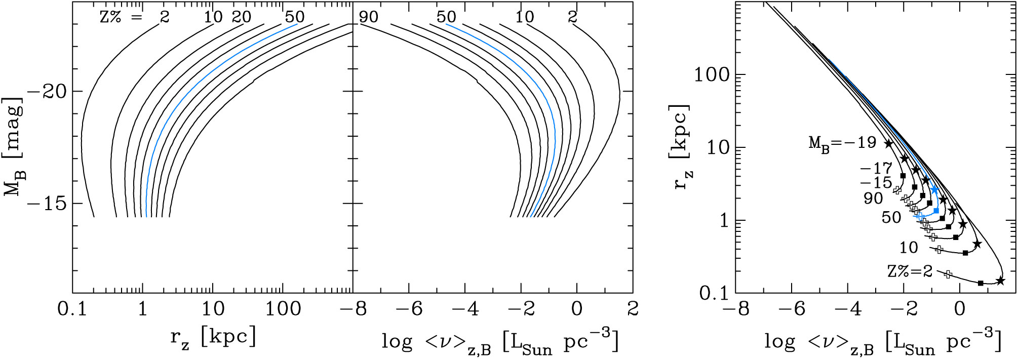
As with the projected effective parameters, the internal effective parameters display a similar behaviour of strongly curved relations, in which the midpoint of each curve depends on Z and therefore obviously does not reflect a separation based on physically different formation processes. The midpoint of the bend shifts from roughly -19 to -16 mag as Z changes from 2 to 90%. A value of $Z=50$
corresponds to the internal half-light radius
$Z=50$
corresponds to the internal half-light radius $r_{\rm e}$
and the mean luminosity density
$r_{\rm e}$
and the mean luminosity density $\langle \nu \rangle_{\rm e}$
, traced by the
$\langle \nu \rangle_{\rm e}$
, traced by the $Z=50$
curves in Figure 9. The similarity between the
$Z=50$
curves in Figure 9. The similarity between the $Z=50$
curve in the left-hand panel of Figure 9 and the
$Z=50$
curve in the left-hand panel of Figure 9 and the $Z=50$
curve in the left-hand panel of Figure 4 was expected, given that
$Z=50$
curve in the left-hand panel of Figure 4 was expected, given that $r_{\rm e} \approx 4/3 R_{\rm e}$
(Ciotti, Reference Ciotti1991). In addition, the similar patterns seen in both panels means that the different ratio of radii (
$r_{\rm e} \approx 4/3 R_{\rm e}$
(Ciotti, Reference Ciotti1991). In addition, the similar patterns seen in both panels means that the different ratio of radii ( $r_{z_1}/r_{z_2}$
) at fixed absolute magnitude, for different percentages
$r_{z_1}/r_{z_2}$
) at fixed absolute magnitude, for different percentages $z_1$
and
$z_1$
and $z_2$
, will result in
$z_2$
, will result in $\sigma^2 r/G$
mass estimates that depend on the percentage used to define r. As was seen in the middle panel of Figure 4, the ratio of radii again increasingly varies as the luminosity increases. This also coincides with an increased steepening of the velocity dispersion profile, impacting estimates of the dynamical mass (e.g. Wolf, 2011 Wolf et al., Reference Wolf, Martinez and Bullock2010; Forbes et al., Reference Forbes, Spitler and Graham2011, see their Section 9.2) and further undermining the use of
$\sigma^2 r/G$
mass estimates that depend on the percentage used to define r. As was seen in the middle panel of Figure 4, the ratio of radii again increasingly varies as the luminosity increases. This also coincides with an increased steepening of the velocity dispersion profile, impacting estimates of the dynamical mass (e.g. Wolf, 2011 Wolf et al., Reference Wolf, Martinez and Bullock2010; Forbes et al., Reference Forbes, Spitler and Graham2011, see their Section 9.2) and further undermining the use of $\sigma^2 r_{\rm e}/G$
in the brighter, non-dwarf, ETGs.
$\sigma^2 r_{\rm e}/G$
in the brighter, non-dwarf, ETGs.
The right-hand panel of Figure 9 reveals that one can expect a strong $\log r_{\rm e}$
–
$\log r_{\rm e}$
– $\log \langle \nu \rangle_{\rm e}$
relation for bright ETGs. This is because if one mis-measures the internal radius enclosing 50% of the light and obtains a radius containing say 20 or 80% of the total light, the associated mean luminosity density that one measures will largely shift one along the
$\log \langle \nu \rangle_{\rm e}$
relation for bright ETGs. This is because if one mis-measures the internal radius enclosing 50% of the light and obtains a radius containing say 20 or 80% of the total light, the associated mean luminosity density that one measures will largely shift one along the $\log r_{\rm e}$
–
$\log r_{\rm e}$
–
 $\log
\langle \nu \rangle_{\rm e}$
relation for bright ETGs (see also Trujillo et al., Reference Trujillo, Graham and Caon2001, their Section 4). At low luminosities, faint of the midpoint of the bend in these curved relations, the same such mis-measurement will move one away from the curved
$\log
\langle \nu \rangle_{\rm e}$
relation for bright ETGs (see also Trujillo et al., Reference Trujillo, Graham and Caon2001, their Section 4). At low luminosities, faint of the midpoint of the bend in these curved relations, the same such mis-measurement will move one away from the curved $\log r_{\rm e}$
–
$\log r_{\rm e}$
– $\log \langle \nu \rangle_{\rm e}$
relation. This behaviour can be seen in the
$\log \langle \nu \rangle_{\rm e}$
relation. This behaviour can be seen in the $\log r_{\rm e}$
–
$\log r_{\rm e}$
– $\log \nu_{\rm e}$
diagram of Graham et al., (Reference Graham, Merritt, Moore, Diemand and Terzić2006, see their Figure 2b).
$\log \nu_{\rm e}$
diagram of Graham et al., (Reference Graham, Merritt, Moore, Diemand and Terzić2006, see their Figure 2b).
The collective broadening that can be seen at faint absolute magnitudes in the right-hand panel of Figure 9 can be compared with the right-hand panel of Figure 5. Note that Figure 9 only shows data for light profiles with $n>1$
(
$n>1$
( $\mathfrak{M}_B \lt -14.3$
mag). Also bear in mind that the mean surface brightness (Figure 5) is 2.5 times the logarithm of the mean intensity, hence the greater range along the
$\mathfrak{M}_B \lt -14.3$
mag). Also bear in mind that the mean surface brightness (Figure 5) is 2.5 times the logarithm of the mean intensity, hence the greater range along the
 $\langle
\mu \rangle_{\rm e}$
axis in Figure 5 than compared to the
$\langle
\mu \rangle_{\rm e}$
axis in Figure 5 than compared to the
 $\log
\langle \nu \rangle_z$
axis in Figure 9.
$\log
\langle \nu \rangle_z$
axis in Figure 9.
5.2. Alternative internal radii
Similar to Subsection 4.2, we can explore the internal radii r where the internal density, $\nu$
, has dropped by a fixed amount from the value at some inner radius. Figure 8 reveals that, for Sérsic indices
$\nu$
, has dropped by a fixed amount from the value at some inner radius. Figure 8 reveals that, for Sérsic indices $n>0.5$
–1, the internal density profile rises steeply with decreasing radius. In the middle and right-hand panels of Figure 6, this rapid brightening of the projected surface brightness was circumvented by starting from the radius
$n>0.5$
–1, the internal density profile rises steeply with decreasing radius. In the middle and right-hand panels of Figure 6, this rapid brightening of the projected surface brightness was circumvented by starting from the radius $R=0.01$
and 0.1 kpc. Here, we start at
$R=0.01$
and 0.1 kpc. Here, we start at $r=0.01$
and 0.1 kpc to compute the internal radii where the internal luminosity density profile has dropped by a fixed amount from the density at these two inner radii. Figure 10 shows these alternative scale radii as a function of the absolute B-band magnitude (for magnitudes corresponding to
$r=0.01$
and 0.1 kpc to compute the internal radii where the internal luminosity density profile has dropped by a fixed amount from the density at these two inner radii. Figure 10 shows these alternative scale radii as a function of the absolute B-band magnitude (for magnitudes corresponding to $n>1$
). The relations seen there do not support an ETG divide at
$n>1$
). The relations seen there do not support an ETG divide at
 $\mathfrak{M}_B \approx
-18$
mag.
$\mathfrak{M}_B \approx
-18$
mag.
For each absolute magnitude, $\mathfrak{M}_B$
, one can see the internal radius where the logarithm of the luminosity density (
$\mathfrak{M}_B$
, one can see the internal radius where the logarithm of the luminosity density ( $\nu$
, in units of
$\nu$
, in units of $L_{\odot,B}$
pc-3) has decreased by a fixed amount from its value at
$L_{\odot,B}$
pc-3) has decreased by a fixed amount from its value at $r=0.01$
kpc (left panel) and
$r=0.01$
kpc (left panel) and $r=0.1$
kpc (right panel).
$r=0.1$
kpc (right panel).
5.3. Isodensity radii
Isodensity radii define a two-dimensional surface, such as a sphere, within a three-dimensional space. These radii are the internal analog to the projected isophotal radii seen in Subsection 4.3 and are naturally considered a better measure to define the radii of three-dimensional stellar systems. This is simply because isophotes can display an artificial (not physical) contour, arising from the projected column density through a galaxy, rather than a real boundary of equal density.
Figure 11 displays the $\mathfrak{M}_B$
–
$\mathfrak{M}_B$
– $R_{\rm isodensity}$
relations for five different luminosity densities. The trends reveal no evidence for a divide at
$R_{\rm isodensity}$
relations for five different luminosity densities. The trends reveal no evidence for a divide at $\mathfrak{M}_B \approx -18$
mag.
$\mathfrak{M}_B \approx -18$
mag.
For each absolute magnitude, $\mathfrak{M}_B$
, one can see the internal radius where the logarithm of the luminosity density (
$\mathfrak{M}_B$
, one can see the internal radius where the logarithm of the luminosity density ( $\nu$
, in units of
$\nu$
, in units of $L_{\odot,B}$
pc-3) equals one of the five different values.
$L_{\odot,B}$
pc-3) equals one of the five different values.
While this concludes the recapitulation of the previous section but performed using internal parameters, it would be somewhat incomplete to proceed without having used the virial radii which are popular among theorists. Therefore, the following subsection presents this, along with an observer-inspired variation.
5.4. Virial radii
The integrated luminosity, within spheres centred on a galaxy, is given by
 \begin{equation}
L_{n}(s)=I_{\rm e}{\rm e}^{b}R_{\rm e}^{2}\, 4\pi \int _{0}^{s}\nu _{n}(s')s'^{2}ds',
\label{eqn28}
\end{equation}
\begin{equation}
L_{n}(s)=I_{\rm e}{\rm e}^{b}R_{\rm e}^{2}\, 4\pi \int _{0}^{s}\nu _{n}(s')s'^{2}ds',
\label{eqn28}
\end{equation}
and is shown in Figure 12 for our representative set of profiles from Figure 8.
Representative, cumulative luminosity profiles for different Sérsic indices n, as matched to the light profiles shown in Figure 2.
Multiplying by a stellar mass-to-light ratio gives the cumulative stellar mass profiles. The luminosity density profiles $\nu(r)$
(equation (27)) were converted into stellar mass density profiles
$\nu(r)$
(equation (27)) were converted into stellar mass density profiles $\rho(r)$
, using a constant B-band stellar mass-to-light ratio of
$\rho(r)$
, using a constant B-band stellar mass-to-light ratio of $M/L_B=8$
.
$M/L_B=8$
.
Following Macciò, Murante, & Bonometto (Reference Macciò, Murante and Bonometto2003, their equation 1.1; see also Bryan & Norman, Reference Bryan and Norman1998), a proxyFootnote r is used for the virial radius defined as the radius of the sphere within which the average (stellar mass) density is equal to
 $18\, \Pi^2\, \Omega_{\rm matter}^{0.45}\, \rho_{\rm critical}
\approx 177.7 \times 0.589 \times \rho_{\rm critical}
\approx 104.6\, \rho_{\rm critical}
\approx (339.5\,\, \Omega_{\rm matter})\, \rho_{\rm critical}$
. The Planck 2015 results (Planck et al., 2016) give
$18\, \Pi^2\, \Omega_{\rm matter}^{0.45}\, \rho_{\rm critical}
\approx 177.7 \times 0.589 \times \rho_{\rm critical}
\approx 104.6\, \rho_{\rm critical}
\approx (339.5\,\, \Omega_{\rm matter})\, \rho_{\rm critical}$
. The Planck 2015 results (Planck et al., 2016) give $\Omega_{\rm matter}=0.308\pm0.012$
and thus
$\Omega_{\rm matter}=0.308\pm0.012$
and thus
 $339.5\, \Omega_{\rm matter} =
104.6$
. They also report
$339.5\, \Omega_{\rm matter} =
104.6$
. They also report $H_0 = 67.8\pm0.9$
km s-1 Mpc-1 and thus
$H_0 = 67.8\pm0.9$
km s-1 Mpc-1 and thus $\rho_{\rm critical} \equiv 3H^2_0/(8\Pi G) = 0.864\times10^{-26}$
kg m-3, or
$\rho_{\rm critical} \equiv 3H^2_0/(8\Pi G) = 0.864\times10^{-26}$
kg m-3, or $39.3\, {\rm M}_{\odot}\, {\rm kpc}^{-3}$
. The popular, and smaller,
$39.3\, {\rm M}_{\odot}\, {\rm kpc}^{-3}$
. The popular, and smaller, $r_{200}$
radius (Carlberg, Yee, & Ellingson, Reference Carlberg, Yee and Ellingson1997), within which the average (stellar mass) density is equal to
$r_{200}$
radius (Carlberg, Yee, & Ellingson, Reference Carlberg, Yee and Ellingson1997), within which the average (stellar mass) density is equal to $200 \rho_{\rm critical}$
, is additionally calculated. The virial radius and the
$200 \rho_{\rm critical}$
, is additionally calculated. The virial radius and the $r_{200}$
radius (associated with the stellar mass and thus ignoring any potential dark matter halo) is shown in Figure 13 as a function of the absolute magnitudeFootnote s.
$r_{200}$
radius (associated with the stellar mass and thus ignoring any potential dark matter halo) is shown in Figure 13 as a function of the absolute magnitudeFootnote s.
The virial radius is shown as a function of the B-band absolute magnitude $\mathfrak{M}_B$
. The average stellar mass density within the virial radius equals
$\mathfrak{M}_B$
. The average stellar mass density within the virial radius equals $104.5\, \rho_{\rm critical}$
. Also shown is the radius
$104.5\, \rho_{\rm critical}$
. Also shown is the radius $r_{200}$
within which the average density equals
$r_{200}$
within which the average density equals $(200/\Omega_{\rm matter}) \rho_{\rm critical}$
. The slope equals -3, except for the luminous galaxies with high Sérsic indices, and thus long tails to their light profiles, with stars beyond the virial radius.
$(200/\Omega_{\rm matter}) \rho_{\rm critical}$
. The slope equals -3, except for the luminous galaxies with high Sérsic indices, and thus long tails to their light profiles, with stars beyond the virial radius.
For $\mathfrak{M}_B \mathbin{\lower.3ex\hbox{$\buildrel\gt\over
{\smash{\scriptstyle\sim}\vphantom{_x}}$}} -22$
mag, the slope of the
$\mathfrak{M}_B \mathbin{\lower.3ex\hbox{$\buildrel\gt\over
{\smash{\scriptstyle\sim}\vphantom{_x}}$}} -22$
mag, the slope of the $\mathfrak{M}_B$
–
$\mathfrak{M}_B$
– $r_{\rm virial}$
and
$r_{\rm virial}$
and $\mathfrak{M}_B$
–
$\mathfrak{M}_B$
– $r_{200}$
relation is 7.5. Converting the magnitude axis to
$r_{200}$
relation is 7.5. Converting the magnitude axis to $\log({\rm luminosity})$
and applying a constant stellar mass-to-light ratio (as was assumed for calculating the virial radii) would give a slope of
$\log({\rm luminosity})$
and applying a constant stellar mass-to-light ratio (as was assumed for calculating the virial radii) would give a slope of $7.5/2.5=3$
for the logarithmic mass–size relation. Thus, for
$7.5/2.5=3$
for the logarithmic mass–size relation. Thus, for $\mathfrak{M}_B \mathbin{\lower.3ex\hbox{$\buildrel\gt\over
{\smash{\scriptstyle\sim}\vphantom{_x}}$}} -22$
mag, the radii are large enough that they enclose the bulk of the stellar mass M, and thus, the pursuit of a constant, average enclosed density (mass/volume) is simply giving radii that meet the condition
$\mathfrak{M}_B \mathbin{\lower.3ex\hbox{$\buildrel\gt\over
{\smash{\scriptstyle\sim}\vphantom{_x}}$}} -22$
mag, the radii are large enough that they enclose the bulk of the stellar mass M, and thus, the pursuit of a constant, average enclosed density (mass/volume) is simply giving radii that meet the condition $M \propto r^3$
. As such, the masses may as well be point masses, as the information in the density profile is effectively lost.
$M \propto r^3$
. As such, the masses may as well be point masses, as the information in the density profile is effectively lost.
5.4.1. A variation
Here, a new internal galaxy radius, $r_{\rm g}$
, is introduced. It is such that the average density within this radius equals some fraction of the local density at that radius. Mathematically, this can be thought of as a variation of the virial radius, which can be expressed as
$r_{\rm g}$
, is introduced. It is such that the average density within this radius equals some fraction of the local density at that radius. Mathematically, this can be thought of as a variation of the virial radius, which can be expressed as
 \begin{equation}
\log (104.6)=\log \langle \rho \rangle_{r_{\rm virial}} - \log \rho_{\rm critical}.
\label{eqn29}
\end{equation}
\begin{equation}
\log (104.6)=\log \langle \rho \rangle_{r_{\rm virial}} - \log \rho_{\rm critical}.
\label{eqn29}
\end{equation}
The variation introduced here can be written as
 \begin{equation}
\log ( \mathrm{H} )=\log \langle \rho \rangle_{r_{\rm g}} - \log \rho(r=r_{\rm g}).
\label{eqn30}
\end{equation}
\begin{equation}
\log ( \mathrm{H} )=\log \langle \rho \rangle_{r_{\rm g}} - \log \rho(r=r_{\rm g}).
\label{eqn30}
\end{equation}
This radius is somewhat akin to Petrosian (Reference Petrosian1976) radii, used by observers, which is such that the average intensity within some projected radius $R_{\rm P}$
divided by the intensity at that radius (denoted
$R_{\rm P}$
divided by the intensity at that radius (denoted $\eta$
) equals some constant value, typically 5 (e.g. Bershady, Jangren, & Conselice Reference Bershady, Jangren and Conselice2000; Blanton et al., Reference Blanton, Dalcanton and Eisenstein2001). For Petrosian radii, one has the expression
$\eta$
) equals some constant value, typically 5 (e.g. Bershady, Jangren, & Conselice Reference Bershady, Jangren and Conselice2000; Blanton et al., Reference Blanton, Dalcanton and Eisenstein2001). For Petrosian radii, one has the expression
 \begin{equation}
-2.5 \log [\eta=5]=\langle\mu\rangle_{R_{\rm P}} - \mu(R=R_{\rm P})
\label{eqn31}
\end{equation}
\begin{equation}
-2.5 \log [\eta=5]=\langle\mu\rangle_{R_{\rm P}} - \mu(R=R_{\rm P})
\label{eqn31}
\end{equation}
Figure 14 presents these new galaxy radii (equation (30)) for values of $\log \mathrm{H} =$
0.5, 0.6, 0.8, and 1.0. One can see that they, unlike the virial radii, are no longer too large to be unaffected by the galaxies’ structure. They behave in a fashion somewhat similar to the internal radii containing different fractions of the galaxy light. Once again, no convincing evidence for a dichotomy at a fixed magnitude is apparent.
$\log \mathrm{H} =$
0.5, 0.6, 0.8, and 1.0. One can see that they, unlike the virial radii, are no longer too large to be unaffected by the galaxies’ structure. They behave in a fashion somewhat similar to the internal radii containing different fractions of the galaxy light. Once again, no convincing evidence for a dichotomy at a fixed magnitude is apparent.
Internal radius where the mean enclosed density equals some fraction of the density at that radius.
6. Case studies
Graham & Guzmán (Reference Graham and Guzmán2003) compiled data for $\sim$
250 ETGs to demonstrate the unified nature of dwarf and ordinary ETGs across the alleged divide at
$\sim$
250 ETGs to demonstrate the unified nature of dwarf and ordinary ETGs across the alleged divide at $\mathfrak{M} \approx -18$
mag. This data set included Hubble Space Telescope (HST)-resolved dwarf ETGs plus HST-resolved, ordinary, ETGs from Faber et al. (Reference Faber, Tremaine and Ajhar1997), among which those ETGs without depleted cores followed the
$\mathfrak{M} \approx -18$
mag. This data set included Hubble Space Telescope (HST)-resolved dwarf ETGs plus HST-resolved, ordinary, ETGs from Faber et al. (Reference Faber, Tremaine and Ajhar1997), among which those ETGs without depleted cores followed the $\mathfrak{M}$
–
$\mathfrak{M}$
– $\mu_0$
relation (equation (17)). Since then, a few additional ETG data sets have come forth, and it is insightful to elaborate on alleged discrepancies or differences using two of these.
$\mu_0$
relation (equation (17)). Since then, a few additional ETG data sets have come forth, and it is insightful to elaborate on alleged discrepancies or differences using two of these.
6.1. Case study 1: Ferrarese et al. (Reference Ferrarese, Côté and Jordán2006)
Ferrarese et al. (Reference Ferrarese, Côté and Jordán2006) imaged 100 Virgo cluster ETGs with HST and the F475W filter (transformed to the AB photometric system’s g-band) as a part of the ‘Advanced Camera for Surveys Virgo Cluster Survey’ (ACSVCS; Côté et al., Reference Côté, Blakeslee and Ferrarese2004; Ferrarese et al., Reference Ferrarese, Côté and Jordán2006). Ferrarese et al. (Reference Ferrarese, Côté and Jordán2006) fit seeing-convolved Sérsic and core-Sérsic models (plus optional nuclear excesses) to the (geometric mean)-axisFootnote t surface brightness profiles. As such, because they take the ellipticity profile into account, their models can be readily integrated to obtain the total galaxy magnitude. The (surface brightness fluctuation)-based distances from Mei et al. (Reference Mei, Blakeslee and Côté2007) have been used to convert these model magnitudes into absolute magnitudes, and they have been corrected for Galactic extinction using the values from Schlafly & Finkbeiner (Reference Schlafly and Finkbeiner2011), as tabulated in the NASA/IPAC Extragalactic Database (NED)Footnote u.
Of these 100 galaxies, 2 (VCC 1535; VCC 1030) could not be modelled by Ferrarese et al. (Reference Ferrarese, Côté and Jordán2006) due to dust, and 2 (VCC 1250 and VCC 1512) have core-Sérsic fits which Ferrarese et al. (Reference Ferrarese, Côté and Jordán2006, see their Section 4.2) discredit — and rightfully so given that the $R_{\rm e}$
values hit their limit of 490 arcsec, as was also the case for VCC 575 (
$R_{\rm e}$
values hit their limit of 490 arcsec, as was also the case for VCC 575 ( $\mathfrak{M}_B = -17.61$
mag). In addition to these five galaxies, the S0 galaxy VCC 1321 (NGC 4489,
$\mathfrak{M}_B = -17.61$
mag). In addition to these five galaxies, the S0 galaxy VCC 1321 (NGC 4489, $\mathfrak{M}_B = -18.20$
mag) which was reported to have an unusually high galaxy Sérsic index of
$\mathfrak{M}_B = -18.20$
mag) which was reported to have an unusually high galaxy Sérsic index of $\sim$
6 (cf.
$\sim$
6 (cf. $2.3\pm0.5$
from Table C1 of Krajnović et al., 2013) is also excluded.
$2.3\pm0.5$
from Table C1 of Krajnović et al., 2013) is also excluded.
Here, we will see how the linear $\mathfrak{M}$
–
$\mathfrak{M}$
– $\mu_0$
and
$\mu_0$
and $\mathfrak{M}$
–n relationsFootnote v, spanning the Virgo ETG sample’s full magnitude range, explain the curved trends in diagrams involving effective radii and effective surface brightnesses. The following two g-band equations approximate the distribution of data seen in the upper panels of Figure 15:
$\mathfrak{M}$
–n relationsFootnote v, spanning the Virgo ETG sample’s full magnitude range, explain the curved trends in diagrams involving effective radii and effective surface brightnesses. The following two g-band equations approximate the distribution of data seen in the upper panels of Figure 15:
Sample of 94 Virgo cluster ETGs from Ferrarese et al. (Reference Ferrarese, Côté and Jordán2006). Top row: The Sérsic parameters, including $\mathfrak{M}_g$
and
$\mathfrak{M}_g$
and $\mu_{0,g}$
, are from fits to the (geometric mean)-axis light profiles. The lines are defined in equations 32 and 33. Middle and bottom rows: The solid curves are predictions based on the linear fits in the top panels. The three equal-dashed curves in the lower panels show the
$\mu_{0,g}$
, are from fits to the (geometric mean)-axis light profiles. The lines are defined in equations 32 and 33. Middle and bottom rows: The solid curves are predictions based on the linear fits in the top panels. The three equal-dashed curves in the lower panels show the $\mathfrak{M}_g = -15$
mag boundary. Looking at the two lower left-hand panels, one might be inclined to call for a divide at
$\mathfrak{M}_g = -15$
mag boundary. Looking at the two lower left-hand panels, one might be inclined to call for a divide at $\mathfrak{M} = -20.5\pm0.5$
mag, while looking at the two lower right-hand panels, one may instead be inclined to advocate for a divide at
$\mathfrak{M} = -20.5\pm0.5$
mag, while looking at the two lower right-hand panels, one may instead be inclined to advocate for a divide at
 $\mathfrak{M} =
-18\pm1$
mag.
$\mathfrak{M} =
-18\pm1$
mag.
 \begin{eqnarray}
\mathfrak{M}_g &=& -10.5\log(n) - 14.0, {\rm and} \label{eqn32}\end{eqnarray}
\begin{eqnarray}
\mathfrak{M}_g &=& -10.5\log(n) - 14.0, {\rm and} \label{eqn32}\end{eqnarray}
 \begin{eqnarray}
\mathfrak{M}_g &=& 0.63\mu_{0,g} -28.4,
\label{eqn33}\end{eqnarray}
\begin{eqnarray}
\mathfrak{M}_g &=& 0.63\mu_{0,g} -28.4,
\label{eqn33}\end{eqnarray}
The predicted g-band $\mathfrak{M}$
–
$\mathfrak{M}$
– $\mu_z$
and
$\mu_z$
and $\mathfrak{M}$
–
$\mathfrak{M}$
– $R_z$
distributions are presented in the middle and lower panels of Figure 15 for
$R_z$
distributions are presented in the middle and lower panels of Figure 15 for $z=0.05, 0.5,$
and
$z=0.05, 0.5,$
and $0.95$
. Similar results are obtained with the
$0.95$
. Similar results are obtained with the $\mathfrak{M}$
–
$\mathfrak{M}$
– $\langle \mu \rangle$
diagram and also when using their data obtained through the F850LP filter.
$\langle \mu \rangle$
diagram and also when using their data obtained through the F850LP filter.
The middle and lower panels of Figure 15 should be compared with Figure 117 in Ferrarese et al. (Reference Ferrarese, Côté and Jordán2006), which used quantities at $z=0.05$
and 0.5 (
$z=0.05$
and 0.5 ( $Z=5$
% and 50%), and compared with Figure 76 in K09 which used quantities at 50%. The series of linear equations 17– 26 in Ferrarese et al. (Reference Ferrarese, Côté and Jordán2006) — used to approximate the bright and faint ends of their
$Z=5$
% and 50%), and compared with Figure 76 in K09 which used quantities at 50%. The series of linear equations 17– 26 in Ferrarese et al. (Reference Ferrarese, Côté and Jordán2006) — used to approximate the bright and faint ends of their $\mathfrak{M}$
–
$\mathfrak{M}$
– $\mu_{\rm e}$
,
$\mu_{\rm e}$
, $\mathfrak{M}$
–
$\mathfrak{M}$
– $R_{\rm e}$
,
$R_{\rm e}$
, $\mathfrak{M}$
–
$\mathfrak{M}$
– $\mu_5,$
and
$\mu_5,$
and $\mathfrak{M}$
–
$\mathfrak{M}$
– $R_5$
distributions — does not adequately capture the curved nature of the scaling relations which unify the faint and bright ETGs in these diagrams. Their equations have been fit separately to the core-Sérsic and Sérsic galaxies, implying a division between these two galaxy types in these diagrams. However, their set of linear approximations are not only dependent upon the magnitude range included in the fit, but they go against the premise of a continuity in these diagrams and against the understanding that the different slopes at bright and faint magnitudes cannot be used to interpret signs of different galaxy types or formation physics in diagrams involving ‘effective’ parameters. Ferrarese et al. (Reference Ferrarese, Côté and Jordán2006) understood that there is a continuity at
$R_5$
distributions — does not adequately capture the curved nature of the scaling relations which unify the faint and bright ETGs in these diagrams. Their equations have been fit separately to the core-Sérsic and Sérsic galaxies, implying a division between these two galaxy types in these diagrams. However, their set of linear approximations are not only dependent upon the magnitude range included in the fit, but they go against the premise of a continuity in these diagrams and against the understanding that the different slopes at bright and faint magnitudes cannot be used to interpret signs of different galaxy types or formation physics in diagrams involving ‘effective’ parameters. Ferrarese et al. (Reference Ferrarese, Côté and Jordán2006) understood that there is a continuity at
 $\mathfrak{M} =
-18$
mag and a divide at
$\mathfrak{M} =
-18$
mag and a divide at $\mathfrak{M} \approx -20.5$
mag — as did Gavazzi et al. (Reference Gavazzi, Donati and Cucciati2005); Côté et al., Reference Côté, Ferrarese and Jordán2007, Reference Côté, Piatek and Ferrarese2006; Misgeld, Mieske, & Hilker, Reference Misgeld, Mieske and Hilker2008 2009; and Chen et al., Reference Chen, Côté, West, Peng and Ferrarese2010 — but diagrams involving effective radii and effective surface brightnesses can not be used to make this diagnosis. Similarly, the colour-coding used by K09 (see their Figure 76) is inappropriate and misleading.
$\mathfrak{M} \approx -20.5$
mag — as did Gavazzi et al. (Reference Gavazzi, Donati and Cucciati2005); Côté et al., Reference Côté, Ferrarese and Jordán2007, Reference Côté, Piatek and Ferrarese2006; Misgeld, Mieske, & Hilker, Reference Misgeld, Mieske and Hilker2008 2009; and Chen et al., Reference Chen, Côté, West, Peng and Ferrarese2010 — but diagrams involving effective radii and effective surface brightnesses can not be used to make this diagnosis. Similarly, the colour-coding used by K09 (see their Figure 76) is inappropriate and misleading.
6.2. Case study 2: Kormendy et al. (Reference Kormendy, Fisher, Cornell and Bender2009)
K09 acceptFootnote w the $\mathfrak{M}$
–n relation (see their Figure 33) but they deny the existence of a linear
$\mathfrak{M}$
–n relation (see their Figure 33) but they deny the existence of a linear $\mathfrak{M}$
–
$\mathfrak{M}$
– $\mu_0$
relation unifying dwarf and ordinary ETGs (see their Figure 1). This follows on from Kormendy (Reference Kormendy1985, see his Figure 3), which produced an
$\mu_0$
relation unifying dwarf and ordinary ETGs (see their Figure 1). This follows on from Kormendy (Reference Kormendy1985, see his Figure 3), which produced an $\mathfrak{M}_B$
–
$\mathfrak{M}_B$
– $\mu_0$
diagram with a sample selection that had an absence of ETGs with magnitudes
$\mu_0$
diagram with a sample selection that had an absence of ETGs with magnitudes $-17 \mathbin{\lower.3ex\hbox{$\buildrel\gt\over
{\smash{\scriptstyle\sim}\vphantom{_x}}$}} \mathfrak{M}_B \mathbin{\lower.3ex\hbox{$\buildrel\gt\over
{\smash{\scriptstyle\sim}\vphantom{_x}}$}} -20.5$
mag (
$-17 \mathbin{\lower.3ex\hbox{$\buildrel\gt\over
{\smash{\scriptstyle\sim}\vphantom{_x}}$}} \mathfrak{M}_B \mathbin{\lower.3ex\hbox{$\buildrel\gt\over
{\smash{\scriptstyle\sim}\vphantom{_x}}$}} -20.5$
mag ( $H_0=50$
km s-1 Mpc-1), making it difficult to know where a transition may occur.Footnote x Further complicating the situation was that the faint ETG data in Kormendy (Reference Kormendy1985) did not produce the known
$H_0=50$
km s-1 Mpc-1), making it difficult to know where a transition may occur.Footnote x Further complicating the situation was that the faint ETG data in Kormendy (Reference Kormendy1985) did not produce the known $\mathfrak{M}_B$
–
$\mathfrak{M}_B$
– $\mu_{0,B}$
trend (e.g. Binggeli et al. Reference Binggeli, Sandage and Tarenghi1984, see their Figure 8)Footnote y whose distribution points towards the faint-end of the
$\mu_{0,B}$
trend (e.g. Binggeli et al. Reference Binggeli, Sandage and Tarenghi1984, see their Figure 8)Footnote y whose distribution points towards the faint-end of the $\mathfrak{M}_B$
–
$\mathfrak{M}_B$
– $\mu_{0,B}$
sequence for bright ETGs with depleted cores. That is, according to the data in Kormendy (Reference Kormendy1985), the ETGs fainter than
$\mu_{0,B}$
sequence for bright ETGs with depleted cores. That is, according to the data in Kormendy (Reference Kormendy1985), the ETGs fainter than $\mathfrak{M}_B \approx -17$
mag follow a distribution with a steeper slope in the
$\mathfrak{M}_B \approx -17$
mag follow a distribution with a steeper slope in the $\mathfrak{M}_B$
–
$\mathfrak{M}_B$
– $\mu_{0,B}$
diagram than shown in the right-hand panel of Figure 1, such that the distribution of faint ETGs in Kormendy (Reference Kormendy1985) points to the bright-end of the distribution of ETGs with depleted cores. Despite the ongoing rejection by K09 for a unifying
$\mu_{0,B}$
diagram than shown in the right-hand panel of Figure 1, such that the distribution of faint ETGs in Kormendy (Reference Kormendy1985) points to the bright-end of the distribution of ETGs with depleted cores. Despite the ongoing rejection by K09 for a unifying $\mathfrak{M}$
–
$\mathfrak{M}$
– $\mu_0$
relation across
$\mu_0$
relation across $\mathfrak{M}_B = -18$
mag (
$\mathfrak{M}_B = -18$
mag ( $\mathfrak{M}_{V_T} \approx -19$
mag), K09 did not actually show the
$\mathfrak{M}_{V_T} \approx -19$
mag), K09 did not actually show the $\mathfrak{M}$
–
$\mathfrak{M}$
– $\mu_0$
diagram for their data set nor the
$\mu_0$
diagram for their data set nor the $\mathfrak{M}$
–
$\mathfrak{M}$
– $\mu_5$
diagram used by Ferrarese et al. (Reference Ferrarese, Côté and Jordán2006).
$\mu_5$
diagram used by Ferrarese et al. (Reference Ferrarese, Côté and Jordán2006).
K09 also excluded many of the ETGs in Ferrarese et al. (Reference Ferrarese, Côté and Jordán2006) because they wanted to work with what they thought was a sample of predominantly one-component galaxies, that is, no lenticular galaxies. K09 effectively thinned-out much of the population of ETGs from $-18 > \mathfrak{M}_B > -20.5$
mag. This resulted in a sample of 42 ETGs, including 10 dwarf ETGs. However, 5 of the 32 non-dwarf galaxies were subsequently identified as S0 galaxies by K09. Furthermore, another 5 were rare compact elliptical (cE) galaxies, taken from Table XIII of Binggeli et al. (Reference Binggeli, Kunth, Thuan and Van1985; who note in Part 3 of their Appendix that the M32-like galaxies are vastly outnumbered by dwarf ETGs of similar magnitude:
$-18 > \mathfrak{M}_B > -20.5$
mag. This resulted in a sample of 42 ETGs, including 10 dwarf ETGs. However, 5 of the 32 non-dwarf galaxies were subsequently identified as S0 galaxies by K09. Furthermore, another 5 were rare compact elliptical (cE) galaxies, taken from Table XIII of Binggeli et al. (Reference Binggeli, Kunth, Thuan and Van1985; who note in Part 3 of their Appendix that the M32-like galaxies are vastly outnumbered by dwarf ETGs of similar magnitude: $-14 > \mathfrak{M}_B > -18$
mag). The cE galaxies are thought to be heavily stripped disc galaxies (e.g. Rood, Reference Rood1965; Bekki et al., Reference Bekki, Couch, Drinkwater and Gregg2001; Graham, Reference Graham2002b; Chilingarian et al., Reference Chilingarian, Cayatte and Revaz2009), while the isolated cE galaxies may have either never acquired a significant disc or may have been ejected from a cluster after losing much of their disc (e.g. Chilingarian & Zolotukhin, Reference Chilingarian and Zolotukhin2015). The cE galaxies are two-component systems, likely dominated by a remnant bulge, and are known to overlap with the bulges of spiral and S0 galaxies in the scaling diagrams (e.g. Graham Reference Graham, Oswalt and Keel2013, see his Figure 1). This over-representation of cE galaxies, relative to normal galaxies, in K09 is inappropriate for two reasons. In terms of a sample providing a balanced representation of galaxies, there should be
$-14 > \mathfrak{M}_B > -18$
mag). The cE galaxies are thought to be heavily stripped disc galaxies (e.g. Rood, Reference Rood1965; Bekki et al., Reference Bekki, Couch, Drinkwater and Gregg2001; Graham, Reference Graham2002b; Chilingarian et al., Reference Chilingarian, Cayatte and Revaz2009), while the isolated cE galaxies may have either never acquired a significant disc or may have been ejected from a cluster after losing much of their disc (e.g. Chilingarian & Zolotukhin, Reference Chilingarian and Zolotukhin2015). The cE galaxies are two-component systems, likely dominated by a remnant bulge, and are known to overlap with the bulges of spiral and S0 galaxies in the scaling diagrams (e.g. Graham Reference Graham, Oswalt and Keel2013, see his Figure 1). This over-representation of cE galaxies, relative to normal galaxies, in K09 is inappropriate for two reasons. In terms of a sample providing a balanced representation of galaxies, there should be $\sim$
200 times (I. Chilingarian 2018, priv. comm.) fewer cE galaxies than non-cE galaxies across their co-existing range in absolute magnitude. Second, the cE galaxies are more akin to bulges, and as such, they are better compared with bulges than with parameters from single Sérsic fits to ETGs that typically contain bulges and discs.
$\sim$
200 times (I. Chilingarian 2018, priv. comm.) fewer cE galaxies than non-cE galaxies across their co-existing range in absolute magnitude. Second, the cE galaxies are more akin to bulges, and as such, they are better compared with bulges than with parameters from single Sérsic fits to ETGs that typically contain bulges and discs.
As for the five galaxies identified by K09 as lenticular galaxies, K09 performed a bulge/disc decomposition for these. As with their fitting of a single Sérsic model, they did not convolve their models with the central image’s point spread function but excluded by eye the region they considered to be affected by either nuclear excesses or a partially depleted core. They then used the bulge parameters rather than the galaxy parameters for these 5 galaxies to compare with the galaxy parameters of the remaining galaxies which they thought were pressure-supported, single-component systems (with additional small nuclear excesses or cores). However, Emsellem et al. (Reference Emsellem, Cappellari and Krajnović2011, see their Table B1) report on the internal kinematics for the brightest 19 of the supposed 27 ( $=32-5$
) ‘elliptical’ galaxies in K09. They reveal that 10 of these 19 are ‘fast rotators’, and Krajnović et al. (2013) provide bulge/disc decompositions for 7 of them. Furthermore, Toloba et al. (Reference Toloba, Guhathakurta and Boselli2015) contains internal kinematical information for 6 of the 10 ‘dwarf spheroidal’ galaxies in K09, reporting that 4 of these 6 are ‘fast rotators’. K09 have therefore plotted a mixture of bulge parameters (for 5 S0 galaxies) and galaxy parameters (for at least 11, and likely more, S0 galaxies). This blurs prospects for identifying connections in parameter scaling diagrams, and it explains why K09 did not find the known
$=32-5$
) ‘elliptical’ galaxies in K09. They reveal that 10 of these 19 are ‘fast rotators’, and Krajnović et al. (2013) provide bulge/disc decompositions for 7 of them. Furthermore, Toloba et al. (Reference Toloba, Guhathakurta and Boselli2015) contains internal kinematical information for 6 of the 10 ‘dwarf spheroidal’ galaxies in K09, reporting that 4 of these 6 are ‘fast rotators’. K09 have therefore plotted a mixture of bulge parameters (for 5 S0 galaxies) and galaxy parameters (for at least 11, and likely more, S0 galaxies). This blurs prospects for identifying connections in parameter scaling diagrams, and it explains why K09 did not find the known $\mathfrak{M}$
–n or
$\mathfrak{M}$
–n or $\mathfrak{M}$
–
$\mathfrak{M}$
– $\mu_0$
relations. Given that bulges and ETGs follow a different size–luminosity relation, they cannot follow the same
$\mu_0$
relations. Given that bulges and ETGs follow a different size–luminosity relation, they cannot follow the same $\mathfrak{M}$
–n and
$\mathfrak{M}$
–n and $\mathfrak{M}$
–
$\mathfrak{M}$
– $\mu_0$
relations (see 4.1). The
$\mu_0$
relations (see 4.1). The $\mathfrak{M}$
–n diagram in K09 is thus a blurring of two distributions, which have been separated here in Figure 16.
$\mathfrak{M}$
–n diagram in K09 is thus a blurring of two distributions, which have been separated here in Figure 16.
Sample of 42 stellar systems in the Virgo cluster from K09, comprising ordinary ETGs (large red circles), 5 bulges of ETGs (light blue squares, NGC: 4570, 4660, 4564, 4489, 4318), and 6 compact elliptical galaxies (dark blue stars, VCC: 1297, 1192, 1440, 1627, 1199, 1545) which are considered to be the remnant bulges of stripped disc galaxies. An additional 128 Virgo cluster ‘dwarf’ ETGs from Binggeli & Jerjen (Reference Binggeli and Jerjen1998) show the extension to fainter magnitudes. A rough $B-V=0.8$
colour was applied uniformly to this latter sample of B-band data. Top panel: The parameters are from Table 1 in K09, where the absolute magnitudes
$B-V=0.8$
colour was applied uniformly to this latter sample of B-band data. Top panel: The parameters are from Table 1 in K09, where the absolute magnitudes $\mathfrak{M}_{V_T}$
were derived independently of the Sérsic model for the ETGs and cE galaxies and are from their column 11; the Sérsic indices are major-axis values; and the central surface brightnesses are the
$\mathfrak{M}_{V_T}$
were derived independently of the Sérsic model for the ETGs and cE galaxies and are from their column 11; the Sérsic indices are major-axis values; and the central surface brightnesses are the $R=0$
values from their Sérsic models fit either to the galaxy or, in 5 instances, the bulge component. Expressions for the red ETG lines are provided in equations 34 and 35. Middle and lower rows: Similar to Figure 15. The three equal dashed curves show the
$R=0$
values from their Sérsic models fit either to the galaxy or, in 5 instances, the bulge component. Expressions for the red ETG lines are provided in equations 34 and 35. Middle and lower rows: Similar to Figure 15. The three equal dashed curves show the $\mathfrak{M}_{V_T} = -14$
mag boundary. Neither the absolute magnitudes, effective half-light (50%) radii, nor effective surface brightnesses in the lower middle panels are from the Sérsic model but were instead obtained independently from 2D profile integration by K09. The 10% and 95% radii and surface brightnesses were derived from the Sérsic model.
$\mathfrak{M}_{V_T} = -14$
mag boundary. Neither the absolute magnitudes, effective half-light (50%) radii, nor effective surface brightnesses in the lower middle panels are from the Sérsic model but were instead obtained independently from 2D profile integration by K09. The 10% and 95% radii and surface brightnesses were derived from the Sérsic model.
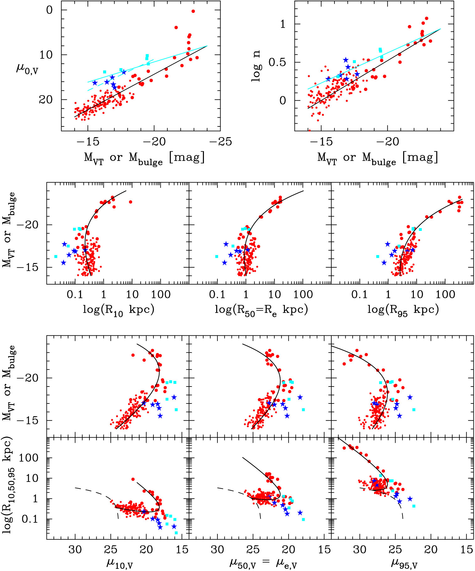
The upper panels in Figure 16 display the $\mathfrak{M}$
–
$\mathfrak{M}$
– $\mu_0$
(Vega V-band mag) diagram using the data from K09. One can see that there is an
$\mu_0$
(Vega V-band mag) diagram using the data from K09. One can see that there is an $\mathfrak{M}$
–
$\mathfrak{M}$
– $\mu_0$
relation for ETGs, although a couple of high
$\mu_0$
relation for ETGs, although a couple of high $-n$
ETGs appear to have had their Sérsic index over-estimated and their total magnitudes under-estimatedFootnote z by the (roughly) isophotal magnitudes advocated by K09 and used here for comparative purposes. The following equations represent the lines for ETG shown in the upper row of Figure 16.
$-n$
ETGs appear to have had their Sérsic index over-estimated and their total magnitudes under-estimatedFootnote z by the (roughly) isophotal magnitudes advocated by K09 and used here for comparative purposes. The following equations represent the lines for ETG shown in the upper row of Figure 16.
 \begin{eqnarray}
\mathfrak{M}_{V_T} &=& -9.6\log(n) - 15.0, {\rm and} \label{eqn34}\end{eqnarray}
\begin{eqnarray}
\mathfrak{M}_{V_T} &=& -9.6\log(n) - 15.0, {\rm and} \label{eqn34}\end{eqnarray}
 \begin{eqnarray}
\mathfrak{M}_{V_T} &=& 0.63\mu_{0,V} -29.0.
\label{eqn35}\end{eqnarray}
\begin{eqnarray}
\mathfrak{M}_{V_T} &=& 0.63\mu_{0,V} -29.0.
\label{eqn35}\end{eqnarray}
As can be seen in Figure 16, the cE galaxies do not follow either the $\mathfrak{M}$
–n nor the
$\mathfrak{M}$
–n nor the $\mathfrak{M}$
–
$\mathfrak{M}$
– $\mu_0$
relations for ETGs. The bulges of the S0 galaxies similarly do not follow these relations. For a given central surface brightness, the bulges have fainter absolute magnitudes than the ETGs, which makes sense given that their disc light has been excluded. The offset to fainter absolute magnitudes in the
$\mu_0$
relations for ETGs. The bulges of the S0 galaxies similarly do not follow these relations. For a given central surface brightness, the bulges have fainter absolute magnitudes than the ETGs, which makes sense given that their disc light has been excluded. The offset to fainter absolute magnitudes in the $\mathfrak{M}$
–n diagram is not as great, due to the reduced Sérsic indices of these bulges relative to their galaxy Sérsic indices (which tend to be higher due to the outer disc light). K09 do not use a different colour to denote the (i) cE galaxies, (ii) bulges, and (iii) ETGs. This missing information makes it difficult to appreciate what is going on in their scaling diagrams.
$\mathfrak{M}$
–n diagram is not as great, due to the reduced Sérsic indices of these bulges relative to their galaxy Sérsic indices (which tend to be higher due to the outer disc light). K09 do not use a different colour to denote the (i) cE galaxies, (ii) bulges, and (iii) ETGs. This missing information makes it difficult to appreciate what is going on in their scaling diagrams.
K09 elected to plot the $\mathfrak{M}$
–
$\mathfrak{M}$
– $\mu_{10}$
, rather than the
$\mu_{10}$
, rather than the $\mathfrak{M}$
–
$\mathfrak{M}$
– $\mu_{0}$
or
$\mu_{0}$
or $\mathfrak{M}$
–
$\mathfrak{M}$
– $\mu_{5}$
, and the
$\mu_{5}$
, and the $\mathfrak{M}$
–
$\mathfrak{M}$
– $\mu_{\rm e}$
diagrams, which are shown here in Figure 16, along with the
$\mu_{\rm e}$
diagrams, which are shown here in Figure 16, along with the $\mathfrak{M}$
–
$\mathfrak{M}$
– $\mu_{95}$
diagram, with the bulge- and galaxy-type information included. The exclusion of known S0 galaxies by K09, coupled with their use of bulge rather than galaxy parameters for some S0 galaxies but not others, results in a thinning of the bridging population of ETGs around
$\mu_{95}$
diagram, with the bulge- and galaxy-type information included. The exclusion of known S0 galaxies by K09, coupled with their use of bulge rather than galaxy parameters for some S0 galaxies but not others, results in a thinning of the bridging population of ETGs around $\mathfrak{M}_B = -18$
to
$\mathfrak{M}_B = -18$
to $-20.5$
mag in their diagrams. This practice is particularly apparent throughout Kormendy & Bender (Reference Kormendy and Bender2012), Bender et al., Reference Bender, Kormendy, Cornell and Fisher2015, and Kormendy (Reference Kormendy, Laurikainen, Peletier and Gadotti2016). Furthermore, their attempted shift of focus to dynamically hotFootnote aa systems, i.e., the bulge sequence (e.g. Balcells et al., Reference Balcells, Graham and Peletier2007; Graham, Reference Graham, Oswalt and Keel2013, and references therein), rather than the ETG sequence, came at the expense of realising the continuous ETG sequence, that is, the continuity between dwarf and ordinary ETGs, and contributed to their ongoing belief in the artificial divide at
$-20.5$
mag in their diagrams. This practice is particularly apparent throughout Kormendy & Bender (Reference Kormendy and Bender2012), Bender et al., Reference Bender, Kormendy, Cornell and Fisher2015, and Kormendy (Reference Kormendy, Laurikainen, Peletier and Gadotti2016). Furthermore, their attempted shift of focus to dynamically hotFootnote aa systems, i.e., the bulge sequence (e.g. Balcells et al., Reference Balcells, Graham and Peletier2007; Graham, Reference Graham, Oswalt and Keel2013, and references therein), rather than the ETG sequence, came at the expense of realising the continuous ETG sequence, that is, the continuity between dwarf and ordinary ETGs, and contributed to their ongoing belief in the artificial divide at
 $\mathfrak{M}
\approx -18$
mag.
$\mathfrak{M}
\approx -18$
mag.
Figure 17 has been included to better help one evaluate the colour-coding and information presented in the scaling diagrams of K09, Bender et al. (Reference Bender, Kormendy, Cornell and Fisher2015), Kormendy (Reference Kormendy, Laurikainen, Peletier and Gadotti2016), and elsewhere. The curved distribution for the ETGs in these scaling diagrams involving the arbitrary ‘effective’ parameters is not a sign of division but arises from the unity seen in the $\mathfrak{M}$
–
$\mathfrak{M}$
– $\mu_0$
and
$\mu_0$
and $\mathfrak{M}$
–n diagrams. As will be broached in 7.3, numerous other scaling relations also display a continuity across the alleged dwarf/ordinary ETG divide at
$\mathfrak{M}$
–n diagrams. As will be broached in 7.3, numerous other scaling relations also display a continuity across the alleged dwarf/ordinary ETG divide at $\mathfrak{M}_B =-18$
mag.Footnote bb
$\mathfrak{M}_B =-18$
mag.Footnote bb
Zoom in and summary of the effective half-light parameters displayed in Figure 16. Here, the predicted relations for bulges — according to the two linear relations in Figure 16 — have also been included. This diagram facilitates comparison with, and understanding of, Figure 14 in Bender, Kormendy, & Cornell (2015) — where bright S0 galaxies were often either excluded or their bulge parameters plotted, and where dwarf S0 galaxies always have their galaxy parameters plotted.
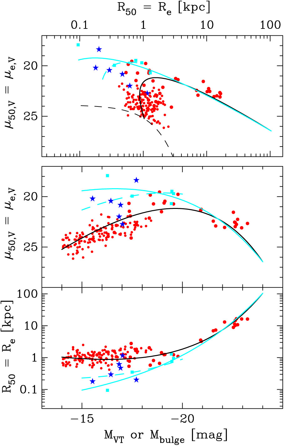
7. Discussion
7.1.
$\mathfrak{M}, \mu_{\rm e}$
, and
$R_{\rm e}$


Although Sérsic (Reference Sérsic1968b) plotted magnitude and mass versus $R_{\rm e}$
without yet fully appreciating the nature of ETGsFootnote cc, that is, how ETG light profiles systematically change shape with absolute magnitude, Sérsic (Reference Sérsic1968a) provided the very tool, that is, the
$R_{\rm e}$
without yet fully appreciating the nature of ETGsFootnote cc, that is, how ETG light profiles systematically change shape with absolute magnitude, Sérsic (Reference Sérsic1968a) provided the very tool, that is, the $R^{1/n}$
modelFootnote dd, that subsequently resulted in the realisation that the curved distribution of ETGs in diagrams using
$R^{1/n}$
modelFootnote dd, that subsequently resulted in the realisation that the curved distribution of ETGs in diagrams using $R_{\rm e}$
, or the associated
$R_{\rm e}$
, or the associated $\mu_{\rm e}$
and
$\mu_{\rm e}$
and
 $\langle \mu
\rangle_{\rm e}$
, is a consequence of the continual change in the Sérsic index n with absolute magnitude.
$\langle \mu
\rangle_{\rm e}$
, is a consequence of the continual change in the Sérsic index n with absolute magnitude.
Both Sérsic (Reference Sérsic1968b) and Fish (Reference Fish1963) deserve more recognition than received to date. Their ( $R_{\rm e}$
-based size)-luminosity (and size-mass) relations are the linear approximation to the bright arm of the curved size–luminosity relation for ETGs (see Graham et al. Reference Graham, Merritt, Moore, Diemand and Terzić2006) that is still fit by countless papers today (e.g. Shen et al. Reference Shen, Mo and White2003; Lange et al., Reference Lange, Driver and Robotham2015). As noted earlier, this linear approximation from half a century ago also simultaneously yields the linear approximation to the bright arm of both the
$R_{\rm e}$
-based size)-luminosity (and size-mass) relations are the linear approximation to the bright arm of the curved size–luminosity relation for ETGs (see Graham et al. Reference Graham, Merritt, Moore, Diemand and Terzić2006) that is still fit by countless papers today (e.g. Shen et al. Reference Shen, Mo and White2003; Lange et al., Reference Lange, Driver and Robotham2015). As noted earlier, this linear approximation from half a century ago also simultaneously yields the linear approximation to the bright arm of both the
 $\langle \mu
\rangle_{\rm e}$
–
$\langle \mu
\rangle_{\rm e}$
– $R_{\rm e}$
relation and the
$R_{\rm e}$
relation and the $\mu_{\rm e}$
–
$\mu_{\rm e}$
– $R_{\rm e}$
relation, which later became known as the Kormendy (Reference Kormendy1977) relation after Kormendy was the first to plot
$R_{\rm e}$
relation, which later became known as the Kormendy (Reference Kormendy1977) relation after Kormendy was the first to plot $\mu_{\rm e}$
versus
$\mu_{\rm e}$
versus $R_{\rm e}$
.
$R_{\rm e}$
.
Like previous papers, Kormendy (Reference Kormendy1977) used de Vaucouleurs’ $R^{1/4}$
model to parameterise the galaxy sample and wrote ‘some experimentation suggests that the most relevant correlation is between
$R^{1/4}$
model to parameterise the galaxy sample and wrote ‘some experimentation suggests that the most relevant correlation is between $B_{0V}$
[
$B_{0V}$
[ $\mu_{\rm e}$
] and
$\mu_{\rm e}$
] and $r_0$
[
$r_0$
[ $R_{\rm e}$
]’ and that ‘the interpretation of the
$R_{\rm e}$
]’ and that ‘the interpretation of the $B_{0V}(\log\, r_0)$
[
$B_{0V}(\log\, r_0)$
[ $\mu_{\rm e}$
–
$\mu_{\rm e}$
– $\log R_{\rm e}$
] is unknown’. As with Fish (Reference Fish1963), he had found that the B-band effective surface brightness was not constant among the ETG population. For luminous ETGs, Kormendy (Reference Kormendy1977) reported that
$\log R_{\rm e}$
] is unknown’. As with Fish (Reference Fish1963), he had found that the B-band effective surface brightness was not constant among the ETG population. For luminous ETGs, Kormendy (Reference Kormendy1977) reported that $\mu_{\rm e} \propto 3\log R_{\rm e}$
over a range of 3.5 mag arcsec-2. Although the following papers did not fit a curved relation, the more complete curved distribution for ETGs can be seen in Kodaira et al. (Reference Kodaira, Okamura and Watanabe1983), Ichikawa et al. (Reference Ichikawa, Wakamatsu and Okamura1986), and Capaccioli & Caon (Reference Capaccioli and Caon1991; see also Binggeli et al. Reference Binggeli, Sandage and Tarenghi1984 in regard to the curved
$\mu_{\rm e} \propto 3\log R_{\rm e}$
over a range of 3.5 mag arcsec-2. Although the following papers did not fit a curved relation, the more complete curved distribution for ETGs can be seen in Kodaira et al. (Reference Kodaira, Okamura and Watanabe1983), Ichikawa et al. (Reference Ichikawa, Wakamatsu and Okamura1986), and Capaccioli & Caon (Reference Capaccioli and Caon1991; see also Binggeli et al. Reference Binggeli, Sandage and Tarenghi1984 in regard to the curved $\mathfrak{M}_B$
–
$\mathfrak{M}_B$
– $\langle \mu \rangle _{\rm e}$
distribution). As interpretted/explained here, the
$\langle \mu \rangle _{\rm e}$
distribution). As interpretted/explained here, the $\mu_{\rm e}$
–
$\mu_{\rm e}$
– $R_{\rm e}$
and
$R_{\rm e}$
and $\langle \mu \rangle_{\rm e}$
–
$\langle \mu \rangle_{\rm e}$
– $R_{\rm e}$
relations for bright ETGs are tight because ETGs with Sérsic
$R_{\rm e}$
relations for bright ETGs are tight because ETGs with Sérsic $n\mathbin{\lower.3ex\hbox{$\buildrel\gt\over
{\smash{\scriptstyle\sim}\vphantom{_x}}$}} 3$
have similar (near over-lapping) light profiles. As such, errors in
$n\mathbin{\lower.3ex\hbox{$\buildrel\gt\over
{\smash{\scriptstyle\sim}\vphantom{_x}}$}} 3$
have similar (near over-lapping) light profiles. As such, errors in $R_{\rm e}$
, and thus
$R_{\rm e}$
, and thus $\mu_{\rm e}$
and
$\mu_{\rm e}$
and $\langle \mu \rangle_{\rm e}$
, shift bright ETGs of a given magnitude along these near over-lapping light profiles, maintaining a
$\langle \mu \rangle_{\rm e}$
, shift bright ETGs of a given magnitude along these near over-lapping light profiles, maintaining a $\mu_{\rm e}$
–
$\mu_{\rm e}$
– $R_{\rm e}$
and
$R_{\rm e}$
and $\langle \mu \rangle_{\rm e}$
–
$\langle \mu \rangle_{\rm e}$
– $R_{\rm e}$
relation that resembles the
$R_{\rm e}$
relation that resembles the $\mu$
–R and
$\mu$
–R and $\langle \mu \rangle$
–R light profiles (see Figure 5).
$\langle \mu \rangle$
–R light profiles (see Figure 5).
We have seen why fainter ETGs, with progressively different light profiles, smoothly depart from the $\mu_{\rm e}$
–
$\mu_{\rm e}$
– $R_{\rm e}$
and
$R_{\rm e}$
and $\langle \mu \rangle_{\rm e}$
–
$\langle \mu \rangle_{\rm e}$
– $R_{\rm e}$
relations for bright ETGs. (see Figure 5) reveals why Ichikawa et al. (Reference Ichikawa, Wakamatsu and Okamura1986) were mistaken when they interpreted the curved
$R_{\rm e}$
relations for bright ETGs. (see Figure 5) reveals why Ichikawa et al. (Reference Ichikawa, Wakamatsu and Okamura1986) were mistaken when they interpreted the curved $\mu_{\rm e}$
–
$\mu_{\rm e}$
– $R_{\rm e}$
distribution, see their Figure 12, as strong evidence for a separation of dwarf and giant ETGs; and half of the answer as to why they were mistaken is evident in their linear
$R_{\rm e}$
distribution, see their Figure 12, as strong evidence for a separation of dwarf and giant ETGs; and half of the answer as to why they were mistaken is evident in their linear $\mathfrak{M}_B$
–concentration relation (see their Figure 11). However, they were in good company, following Michard (Reference Michard1979), and their data quality and trends appear accurate.
$\mathfrak{M}_B$
–concentration relation (see their Figure 11). However, they were in good company, following Michard (Reference Michard1979), and their data quality and trends appear accurate.
It should also be borne in mind that any continuum can be split into two, but this does not mean that one has two distinct populations. For example, the colours of ETGs become more blue as one progresses to fainter magnitudesFootnote ae (e.g. Baum Reference Baum1959; Visvanathan & Sandage Reference Visvanathan and Sandage1977; Driver et al., Reference Driver, Allen and Graham2006; Lee, Lee, & Hwang, Reference Lee, Lee and Hwang2006; Bamford et al. Reference Bamford, Nichol and Baldry2009; Deng et al. Reference Deng, He, Wu and Ding2009; Kannappan, Guie, &Baker, Reference Kannappan, Guie and Baker2009), and one could construct a red and blue bin with a divide at say $\mathfrak{M}_B=-18$
mag. Furthermore, a histogram would appear bimodal if one excluded the bridging population from the sample, but this would not be evidence against a single unified population but rather evidence of sample selection. Similarly, the observation (Figure 1) that ETGs fainter than
$\mathfrak{M}_B=-18$
mag. Furthermore, a histogram would appear bimodal if one excluded the bridging population from the sample, but this would not be evidence against a single unified population but rather evidence of sample selection. Similarly, the observation (Figure 1) that ETGs fainter than $\mathfrak{M}_B=-18$
mag tend to have Sérsic indices
$\mathfrak{M}_B=-18$
mag tend to have Sérsic indices $n\lt2$
(exponential-like), while brighter ETGs tend to have
$n\lt2$
(exponential-like), while brighter ETGs tend to have $n>2$
(
$n>2$
( $R^{1/4}$
-like), is not evidence for two distinct populations. Similar caution is required for bulges.
$R^{1/4}$
-like), is not evidence for two distinct populations. Similar caution is required for bulges.
7.2.
$\mathfrak{M}$
–
$\mu_0$


This section contains a summary of past efforts to provide a physical explanation for the artificial dichotomy at $\mathfrak{M}_B = -18$
mag. Of course, as seen above, there is no division of ETGs at
$\mathfrak{M}_B = -18$
mag. Of course, as seen above, there is no division of ETGs at $\mathfrak{M}_B = -18$
mag.
$\mathfrak{M}_B = -18$
mag.
Some further historical context surrounding the $\mathfrak{M}$
–
$\mathfrak{M}$
– $\mu_0$
diagram should prove helpful and insightful.
$\mu_0$
diagram should prove helpful and insightful.
While de Vaucouleurs’ (Reference de Vaucouleurs1948, Reference de Vaucouleurs1953, Reference de Vaucouleurs and Flügge1959) $R^{1/4}$
model for describing bright ETGs, and the bulges of disc galaxies, took hold, Hodge (Reference Hodge1961a,b) had shown that de Vaucouleurs’ model did not provide a good description of the faint ETGs. Hodge, Pyper, & Webb (Reference Hodge, Pyper and Webb1965) noted, in the concluding sentence of their article, that all of their dwarf ETGs displayed an exponentialFootnote af light profile, as was shown in their Figures 4a–e. The influential article by Hodge (Reference Hodge1971) also reported that the exponential model works well for the barred dwarf Im galaxy IC 1613, see also de Vaucouleurs (Reference de Vaucouleurs1961a) for other Irregular galaxies. This engendered suspicions of a connection between the discs at one end of the Aitken–Jeans–Lundmark–Hubble sequence and faint ETGs at the other. Faber & Lin (Reference Faber and Lin1983) and Binggeli et al. (Reference Binggeli, Sandage and Tarenghi1984) continued to show that the exponential model provides a reasonable description of the light profiles of faint ETGs. Kormendy (Reference Kormendy1985) subsequently added two generic disc galaxies from Freeman (Reference Freeman1970) into his
$R^{1/4}$
model for describing bright ETGs, and the bulges of disc galaxies, took hold, Hodge (Reference Hodge1961a,b) had shown that de Vaucouleurs’ model did not provide a good description of the faint ETGs. Hodge, Pyper, & Webb (Reference Hodge, Pyper and Webb1965) noted, in the concluding sentence of their article, that all of their dwarf ETGs displayed an exponentialFootnote af light profile, as was shown in their Figures 4a–e. The influential article by Hodge (Reference Hodge1971) also reported that the exponential model works well for the barred dwarf Im galaxy IC 1613, see also de Vaucouleurs (Reference de Vaucouleurs1961a) for other Irregular galaxies. This engendered suspicions of a connection between the discs at one end of the Aitken–Jeans–Lundmark–Hubble sequence and faint ETGs at the other. Faber & Lin (Reference Faber and Lin1983) and Binggeli et al. (Reference Binggeli, Sandage and Tarenghi1984) continued to show that the exponential model provides a reasonable description of the light profiles of faint ETGs. Kormendy (Reference Kormendy1985) subsequently added two generic disc galaxies from Freeman (Reference Freeman1970) into his $\mathfrak{M}_B$
–
$\mathfrak{M}_B$
– $\mu_0$
diagram, to represent dwarf Irregular and late-type spiral galaxies near the bright-end of his skewed dwarf ETG distribution; see also K09 (their Figure 1) and Tolstoy et al. (Reference Tolstoy, Hill and Tosi2009, their Figure 1). Kormendy (Reference Kormendy1985) then went on to advocate that dwarf elliptical (dE) galaxies are better connected with the dwarf spiral and dwarf irregular galaxies found at the other end of the Aitken–Jeans–Lundmark–Hubble sequence and do not connect with ordinary ETGs at
$\mu_0$
diagram, to represent dwarf Irregular and late-type spiral galaxies near the bright-end of his skewed dwarf ETG distribution; see also K09 (their Figure 1) and Tolstoy et al. (Reference Tolstoy, Hill and Tosi2009, their Figure 1). Kormendy (Reference Kormendy1985) then went on to advocate that dwarf elliptical (dE) galaxies are better connected with the dwarf spiral and dwarf irregular galaxies found at the other end of the Aitken–Jeans–Lundmark–Hubble sequence and do not connect with ordinary ETGs at $\mathfrak{M}_B = -18$
mag. This view differed from Sandage & Binggeli (Reference Sandage and Binggeli1984, see their Figure 1) who suggested a strong connection between dE and E galaxies, and a weak connection between dE and dwarf Irregular/Magellanic-like galaxies. In addition, Wirth & Gallagher (Reference Wirth and Gallagher1984) had just suggested that compact elliptical (cE) galaxies (de Vaucouleurs Reference de Vaucouleurs1961b; Zwicky & Kowal Reference Zwicky and Kowal1968; Zwicky & Zwicky Reference Zwicky and Zwicky1971) rather than dwarf ETGs may be the low-luminosity analogs of ordinary ETGs. Indeed, Fish (Reference Fish1963) had also noted that M32 defined the faint-end of his size–luminosity relation for elliptical galaxies, and K09 maintains this view.
$\mathfrak{M}_B = -18$
mag. This view differed from Sandage & Binggeli (Reference Sandage and Binggeli1984, see their Figure 1) who suggested a strong connection between dE and E galaxies, and a weak connection between dE and dwarf Irregular/Magellanic-like galaxies. In addition, Wirth & Gallagher (Reference Wirth and Gallagher1984) had just suggested that compact elliptical (cE) galaxies (de Vaucouleurs Reference de Vaucouleurs1961b; Zwicky & Kowal Reference Zwicky and Kowal1968; Zwicky & Zwicky Reference Zwicky and Zwicky1971) rather than dwarf ETGs may be the low-luminosity analogs of ordinary ETGs. Indeed, Fish (Reference Fish1963) had also noted that M32 defined the faint-end of his size–luminosity relation for elliptical galaxies, and K09 maintains this view.
With the availability of better spatially resolved data from the HST, Kormendy et al. (Reference Kormendy, Dressler and Byun1994, see also Ferrarese et al., Reference Ferrarese, van den Bosch, Ford, Jaffe and O’Connell1994 and Grillmair et al., Reference Grillmair, Faber and Lauer1994) used the $R^{1/4}$
model to describe the global properties of galaxies, and a double power-law modelFootnote ag to describe their inner region. In order to measure the host galaxy light, they appropriately advocated for excluding the additional nuclear components (common in both dwarf and ordinary ETGs, and LTGs: e.g. Rest et al. Reference Rest, van den Bosch and Jaffe2001; Balcells et al. Reference Balcells, Graham, Domínguez-Palmero and Peletier2003; Böker et al. Reference Böker, Sarzi and McLaughlin2004), as can be seen in the light profiles shown by Lauer et al. (Reference Lauer, Ajhar and Byun1995), Byun et al. (Reference Byun, Grillmair and Faber1996), and later K09. While the HST data revealed that it was galaxies with partially depleted cores that were deviating from the
$R^{1/4}$
model to describe the global properties of galaxies, and a double power-law modelFootnote ag to describe their inner region. In order to measure the host galaxy light, they appropriately advocated for excluding the additional nuclear components (common in both dwarf and ordinary ETGs, and LTGs: e.g. Rest et al. Reference Rest, van den Bosch and Jaffe2001; Balcells et al. Reference Balcells, Graham, Domínguez-Palmero and Peletier2003; Böker et al. Reference Böker, Sarzi and McLaughlin2004), as can be seen in the light profiles shown by Lauer et al. (Reference Lauer, Ajhar and Byun1995), Byun et al. (Reference Byun, Grillmair and Faber1996), and later K09. While the HST data revealed that it was galaxies with partially depleted cores that were deviating from the $\mathfrak{M}_B$
–
$\mathfrak{M}_B$
– $\mu_0$
relation defined by ordinary ETGs without cores — as previously reported by Oemler (1973) and Gudehus (Reference Gudehus1973) — Faber et al. (Reference Faber, Tremaine and Ajhar1997) claimed that if they had even better spatial resolution then they would obtain brighter central surface brightnesses for those ETGs without cores in the magnitude range
$\mu_0$
relation defined by ordinary ETGs without cores — as previously reported by Oemler (1973) and Gudehus (Reference Gudehus1973) — Faber et al. (Reference Faber, Tremaine and Ajhar1997) claimed that if they had even better spatial resolution then they would obtain brighter central surface brightnesses for those ETGs without cores in the magnitude range $-18 > \mathfrak{M}_B > -20.5$
mag, thereby uniting the core-Sérsic and Sérsic galaxies with a linear relation in the
$-18 > \mathfrak{M}_B > -20.5$
mag, thereby uniting the core-Sérsic and Sérsic galaxies with a linear relation in the $\mathfrak{M}$
–
$\mathfrak{M}$
– $\mu_0$
diagram and separating them from the dwarf ETGs. Faber et al. (Reference Faber, Tremaine and Ajhar1997, see their Figure 4) used the nearby, nucleated, Sérsic galaxy M32 as an example of this, including the nuclear star cluster in order to report the higher surface brightness required to make this galaxy follow the
$\mu_0$
diagram and separating them from the dwarf ETGs. Faber et al. (Reference Faber, Tremaine and Ajhar1997, see their Figure 4) used the nearby, nucleated, Sérsic galaxy M32 as an example of this, including the nuclear star cluster in order to report the higher surface brightness required to make this galaxy follow the $\mathfrak{M}_B$
–
$\mathfrak{M}_B$
– $\mu_0$
relation defined by the luminous ETGs with depleted cores. This was, however, at odds with their treatment of other galaxies where they excluded additional nuclear components from the modelling process and obviously meant that they were no longer working with the properties of the host galaxy but were subject to the whims of nuclear star cluster formation.
$\mu_0$
relation defined by the luminous ETGs with depleted cores. This was, however, at odds with their treatment of other galaxies where they excluded additional nuclear components from the modelling process and obviously meant that they were no longer working with the properties of the host galaxy but were subject to the whims of nuclear star cluster formation.
Please provide the expansion for “CCD”,if needed.Combining CCD images with deep, wide field-of-view, photographic data (Caon et al. (Reference Caon, Capaccioli and D’Onofrio1993) and D’Onofrio et al. (Reference D’Onofrio, Capaccioli and Caon1994)) had shown that the Sérsic function fits the brightness profiles of ETGs remarkably well over a large dynamic range. Graham & Guzmán (Reference Graham and Guzmán2003) and Balcells et al. (Reference Balcells, Graham, Domínguez-Palmero and Peletier2003) used the Sérsic $R^{1/n}$
model to quantify HST-resolved galaxies and bulges. In addition, they simultaneously modelled the galaxy’s discs and nuclear components, while Graham et al. (Reference Graham, Erwin, Trujillo and Asensio Ramos2003) showed how to unite the inner and outer regions of galaxies using the core-Sérsic model, rather than using a disconnected double power-law for the inner region and an
$R^{1/n}$
model to quantify HST-resolved galaxies and bulges. In addition, they simultaneously modelled the galaxy’s discs and nuclear components, while Graham et al. (Reference Graham, Erwin, Trujillo and Asensio Ramos2003) showed how to unite the inner and outer regions of galaxies using the core-Sérsic model, rather than using a disconnected double power-law for the inner region and an $R^{1/4}$
model for the outer region. Furthermore, unlike the double power-law model, the Sérsic
$R^{1/4}$
model for the outer region. Furthermore, unlike the double power-law model, the Sérsic $R^{1/n}$
model previously applied to core-less galaxies has a finite central surface brightness, useful for quantifying the host bulge/galaxy
$R^{1/n}$
model previously applied to core-less galaxies has a finite central surface brightness, useful for quantifying the host bulge/galaxy $\mu_0$
in galaxies without depleted cores, such as M32. Graham et al. (Reference Graham, Erwin, Trujillo and Asensio Ramos2003) and Balcells et al. (Reference Balcells, Graham, Domínguez-Palmero and Peletier2003) advocated the identification and quantification of both central deficits (partially depleted cores) and excesses (additional nuclear components) relative to the inward extrapolation of the bulge’s outer Sérsic profile, a practice later adopted by Ferrarese et al. Reference Ferrarese, Côté and Jordán2006 and K09Footnote hh. Graham & Guzmán (Reference Graham and Guzmán2003) revealed that the
$\mu_0$
in galaxies without depleted cores, such as M32. Graham et al. (Reference Graham, Erwin, Trujillo and Asensio Ramos2003) and Balcells et al. (Reference Balcells, Graham, Domínguez-Palmero and Peletier2003) advocated the identification and quantification of both central deficits (partially depleted cores) and excesses (additional nuclear components) relative to the inward extrapolation of the bulge’s outer Sérsic profile, a practice later adopted by Ferrarese et al. Reference Ferrarese, Côté and Jordán2006 and K09Footnote hh. Graham & Guzmán (Reference Graham and Guzmán2003) revealed that the $\mathfrak{M}_B$
–
$\mathfrak{M}_B$
– $\mu_0$
diagram displays no evidence for the alleged ETG divide at
$\mu_0$
diagram displays no evidence for the alleged ETG divide at $\mathfrak{M}_B \approx -18$
mag that had been advocated by Kormendy (Reference Kormendy1985), Faber et al. (Reference Faber, Tremaine and Ajhar1997), and in numerous papers since then (e.g. Kormendy Reference Kormendy, Laurikainen, Peletier and Gadotti2016, and references therein). Instead, Graham & Guzmán (Reference Graham and Guzmán2003) argued that the only magnitude of importance in this diagram is around
$\mathfrak{M}_B \approx -18$
mag that had been advocated by Kormendy (Reference Kormendy1985), Faber et al. (Reference Faber, Tremaine and Ajhar1997), and in numerous papers since then (e.g. Kormendy Reference Kormendy, Laurikainen, Peletier and Gadotti2016, and references therein). Instead, Graham & Guzmán (Reference Graham and Guzmán2003) argued that the only magnitude of importance in this diagram is around
 $\mathfrak{M}_B =
-20.5$
mag, corresponding to the division between ETGs whose spheroidal component had a Sérsic profile versus ETGs whose spheroidal component had a core-Sérsic profile. This magnitude corresponds to a mass of
$\mathfrak{M}_B =
-20.5$
mag, corresponding to the division between ETGs whose spheroidal component had a Sérsic profile versus ETGs whose spheroidal component had a core-Sérsic profile. This magnitude corresponds to a mass of
 $(1-2)\times
10^{11}\,{\rm M}_{\odot}$
.
$(1-2)\times
10^{11}\,{\rm M}_{\odot}$
.
7.3. Formation scenarios
It had become common to see papers refer to supernova-driven winds as the physical explanation for creating two disconnected species of ETG, with the winds blowing the gas out of the dwarf galaxies (e.g. Mathews & Baker Reference Mathews and Baker1971; Saito Reference Saito1979) and making them different to ordinary ETGs. Dekel & Silk (Reference Dekel and Silk1986) invoked supernova-driven winds for creating the two distinct classes of galaxies thought to have been observed in their $\mathfrak{M}_B$
–
$\mathfrak{M}_B$
– $\langle \mu \rangle_{\rm e}$
diagram. However, these studies over-looked the gravitational-binding energy of the dark matter halo (Mac Low & Ferrara Reference Mac Low and Ferrara1999)Footnote ii. A mechanism other than winds was therefore sought to explain the alleged discontinuity at
$\langle \mu \rangle_{\rm e}$
diagram. However, these studies over-looked the gravitational-binding energy of the dark matter halo (Mac Low & Ferrara Reference Mac Low and Ferrara1999)Footnote ii. A mechanism other than winds was therefore sought to explain the alleged discontinuity at $\mathfrak{M}_B \approx -18$
mag.
$\mathfrak{M}_B \approx -18$
mag.
The claim that dwarf ETGs are formed from dIrrs had been challenged by Bothun et al. (Reference Bothun, Mould, Caldwell and MacGillivray1986; see also Hunter & Gallagher Reference Hunter and Gallagher1985, their Figure 12), who reported that the irregular galaxies did not have the right magnitudes, surface brightnesses, nor colours, to evolve into dE galaxies. Investigating the structure of dwarf galaxies at near-infrared wavelengths, which are less affected by dust and the light from new stars, James (Reference James1991); James (Reference James1994) similarly concluded that the dwarf Irr and dwarf ETGs differ markedly and it is unlikely that dwarf Irr galaxies transform into dwarf ETGs. Nonetheless, given the notion that ordinary elliptical galaxies formed from the merger of spiral galaxies (e.g. Toomre & Toomre Reference Toomre and Toomre1972), one can appreciate why the dwarf ETG population may have been suspected to have been morphologically transformed from something else. The absence of enough sufficiently low mass spiral galaxies (e.g. Sandage & Binggeli Reference Sandage and Binggeli1984) that could merge and build the dwarf ETG population led to thoughts of yet alternative processes. Shapley (Reference Shapley1951) had previously suggested that the Small Magellanic Cloud may be evolving into a dE galaxy, and Einasto et al. (Reference Einasto, Saar, Kaasik and Chernin1974), Frogel et al. (Reference Frogel, Blanco, McCarthy and Cohen1982), Faber & Lin (Reference Faber and Lin1983), Lin & Faber (Reference Lin and Faber1983), Wirth & Gallagher (Reference Wirth and Gallagher1984), and others similarly suggested that removing the gas content from a dwarf irregular galaxy may produce a dE galaxy; after all, they both had exponential light profiles.
Influenced by the shape of the light profile, there were speculations that the dwarf ETGs were associated with flat discs. However, the dEs were later shown to be ellipsoidal or at least not disc-like (e.g. Ichikawa et al. Reference Ichikawa, Wakamatsu and Okamura1986). That is, an exponential-like (Sérsic $n=1$
) light profile does not necessarily imply a flat disc. Chen et al. (Reference Chen, Côté, West, Peng and Ferrarese2010) wrote that ‘The distribution of axial ratios of low-mass (‘dwarf’) galaxies bears a strong resemblance to the one observed for the higher-mass (‘giant’) galaxies’. Therefore, removing the gas from late-type spiral and Irregular galaxies, via the ram-pressure stripping from a galaxy cluster’s hot X-ray gas, was not enough to explain the alleged (dwarf ETG) – (Irregular galaxy) connection. In passing, it is noted that ETGs can contain substantial discs, but as a population, they do not have the abundance of low bulge-to-total ratios as seen in late-type spiral and irregular galaxies.
$n=1$
) light profile does not necessarily imply a flat disc. Chen et al. (Reference Chen, Côté, West, Peng and Ferrarese2010) wrote that ‘The distribution of axial ratios of low-mass (‘dwarf’) galaxies bears a strong resemblance to the one observed for the higher-mass (‘giant’) galaxies’. Therefore, removing the gas from late-type spiral and Irregular galaxies, via the ram-pressure stripping from a galaxy cluster’s hot X-ray gas, was not enough to explain the alleged (dwarf ETG) – (Irregular galaxy) connection. In passing, it is noted that ETGs can contain substantial discs, but as a population, they do not have the abundance of low bulge-to-total ratios as seen in late-type spiral and irregular galaxies.
Moore et al. (Reference Moore, Katz, Lake, Dressler and Oemler1996) subsequently revealed how multiple fast fly-bys past a massive perturbing galaxy, coupled with gravitational tidal forces within a galaxy cluster, could first invoke the formation of a bar within a small low-mass (Sd-like) disc galaxy and then strip away the remaining outer disc, leaving behind a somewhat harassed and puffed-up bar that was proposed to be the answer to the existence of dwarf ETGs and the lower-mass dSph galaxies in clusters. This mechanism maintained the suspected association with spiral galaxies and removed the connection with brighter ETGs. However, while the galaxy harassment scenario (Moore et al. Reference Moore, Katz, Lake, Dressler and Oemler1996; Moore et al. Reference Moore, Lake and Katz1998; Mastropietro et al. Reference Mastropietro, Moore and Mayer2005, see also Mayer et al. Reference Mayer, Governato and Colpi2001a; Mayer et al. Reference Mayer, Governato and Colpi2001b) likely transforms low mass disc galaxies, it is unlikely to be capable of creating ETGs with $\mathfrak{M}_B = -16$
to
$\mathfrak{M}_B = -16$
to $-18$
mag by stripping away much more luminous spiral galaxies. Moreover, a population of dynamically heated, but still rather flat, bars has not been observed in galaxy clusters. Instead, the dwarf ETGs are a population of multi-component galaxies possessing features that ordinary (
$-18$
mag by stripping away much more luminous spiral galaxies. Moreover, a population of dynamically heated, but still rather flat, bars has not been observed in galaxy clusters. Instead, the dwarf ETGs are a population of multi-component galaxies possessing features that ordinary (
 $\mathfrak{M}_B
\mathbin{\lower.3ex\hbox{$\buildrel\lt\over
{\smash{\scriptstyle\sim}\vphantom{_x}}$}} -18$
mag) ETGs, not thought to have been built by stripping/harassing of spiral galaxies, also contain. The existence of isolated dwarf ETGs, shown to have the same kinematic properties as dwarf ETGs in clusters (Janz et al. Reference Janz, Penny, Graham, Forbes and Davies2017; Graham et al. Reference Graham, Janz and Penny2017), reveals that dwarf ETGs need not have been built by ‘galaxy harassment’. They are thus built by Nature rather than Nurture: they do not require the harsh (nurturing) environment of a galaxy cluster to form.
$\mathfrak{M}_B
\mathbin{\lower.3ex\hbox{$\buildrel\lt\over
{\smash{\scriptstyle\sim}\vphantom{_x}}$}} -18$
mag) ETGs, not thought to have been built by stripping/harassing of spiral galaxies, also contain. The existence of isolated dwarf ETGs, shown to have the same kinematic properties as dwarf ETGs in clusters (Janz et al. Reference Janz, Penny, Graham, Forbes and Davies2017; Graham et al. Reference Graham, Janz and Penny2017), reveals that dwarf ETGs need not have been built by ‘galaxy harassment’. They are thus built by Nature rather than Nurture: they do not require the harsh (nurturing) environment of a galaxy cluster to form.
The presence of disc-like features (e.g. Graham et al. Reference Graham, Jerjen and Guzmán2003b; Lisker et al. Reference Lisker, Grebel and Binggeli2006; Lisker & Fuchs Reference Lisker and Fuchs2009) and rotation in dwarf ETGs in clusters — known since Davies et al. (Reference Davies, Efstathiou, Fall, Illingworth and Schechter1983) — had been heralded as evidence that they were previously spiral galaxies (e.g. Boselli et al. Reference Boselli, Boissier, Cortese and Gavazzi2008; De Rijcke et al. Reference De Rijcke, Van Hese and Buyle2010; Penny et al. Reference Penny, Forbes, Pimbblet and Floyd2014; Ryś $\mathfrak{M}$
et al. 2015; Toloba et al. Reference Toloba, Guhathakurta and Boselli2015), even though ordinary ETGs display the very same features. Such discs, observed in ETGs up to
$\mathfrak{M}$
et al. 2015; Toloba et al. Reference Toloba, Guhathakurta and Boselli2015), even though ordinary ETGs display the very same features. Such discs, observed in ETGs up to $\sim 10^{11}\,{\rm M}_{\odot}$
(e.g. Emsellem et al. Reference Emsellem, Cappellari and Krajnović2011; Krajnavić et al. Reference Krajnović, Alatalo and Blitz2013), may be built from gas accretion and minor mergers (e.g. Schweizer Reference Schweizer1986; Schweizer & Seitzer Reference Schweizer and Seitzer1988; Birnboim & Dekel Reference Birnboim and Dekel2003; Katz et al. Reference Katz, Keres, Dave and Weinberg2003; Mei et al. Reference Mei, Blakeslee and Stanford2006; Wei et al. Reference Wei, Kannappan, Vogel and Baker2010; Kaviraj et al. Reference Kaviraj, Tan, Ellis and Silk2011). Structurally and kinematically, dwarf and ordinary ETGs (both in and out of clusters) display a continuum of disc-like features across the alleged divide at
$\sim 10^{11}\,{\rm M}_{\odot}$
(e.g. Emsellem et al. Reference Emsellem, Cappellari and Krajnović2011; Krajnavić et al. Reference Krajnović, Alatalo and Blitz2013), may be built from gas accretion and minor mergers (e.g. Schweizer Reference Schweizer1986; Schweizer & Seitzer Reference Schweizer and Seitzer1988; Birnboim & Dekel Reference Birnboim and Dekel2003; Katz et al. Reference Katz, Keres, Dave and Weinberg2003; Mei et al. Reference Mei, Blakeslee and Stanford2006; Wei et al. Reference Wei, Kannappan, Vogel and Baker2010; Kaviraj et al. Reference Kaviraj, Tan, Ellis and Silk2011). Structurally and kinematically, dwarf and ordinary ETGs (both in and out of clusters) display a continuum of disc-like features across the alleged divide at $\mathfrak{M}_B = -18$
mag.
$\mathfrak{M}_B = -18$
mag.
As Tolstoy et al. (Reference Tolstoy, Hill and Tosi2009) note, in their Introduction’s third paragraph, dwarf galaxies ( $\mathfrak{M}_B > - 16$
mag) form a continuum with brighter non-dwarf galaxies, in terms of potential well, size, structural, kinematic, and population features. Indeed, the dwarf and ordinary ETGs follow a continuous luminosity–metallicity relation (Dekel & Silk Reference Dekel and Silk1986, see their Figure 2; Mateo Reference Mateo1998; Tremonti et al. Reference Tremonti, Heckman and Kauffmann2004; Veilleux et al. Reference Veilleux, Cecil and Bland-Hawthorn2005) which the Sm-Irr galaxies do not follow: the latter are less metal-rich than dwarf ETGs of the same luminosity (Mateo Reference Mateo1998; Grebel 2004). In addition, the L–
$\mathfrak{M}_B > - 16$
mag) form a continuum with brighter non-dwarf galaxies, in terms of potential well, size, structural, kinematic, and population features. Indeed, the dwarf and ordinary ETGs follow a continuous luminosity–metallicity relation (Dekel & Silk Reference Dekel and Silk1986, see their Figure 2; Mateo Reference Mateo1998; Tremonti et al. Reference Tremonti, Heckman and Kauffmann2004; Veilleux et al. Reference Veilleux, Cecil and Bland-Hawthorn2005) which the Sm-Irr galaxies do not follow: the latter are less metal-rich than dwarf ETGs of the same luminosity (Mateo Reference Mateo1998; Grebel 2004). In addition, the L– $\sigma$
relation reveals unity rather than division among the ETGs at
$\sigma$
relation reveals unity rather than division among the ETGs at $\mathfrak{M}_B = -18$
mag, with a continuous log-linear relation, having a slope of 2 in the B-band, which encompasses ETGs with
$\mathfrak{M}_B = -18$
mag, with a continuous log-linear relation, having a slope of 2 in the B-band, which encompasses ETGs with $\mathfrak{M}_B \mathbin{\lower.3ex\hbox{$\buildrel\gt\over
{\smash{\scriptstyle\sim}\vphantom{_x}}$}} -20.5$
mag (Davies et al. Reference Davies, Efstathiou, Fall, Illingworth and Schechter1983; Matković
$\mathfrak{M}$
& Guzmán 2005; Hyde and Bernardi Reference Hyde and Bernardi2009; Graham & Soria Reference Graham and Soria2019, see their Figure 1).
$\mathfrak{M}_B \mathbin{\lower.3ex\hbox{$\buildrel\gt\over
{\smash{\scriptstyle\sim}\vphantom{_x}}$}} -20.5$
mag (Davies et al. Reference Davies, Efstathiou, Fall, Illingworth and Schechter1983; Matković
$\mathfrak{M}$
& Guzmán 2005; Hyde and Bernardi Reference Hyde and Bernardi2009; Graham & Soria Reference Graham and Soria2019, see their Figure 1).
7.4. Bulges and discs
A large fraction of ETGs contain discs. Careful image analysis had previously revealed overlooked discs in many ETGs (e.g. Capaccioli, Reference Capaccioli1987), and subsequent kinematic studies revealed the prevalence of discs in ETGs (e.g. D’Onofrio et al. Reference D’Onofrio, Zaggia, Longo, Caon and Capaccioli1995; Graham et al. Reference Graham, Colless, Busarello, Zaggia and Longo1998; Pedraz et al. Reference Pedraz, Gorgas, Cardiel, Sánchez-Blázquez and Guzmán2002; Emsellem et al. Reference Emsellem, Cappellari and Krajnović2011; Scott et al. Reference Scott, Davies and Houghton2014). In addition, modern structural decompositions reveal multiple physicalFootnote jj components in ETGs (e.g. Prieto et al. Reference Prieto, Aguerri, Varela and Muñoz-Tuñón2001; Läsker et al. Reference Läsker, Ferrarese and van de Ven2014; Savorgnan & Graham, Reference Savorgnan and Graham2016; Sahu et al. Reference Sahu, Graham and Davis2019). Nowadays, in such studies, Sérsic’s model provides an accurate description of the spheroidal component of the galaxy. In some instances, this is the entire galaxy, but ETGs less luminous than $\mathfrak{M}_B \approx -20.5$
mag invariably contain a disc, and sometimes a bar, ring, ansae, nuclear star cluster, or a more extended nuclear disc (e.g. de Vaucouleurs et al. Reference de Vaucouleurs, de Vaucouleurs, Corwin, Buta, Paturel and Fouqué1991; Ferrarese et al. Reference Ferrarese, Côté and Jordán2006; Saha et al. 2019). Not surprisingly, those studying galaxy structures have presented the
$\mathfrak{M}_B \approx -20.5$
mag invariably contain a disc, and sometimes a bar, ring, ansae, nuclear star cluster, or a more extended nuclear disc (e.g. de Vaucouleurs et al. Reference de Vaucouleurs, de Vaucouleurs, Corwin, Buta, Paturel and Fouqué1991; Ferrarese et al. Reference Ferrarese, Côté and Jordán2006; Saha et al. 2019). Not surprisingly, those studying galaxy structures have presented the $\mathfrak{M}$
–
$\mathfrak{M}$
– $\log\, n$
and
$\log\, n$
and $\mathfrak{M}$
–
$\mathfrak{M}$
– $\mu_0$
relations for bulges and observed the offset from ETGs (e.g. Andredakis et al. Reference Andredakis, Peletier and Balcells1995; Khosroshahi et al. Reference Khosroshahi, Wadadekar and Kembhavi2000; Graham Reference Graham2001; Möllenhoff & Heidt Reference Möllenhoff and Heidt2001; MacArthur et al. Reference MacArthur, Courteau and Holtzman2003).
$\mu_0$
relations for bulges and observed the offset from ETGs (e.g. Andredakis et al. Reference Andredakis, Peletier and Balcells1995; Khosroshahi et al. Reference Khosroshahi, Wadadekar and Kembhavi2000; Graham Reference Graham2001; Möllenhoff & Heidt Reference Möllenhoff and Heidt2001; MacArthur et al. Reference MacArthur, Courteau and Holtzman2003).
7.4.1 Galaxy Bulges and Red Nuggets
For well over a decade, the galaxy size–luminosity relation, or rather, the $R_{\rm e}$
–(stellar mass,
$R_{\rm e}$
–(stellar mass, $M_*$
) relation, has been used to argue that the compact (
$M_*$
) relation, has been used to argue that the compact ( $R_{\rm e} \mathbin{\lower.3ex\hbox{$\buildrel\lt\over
{\smash{\scriptstyle\sim}\vphantom{_x}}$}} 2$
kpc) massive (
$R_{\rm e} \mathbin{\lower.3ex\hbox{$\buildrel\lt\over
{\smash{\scriptstyle\sim}\vphantom{_x}}$}} 2$
kpc) massive ( $M_* \mathbin{\lower.3ex\hbox{$\buildrel\gt\over
{\smash{\scriptstyle\sim}\vphantom{_x}}$}} 10^{11}\,{\rm M}_{\odot}$
) spheroidal-shaped galaxies at high-redshifts (
$M_* \mathbin{\lower.3ex\hbox{$\buildrel\gt\over
{\smash{\scriptstyle\sim}\vphantom{_x}}$}} 10^{11}\,{\rm M}_{\odot}$
) spheroidal-shaped galaxies at high-redshifts ( $z\approx 2\pm1$
) — referred to as ‘red nuggets’ by Damjanov et al. (Reference Damjanov, McCarthy, Abraham, Glazebrook and Yan2009) — must have evolved into large massive elliptical galaxies in the local (
$z\approx 2\pm1$
) — referred to as ‘red nuggets’ by Damjanov et al. (Reference Damjanov, McCarthy, Abraham, Glazebrook and Yan2009) — must have evolved into large massive elliptical galaxies in the local ( $z=0$
) Universe (e.g. Daddi et al. Reference Daddi, Renzini, Pirzkal, Cimatti and Malhotra2005; Kriek et al. Reference Kriek, van Dokkum and Franx2006; Trujillo et al. Reference Trujillo, Förster Schreiber and Rudnick2006; van Dokkum 2008). The argument has been that dry merger events have increased the size of the three-dimensional spheroidal structures, building elliptical galaxies rather than lenticular galaxies with large-scale discs. However, most ETGs in the local universe contain fast-rotating two-dimensional discs. In many instances, it is the disc which makes these galaxies large.
$z=0$
) Universe (e.g. Daddi et al. Reference Daddi, Renzini, Pirzkal, Cimatti and Malhotra2005; Kriek et al. Reference Kriek, van Dokkum and Franx2006; Trujillo et al. Reference Trujillo, Förster Schreiber and Rudnick2006; van Dokkum 2008). The argument has been that dry merger events have increased the size of the three-dimensional spheroidal structures, building elliptical galaxies rather than lenticular galaxies with large-scale discs. However, most ETGs in the local universe contain fast-rotating two-dimensional discs. In many instances, it is the disc which makes these galaxies large.
Graham et al. Reference Graham, Dullo and Savorgnan2015 identified two dozen ‘compact massive spheroids’ as the bulge component of local lenticular galaxies. These bulges have the same distribution of sizes, masses, and Sérsic indices as the high-z compact massive galaxies and comparable number densities per unit volume of space (de la Rosa et al. Reference de la Rosa, La Barbera and Ferreras2016). This similarity strongly suggests that the above popular evolutionary scenario building bigger spheroids is not the complete picture. Rather, the evolution of these high-z red nuggets may instead be connected with the growth of discs (e.g. Caldwell 1983b; Morganti et al. Reference Morganti, de Zeeuw and Oosterloo2006; Sancisi et al. Reference Sancisi, Fraternali, Oosterloo and van der Hulst2008; Stewart et al. Reference Stewart, Bullock, Wechsler and Maller2009; Pichon et al. Reference Pichon, Pogosyan and Kimm2011; Moffett et al. Reference Moffett, Kannappan, Baker and Laine2012; Moffett et al. Reference Moffett, Kannappan and Berlind2015; Stark et al. Reference Stark, Kannappan and Wei2013; Graham et al. Reference Graham, Dullo and Savorgnan2015, see their Section 4.1; Kleiner et al. Reference Kleiner, Pimbblet, Jones, Koribalski and Serra2017). Gas accretion, both preceding and during ‘cosmic noon’, is expected to play a key role for the massive galaxies (Feldmann et al. Reference Feldmann, Hopkins, Quataert, Faucher-Giguère and Kereš2016), while the less massive galaxies, that is, smaller over-densities, take longer to accrete smaller quantities of gas in a ‘down-sizing’ (Cowie et al. Reference Cowie, Songaila, Hu and Cohen1996) scenario (Graham et al. Reference Graham, Dullo and Savorgnan2015; Graham et al. Reference Graham, Janz and Penny2017).
It is insightful to compare the two key empirical relations for ETGs (equations 16 and 17) with the equivalent relations for the bulges of S0 galaxies and LTGs. Graham & Worley (Reference Graham and Worley2008) compiled K-band data for the bulges of $\sim$
400 spiral and S0 galaxies, and Graham (Reference Graham, Oswalt and Keel2013) presented these two key equations for bulges (see his equations 2.19 and 2.20).Footnote kk They are such that
$\sim$
400 spiral and S0 galaxies, and Graham (Reference Graham, Oswalt and Keel2013) presented these two key equations for bulges (see his equations 2.19 and 2.20).Footnote kk They are such that
 \begin{eqnarray}
\mathfrak{M}_K &=& -7.5\log(n) - 20.0 \, {\rm and} \label{eqn36}\end{eqnarray}
\begin{eqnarray}
\mathfrak{M}_K &=& -7.5\log(n) - 20.0 \, {\rm and} \label{eqn36}\end{eqnarray}
 \begin{eqnarray}
\mathfrak{M}_K &=& 0.6\mu_{0,K} - 29.7.
\label{eqn37}\end{eqnarray}
\begin{eqnarray}
\mathfrak{M}_K &=& 0.6\mu_{0,K} - 29.7.
\label{eqn37}\end{eqnarray}
We can take a quick look at how ETGs and bulges compare using the following rough transformation. Given the current interest in compact massive spheroids, a simple $B-K$
colour of 4 and a stellar mass-to-light ratio of 8 are used for everything. The left panel in Figure 18 shows the
$B-K$
colour of 4 and a stellar mass-to-light ratio of 8 are used for everything. The left panel in Figure 18 shows the $\mathfrak{M}_B$
–
$\mathfrak{M}_B$
– $R_{\rm e}$
relation for the ETGs (as seen in Figure 4) and the expected
$R_{\rm e}$
relation for the ETGs (as seen in Figure 4) and the expected $\mathfrak{M}_B$
–
$\mathfrak{M}_B$
– $R_{\rm e}$
relation for bulges (using equations 36 and 37, and assuming
$R_{\rm e}$
relation for bulges (using equations 36 and 37, and assuming $B-K =4$
). Converting
$B-K =4$
). Converting $\mathfrak{M}_B$
into a stellar mass using
$\mathfrak{M}_B$
into a stellar mass using $\mathfrak{M}_{\odot,B} = 5.44$
mag (Mann & von Braun Reference Mann and von Braun2015) and
$\mathfrak{M}_{\odot,B} = 5.44$
mag (Mann & von Braun Reference Mann and von Braun2015) and $M_*/L = 8$
, the right-hand panel of Figure 18 displays the size–mass diagram using
$M_*/L = 8$
, the right-hand panel of Figure 18 displays the size–mass diagram using $R_{\rm e}$
. While varying stellar mass-to-light ratios are expected to alter the low-mass end, and it is not yet clear if the ETG bulge and the LTG bulge relations differ, one can see that bulges are in general more compact than ETGs (with discs) of the same mass. One can also see that at stellar masses above
$R_{\rm e}$
. While varying stellar mass-to-light ratios are expected to alter the low-mass end, and it is not yet clear if the ETG bulge and the LTG bulge relations differ, one can see that bulges are in general more compact than ETGs (with discs) of the same mass. One can also see that at stellar masses above $2\times10^{11}~{\rm M}_{\odot}$
, the bulge and ETG relations merge as the ETGs no longer have extended discs making them larger than their bulge component. This diagram supports the claim that some/many of the high-z compact massive galaxies are now the bulges of today’s galaxies, having accreted and built a more substantial disc (Graham Reference Graham, Oswalt and Keel2013; Driver et al. Reference Driver, Robotham and Bland-Hawthorn2013). Those stellar systems which only built an intermediate-scale disc, as opposed to a large-scale disc, are today’s ‘ellicular’ (ES) galaxies (Liller Reference Liller1966; Graham et al. Reference Graham, Ciambur and Savorgnan2016; Graham et al. Reference Graham, Janz and Penny2017).
$2\times10^{11}~{\rm M}_{\odot}$
, the bulge and ETG relations merge as the ETGs no longer have extended discs making them larger than their bulge component. This diagram supports the claim that some/many of the high-z compact massive galaxies are now the bulges of today’s galaxies, having accreted and built a more substantial disc (Graham Reference Graham, Oswalt and Keel2013; Driver et al. Reference Driver, Robotham and Bland-Hawthorn2013). Those stellar systems which only built an intermediate-scale disc, as opposed to a large-scale disc, are today’s ‘ellicular’ (ES) galaxies (Liller Reference Liller1966; Graham et al. Reference Graham, Ciambur and Savorgnan2016; Graham et al. Reference Graham, Janz and Penny2017).
Left panel: The solid curve to the right is the $Z=50$
% curve from Figure 4, while the dashed curve to the left is the
$Z=50$
% curve from Figure 4, while the dashed curve to the left is the $Z=50\%$
curve for bulges based upon equations 36 and 37. Right panel: Similar to the left-hand panel, but using simple mass estimates as explained in the text. While there is scope for improvement, one can see that bulges are naturally expected to be smaller than discy ETGs of the same mass. At high masses, the ETGs do not have discs, and the relationships converge. Perhaps the same is true at the low-mass end, although the upturn in bulge size seen here at low masses, and in Fisher & Drory (2016, see their Figure 1.4), is at odds with the bulge data in Figure 17, and Gadotti (Reference Gadotti2009).
$Z=50\%$
curve for bulges based upon equations 36 and 37. Right panel: Similar to the left-hand panel, but using simple mass estimates as explained in the text. While there is scope for improvement, one can see that bulges are naturally expected to be smaller than discy ETGs of the same mass. At high masses, the ETGs do not have discs, and the relationships converge. Perhaps the same is true at the low-mass end, although the upturn in bulge size seen here at low masses, and in Fisher & Drory (2016, see their Figure 1.4), is at odds with the bulge data in Figure 17, and Gadotti (Reference Gadotti2009).
7.4.2. Pseudobulges
Balcells et al. (Reference Balcells, Graham, Domínguez-Palmero and Peletier2003) were among the first to clearly call out lenticular and early-type spiral galaxies for not having bulges with $R^{1/4}$
light profiles. Laurikainen et al. (Reference Laurikainen, Salo and Buta2006); Laurikainen et al. (Reference Laurikainen, Salo and Buta2005) and Graham & Worley (Reference Graham and Worley2008) further noted that most lenticular and spiral galaxies have near-infrared (K-band) bulge-to-total flux ratios less than one-third, thereby placing uncomfortable constraints on some simulations that were producing big
$R^{1/4}$
light profiles. Laurikainen et al. (Reference Laurikainen, Salo and Buta2006); Laurikainen et al. (Reference Laurikainen, Salo and Buta2005) and Graham & Worley (Reference Graham and Worley2008) further noted that most lenticular and spiral galaxies have near-infrared (K-band) bulge-to-total flux ratios less than one-third, thereby placing uncomfortable constraints on some simulations that were producing big $R^{1/4}$
-like bulges (e.g. Abadi et al. Reference Abadi, Navarro, Steinmetz and Eke2003; Stewart et al. Reference Stewart, Bullock, Wechsler, Maller and Zentner2008). Weinzirl et al. (Reference Weinzirl, Jogee, Khochfar, Burkert and Kormendy2009) also noted this absence of galaxies with big bulges having
$R^{1/4}$
-like bulges (e.g. Abadi et al. Reference Abadi, Navarro, Steinmetz and Eke2003; Stewart et al. Reference Stewart, Bullock, Wechsler, Maller and Zentner2008). Weinzirl et al. (Reference Weinzirl, Jogee, Khochfar, Burkert and Kormendy2009) also noted this absence of galaxies with big bulges having $R^{1/4}$
-like profiles and high bulge-to-total flux ratios, and Kormendy et al. (Reference Kormendy, Drory, Bender and Cornell2010) effectively took these trends to mean an abundance of pseudobulges built from the secular evolution of the discs. While some of these galaxies may have pseudobulges built from bars, one needs to be careful in identifying such bulgesFootnote ll. Moreover, many galaxies are alleged to contain both a pseudobulge and a classical bulge (e.g. Erwin et al. Reference Erwin, Beltrán, Graham and Beckman2003; Peletier et al. Reference Peletier, Falcón-Barroso and Bacon2007), making a mockery of attempts to divide galaxies based on whether they have a pseudobulge versus a classical bulge.
$R^{1/4}$
-like profiles and high bulge-to-total flux ratios, and Kormendy et al. (Reference Kormendy, Drory, Bender and Cornell2010) effectively took these trends to mean an abundance of pseudobulges built from the secular evolution of the discs. While some of these galaxies may have pseudobulges built from bars, one needs to be careful in identifying such bulgesFootnote ll. Moreover, many galaxies are alleged to contain both a pseudobulge and a classical bulge (e.g. Erwin et al. Reference Erwin, Beltrán, Graham and Beckman2003; Peletier et al. Reference Peletier, Falcón-Barroso and Bacon2007), making a mockery of attempts to divide galaxies based on whether they have a pseudobulge versus a classical bulge.
Parallel lines of thought on the bulges of disc galaxies and ETGs have contributed to the idea of pseudobulges having (exponential)-like light profiles and classical bulges built from different processes having ( $R^{1/4}$
)-like profiles (e.g. Carollo et al. Reference Carollo, Stiavelli, de Zeeuw, Seigar and Dejonghe2001; Fisher & Drory Reference Fisher and Drory2010, 2016, see their Figure 1.4), with some authors using a Sérsic index of 2 or 2.5 to divide bulges into one bin or the other. Graham & Worley (Reference Graham and Worley2008, see their Figure 8) showed that the S0, Sa, …Sbc galaxy bulges (i.e. those with, in general, bright magnitudes and high Sérsic indices) roughly follow a linear
$R^{1/4}$
)-like profiles (e.g. Carollo et al. Reference Carollo, Stiavelli, de Zeeuw, Seigar and Dejonghe2001; Fisher & Drory Reference Fisher and Drory2010, 2016, see their Figure 1.4), with some authors using a Sérsic index of 2 or 2.5 to divide bulges into one bin or the other. Graham & Worley (Reference Graham and Worley2008, see their Figure 8) showed that the S0, Sa, …Sbc galaxy bulges (i.e. those with, in general, bright magnitudes and high Sérsic indices) roughly follow a linear $\mu_{\rm e}$
–
$\mu_{\rm e}$
– $\log R_{\rm e}$
trend, while bulges in later type galaxies do not. This same pattern is evident in Fisher & Drory (2016, see their Figure 1.5, using data from Gadotti Reference Gadotti2009 and Fisher & Drory Reference Fisher and Drory2010), who take this as evidence for a division between bulges. Gadotti (Reference Gadotti2009)Footnote mm wrote ‘We show that pseudobulges can be distinguished from classical bulges as outliers in the Kormendy relation’, and ‘our identification of pseudobulges [via this method] is not only more reliable but also better physically motivated.’ This view was echoed by Blanton & Moustakas (Reference Blanton and Moustakas2009) in their review of the physical properties of nearby galaxies. However, as we have seen, the
$\log R_{\rm e}$
trend, while bulges in later type galaxies do not. This same pattern is evident in Fisher & Drory (2016, see their Figure 1.5, using data from Gadotti Reference Gadotti2009 and Fisher & Drory Reference Fisher and Drory2010), who take this as evidence for a division between bulges. Gadotti (Reference Gadotti2009)Footnote mm wrote ‘We show that pseudobulges can be distinguished from classical bulges as outliers in the Kormendy relation’, and ‘our identification of pseudobulges [via this method] is not only more reliable but also better physically motivated.’ This view was echoed by Blanton & Moustakas (Reference Blanton and Moustakas2009) in their review of the physical properties of nearby galaxies. However, as we have seen, the $\mu_{\rm e}$
–
$\mu_{\rm e}$
– $\log R_{\rm e}$
diagram is strongly curved with the value of both n and
$\log R_{\rm e}$
diagram is strongly curved with the value of both n and $\mathfrak{M}$
at the bend midpoint changing considerably depending on the arbitrary fraction of light used to define the effective radius. This above is, therefore, clearly not a signature of different formation physics occurring on either side of the bend midpoint.
$\mathfrak{M}$
at the bend midpoint changing considerably depending on the arbitrary fraction of light used to define the effective radius. This above is, therefore, clearly not a signature of different formation physics occurring on either side of the bend midpoint.
Figure 5 reveals what the approximately linear $\log R_{\rm e}$
–
$\log R_{\rm e}$
–
 $\langle \mu
\rangle_{\rm e}$
relation is for bright ETGs, why it exists, and why it represents only a segment of a more encompassing, and unifying, curved distribution shown by the
$\langle \mu
\rangle_{\rm e}$
relation is for bright ETGs, why it exists, and why it represents only a segment of a more encompassing, and unifying, curved distribution shown by the $Z=50$
lines in Figure 5 and given by equations 2.14 and 2.15 in Graham (Reference Graham, Oswalt and Keel2013). Figure 5 also reveals why the lower-luminosity ETGs appear to deviate from the
$Z=50$
lines in Figure 5 and given by equations 2.14 and 2.15 in Graham (Reference Graham, Oswalt and Keel2013). Figure 5 also reveals why the lower-luminosity ETGs appear to deviate from the $R_{\rm e}$
–
$R_{\rm e}$
– $\langle \mu \rangle_{\rm e}$
relation, and why the scatter is larger at the low-luminosity end. It is a result of ETG structure systematically varying with absolute magnitude (a proxy for stellar mass). It is not an artefact of the Sérsic model:
$\langle \mu \rangle_{\rm e}$
relation, and why the scatter is larger at the low-luminosity end. It is a result of ETG structure systematically varying with absolute magnitude (a proxy for stellar mass). It is not an artefact of the Sérsic model: $R_{\rm e}$
and
$R_{\rm e}$
and $\mu_{\rm e}$
can be measured independently of the Sérsic model, and the curved trend remains (e.g. Trujillo et al. Reference Trujillo, Graham and Caon2001; Figure 16). As revealed in 4.1, the absolute magnitude and Sérsic index corresponding to the bend midpoint are not a physically meaningful quantity that can be used to separate dwarf ETGs from ordinary ETGs, nor should it be used to divide pseudobulges from classical bulges. This becomes increasingly apparent when one realises that the bend midpoint occurs at a range of different magnitudes (and Sérsic indices) simply depending on what arbitrary fraction was used to measure the radii.
$\mu_{\rm e}$
can be measured independently of the Sérsic model, and the curved trend remains (e.g. Trujillo et al. Reference Trujillo, Graham and Caon2001; Figure 16). As revealed in 4.1, the absolute magnitude and Sérsic index corresponding to the bend midpoint are not a physically meaningful quantity that can be used to separate dwarf ETGs from ordinary ETGs, nor should it be used to divide pseudobulges from classical bulges. This becomes increasingly apparent when one realises that the bend midpoint occurs at a range of different magnitudes (and Sérsic indices) simply depending on what arbitrary fraction was used to measure the radii.
7.5. Fundamental planes
Bright ETGs, with Sérsic indices $n \mathbin{\lower.3ex\hbox{$\buildrel\gt\over
{\smash{\scriptstyle\sim}\vphantom{_x}}$}} 3$
, have similar light profiles over their inner 0.01–1.0 kpc, once excluding the presence of their depleted core or additional small-scale nuclear components such as nuclear discs, nuclear bars, AGN, or star clusters. One will therefore observe, from a sample of such bright ETGs with
$n \mathbin{\lower.3ex\hbox{$\buildrel\gt\over
{\smash{\scriptstyle\sim}\vphantom{_x}}$}} 3$
, have similar light profiles over their inner 0.01–1.0 kpc, once excluding the presence of their depleted core or additional small-scale nuclear components such as nuclear discs, nuclear bars, AGN, or star clusters. One will therefore observe, from a sample of such bright ETGs with $n \mathbin{\lower.3ex\hbox{$\buildrel\gt\over
{\smash{\scriptstyle\sim}\vphantom{_x}}$}} 3$
, a clear relation between core radius and the associated surface brightness, even if there is no depleted core or if one dramatically over-estimates the core radius (so long as the estimate is
$n \mathbin{\lower.3ex\hbox{$\buildrel\gt\over
{\smash{\scriptstyle\sim}\vphantom{_x}}$}} 3$
, a clear relation between core radius and the associated surface brightness, even if there is no depleted core or if one dramatically over-estimates the core radius (so long as the estimate is $\mathbin{\lower.3ex\hbox{$\buildrel\lt\over
{\smash{\scriptstyle\sim}\vphantom{_x}}$}}$
1 kpc). This was pointed out by Dullo & Graham (Reference Dullo and Graham2012, see their Figure 18).
$\mathbin{\lower.3ex\hbox{$\buildrel\lt\over
{\smash{\scriptstyle\sim}\vphantom{_x}}$}}$
1 kpc). This was pointed out by Dullo & Graham (Reference Dullo and Graham2012, see their Figure 18).
Among the ETGs with $n \mathbin{\lower.3ex\hbox{$\buildrel\gt\over
{\smash{\scriptstyle\sim}\vphantom{_x}}$}} 3$
, the ETGs with higher (lower) Sérsic indices, which are known to have higher (lower) stellar velocity dispersions (Graham Reference Graham2001), can be seen to have slightly higher (lower) surface densities in Figure 2. One can readily appreciate how folding in the stellar velocity dispersions with the (correct or incorrect) core radii and associated core surface brightnesses, to create a ‘core fundamental plane’ (Faber et al. Reference Faber, Tremaine and Ajhar1997), will result in less lower scatter than that about the
$n \mathbin{\lower.3ex\hbox{$\buildrel\gt\over
{\smash{\scriptstyle\sim}\vphantom{_x}}$}} 3$
, the ETGs with higher (lower) Sérsic indices, which are known to have higher (lower) stellar velocity dispersions (Graham Reference Graham2001), can be seen to have slightly higher (lower) surface densities in Figure 2. One can readily appreciate how folding in the stellar velocity dispersions with the (correct or incorrect) core radii and associated core surface brightnesses, to create a ‘core fundamental plane’ (Faber et al. Reference Faber, Tremaine and Ajhar1997), will result in less lower scatter than that about the $R_{\rm core}$
–
$R_{\rm core}$
– $\mu_{\rm core}$
relation. This is because ETGs with
$\mu_{\rm core}$
relation. This is because ETGs with
 $n
\mathbin{\lower.3ex\hbox{$\buildrel\gt\over
{\smash{\scriptstyle\sim}\vphantom{_x}}$}} 3$
that also have light profiles brighter (fainter) than the median light profile of ETGs with
$n
\mathbin{\lower.3ex\hbox{$\buildrel\gt\over
{\smash{\scriptstyle\sim}\vphantom{_x}}$}} 3$
that also have light profiles brighter (fainter) than the median light profile of ETGs with $n \mathbin{\lower.3ex\hbox{$\buildrel\gt\over
{\smash{\scriptstyle\sim}\vphantom{_x}}$}} 3$
will have larger (smaller) velocity dispersions. How the slope of this ‘core fundamental plane’ might (not) be related to dark matter will be dealt with in a forthcoming paper, as will an investigation into the original ‘Fundamental Plane’ (Fish Reference Fish1963; Djorgovski and Davis Reference Djorgovski and Davis1987).Footnote nn
$n \mathbin{\lower.3ex\hbox{$\buildrel\gt\over
{\smash{\scriptstyle\sim}\vphantom{_x}}$}} 3$
will have larger (smaller) velocity dispersions. How the slope of this ‘core fundamental plane’ might (not) be related to dark matter will be dealt with in a forthcoming paper, as will an investigation into the original ‘Fundamental Plane’ (Fish Reference Fish1963; Djorgovski and Davis Reference Djorgovski and Davis1987).Footnote nn $^,$
Footnote oo A related question regarding what radius is optimal for obtaining a tight plane, for both understanding ETGs and their use as a distance estimator for improved studies of peculiar velocity flows and cosmological parameter constraints (e.g. Johnson et al. Reference Johnson, Blake and Koda2014; da Cunha et al. Reference da Cunha, Hopkins and Colless2017), will similarly be addressed, although some further insight is provided below.
$^,$
Footnote oo A related question regarding what radius is optimal for obtaining a tight plane, for both understanding ETGs and their use as a distance estimator for improved studies of peculiar velocity flows and cosmological parameter constraints (e.g. Johnson et al. Reference Johnson, Blake and Koda2014; da Cunha et al. Reference da Cunha, Hopkins and Colless2017), will similarly be addressed, although some further insight is provided below.
Figure 5 reveals why the Fundamental Plane works; the reason is the same as why the ‘core Fundamental Plane’ (Faber et al. Reference Faber, Tremaine and Ajhar1997) works. As noted above, for $\mathfrak{M}_B \mathbin{\lower.3ex\hbox{$\buildrel\lt\over
{\smash{\scriptstyle\sim}\vphantom{_x}}$}} -19$
mag, the ETG light profiles are such that they result in a bunching up of the
$\mathfrak{M}_B \mathbin{\lower.3ex\hbox{$\buildrel\lt\over
{\smash{\scriptstyle\sim}\vphantom{_x}}$}} -19$
mag, the ETG light profiles are such that they result in a bunching up of the $\mu_z$
–
$\mu_z$
– $R_z$
and
$R_z$
and
 $\langle \mu
\rangle_z$
–
$\langle \mu
\rangle_z$
– $R_z$
relations for different fractions z. At
$R_z$
relations for different fractions z. At
 $\mathfrak{M}_B
\mathbin{\lower.3ex\hbox{$\buildrel\lt\over
{\smash{\scriptstyle\sim}\vphantom{_x}}$}} -19$
mag, for a given mean surface brightness, the ETGs with brighter magnitudes — and thus higher Sérsic indices n, and also larger stellar velocity dispersions
$\mathfrak{M}_B
\mathbin{\lower.3ex\hbox{$\buildrel\lt\over
{\smash{\scriptstyle\sim}\vphantom{_x}}$}} -19$
mag, for a given mean surface brightness, the ETGs with brighter magnitudes — and thus higher Sérsic indices n, and also larger stellar velocity dispersions $\sigma$
, plus redder colours and stronger metallicities (see de Vaucouleurs & Olson Reference de Vaucouleurs and Olson1982 and de Carvalho & Djorgovski Reference de Carvalho and Djorgovski1989) — will have larger scale radii. The introduction of such a third parameter (n or
$\sigma$
, plus redder colours and stronger metallicities (see de Vaucouleurs & Olson Reference de Vaucouleurs and Olson1982 and de Carvalho & Djorgovski Reference de Carvalho and Djorgovski1989) — will have larger scale radii. The introduction of such a third parameter (n or $\sigma$
or colour or Mg
$\sigma$
or colour or Mg $_2$
index) acts to counter this trend; and thus, the ‘Fundamental Plane’ has a reduced scatter than the
$_2$
index) acts to counter this trend; and thus, the ‘Fundamental Plane’ has a reduced scatter than the $\mu_{\rm e}$
–
$\mu_{\rm e}$
– $R_{\rm e}$
and
$R_{\rm e}$
and $\langle \mu \rangle_{\rm e}$
–
$\langle \mu \rangle_{\rm e}$
– $R_{\rm e}$
relations. Graham (Reference Graham2002a) introduced a ‘Photometric Plane’ in which n was used rather than
$R_{\rm e}$
relations. Graham (Reference Graham2002a) introduced a ‘Photometric Plane’ in which n was used rather than $\sigma$
or Mg
$\sigma$
or Mg $_2$
.
$_2$
.
Contradictory to the claims in Bender et al. (Reference Bender, Burstein and Faber1992) and Burstein et al. (Reference Burstein, Bender, Faber and Nolthenius1997), the offset position of low-luminosity ETGs from the ‘Fundamental Plane’ defined by brighter ETGs (e.g. Kourkchi et al. Reference Kourkchi, Khosroshahi, Carter and Mobasher2012, see their Figure 9) is not a clear evidence that dwarf galaxies are a different species of galaxy to ordinary ETGs with a divide occurring at $\mathfrak{M}_B \approx -18$
mag. The proof is simple: use of radii and mean surface brightnesses, enclosing a different percentage of the galaxy light, will result in a different mass range of ETGs appearing included or offset from the revised plane defined by the brighter galaxies.
$\mathfrak{M}_B \approx -18$
mag. The proof is simple: use of radii and mean surface brightnesses, enclosing a different percentage of the galaxy light, will result in a different mass range of ETGs appearing included or offset from the revised plane defined by the brighter galaxies.
More recently, a division between bulges with $n\approx4$
and
$n\approx4$
and $n\approx1$
has been carried over into research into massive black holes, with several authors referring to low mass bulges as pseudobulges (e.g. Kormendy & Ho Reference Kormendy and Ho2013; Ho & Kim Reference Ho and Kim2014; Heckman & Best Reference Heckman and Best2014; Somerville & Davé Reference Somerville and Davé2015). As Davis et al. (Reference Davis, Graham and Cameron2018) point out, almost every spiral galaxy with a directly measured black hole mass has been alleged to contain a pseudobulge. A warning is therefore issued here for studies searching for a plane within three-dimensional spaces involving black hole mass and bulge (or galaxy) effective radii (e.g. Marconi & Hunt Reference Marconi and Hunt2003; de Francesco et al. Reference de Francesco, Capetti and Marconi2006; Barway & Kembhavi Reference Barway and Kembhavi2007; Saglia et al. Reference Saglia, Opitsch and Erwin2016; van den Bosch Reference van den Bosch2016). The use of half-light parameters is going to result in a curved manifold rather than a plane, and the slopes of reported planes will be a function of one’s sample selection boundary. Departures at low black hole masses, from the plane constructed by galaxies with high black hole masses, need not be a sign of different formation physics. This should be independent of the (
$n\approx1$
has been carried over into research into massive black holes, with several authors referring to low mass bulges as pseudobulges (e.g. Kormendy & Ho Reference Kormendy and Ho2013; Ho & Kim Reference Ho and Kim2014; Heckman & Best Reference Heckman and Best2014; Somerville & Davé Reference Somerville and Davé2015). As Davis et al. (Reference Davis, Graham and Cameron2018) point out, almost every spiral galaxy with a directly measured black hole mass has been alleged to contain a pseudobulge. A warning is therefore issued here for studies searching for a plane within three-dimensional spaces involving black hole mass and bulge (or galaxy) effective radii (e.g. Marconi & Hunt Reference Marconi and Hunt2003; de Francesco et al. Reference de Francesco, Capetti and Marconi2006; Barway & Kembhavi Reference Barway and Kembhavi2007; Saglia et al. Reference Saglia, Opitsch and Erwin2016; van den Bosch Reference van den Bosch2016). The use of half-light parameters is going to result in a curved manifold rather than a plane, and the slopes of reported planes will be a function of one’s sample selection boundary. Departures at low black hole masses, from the plane constructed by galaxies with high black hole masses, need not be a sign of different formation physics. This should be independent of the ( $R_{\rm e}$
-independent)-observation that the bulges of LTGs follow a different
$R_{\rm e}$
-independent)-observation that the bulges of LTGs follow a different $M_{\rm bh}$
–(bulge luminosity) relation than the bulges of ETGs (Savorgnan et al. Reference Savorgnan, Graham, Marconi and Sani2016; Davis et al. Reference Davis, Graham and Cameron2018, Reference Davis, Graham and Cameron2019; Sahu et al. Reference Sahu, Graham and Davis2019).
$M_{\rm bh}$
–(bulge luminosity) relation than the bulges of ETGs (Savorgnan et al. Reference Savorgnan, Graham, Marconi and Sani2016; Davis et al. Reference Davis, Graham and Cameron2018, Reference Davis, Graham and Cameron2019; Sahu et al. Reference Sahu, Graham and Davis2019).
8. Conclusions
In the late 1980s, a growing body of increasingly accurate photometry revealed that the $R^{1/4}$
model was not a universal law for bright ETGs, and nor was the exponential model universal for faint ETGs (see Capaccioli Reference Capaccioli and Nieto1985, Reference Capaccioli1987, Reference Capaccioli, Corwin and Bottinelli1989; Schombert Reference Schombert1986; Davies et al. Reference Davies, Phillipps, Cawson, Disney and Kibblewhite1988). Subsequent analyses revealed that Sérsic’s
$R^{1/4}$
model was not a universal law for bright ETGs, and nor was the exponential model universal for faint ETGs (see Capaccioli Reference Capaccioli and Nieto1985, Reference Capaccioli1987, Reference Capaccioli, Corwin and Bottinelli1989; Schombert Reference Schombert1986; Davies et al. Reference Davies, Phillipps, Cawson, Disney and Kibblewhite1988). Subsequent analyses revealed that Sérsic’s $R^{1/n}$
model both provided a superior description of the galaxy light and unified the faint and bright ETGs (e.g. Caon et al. Reference Caon, Capaccioli and D’Onofrio1993). This not only eliminated the prime reason (
$R^{1/n}$
model both provided a superior description of the galaxy light and unified the faint and bright ETGs (e.g. Caon et al. Reference Caon, Capaccioli and D’Onofrio1993). This not only eliminated the prime reason ( $R^{1/4}$
model versus exponential ellipsoid model) that had led to thoughts and theories dividing faint and bright ETGs, but it also provided the necessary clue for understanding the (curved) distributions in the ‘effective’ parameter scaling diagrams. However, this revolution (
$R^{1/4}$
model versus exponential ellipsoid model) that had led to thoughts and theories dividing faint and bright ETGs, but it also provided the necessary clue for understanding the (curved) distributions in the ‘effective’ parameter scaling diagrams. However, this revolution ( $R^{1/n}$
model) came too late, experienced 10–15 years of considerable opposition due to perceptions that the
$R^{1/n}$
model) came too late, experienced 10–15 years of considerable opposition due to perceptions that the $R^{1/4}$
model was some kind of physical law of nature, and its implications are yet to permeate much of the field. Nonetheless, it should be noted that in the early 1980s, Binggeli, Bothun, Caldwell, Sandage, and their collaborators, were correct in their understanding of the continuum between dwarf and normal ETGs, as understood by Gudehus and Oemler a decade before that.
$R^{1/4}$
model was some kind of physical law of nature, and its implications are yet to permeate much of the field. Nonetheless, it should be noted that in the early 1980s, Binggeli, Bothun, Caldwell, Sandage, and their collaborators, were correct in their understanding of the continuum between dwarf and normal ETGs, as understood by Gudehus and Oemler a decade before that. $R_{\rm e}$
, or not
$R_{\rm e}$
, or not $R_{\rm e}$
? Perhaps that should be the question. Given the nature of ETG light profiles, those using
$R_{\rm e}$
? Perhaps that should be the question. Given the nature of ETG light profiles, those using $R_{\rm e}$
, or
$R_{\rm e}$
, or $\mu_{\rm e}$
or
$\mu_{\rm e}$
or $\langle \mu \rangle_{\rm e}$
, need to have an awareness of what these quantities are, beyond the obvious superficial meaning related to the radius containing 50% of the galaxies’ light. Studies attaching a physical meaning to slopes or bends in diagrams using these ‘effective parameters’ need to be carefully considered given that a radius containing a different percentage of the galaxies’ light will yield different (equally physically-meaningless) slopes and bend-points.
$\langle \mu \rangle_{\rm e}$
, need to have an awareness of what these quantities are, beyond the obvious superficial meaning related to the radius containing 50% of the galaxies’ light. Studies attaching a physical meaning to slopes or bends in diagrams using these ‘effective parameters’ need to be carefully considered given that a radius containing a different percentage of the galaxies’ light will yield different (equally physically-meaningless) slopes and bend-points.
Acknowledgements
While Graham & Guzmán (2003) and Graham (Reference Graham, Oswalt and Keel2013) used the surface brightness at and within $R_{\rm e}$
to indirectly reveal the issue with
$R_{\rm e}$
to indirectly reveal the issue with $R_{\rm e}$
, I thank the Australian Research Council’s funding scheme DP17012923 which enabled me the opportunity to more directly and fully explain here why
$R_{\rm e}$
, I thank the Australian Research Council’s funding scheme DP17012923 which enabled me the opportunity to more directly and fully explain here why $R_{\rm e}$
has been such a misleading quantity. I am additionally indebted to the Swinburne Research Sabbatical Scheme.
$R_{\rm e}$
has been such a misleading quantity. I am additionally indebted to the Swinburne Research Sabbatical Scheme.